"Optimal aggregate testing using Vandermonde polynomials and

Optimal aggregate testing using Vandermonde polynomialsand spectral methods

Author

Tam, Vivian, Le, Khoa

Published

2007

Journal Title

Journal of Hazardous Materials

DOI

https://doi.org/10.1016/j.jhazmat.2006.10.094

Copyright Statement

© 2007 Elsevier. Please refer to the journal's website for access to the definitive, publishedversion.

Downloaded from

http://hdl.handle.net/10072/15027

Link to published version

http://www.sciencedirect.com/science/journal/03043894

Griffith Research Online

https://research-repository.griffith.edu.au

1

A paper submitted to

Journal of Hazardous Materials

"Optimal aggregate testing using Vandermonde polynomials and spectral

methods"

By

Vivian W. Y. Tam1* and Khoa N. Le1

Griffith School of Engineering, Griffith University

*Corresponding Author:

Dr. Vivian W. Y. Tam

Griffith School of Engineering,

Gold Coast Campus, Griffith University,

PMB50 Gold Coast Mail Centre,

QLD 9726, Australia.

Email: [email protected].

Fax: (61)7-5552-8065 Tel: (61)7-5552-9278

October 2006

1 Both authors have identical contributions to this paper.

2

Optimal aggregate testing using Vandermonde polynomials and spectral methods

Abstract

Recycled Aggregate (RA) has been used in various construction applications around the world

mainly as sub-grade, roadwork and unbound materials, but not in higher-grade applications. The

major barrier encountered is the variation of quality within RA, which causes lower strength, and

poorer quality. This work studies the relationships among six parameters describing the

characteristics of RA: i) particle size distribution, ii) particle density, iii) porosity and absorption,

iv) particle shape, v) strength and toughness, and vi) chemical composition. Samples of RA from

ten demolition sites were obtained with service life ranging from ten to forty years. One

additional set of samples was specifically collected from the Tuen Mun Area 38 Recycling Plant

for testing. The characteristics of these eleven sets of samples were then compared with normal

aggregate samples. A Vandermonde matrix for interpolation polynomials coefficient estimation

is used to give detailed mathematical relationships among pairs of samples, which can be used to

work out redundant tests. Different orders of interpolation polynomials are used for comparison,

hence the best-fit equations with the lowest fitting errors from different orders of polynomials

can be found. Fitting error distributions are then studied by using spectral methods such as power

spectra and bispectra. From that, the best equations for result estimations can be obtained. This

study reveals that there is strong correlation among test parameters, and by measuring two of

them: either “particle density” or “porosity and absorption” or “particle shape” or “strength and

toughness”, and “chemical content”, it is sufficient to study RA.

Keywords: Recycled aggregate, concrete, correlation, property, porosity, strength, construction.

3

1 Introduction

Aggregate, in general, occupies about seventy to eighty percent of concrete volume and can

therefore be expected to have important influence on concrete properties [1, 2]. Its selection and

proportioning should be given careful attention to control the quality of concrete structures.

Apart from being used as an economical filler, aggregate generally gives concrete better

dimensional stability and wear resistance. In choosing aggregate for a particular concrete, three

general requirements should be considered: concrete economy, concrete strength, and concrete

durability [2]. In addition, aggregate is more liable to deformation and less resistant than cement

slurry due to their porosity [3]. As RA has higher porosity, it is more dependent on deformation

and mechanically less resistant than the cement matrix coating after sufficient hardening time [3].

Rubble from demolished concrete building consists of fragments in which the aggregate is

contaminated with hydrated cement paste, gypsum, and minor quantities of other substances. The

size fraction that corresponds to fine aggregate mostly contains hydrated cement paste and

gypsum and is unsuitable for making fresh concrete mixtures. However, the size fraction that

corresponds to coarse aggregate, although coated with cement paste, has been successfully used

in several laboratory and field studies [4]. A review of several studies indicated that compared

with concrete containing natural aggregate, recycled aggregate concrete could have at least two

thirds of the compressive strength and modulus of elasticity, hence meeting workability and

durability standards [4]. A major obstacle in the way of using rubble as aggregate for concrete is

the cost of crushing, grading, dust controlling and separation of undesirable constituents.

Crushed recycled concrete or waste concrete can be an economical aggregate source which is

difficult to find, and is also important when waste disposal is increasingly becoming more costly

4

[4]. This paper aims to study properties of aggregate; and to modify aggregate testing procedures

by using Vandermonde polynomial interpolation and spectral methods.

2 Aggregate Assessment

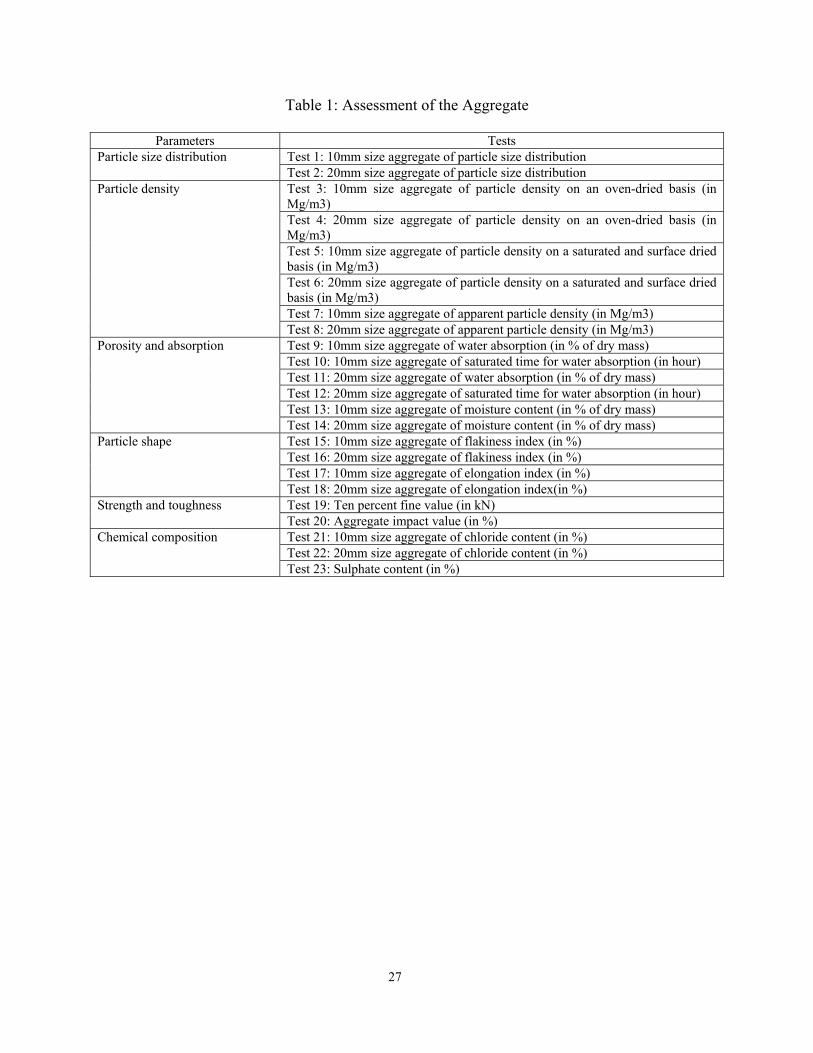
Aggregate quality is assessed by using twenty three standard tests which are categorized into six

parameters in this paper (Table 1): i) particle size distribution; ii) particle density; iii) porosity

and absorption; iv) particle shape; v) strength and toughness; and vi) chemical composition.

<Table 1>

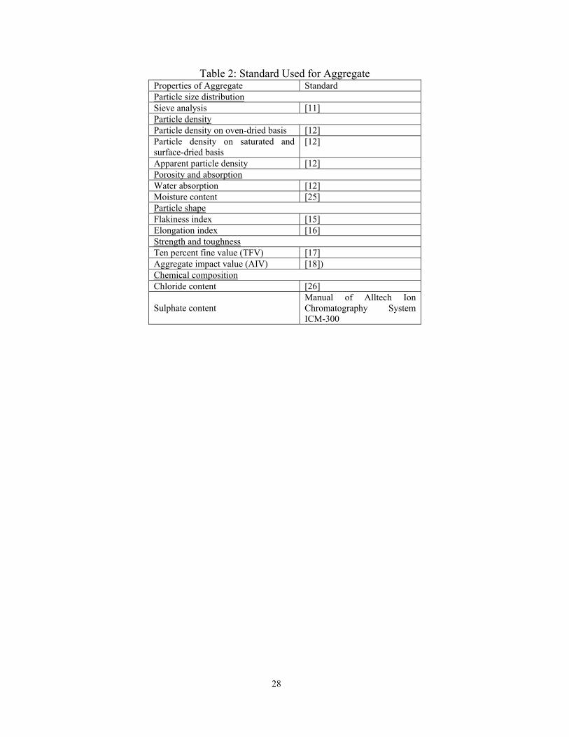
The standard methods used for testing these aggregate properties are summarized in Table 2.

<Table 2>

3 An Interpolation Process Using Vandermonde Matrix

Interpolation using polynomial fitting is a technique which uses polynomials of order up to 20 to

fit a given set of data. This technique is well known because it is much better than the linear

regression method of simply assigning the “line of best fit” to the data. Given a set of data in the

form of x(1), x(2),…, x(N), with values of y(1), y(2),…, y(N), where N is the data length. The

coefficients c1, c2, …, cN of the interpolating polynomial which can be used to "best fit" the data

relate the input x to the output y via the Vandermonde matrix of the form [5]:

⎥⎥⎥⎥

⎦

⎤

⎢⎢⎢⎢

⎣

⎡

=

⎥⎥⎥⎥

⎦

⎤

⎢⎢⎢⎢

⎣

⎡

⎥⎥⎥⎥⎥

⎦

⎤

⎢⎢⎢⎢⎢

⎣

⎡

−

−

−

NNNNNN

N

N

y

yy

c

cc

xxx

xxxxxx

......

...1...............

...1

...11

0

1

0

12

11

211

10

200

,

(1)

5

where the c matrix consists of coefficients of the polynomial. It should be stressed that the c

matrix does not always exist; prompting that extra care must be taken when using the technique

to interpolate different data sets.

Having obtained the c matrix, the interpolating polynomial is thus given by:

yinterpolate = cNxN + cN–1xN–1 + … +c1x + c0, (2)

which can be used to mathematically model the given data. It should also be noted that yinterpolate

generally resembles the shape of the fitted data. However, sometimes, it is difficult to find all

coefficients for a particular data set. Thus, if the method is applicable to a set of data, then the

process of studying and simulation the data becomes much easier and less time consuming as

yinterpolate can now be validly used. However, no numerical methods can completely simulate a

given set of data, thus, there exists some marginal errors in curve fitting which generally do not

significantly alter the results obtained by analysing yinterpolate. Even though interpolation and

spectral techniques have been widely used in the field of signal and image processing [5], they

have not been widely used in the field of construction material and management to process data

and to study their correlation.

Out of the twenty-three tests, the first two tests do not have numerical results, leaving tests three

to twenty three applicable for interpolation. Every test from three to twenty three is then used as

an input with the other tests as outputs to obtain their mathematical relationships with the input

test. For example, the first patch of interpolation uses test three as the input, thus tests four to

twenty three are used as the outputs. As a result, the relationships between test pairs four and

three, five and three, six and three and so on until the last test pairs of twenty three and three are

6

obtained. In the second patch of interpolation, test four is used as the input and tests five, six,

seven until twenty three as the outputs. The interpolation process continues until test twenty two

is taken as the input and test twenty three as the output, in this case, there is only one pair of

input and output in the interpolation patch. At the end of the whole interpolation process, by

using one order, there are two hundred and ten equations describing the mathematical

relationships among all the tests, i.e. every test is interpolated with every other test, and therefore

it is not difficult to estimate the results of a particular test using one of the many equations

obtained from the interpolation process. Ten different order polynomials are used to interpolate

the data, yielding two thousand and one hundred equations relating the results of all tests. The

challenge is to choose the best polynomials with the lowest fitting errors. Fitting errors are

estimated by taking the difference of the interpolation polynomial and the real data. Because

there are ten different polynomial orders, there exist ten different mathematical equations which

can be used to estimate the results of test four. The same process is carried out for all tests and in

all orders. It is clear that the more polynomials the interpolation process uses, the easier it is to

simplify aggregate testing procedures as there is more than one equation relating results of

particular input to a particular output available for selection. The main difference of this paper

and other papers is to use spectral methods such as power spectra and bispectrum to study the

fitting errors instead of estimating the error’s mean, thus revealing error uniformness and

distribution. To choose satisfactory polynomials, the error upper limit is chosen to be 15% in this

paper. It should be noted that interpolation equations possessing errors larger than the upper limit

are considered to be invalid and hence cannot be used to estimate the results of the other tests.

7

The interpolating polynomials can be generated by using the MATLAB package via the

command polyfit. The order of the polynomials is considered to be an important parameter.

For this particular set of data, polynomial orders of one to ten are used to thoroughly study the

effectiveness of the method. It should also be noted that the higher the order of the polynomial,

the better the fit to the data. However, for data consisting of many abrupt changes, high-order

polynomials cannot satisfactorily interpolate the data as will be shown later.

4 Spectral Methods

4.1 The Fourier Transform

The Fourier transform is a useful and powerful tool employed to study "frequency" components

of signals and discrete data which are usually recorded in the time domain. After transforming

the data into the frequency domain using the Fourier transform, the signal energy distribution at

different frequencies is revealed. Effectively, the Fourier transform can be considered as a prism

where white light can be split into its individual spectra. For the case of the Fourier transform,

the signal energy is split over the signal's spectrum which consists of a number of frequencies at

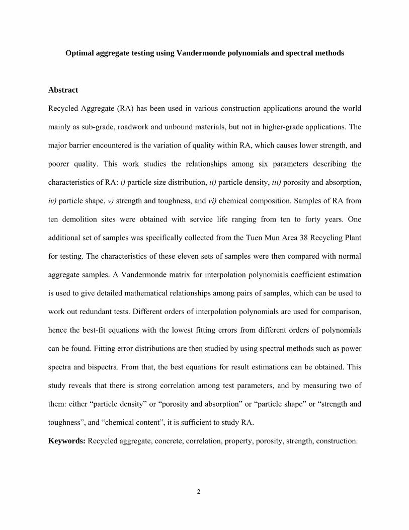
which harmonics and sub-harmonies are displayed. Mathematically, the Fourier transform X( f )

as a function of the frequency f is given as [6]:

dtetxfX ftj π2)()( −

+∞

∞−∫= ,

(3)

where j2 = −1 is a complex constant, π ≈ 3.1415 and x(t) the input signal or data. The input data

or signal is usually a 1-D array or 2-D matrix.

8

To recover a time signal from its Fourier transform, the inverse Fourier transform is employed,

which is mathematically given as:

dfefXtx ftj π2)()( +

+∞

∞−∫= .

(4)

It should be noted that the Fourier transform is a complex number which is uniquely described

by its magnitude and phase. Thus, it is clear that there are two ways of representing data: in the

time domain and in the frequency domain using the Fourier transform. The transformation from

time domain to frequency domain is achieved by using the operator e jωt, which can be given in

Eq. (5) as:

e jωt = cos(ωt) + jsin(ωt). (5)

Frequency is normally defined as the number of repetitions over time and the concept of

"frequency domain" is believed to be new in the field of construction material and management.

Frequency is inversely proportional to time, which means the larger the time, the smaller the

frequency and vice versa. Using the concept of frequency and time it can be said that data which

have a long time span have densely-concentrated spectra over a short frequency range and vice

versa. The magnitude of the frequency components which are displayed over a frequency range

or spectrum is defined as proportional to the signal energy. Signals which are continuous and

periodic in time have densely concentrated energy spectra. For ease of understanding, the Fourier

transform can be viewed as a mapping the energy distribution in the signal in the frequency

domain at which harmonic peaks or dominant peaks represent the peak energy concentration in

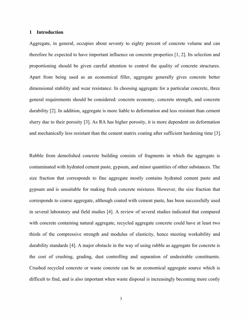
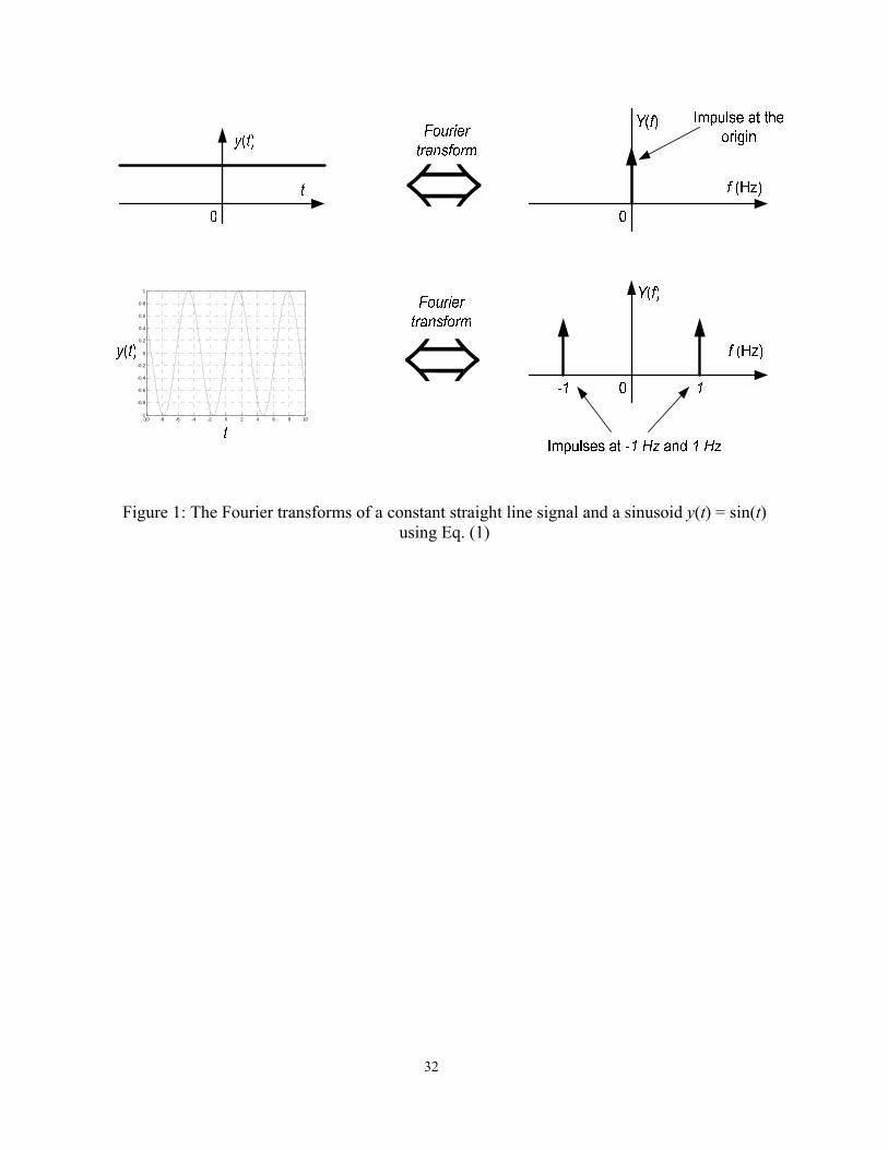
the waveform. For example, the Fourier transform of a constant signal which is continuous from

9

−∞ to +∞ is an impulse whose energy concentration is theoretically perfect. A common and

popular sinusoidal signal of frequency f0 = 1 Hz has two impulses located at ±1 Hz as shown in

Figure 1.

<Figure 1>

4.2 The Power Spectrum

The interpolation method is used to estimate the results of output tests from input tests. From that,

it is possible to determine redundancy among the tests, in turn, significantly lowers the number

of tests. To further study the correlation among the tests, spectral methods using the power

spectrum and bispectrum are employed. The power spectrum P( f ) of a data set x(t) is given in

Eq. (6) as:

P( f ) = | X( f ) |2, (6)

where X( f ) is the Fourier transform of the data or input signal. It is evident that the power

spectrum is proportional to the square magnitude of the input signal’s Fourier transform as

expected because the signal energy is directly related to its squared magnitude. It is important to

stress that energy plays an important role in determining data characteristics, i.e. periodic,

aperiodic or chaotic, detecting transitions from one state to another, i.e. from periodicity to chaos

or periodicity to transient, and working out the energy weighting at different frequencies [6]

which can be achieved by estimating the power spectrum of the input data. In the case of

studying sample results of tests in construction material and management, the power spectrum is

particularly useful as it can reveal the energy distribution of samples in each test. From that, the

significance of each test can be assessed. In addition, the power spectrum can be used to classify

different types of data including periodic, chaotic, transient and noise by interpreting its shapes

10

and frequency range [7]. Recently, the power spectral method has been successfully used to

identify dominant criteria [8] in environmental surveys by studying their energy distribution.

Moreover, as data processing and analyses are increasingly important, this further strengthens the

idea of using spectral methods in the field of construction material and management. The only

drawback of the power spectrum is that its phase information is suppressed which means that

two different data sets could have identical power spectra. To overcome this problem and to

further study the correlation among the tests and samples, the bispectral method is employed.

4.3 The Bispectrum

To further study the data, a bispectral method is introduced which shows the correlation among

the tests at various "frequencies". The bispectrum B( f1, f2 ) has been widely employed in the

field of high-order statistics to study data correlation in 3-D and is given by [9]:

B( f1, f2 ) = X( f1 )X( f2)X*( f1 + f2), (7)

where the symbol " * " means complex conjugate.

It is clear that the bispectrum is strongly dependent on the Fourier transform of the input signal.

From Eq. (7), the term X*( f1 + f2) represents the correlation among various frequency terms in

the ( f1 + f2) plane. To estimate the bispectrum, the mean value of the data is removed to

eliminate sudden spikes and pulses which could lead to misleading interpretation. In MATLAB,

this can be done by using a detrend(⋅) function. After that, the data are windowed using a

Hanning window via the command hanning(⋅) provided in MATLAB. In addition, the data

are also normalised by dividing each column by its largest item so that abrupt changes are

nullified. The Fourier transforms of the detrended data are then calculated, in this case, there are

11

twenty one out of twenty three tests having numerical results, yielding twenty one Fourier

transforms. In this paper, the bispectrum of an error matrix of 210×10 is calculated to show

correlation among the fitting errors and also error uniformness.

Unlike the power spectrum which suppresses the phase information in the data, the bispectrum

uniquely gives the phase information, i.e. the correlation among a number of frequencies, which

enable detailed studied on correlation among the tests. It should also be stressed that because the

bispectrum gives both the magnitude and phase information, it is considered to be unique, i.e.

different data possess unique and different bispectra. However, because the phase information is

usually difficult to interpret, the magnitude bispectrum is usually employed as the main tool for

data analyses.

5 The Study

Ten series of RA samples (Samples one to ten) were obtained from ten demolition sites with

service life ranging from ten to forty years. Sample eleven was specifically collected from the

Tuen Mun Area 38 Recycling Plant. Samples one to eleven are then compared with normal

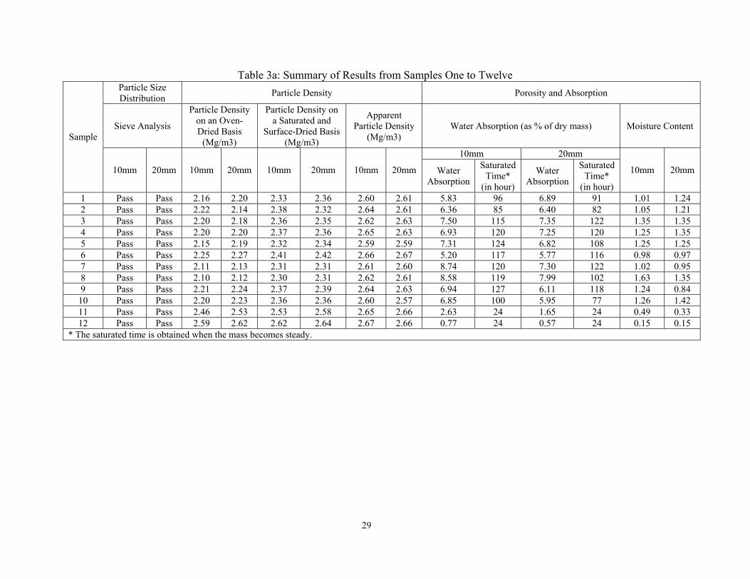
aggregate which is Sample twelve. The results of twenty three tests for Samples one to twelve

are summarized in Table 3.

<Table 3>

5.1 Particle Size Distribution

Since the strength of fully compacted concrete with a given water/cement ratio is independent of

the particle size distribution (sieve analysis of the aggregate), sieve analysis is important only if

12

it affects fresh concrete workability [10]. Samples one to twelve have met the particle size

distribution criterion of being ten mm and twelve mm single-size aggregate as stated in BS 882

[11] (see Table 3).

5.2 Particle Density

The particle density of aggregate is the ratio of the mass of a given volume of material to the

mass of the same volume of water [12]. Aggregate particle density usually is an essential

property for concrete mix design and also for calculating the volume of concrete produced from

a certain mass of materials [13]. As the density of cement mortar [around 1.0-1.6 Mg/m3] is less

than that of stone particles of about 2.60 Mg/m3 [14], the smaller the particle density, the higher

the cement mortar content adhering to the RA. The average results of the three different tests

based on oven-dried basis, saturated and surface-dried basis, and apparent particle density, were

measured and are presented in Table 3.

From Table 3, Samples seven and eight have the lowest values of particle density, inferring the

highest amount of cement mortar adhering to RA, while Sample twelve (normal aggregate) has

the highest particle density. Furthermore, particle densities of twenty mm aggregate are larger

than those of ten mm aggregate, inferring a higher amount of cement mortar attached to the ten

mm aggregate. This also implies that the larger the aggregate size, the smaller the amount of

cement mortar attached to its surface, yielding better aggregate quality.

Polynomial fitting of tests (outputs) based on the results of a particular test (input) can be

achieved by using an appropriate polynomial order. Generally, the higher the polynomial order,

13

the better the fitting. However, it is not always the case if there are abrupt changes in the outputs

because a very high-order polynomial is required, which is not practical if the order is larger than

the upper limit of twenty given in MATLAB. Thus, care must be taken to choose the appropriate

order for the interpolation polynomial, otherwise large errors can be generated. The fitting errors

of all orders are given to assess the effectiveness and validity of each order (see Appendix II).

Equations (8) to (217) mathematically describe the relationship among the tests and are given in

Appendix I. Equations (8) to (112) give the relationships of tests four to twenty three which are

considered as the outputs using the best-fit polynomials. Simulation results show that the errors

for tests three to twenty are mostly acceptable with the maximum errors lower than the chosen

error limit of 15%.

5.3 Porosity and Absorption

The overall porosity or absorption of aggregate either depends on a consistent degree of particle

porosity or represents an average value for a mixture of variously high and low absorption

materials [13]. In this study, both the rate of water absorption and moisture content are used to

assess the level of porosity and absorption of the samples.

The water absorption and moisture content of recycled aggregate (Samples one to twelve) are

generally higher than that of normal aggregate (Sample twelve) (see Table 3). Ten mm size

aggregate of Sample seven exhibits the highest water absorption rate and moisture content of

about 9.06 and 1.70 respectively, and twenty mm aggregate from Sample twelve has the lowest

water absorption rate and moisture content of about 0.53 and 0.15 respectively. One of the most

14

obvious attributes between RA and normal aggregate is the higher water absorption rate and

moisture content, which are affected by the amount of cement paste sticking on the aggregate

surface. Cement mortar describes the soundness of aggregate since its porosity is higher than that

of aggregate, i.e. RA with higher absorption rate tends to be worsened in strength and resistance

under freezing and thawing conditions [18-20] than aggregate with a lower absorption rate. In

most samples, the water absorption rate of twenty mm aggregate is less than that of ten mm

aggregate, inferring that larger size aggregate may have less cement mortar adhered to its surface,

leading to a lower water absorption rate as explained in the last section.

Using a standard testing method [12] of waiting for twenty four hours before measuring water

absorption is not appropriate for recycled aggregate due to the high amount of loosely-bonded

cement paste on particles resulted from the crushing process. Experiments showed that the

required time to fully saturate RA depends on its quality which can be determined by the amount

of cement paste adhering on its surface. In most cases, the required time is more than twenty four

hours. From experiment, it is believed that full saturation can take up to forty-eight hours; some

may take seventy-two hours or even one hundred and twenty hours. Thus, a fixed duration of

twenty-four hours set by BS 812: Part 2 [12] may not be sufficient for RA. Relationships of tests

ten to twenty three as the outputs based on tests nine to fourteen as the inputs are described by

Equations (113) to (181) using the best-fit polynomials.

5.4 Particle Shape

The characteristics and variations of the shape of aggregate particles can affect concrete strength

and workability [13]. The shape of aggregate particles is best described by using two principal

15

parameters: ‘sphericity’ and ‘roundness’. Aggregate particles are classified as flaky when they

have a thickness (smaller dimension) of less than 0.6 of their mean sieve size. For example, a

mean sieve size of 7.5mm is the mean of two successive sieves at five mm and ten mm [15].

Aggregate particles are classified as elongated when they have a length (greatest dimension) of

more than 1.8 of their mean sieve size [16].

BS 882 [11] now provides limits for flakiness (particle thickness relative to other dimensions).

Such aggregate particles could lead to either water gain under the aggregate, causing planes of

weakness, or higher water demand and lower strength in concrete. BS 882 [11] limits the

flakiness index determined in accordance with BS 812: Part 105:1 [15] to about fifty percent for

uncrushed gravel and forty percent for crushed rock or crushed gravel, with a warning that lower

values may have to be specified for special circumstances such as pavement wearing surfaces.

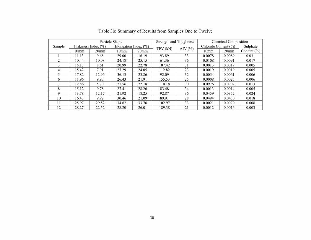
All the twelve samples in this study have a flakiness index lower than forty percent.

Mathematical relationships of tests sixteen to twenty three as the outputs based on tests fifteen to

eighteen as the inputs are given in Equations (182) to (207) by using the best-fit polynomials.

5.5 Strength and Toughness

It is important that aggregate used for concrete be ‘strong’ in a general sense [14]. In most cases,

inherent aggregate strength is dependent upon aggregate ‘toughness’, a property broadly

analogous to ‘impact strength’. In this study, Ten percent Fine Values (TFV) and Aggregate

Impact Values (AIV) are used to determine the strength and toughness of the twelve samples.

16

The TFV measures the resistance of aggregate to crushing which is applicable to both weak and

strong aggregates [17], the larger the TFV value, the more resistant the aggregate to crushing

[13]. The AIV relatively measures the resistance of aggregate to sudden shock or impact, which

in some aggregate is different from its resistance to a slowly applied compressive load [18]. The

smaller the AIV value, the tougher the aggregate or more impact resistant than higher strength

concrete aggregate [13]. Out of the twelve samples, Sample twelve (ordinary aggregate) has the

highest value of TFV and the lowest value of AIV at 189 kN and 21% respectively; while

Sample two achieves the lowest value of TFV and the highest value of AIV at 61 kN and 36%

respectively (see Table 3). The obvious reason is that the cement paste attached to the RA

directly affects its strength.

BS 882 [11] provides limits for TFV and AIV, minimum of 150 kN and 45% respectively

according to the type of concrete in which the aggregate is used. According to the British

Standard, Samples six and twelve can be used for structural elements, Samples four and seven

for pavement work and other samples confined to non-structural elements. The mathematical

relationships of tests twenty to twenty three as the outputs based on tests nineteen and twenty as

the inputs are given in Equations (208) to (214) by using the best-fit polynomials.

5.6 Chemical Composition

Chloride and sulphate contents of RA are critical. Chloride contamination of recycled aggregate

mainly derived from marine structures or similarly exposed structural element is of concern

which can lead to corrosion of steel reinforcement. However, for most RA (Samples one to six

and eight to twelve), the chloride ion contents are low and within the limit of standards (under

17

0.05%). Nevertheless, Sample seven falls beyond the limit with chloride contents of about

0.0976% and 0.0902% for ten mm and twenty mm aggregates respectively (see Table 3). From

further investigation of the RA of Sample seven, some shell (from fine marine aggregate)

contents were found. The major reason may be the use of marine water or stream water for

concrete mixing during periods of shortage of fresh water supply in the 1960s, which has been

banned since 1970s. This could have increased the chloride composition in the sample.

In general, RA has higher sulphate content than natural aggregate. The occurrence of sulphate-

based products such as plaster as contaminants in demolition waste is common. Consideration

must be given to the use of sulphate resisting cement in situation where plaster contamination is

suspected [19]. However, gypsum plaster is rarely used in Hong Kong where lime plaster is more

common. In fact, the highest recorded sulphate content is about 0.0308% for Sample one, which

is still within the standard of 1% (see Table 3). Therefore, contamination of sulphate content is

not a major problem for RA in Hong Kong. The mathematical relationships of tests twenty two

and twenty three as the outputs with tests twenty one and twenty two as the inputs are given in

Equations (215) to (217) by using the best-fit polynomials.

Using the results obtained in Sections 5.1 to 5.6, the best-fit polynomials are shown in Equations

(8) to (217). From the results obtained in this paper, the tests can be divided into two major

groups: group one consists of tests three to twenty, and group two consists of tests twenty one to

twenty three. It is clear that the tests in group one are strongly correlated which are given in

Equations (8) to (214). This means that the results of any test in this group can be successfully

estimated by using the results of another test from the same group. The error percentage of the

18

first test group is satisfactory. However, there are a small number of tests possessing errors of

more than 15%, which do not affect the findings in this paper since there is more than one

mathematical expression describing them.

It should also be noted that there are some satisfactory relationships among the three tests in the

second test group (tests twenty one to twenty three). However, most equations in this group

possess high error percentage which suggests that they are poorly correlated. It can be suggested

not to use Equations (215) to (217) to predict the results of tests in the first test group to estimate

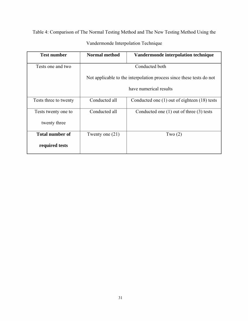
the results of the second test group. As a result, two tests out of tests three to twenty three are

required instead of twenty one tests being routinely conducted in the industry. In addition to tests

one and two, there are four tests which are required to be conducted. It should also be noted that

out of tests three to twenty, the results of only one of these tests is required which provides

flexibility in conducting the tests depending on the conditions and available equipment. As

construction sites in Hong Kong are limited in size, eliminating redundant tests significantly

lowers cost and shortens aggregate testing time, yielding more efficient space usage on site and

many other benefits for the construction industry. Table 4 summarises the findings of the paper.

<Table 4>

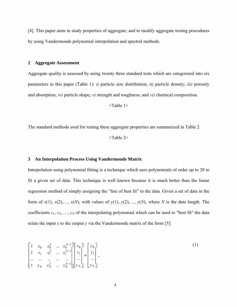
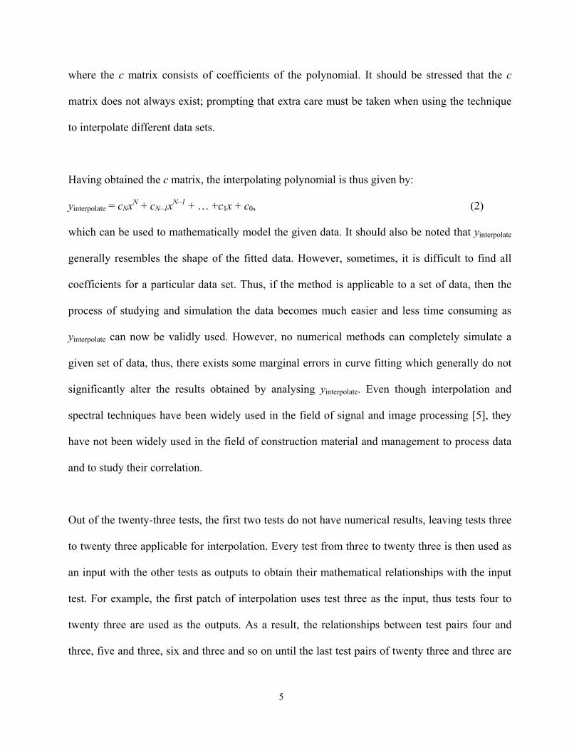
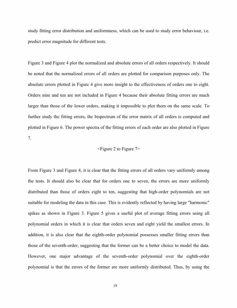
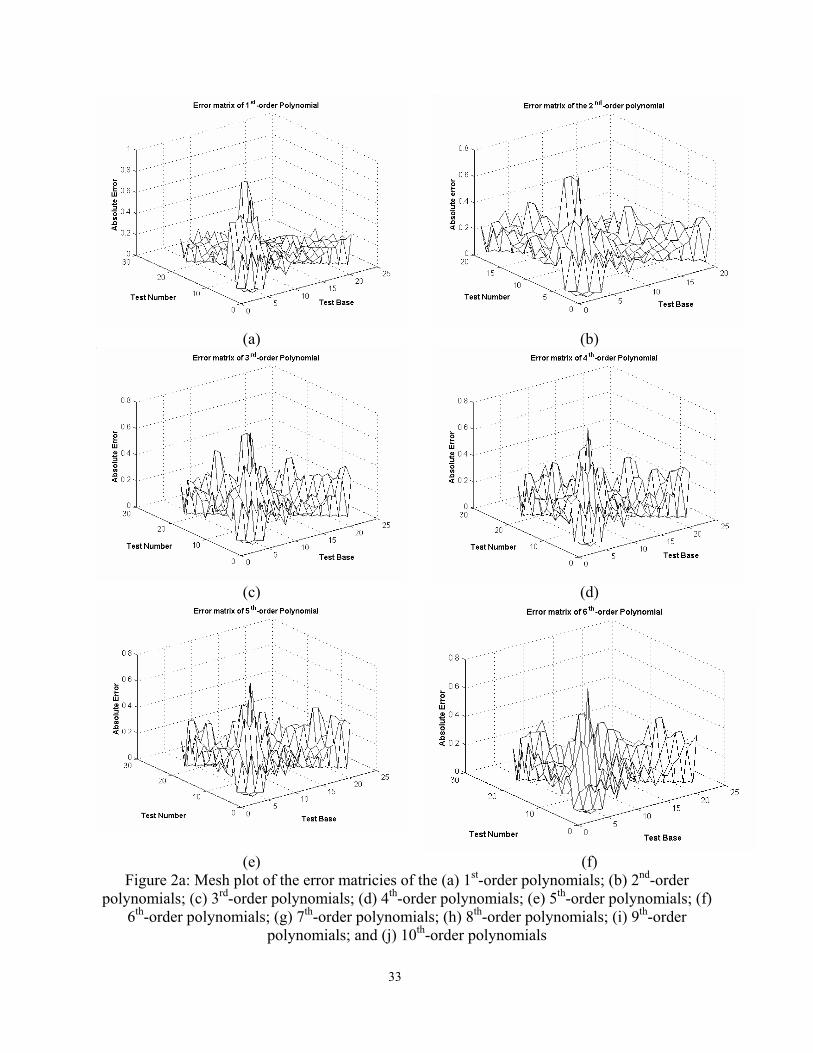
To assess the effectiveness of the interpolation process using different orders, fitting errors of

interpolation polynomials of orders one to ten are estimated and given in Figure 2. Fitting errors

are the difference between the real data and values of the corresponding polynomials. It is clear

that the smaller the fitting error, the better the polynomial fitting. The maximum allowable fitting

error is chosen to be 15% in this paper. In addition, by using spectral methods, it is possible to

19

study fitting error distribution and uniformness, which can be used to study error behaviour, i.e.

predict error magnitude for different tests.

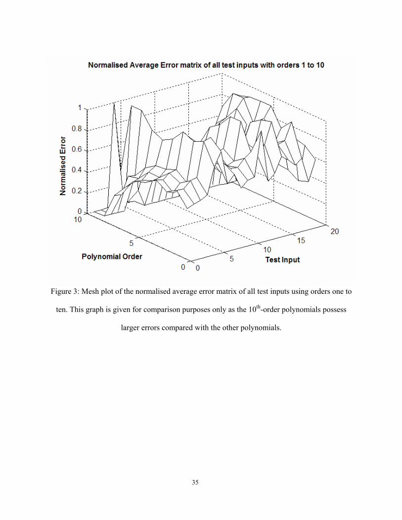
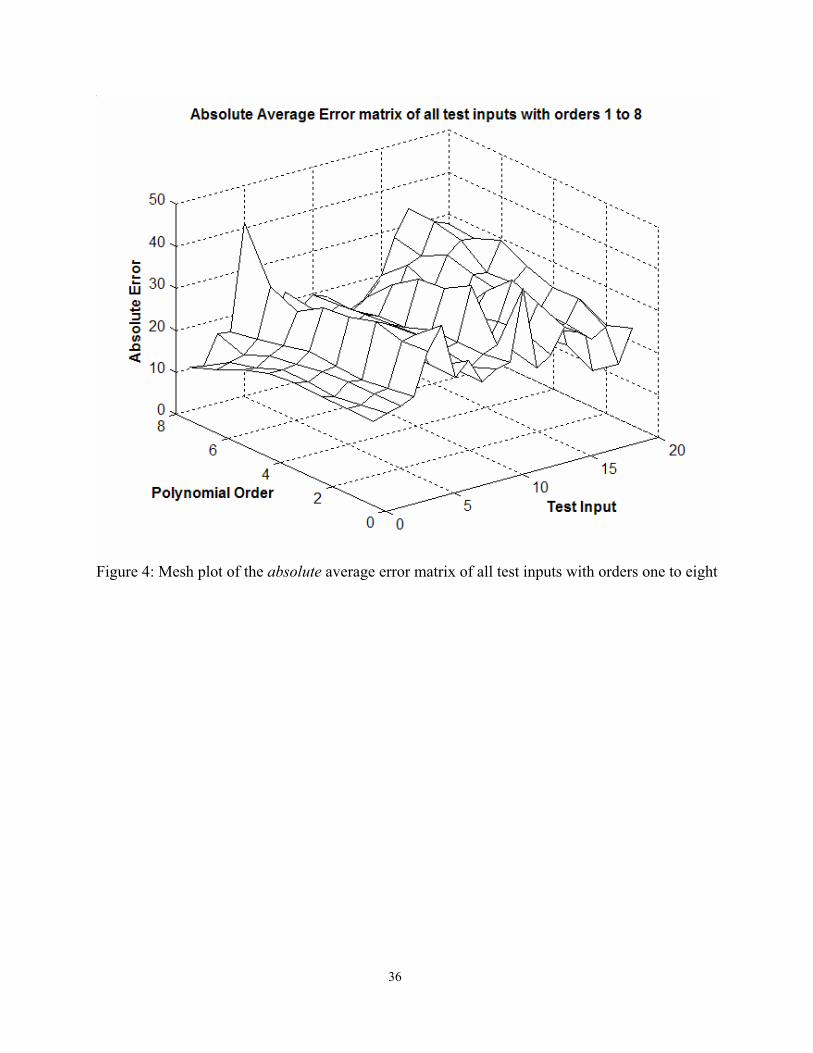
Figure 3 and Figure 4 plot the normalized and absolute errors of all orders respectively. It should

be noted that the normalized errors of all orders are plotted for comparison purposes only. The

absolute errors plotted in Figure 4 give more insight to the effectiveness of orders one to eight.

Orders nine and ten are not included in Figure 4 because their absolute fitting errors are much

larger than those of the lower orders, making it impossible to plot them on the same scale. To

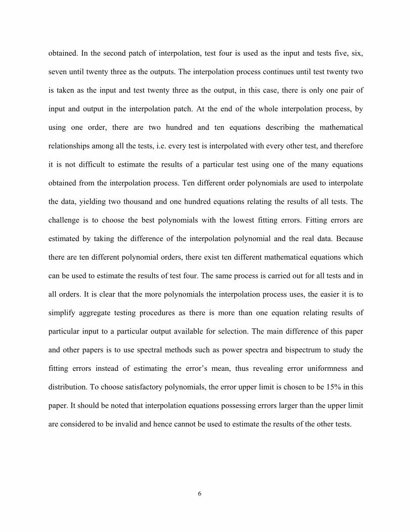
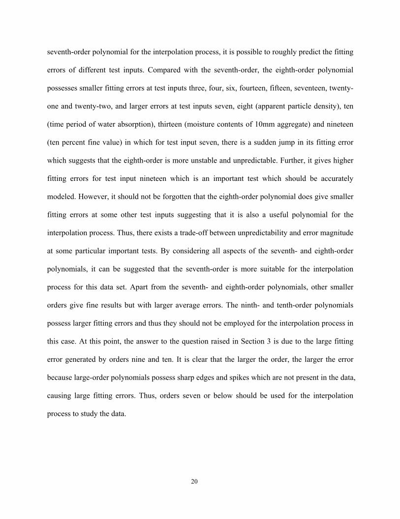
further study the fitting errors, the bispectrum of the error matrix of all orders is computed and

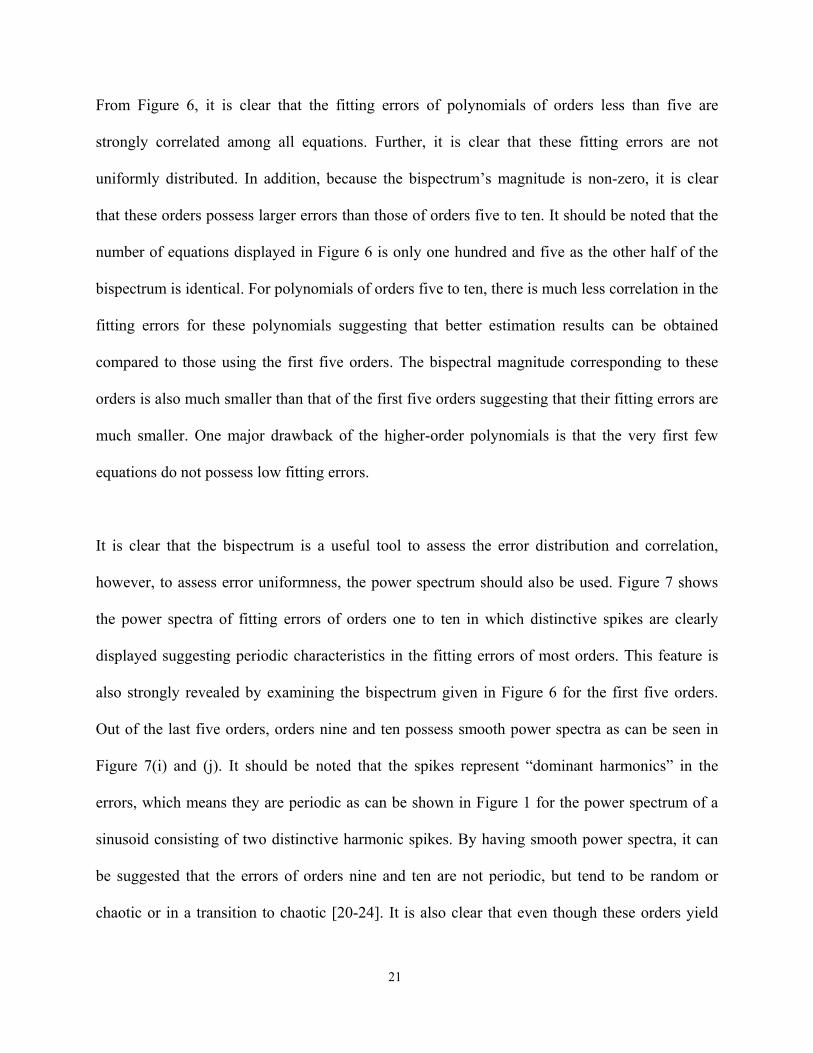
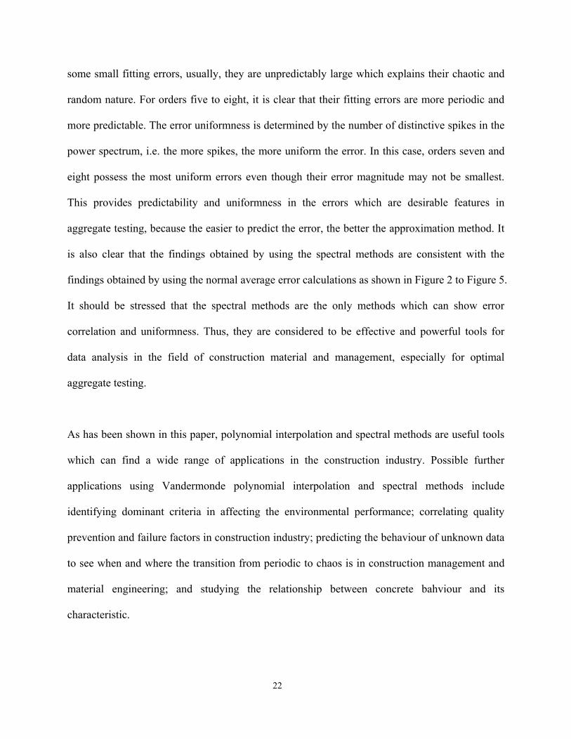
plotted in Figure 6. The power spectra of the fitting errors of each order are also plotted in Figure

7.

<Figure 2 to Figure 7>

From Figure 3 and Figure 4, it is clear that the fitting errors of all orders vary uniformly among

the tests. It should also be clear that for orders one to seven, the errors are more uniformly

distributed than those of orders eight to ten, suggesting that high-order polynomials are not

suitable for modeling the data in this case. This is evidently reflected by having large "harmonic"

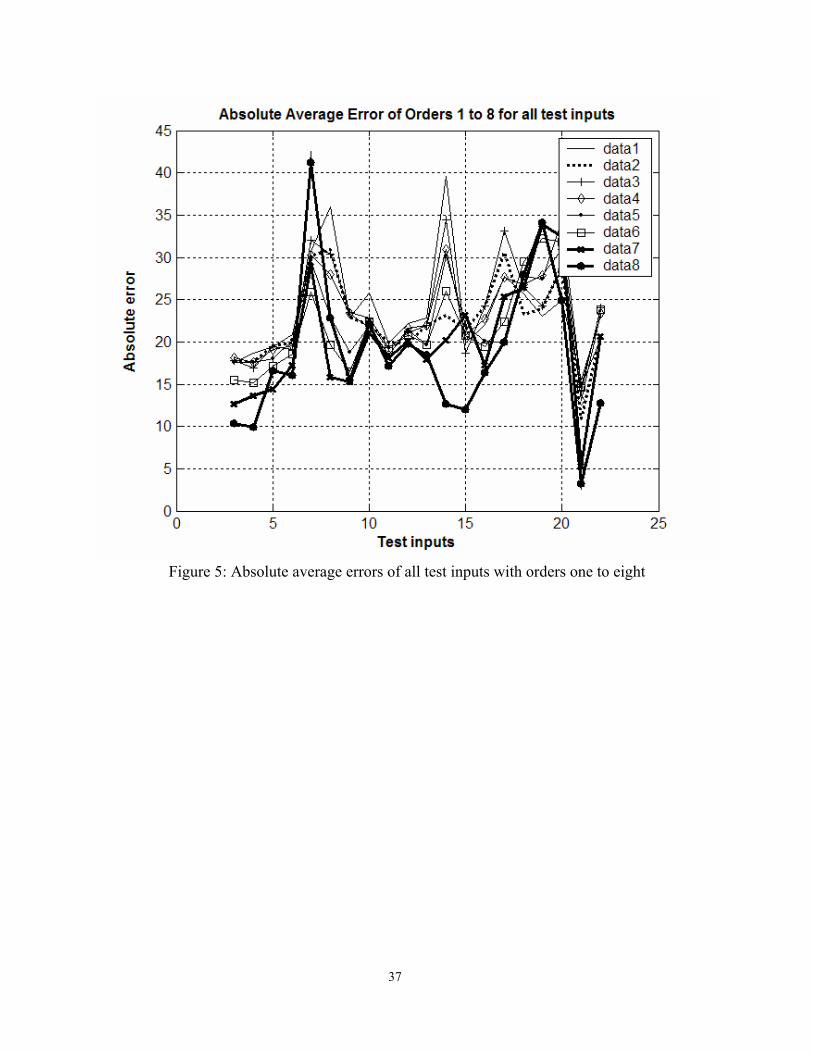
spikes as shown in Figure 3. Figure 5 gives a useful plot of average fitting errors using all

polynomial orders in which it is clear that orders seven and eight yield the smallest errors. In

addition, it is also clear that the eighth-order polynomial possesses smaller fitting errors than

those of the seventh-order, suggesting that the former can be a better choice to model the data.

However, one major advantage of the seventh-order polynomial over the eighth-order

polynomial is that the errors of the former are more uniformly distributed. Thus, by using the

20

seventh-order polynomial for the interpolation process, it is possible to roughly predict the fitting

errors of different test inputs. Compared with the seventh-order, the eighth-order polynomial

possesses smaller fitting errors at test inputs three, four, six, fourteen, fifteen, seventeen, twenty-

one and twenty-two, and larger errors at test inputs seven, eight (apparent particle density), ten

(time period of water absorption), thirteen (moisture contents of 10mm aggregate) and nineteen

(ten percent fine value) in which for test input seven, there is a sudden jump in its fitting error

which suggests that the eighth-order is more unstable and unpredictable. Further, it gives higher

fitting errors for test input nineteen which is an important test which should be accurately

modeled. However, it should not be forgotten that the eighth-order polynomial does give smaller

fitting errors at some other test inputs suggesting that it is also a useful polynomial for the

interpolation process. Thus, there exists a trade-off between unpredictability and error magnitude

at some particular important tests. By considering all aspects of the seventh- and eighth-order

polynomials, it can be suggested that the seventh-order is more suitable for the interpolation

process for this data set. Apart from the seventh- and eighth-order polynomials, other smaller

orders give fine results but with larger average errors. The ninth- and tenth-order polynomials

possess larger fitting errors and thus they should not be employed for the interpolation process in

this case. At this point, the answer to the question raised in Section 3 is due to the large fitting

error generated by orders nine and ten. It is clear that the larger the order, the larger the error

because large-order polynomials possess sharp edges and spikes which are not present in the data,

causing large fitting errors. Thus, orders seven or below should be used for the interpolation

process to study the data.

21

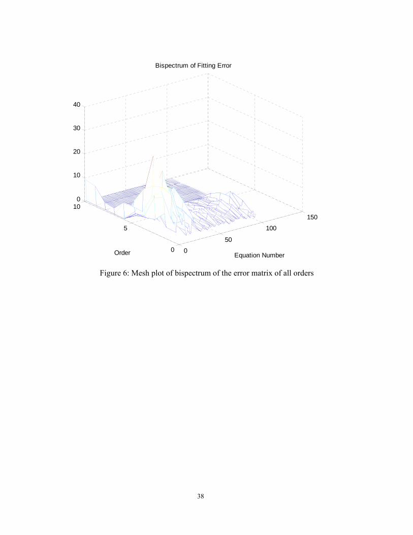
From Figure 6, it is clear that the fitting errors of polynomials of orders less than five are

strongly correlated among all equations. Further, it is clear that these fitting errors are not

uniformly distributed. In addition, because the bispectrum’s magnitude is non-zero, it is clear

that these orders possess larger errors than those of orders five to ten. It should be noted that the

number of equations displayed in Figure 6 is only one hundred and five as the other half of the

bispectrum is identical. For polynomials of orders five to ten, there is much less correlation in the

fitting errors for these polynomials suggesting that better estimation results can be obtained

compared to those using the first five orders. The bispectral magnitude corresponding to these

orders is also much smaller than that of the first five orders suggesting that their fitting errors are

much smaller. One major drawback of the higher-order polynomials is that the very first few

equations do not possess low fitting errors.

It is clear that the bispectrum is a useful tool to assess the error distribution and correlation,

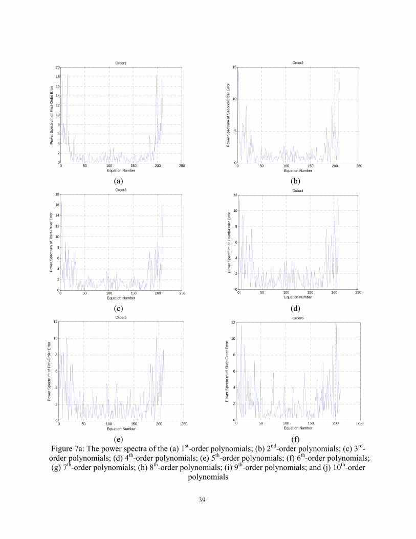
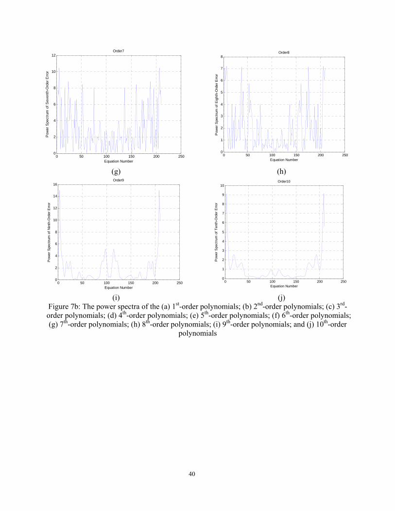
however, to assess error uniformness, the power spectrum should also be used. Figure 7 shows

the power spectra of fitting errors of orders one to ten in which distinctive spikes are clearly

displayed suggesting periodic characteristics in the fitting errors of most orders. This feature is

also strongly revealed by examining the bispectrum given in Figure 6 for the first five orders.

Out of the last five orders, orders nine and ten possess smooth power spectra as can be seen in

Figure 7(i) and (j). It should be noted that the spikes represent “dominant harmonics” in the

errors, which means they are periodic as can be shown in Figure 1 for the power spectrum of a

sinusoid consisting of two distinctive harmonic spikes. By having smooth power spectra, it can

be suggested that the errors of orders nine and ten are not periodic, but tend to be random or

chaotic or in a transition to chaotic [20-24]. It is also clear that even though these orders yield

22

some small fitting errors, usually, they are unpredictably large which explains their chaotic and

random nature. For orders five to eight, it is clear that their fitting errors are more periodic and

more predictable. The error uniformness is determined by the number of distinctive spikes in the

power spectrum, i.e. the more spikes, the more uniform the error. In this case, orders seven and

eight possess the most uniform errors even though their error magnitude may not be smallest.

This provides predictability and uniformness in the errors which are desirable features in

aggregate testing, because the easier to predict the error, the better the approximation method. It

is also clear that the findings obtained by using the spectral methods are consistent with the

findings obtained by using the normal average error calculations as shown in Figure 2 to Figure 5.

It should be stressed that the spectral methods are the only methods which can show error

correlation and uniformness. Thus, they are considered to be effective and powerful tools for

data analysis in the field of construction material and management, especially for optimal

aggregate testing.

As has been shown in this paper, polynomial interpolation and spectral methods are useful tools

which can find a wide range of applications in the construction industry. Possible further

applications using Vandermonde polynomial interpolation and spectral methods include

identifying dominant criteria in affecting the environmental performance; correlating quality

prevention and failure factors in construction industry; predicting the behaviour of unknown data

to see when and where the transition from periodic to chaos is in construction management and

material engineering; and studying the relationship between concrete bahviour and its

characteristic.

23

6 Conclusions

To have wide adoption of RA, it is essential to carefully assess its properties including particle

density, porosity and absorption, particle shape, strength and toughness, and chemical

composition. Sieve analysis should also be done to make good concrete proportioning. It has

been found that all six parameters have direct relationship with the cement mortar adhering on

the surface of aggregate leading to lower particle density, higher water absorption and lower ten

percent fine value. The RA from Sample seven exhibits the lowest quality because marine or

stream water has been used in concrete mixing, which, however, is still adoptable for non-

structural construction applications. Further, it has been found that there is strong correlation

among some of the parameters which can be used to simplify aggregate testing processes. For

example, by measuring one of “particle density”, “porosity and absorption”, “particle shape” and

“strength and toughness” and “chemical content”, it is sufficient to assess the characteristic and

properties of RA. A new technique of using interpolation polynomials of orders one to ten has

been employed in this paper. New spectral methods using the power spectrum and bispectrum

have been introduced in this paper to study error correlation and uniformness. Fitting errors of

interpolation polynomials have been estimated in which it was shown that polynomials of orders

one to eight yield satisfactory results by providing periodic and predictable fitting errors of small

magnitude. Orders nine and ten have been shown to possess random or chaotic fitting errors

suggesting that they are not suitable for modeling the collected data presented in this paper. Out

of the ten orders, order seven is the optimum order for use with the interpolation technique to

process the data. This paper has shown that interpolation techniques can be successfully used to

process data in the field of construction material and management.

24

7 References

1. S. Mindess F. Young D. Darwin. Concrete. ed. Upper Saddle River, N.P.H.2003.

2. G.E. Troxell H.E. Davis. Composition and properties of concrete. New York: McGraw-Hill,

1968.

3. J.C. Maso. Influence of the interfacial transition zone on composite mechanical properties.

Interfacial transition zone in concrete: state of the art report, 1996, London: E & FN Spon

103-116.

4. P.K. Mehta J.M. Monteiro. Concrete: structure, properties, and materials. ed. Englewood

Cliffs, N.J.P.H.1993.

5. W.H. Press S.A. Teukolsky W.T. Vetterling B.P. Flannery. Numerical Recipes in C. New

York: Cambridge University Press, 1994.

6. B.P. Lathi. Modern Digital and Analog Communication Systems. NewYork: Oxford

University Press, 1998.

7. K.N. Le K.P. Dabke G.K. Egan. Hyperbolic wavelet power spectra of non-stationary signals.

Optical Engineering. 2003;42(10): 3017-3037.

8. W.Y.V. Tam K.N. Le. The six-sigma principle and prevention-appraisal-failure modeling for

quality improvement in construction. Building and Environment. 2006: Article in press.

9. B.P.v. Milligen C. Hidalgo E. Sanchez. Nonlinear phenomena and intermittency in plasma and

turbulence. Physical Review Letters. Jan. 1995;74(3): 395-8.

10. A.M. Neville. Properties of concrete. ed. Burnt Mill, H., Essex; New York, Longman1995.

11. BS 882. Specification for aggregates from natural sources for concrete. British Standards

Institution, London, United Kingdom, 1992.

25

12. BS 812: Part 2. Methods for determination of density. British Standards Institution, London,

United Kingdom, 1995.

13. P.C. Hewlett. Lea's chemistry of cement and concrete. London: Arnold, 1998.

14. Oklahoma State University. Recycled Aggregate. http://osu.okstate.edu/

15. BS 812: Part 105.1. Flakiness index. British Standards Institution, London, United Kingdom,

1989.

16. BS 812: Part 105.2. Elongation index of coarase aggregate. British Standards Institution,

London, United Kingdom, 1989.

17. BS 812: Part 111. Methods for determination of ten per cent fines value (TFV). British

Standards Institution, London, United Kingdom, 1990.

18. BS 812: Part 112. Methods for determination of aggregate impact value (AIV). British


19. K.S. Crentsil T. Brown. Guide for specification of recycled concrete aggregate (RCA) for

concrete production: final report.

http://www.ecorecycle.vic.gov.au/asset/1/upload/Guide_for_Specification_of_Recycled_

Concrete_Aggregates_(RCA).pdf

20. D.S. Dabby. Musical variations from a chaotic mapping. Chaos. 1996;6(2): 95-107.

21. H. Franco. Wavelet analysis of a nonlinear oscillator transient during synchronization.

International Journal of Bifurcation and Chaos. 1996;6(12B): 2557-70.

22. B.A. Jubran M.N. Hamdan N.H. Shabaneh. Wavelet and chaos analysis of flow induced

vibration of a single cylinder in cross-flow. International Journal of Engineering Science.

1998;36(7-8): 843-64.

http://osu.okstate.edu/

http://www.ecorecycle.vic.gov.au/asset/1/upload/Guide_for_Specification_of_Recycled_Concrete_Aggregates_(RCA).pdf

http://www.ecorecycle.vic.gov.au/asset/1/upload/Guide_for_Specification_of_Recycled_Concrete_Aggregates_(RCA).pdf

26

23. B.A. Jubran M.N. Hamdan N.H. Shabanneh. Wavelet and chaos analysis of irregularities of

vortex shedding. Mechanics Research Communications. 1998;25(5): 583-91.

24. W.J. Staszewski K. Worden. Wavelet analysis of time-series:Coherent structues, chaos and

noise. International Journal of Bifurcation and Chaos. 1999;9(3): 455-71.

25. BS 812: Part 109. Method for determination of moisture content. British Standards Institution,

London, United Kingdom, 1990.

26. BS 812: Part 117. Methods for determination of water-soluble chloride salts. British


27

Table 1: Assessment of the Aggregate

Parameters Tests Test 1: 10mm size aggregate of particle size distribution Particle size distribution Test 2: 20mm size aggregate of particle size distribution Test 3: 10mm size aggregate of particle density on an oven-dried basis (in Mg/m3) Test 4: 20mm size aggregate of particle density on an oven-dried basis (in Mg/m3) Test 5: 10mm size aggregate of particle density on a saturated and surface dried basis (in Mg/m3) Test 6: 20mm size aggregate of particle density on a saturated and surface dried basis (in Mg/m3) Test 7: 10mm size aggregate of apparent particle density (in Mg/m3)

Particle density

Test 8: 20mm size aggregate of apparent particle density (in Mg/m3) Test 9: 10mm size aggregate of water absorption (in % of dry mass) Test 10: 10mm size aggregate of saturated time for water absorption (in hour) Test 11: 20mm size aggregate of water absorption (in % of dry mass) Test 12: 20mm size aggregate of saturated time for water absorption (in hour) Test 13: 10mm size aggregate of moisture content (in % of dry mass)

Porosity and absorption

Test 14: 20mm size aggregate of moisture content (in % of dry mass) Test 15: 10mm size aggregate of flakiness index (in %) Test 16: 20mm size aggregate of flakiness index (in %) Test 17: 10mm size aggregate of elongation index (in %)

Particle shape

Test 18: 20mm size aggregate of elongation index(in %) Test 19: Ten percent fine value (in kN) Strength and toughness Test 20: Aggregate impact value (in %) Test 21: 10mm size aggregate of chloride content (in %) Test 22: 20mm size aggregate of chloride content (in %)

Chemical composition

Test 23: Sulphate content (in %)

28

Table 2: Standard Used for Aggregate Properties of Aggregate Standard Particle size distribution Sieve analysis [11] Particle density Particle density on oven-dried basis [12] Particle density on saturated and surface-dried basis

[12]

Apparent particle density [12] Porosity and absorption Water absorption [12] Moisture content [25] Particle shape Flakiness index [15] Elongation index [16] Strength and toughness Ten percent fine value (TFV) [17] Aggregate impact value (AIV) [18]) Chemical composition Chloride content [26]

Sulphate content Manual of Alltech Ion Chromatography System ICM-300

29

Table 3a: Summary of Results from Samples One to Twelve Particle Size Distribution Particle Density Porosity and Absorption

Sieve Analysis

Particle Density on an Oven-Dried Basis

(Mg/m3)

Particle Density on a Saturated and

Surface-Dried Basis (Mg/m3)

Apparent Particle Density

(Mg/m3) Water Absorption (as % of dry mass) Moisture Content

10mm 20mm

Sample

10mm 20mm 10mm 20mm 10mm 20mm 10mm 20mm Water Absorption

Saturated Time*

(in hour)

Water Absorption

Saturated Time*

(in hour)

10mm 20mm

1 Pass Pass 2.16 2.20 2.33 2.36 2.60 2.61 5.83 96 6.89 91 1.01 1.24 2 Pass Pass 2.22 2.14 2.38 2.32 2.64 2.61 6.36 85 6.40 82 1.05 1.21 3 Pass Pass 2.20 2.18 2.36 2.35 2.62 2.63 7.50 115 7.35 122 1.35 1.35 4 Pass Pass 2.20 2.20 2.37 2.36 2.65 2.63 6.93 120 7.25 120 1.25 1.35 5 Pass Pass 2.15 2.19 2.32 2.34 2.59 2.59 7.31 124 6.82 108 1.25 1.25 6 Pass Pass 2.25 2.27 2.41 2.42 2.66 2.67 5.20 117 5.77 116 0.98 0.97 7 Pass Pass 2.11 2.13 2.31 2.31 2.61 2.60 8.74 120 7.30 122 1.02 0.95 8 Pass Pass 2.10 2.12 2.30 2.31 2.62 2.61 8.58 119 7.99 102 1.63 1.35 9 Pass Pass 2.21 2.24 2.37 2.39 2.64 2.63 6.94 127 6.11 118 1.24 0.84

10 Pass Pass 2.20 2.23 2.36 2.36 2.60 2.57 6.85 100 5.95 77 1.26 1.42 11 Pass Pass 2.46 2.53 2.53 2.58 2.65 2.66 2.63 24 1.65 24 0.49 0.33 12 Pass Pass 2.59 2.62 2.62 2.64 2.67 2.66 0.77 24 0.57 24 0.15 0.15

* The saturated time is obtained when the mass becomes steady.

30

Table 3b: Summary of Results from Samples One to Twelve

Particle Shape Strength and Toughness Chemical Composition Flakiness Index (%) Elongation Index (%) Chloride Content (%) Sample 10mm 20mm 10mm 20mm TFV (kN) AIV (%) 10mm 20mm

Sulphate Content (%)

1 11.13 9.68 29.00 16.19 93.89 33 0.0078 0.0089 0.031 2 10.44 10.08 24.18 25.15 61.36 36 0.0108 0.0091 0.017 3 15.17 8.61 20.99 22.78 107.42 31 0.0013 0.0019 0.005 4 15.42 7.91 27.29 24.05 112.82 23 0.0019 0.0019 0.005 5 17.82 12.96 36.13 23.86 92.09 32 0.0054 0.0061 0.006 6 11.96 9.93 26.43 21.91 155.53 25 0.0008 0.0025 0.006 7 12.86 5.70 21.56 22.18 110.18 30 0.0976 0.0902 0.013 8 15.12 9.78 27.41 28.26 83.48 34 0.0013 0.0014 0.005 9 13.78 12.17 21.92 18.25 92.87 36 0.0459 0.0352 0.024

10 16.47 9.92 30.46 21.09 89.91 28 0.0494 0.0430 0.018 11 25.97 29.52 34.62 33.76 102.97 33 0.0021 0.0070 0.008 12 28.27 22.52 28.20 26.01 189.38 21 0.0012 0.0016 0.003

31

Table 4: Comparison of The Normal Testing Method and The New Testing Method Using the

Vandermonde Interpolation Technique

Test number Normal method Vandermonde interpolation technique

Tests one and two Conducted both

Not applicable to the interpolation process since these tests do not

have numerical results

Tests three to twenty Conducted all Conducted one (1) out of eighteen (18) tests

Tests twenty one to

twenty three

Conducted all Conducted one (1) out of three (3) tests

Total number of

required tests

Twenty one (21) Two (2)

32

-10 -8 -6 -4 -2 0 2 4 6 8 10-1

-0.8

-0.6

-0.4

-0.2

0

0.2

0.4

0.6

0.8

1

⇔

⇔

Figure 1: The Fourier transforms of a constant straight line signal and a sinusoid y(t) = sin(t) using Eq. (1)

33

(a) (b)

(c) (d)

(e) (f) Figure 2a: Mesh plot of the error matricies of the (a) 1st-order polynomials; (b) 2nd-order

polynomials; (c) 3rd-order polynomials; (d) 4th-order polynomials; (e) 5th-order polynomials; (f) 6th-order polynomials; (g) 7th-order polynomials; (h) 8th-order polynomials; (i) 9th-order

polynomials; and (j) 10th-order polynomials

34

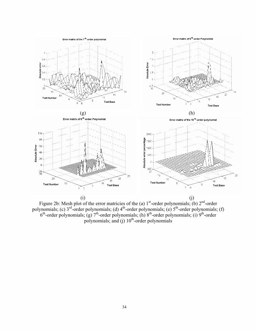
(g) (h)

(i) (j) Figure 2b: Mesh plot of the error matricies of the (a) 1st-order polynomials; (b) 2nd-order

polynomials; (c) 3rd-order polynomials; (d) 4th-order polynomials; (e) 5th-order polynomials; (f) 6th-order polynomials; (g) 7th-order polynomials; (h) 8th-order polynomials; (i) 9th-order

polynomials; and (j) 10th-order polynomials

35

Figure 3: Mesh plot of the normalised average error matrix of all test inputs using orders one to

ten. This graph is given for comparison purposes only as the 10th-order polynomials possess

larger errors compared with the other polynomials.

36

Figure 4: Mesh plot of the absolute average error matrix of all test inputs with orders one to eight

37

Figure 5: Absolute average errors of all test inputs with orders one to eight

38

0

50

100

150

0

5

100

10

20

30

40

Equation Number

Bispectrum of Fitting Error

Order

Figure 6: Mesh plot of bispectrum of the error matrix of all orders

39

0 50 100 150 200 2500

2

4

6

8

10

12

14

16

18

20Order1

Equation Number

Pow

er S

pect

rum

of F

irst-O

rder

Erro

r

0 50 100 150 200 250

0

5

10

15Order2

Equation Number

Pow

er S

pect

rum

of S

econ

d-O

rder

Erro

r

(a) (b)

0 50 100 150 200 2500

2

4

6

8

10

12

14

16

18Order3

Equation Number

Pow

er S

pect

rum

of T

hird

-Ord

er E

rror

0 50 100 150 200 250

0

2

4

6

8

10

12Order4

Equation Number

Pow

er S

pect

rum

of F

ourth

-Ord

er E

rror

(c) (d)

0 50 100 150 200 2500

2

4

6

8

10

12Order5

Equation Number

Pow

er S

pect

rum

of F

ith-O

rder

Erro

r

0 50 100 150 200 250

0

2

4

6

8

10

12Order6

Equation Number

Pow

er S

pect

rum

of S

ixth

-Ord

er E

rror

(e) (f)

Figure 7a: The power spectra of the (a) 1st-order polynomials; (b) 2nd-order polynomials; (c) 3rd-order polynomials; (d) 4th-order polynomials; (e) 5th-order polynomials; (f) 6th-order polynomials; (g) 7th-order polynomials; (h) 8th-order polynomials; (i) 9th-order polynomials; and (j) 10th-order

polynomials

40

0 50 100 150 200 2500

2

4

6

8

10

12Order7

Equation Number

Pow

er S

pect

rum

of S

even

th-O

rder

Erro

r

0 50 100 150 200 2500

1

2

3

4

5

6

7

8Order8

Equation Number

Pow

er S

pect

rum

of E

ight

h-O

rder

Erro

r

(g) (h)

0 50 100 150 200 2500

2

4

6

8

10

12

14

16Order9

Equation Number

Pow

er S

pect

rum

of N

inth

-Ord

er E

rror

0 50 100 150 200 250

0

1

2

3

4

5

6

7

8

9

10Order10

Equation Number

Pow

er S

pect

rum

of T

enth

-Ord

er E

rror

(i) (j)

Figure 7b: The power spectra of the (a) 1st-order polynomials; (b) 2nd-order polynomials; (c) 3rd-order polynomials; (d) 4th-order polynomials; (e) 5th-order polynomials; (f) 6th-order polynomials; (g) 7th-order polynomials; (h) 8th-order polynomials; (i) 9th-order polynomials; and (j) 10th-order

polynomials

41

Appendix I: Best-fit polynomials for assessing aggregate characteristics

y4 = 1015(0.0040x39 − 0.0308x3

8 + 0.1062x37 − 0.2132x3

6 + 0.2750x35 − 0.2363x3

4 + 0.1353x3

3 − 0.0498x32 + 0.0107x3 − 0.0010 (with error of 0.88%)

(8)

y5 = 1013(−0.0003x38 + 0.0023x3

7 − 0.0069x36 + 0.0120x3

5 − 0.0131x34 + 0.0091x3

3 − 0.0040x3

2 + 0.0010x3 − 0.0001 (with error of 0.12%)

(9)

y6 = 1013(0.0014x38 − 0.0096x3

7 + 0.0292x36 − 0.0508x3

5 + 0.0552x34 − 0.0383x3

3 + 0.0166x3

2 − 0.0041x3 + 0.0004 (with error of 0.60%)

(10)

y7 = 1015(0.0006x39 − 0.0045x3

8 + 0.0156x37 − 0.0315x3

6 + 0.0407x35 − 0.0350x3

4 − 0.0201x3

3 − 0.0074x32 + 0.0016x3 − 0.0002 (with error of 0.42%)

(11)

y8 = 1015(0.0050x310 − 0.0361x3

9 + 0.1113x38 − 0.1887x3

7 + 0.1821x36 − 0.0813x3

5 − 0.0192x3

4 + 0.0479x33 − 0.0280x3

2 + 0.0078x3 − 0.0009) (with error of 2.18%)

(12)

y9 = 1015(0.0069x310 − 0.0362x3

9 + 0.0489x38 + 0.1012x3

7 − 0.4791x36 + 0.8371x3

5 − 0.8491x3

4 + 0.5413x33 − 0.2150x3

2 + 0.0489x3 − 0.0049) (with error of 2.13%)

(13)

y10 = 1015(0.0254x39 − 0.1964x3

8 + 0.6746x37 − 1.3509x3

6 + 1.7377x35 − 1.4890x3

4 + 0.8499x3

3 − 0.3116x32 + 0.0666x3 − 0.0063 (with error of 5.22%)

(14)

y11 = 1011(0.0327x34 − 0.1157x3

3 + 0.1534x32 − 0.0902x3 + 0.0199) (with error of

7.77%)

(15)

y12 = −4.4200x3 + 4.5739 (with error of 18.83%)

(16)

y13 = 1013(0.0518x38 − 0.3616x3

7 + 1.1038x36 − 1.9237x3

5 + 2.0940x34 − 1.4578x3

3 + 0.6339x3

2 − 0.1574x3 + 0.0171 (with error of 2.40%)

(17)

y14 = –16.4255x32 + 25.1580x3 – 8.7004 (with error of 22.46%)

(18)

y15 = 1013(0.0630x38 − 0.4399x3

7 + 1.3420x36 − 2.3378x3

5 + 2.5435x34 − 1.7699x3

3 + 0.7692x3

2 − 0.1909x3 + 0.0207 (with error of 3.93%)

(19)

y16 = 1013(0.0292x38 − 0.2041x3

7 + 0.6238x36 − 1.0886x3

5 + 1.1866x34 − 0.8272x3

3 + 0.3602x3

2 − 0.0896x3 + 0.0097 (with error of 4.39%)

(20)

y17 = 1011(−0.0209x37 + 0.1286x3

6 − 0.3396x35 + 0.4978x3

4 − 0.4373x33 + 0.2304x3

2 − 0.0674x3 + 0.0084) (with error of 11.74%)

(21)

y18 = 1015(-0.0047x310 + 0.0372x3

9 − 0.1327x38 + 0.2782x3

7 − 0.3783x36 + 0.3480x3

5 − 0.2185x3

4 + 0.0920x33 − 0.0246x3

2 + 0.0037x3 − 0.0002) (with error of 3.80%)

(22)

y19 = 1015(0.0073x39 − 0.0564x3

8 + 0.1941x37 − 0.3890x3

6 + 0.5008x35 − 0.4296x3

4 + (23)

42

0.2455x33 − 0.0901x3

2 + 0.0193x3 − 0.0018 (with error of 4.28%) y20 = 1015(0.0274x3

9 − 0.2126x38 + 0.7339x3

7 − 1.4764x36 + 1.9082x3

5 − 1.6431x34 +

0.9425x33 − 0.3474x3

2 + 0.0746x3 − 0.0071 (with error of 2.92%)

(24)

y21 = −1013(0.0127x38 − 0.0896x3

7 + 0.2759x36 − 0.4853x3

5 + 0.5331x34 − 0.3746x3

3 + 0.1644x3

2 − 0.0412x3 + 0.0045 (with error of 21.75%)

(25)

y22 = 1015(0.0425x39 − 0.3300x3

8 + 1.1387x37 − 2.2908x3

6 + 2.9604x35 − 2.5489x3

4 + 1.4621x3

3 − 0.5388x32 + 0.1158x3 − 0.0110 (with error of 13.52%)

(26)

y23 = −1013(0.1656x38 − 1.1553x3

7 + 3.5247x36 − 6.1401x3

5 + 6.6803x34 − 4.64836x3

3 + 2.0201x3

2 − 0.5013x3 + 0.0544 (with error of 21.93%)

(27)

y5 = 1013(0.0029x48 − 0.0201x4

7 + 0.0612x46 − 0.1068x4

5 + 0.1162x44 − 0.0809x4

3 + 0.0352x4

2 − 0.0087x4 + 0.0009) (with error of 0.75%)

(28)

y6 = 1015(−0.0004x410 + 0.0029x4

9 − 0.0092x48 + 0.0160x4

7 − 0.0163x46 + 0.0087x4

5 − 0.0003x4

4 − 0.0028x43 + 0.0018x4

2 − 0.0005x4 + 0.0001) (with error of 0.34%)

(29)

y7 = 1013(0.0005x48 − 0.0033x4

7 + 0.0100x46 − 0.0174x4

5 + 0.0190x44 − 0.0132x4

3 + 0.0058x4

2 − 0.0014x4 + 0.0002) (with error of 0.87%)

(30)

y8 = 1015(0.0167x410 − 0.1258x4

9 + 0.4148x48 − 0.7820x4

7 + 0.9156x46 − 0.6690x4

5 + 0.2776x4

4 − 0.0353x43 − 0.0218x4

2 + 0.0106x4 − 0.0015) (with error of 1.21%)

(31)

y9 = −1013(0.0320x48 − 0.2230x4

7 + 0.6799x46 − 1.1839x4

5 + 1.2873x44 − 0.8952x4

3 + 0.3887x4

2 − 0.0964x4 + 0.0105) (with error of 9.90%)

(32)

y10 = −1013(0.0549x48 − 0.3833x4

7 + 1.1690x46 − 2.0360x4

5 + 2.2144x44 − 1.5402x4

3 + 0.6690x4

2 − 0.1659x4 + 0.0180) (with error of 10.86%)

(33)

y11 = 109(0.0048x46 − 0.0252x4

5 + 0.0552x44 − 0.0644x4

3 + 0.0422x42 + 0.0148x4 +

0.0021) (with error of 3.57%)

(34)

y12 = −1013(0.0757x48 − 0.5282x4

7 + 1.6112x46 − 2.8066x4

5 + 3.0529x44 − 2.1238x4

3 + 0.9227x4

2 − 0.2289x4 + 0.0248) (with error of 9.28%)

(35)

y13 = 1011(−0.0487x47 + 0.2997x4

6 − 0.7894x45 + 1.1540x4

4 − 1.0112x43 + 0.5311x4

2 − 0.1548x4 + 0.0193) (with error of 8.44%)

(36)

y14 = 1015(0.0053x49 − 0.0408x4

8 + 0.1393x47 − 0.2773x4

6 + 0.3546x45 − 0.3019x4

4 + 0.1712x4

3 − 0.0623x42 + 0.0132x4 − 0.0012) (with error of 3.88%)

(37)

y15 = 103(0.4151x43 − 1.1333x4

2 + 1.0240x4 − 0.3056) (with error of 11.45%)

(38)

43

y16 = 1015(−0.0088x410 + 0.0645x4

9 − 0.2065x48 + 0.3729x4

7 − 0.4066x46 + 0.2572x4

5 − 0.0661x4

4 − 0.0264x43 + 0.0278x4

2 − 0.0090x4 + 0.0011) (with error of 6.11%)

(39)

y17 = 1013(0.0245x48 −0.1708x4

7 + 0.5203x46 − 0.9051x4

5 + 0.9833x44 − 0.6831x4

3 + 0.2964x4

2 − 0.0734x4 + 0.0080) (with error of 11.96%)

(40)

y18 = 1011(−0.0144x47 + 0.0885x4

6 − 0.2334x45 + 0.3416x4

4 − 0.2997x43 + 0.1576x4

2 − 0.0460x4 + 0.0058) (with error of 13.67%)

(41)

y19 = 1015(0.0149x49 − 0.1171x4

8 + 0.4078x47 − 0.8282x4

6 + 1.0804x45 − 0.9391x4

4 + 0.5439x4

3 − 0.2024x42 + 0.0439x4 − 0.0042) (with error of 3.87%)

(42)

y20 1015(0.0060x49 − 0.0469x4

8 + 0.1629x47 − 0.3302x4

6 + 0.4301x45 − 0.3731x4

4 + 0.2157x4

3 − 0.0801x42 + 0.0173x4 − 0.0017) (with error of 11.26%)

(43)

y21 = −1013(0.1083x48 −0.7569x4

7 + 2.3119x46 − 4.0320x4

5 + 4.3915x44 − 3.0589x4

3 + 1.3307x4

2 − 0.3305x4 + 0.0359) (with error of 15.56%)

(44)

y22 = −1013(0.1053x48 −0.7356x4

7 + 2.2472x46 − 3.9198x4

5 + 4.2699x44 − 2.9746x4

3 + 1.2942x4

2 − 0.3215x4 + 0.0349) (with error of 16.09%)

(45)

y23 = −109(0.0412x46 − 0.2189x4

5 + 0.4836x44 − 0.5693x4

3 + 0.3765x42 + 0.1327x4 +

0.0195) (with error of 25.29%)

(46)

y6 = 1015(0.0006x59 − 0.0041x5

8 + 0.0015x57 − 0.0169x5

6 + 0.0127x55 − 0.0020x5

4 − 0.0046x5

3 + 0.0041x52 − 0.0015x5 + 0.0002) (with error of 0.08%)

(47)

y7 = 1015(0.0004x59 − 0.0026x5

8 + 0.0086x57 − 0.0162x5

6 + 0.0192x55 − 0.0148x5

4 + 0.0073x5

3 − 0.0022x52 + 0.0004x5) (with error of 0.31%)

(48)

y8 = 1015(0.0071x59 − 0.0475x5

8 + 0.1333x57 − 0.1975x5

6 + 0.1511x55 − 0.0281x5

4 − 0.0502x5

3 + 0.0461x52 + 0.0166x5 + 0.0023) (with error of 1.38%)

(49)

y9 = 1012(0.0561x57 − 0.3624x5

6 + 1.0022x55 − 1.5392x5

4 + 1.4179x53 − 0.7835x5

2 + 0.2404x5 − 0.0316) (with error of 2.69%)

(50)

y10 = 1015(0.0068x59 − 0.0398x5

8 + 0.0858x57 − 0.0546x5

6 − 0.1022x55 + 0.2561x5

4 − 0.2557x5

3 + 0.1394x52 − 0.0408x5 + 0.0051) (with error of 5.91%)

(51)

y11 = 105(0.3563x54−1.3260x5

3 + 1.8491x52 – 1.1451x5 + 0.2657 (with error of

8.09%)

(52)

y12 = 1015(0.0080x59 − 0.0535x5

8 + 0.1506x57 − 0.2247x5

6 + 0.1751x55 − 0.0379x5

4 − 0.0516x5

3 + 0.0496x52 − 0.0181x5 + 0.0025) (with error of 13.20%)

(53)

y13 = 1012(0.0038x57 − 0.0237x5

6 + 0.0642x55 − 0.0963x5

4 + 0.0867x53 − 0.0468x5

2 + (54)

44

0.0140x5 − 0.0018) (with error of 7.50%) y14 = −35.3738x5

2 – 59.2782x5 − 23.8713 (with error of 22.59%)

(55)

y15 = 1012(0.0346x57 − 0.2231x5

6 + 0.6161x55 − 0.9447x5

4 + 0.8689x53 − 0.4794x5

2 + 0.1469x5 − 0.0193) (with error of 8.65%)

(56)

y16 = –1012(0.0323x57 − 0.2082x5

6 + 0.5755x55 − 0.8835x5

4 + 0.8136x53 − 0.4494x5

2 + 0.1379x5 − 0.0181) (with error of 6.34%)

(57)

y17 = –1012(0.0430x57 − 0.2779x5

6 + 0.7687x55 − 1.1808x5

4 + 1.0880x53 − 0.6013x5

2 + 0.1846x5 − 0.0243) (with error of 12.59%)

(58)

y18 = 107(−0.3842x55 + 1.7913x5

4−3.3391x53 + 3.1106x5

2 – 1.4481x5 + 0.2695 (with error of 12.11%)

(59)

y19 = 1015(0.0044x59 − 0.0320x5

8 + 0.1011x57 − 0.1816x5

6 + 0.2021x55 − 0.1418x5

4 + 0.0602x5

3 − 0.0133x52 + 0.0007x5 + 0.0002) (with error of 2.65%)

(60)

y20 = 103(−1.2437x53 + 3.4712x5

2 – 3.2274x5 + 1.0005 (with error of 19.14%)

(61)

y21 = 1015(−0.0191x58 + 0.1406x5

7 − 0.4526x56 + 0.8321x5

5 − 0.9559x54 + 0.7026x5

3 − 0.3227x5

2 + 0.0847x5 − 0.0097) (with error of 12.57%)

(62)

y22 = 1015(−0.0193x58 + 0.1653x5

7 − 0.5309x56 + 0.9738x5

5 − 1.1162x54 + 0.8186x5

3 − 0.3751x5

2 + 0.0982x5 − 0.0112) (with error of 12.18%)

(63)

y23= 1015(−0.0225x58 + 0.1653x5

7 − 0.5309x56 + 0.9738x5

5 − 1.1162x54 + 0.8186x5

3 − 0.3751x5

2 + 0.0982x5 − 0.0112) (with error of 13.13%)

(64)

y7 = 1012(0.0029x67 − 0.0188x6

6 + 0.0518x65 − 0.0796x6

4 + 0.0733x63 − 0.0404x6

2 + 0.0124x6 − 0.0016) (with error of 0.73%)

(65)

y8 = 1015(0.0017x68 − 0.0125x6

7 + 0.0403x66 − 0.0743x6

5 + 0.0855x64 − 0.0630x6

3 + 0.0290x6

2 − 0.0076x6 + 0.0009) (with error of 1.45%)

(66)

y9 = –1012(0.0554x67 − 0.3575x6

6 + 0.9876x65 − 1.5153x6

4 + 1.3944x63 − 0.7696x6

2 + 0.2359x6 − 0.0310) (with error of 8.53%)

(67)

y10 = –1012(0.0839x67 − 0.5407x6

6 + 1.4937x65 − 2.2916x6

4 + 2.1086x63 − 1.1636x6

2 + 0.3566x6 – 0.0468) (with error of 6.84%)

(68)

y11 = −1015(0.0008x69 − 0.0005x6

8 − 0.0199x67 + 0.0895x6

6 − 0.1873x65 + 0.2304x6

4 − 0.1765x6

3 + 0.0833x62 − 0.0223x6 + 0.0026) (with error of 6.29%)

(69)

y12 = –1012(0.0822x67 − 0.5300x6

6 + 1.4642x65 − 2.2464x6

4 + 2.0672x63 − 1.1409x6

2 (70)

45

+ 0.3497x6 − 0.0459) (with error of 16.97%) y13 = 105(−0.0584x6

4 + 0.2191x63 − 0.3080x6

2 + 0.1925x6 − 0.0451) (with error of 14.53%)

(71)

y14 = 108(0.0241x65 − 0.1126x6

4 + 0.2106x63 − 0.1968x6

2 + 0.0919x6 − 0.0172) (with error of 13.02%)

(72)

y15 = –1012(0.0496x67 − 0.3199x6

6 + 0.8838x65 − 1.3562x6

4 + 1.2482x63 − 0.6890x6

2 + 0.2112x6 − 0.0277) (with error of 10.54%)

(73)

y16 = 1015(0.0041x68 − 0.0301x6

7 + 0.0966x66 − 0.1772x6

5 + 0.2031x64 − 0.1489x6

3 + 0.0682x6

2 − 0.0179x6 + 0.0020) (with error of 5.52%)

(74)

y17 = 1015(0.0098x69 − 0.0453x6

8 + 0.0356x67 + 0.2028x6

6 − 0.6620x65 + 0.9574x6

4 − 0.7988x6

3 + 0.3975x62 − 0.1102x6 + 0.0132) (with error of 12.22%)

(75)

y18 = –1012(0.0064x67 − 0.0412x6

6 + 0.1140x65 − 0.1749x6

4 + 0.1611x63 − 0.0889x6

2 + 0.0273x6 − 0.0036) (with error of 12.78%)

(76)

y19 = 1010(0.0475x66 − 0.2638x6

5 + 0.6098x64 − 0.7515x6

3 + 0.5207x62 −0.1923x6 +

0.0296) (with error of 7.01%)

(77)

y20 = 1015(0.0027x69 − 0.0302x6

8 + 0.1397x67 − 0.3608x6

6 + 0.5812x65 − 0.6105x6

4 + 0.4203x6

3 − 0.1836x62 + 0.0463x6 − 0.0051) (with error of 3.32%)

(78)

y21 = 2.4420x6 + 2.4079 (with error of 25.78%)

(79)

y22 = −2.1765x6 + 2.1675 (with error of 24.75%)

(80)

y23 = 1015(0.0303x68 − 0.2223x6

7 + 0.7128x66 − 1.3059x6

5 + 1.4948x64 − 1.0947x6

3 + 0.5009x6

2 − 0.1309x6 + 0.0150) (with error of 2.07%)

(81)

y8= 1015(0.0278x78 − 0.1869x7

7 + 0.5340x76 − 0.8350x7

5 + 0.7613x74 − 0.3899x7

3 + 0.0887x7

2 + 0.0041x7 − 0.0041) (with error of 6.59)

(82)

y9= −1015(0.0475x78 − 0.3243x7

7 + 0.9443x76 − 1.5186x7

5 + 1.4493x74 − 0.8109x7

3 + 0.2363x7

2 − 0.0207x7 − 0.0031) (with error of 13.61)

(83)

y10 = 1013(−0.0347x76 + 0.2045x7

5 − 0.5030x74 + 0.6597x7

3 − 0.4866x72 + 0.1915x7 −

0.0314) (with error of 45.14%)

(84)

y11= −1015(0.0300x78 − 0.1963x7

7 + 0.5384x76 − 0.7888x7

5 + 0.6369x74 − 0.2390x7

3 − 0.0116x7

2 + 0.0396x7 − 0.0093) (with error of 16.46)

(85)

y12= −1015(0.0753x78 − 0.5011x7

7 + 1.4085x76 − 2.1465x7

5 + 1.8699x74 − 0.8647x7

3 + (86)

46

0.1263x72 + 0.0487x7 − 0.0164) (with error of 23.03)

y13 = 1013(−0.0350x7

6 + 0.2064x75 − 0.5078x7

4 + 0.6663x73 − 0.4918x7

2 + 0.1936x7 − 0.0317) (with error of 21.35%)

(87)

y14 = −1015(−0.0333x78 + 0.2190x7

7 − 0.6037x76 + 0.8903x7

5 − 0.7268x74 + 0.2808x7

3 + 0.0060x7

2 − 0.0424x7 + 0.0102) (with error of 30.28%)

(88)

y15 = −1013(−0.0413x76 + 0.2442x7

5 − 0.6011x74 + 0.7891x7

3 − 0.582872 + 0.2295x7 −

0.0377) (with error of 15.42%)

(89)

y16 = 108(0.0541x74 − 0.2135x7

3 + 0.3162x72 − 0.2080x7 + 0.0513) (with error of

22.68%)

(90)

y17 = 108(−0.0270x74 + 0.1053x7

3 − 0.1543x72 + 0.1004x7 − 0.0245) (with error of

9.58%)

(91)

y18 = −1013(−0.0291x76 + 0.1722x7

5 − 0.4242x74 + 0.5573x7

3 − 0.411872 + 0.1623x7 −

0.0267) (with error of 15.13%)

(92)

y19 = –1012(0.0243x67 − 0.1573x6

6 + 0.4359x65 − 0.6707x6

4 + 0.6189x63 − 0.3425x6

2 + 0.1053x6 − 0.0139) (with error of 7.09%)

(93)

y20 = 1015(−0.0158x78 + 0.0999x7

7 − 0.2604x76 + 0.3477x7

5 − 0.2248x74 + 0.0172x7

3 + 0.0702x7

2 − 0.0419x7 + 0.0079 (with error of 4.47%)

(94)

y21 = 103(–0.7980x72 + 1.5607x7 – 0.7627) (with error of 27.74%)

(95)

y22 = 103(–0.6919x72 + 1.3519x7 – 0.6601) (with error of 26.65%)

(96)

y23 = 1014(0.0551x77 − 0.3837x7

6 + 1.1445x75 − 1.8964x7

4 + 1.8853x73 − 1.1245x7

2 + 0.3726x7 − 0.0529) (with error of 1.25%)

(97)

y9 = 1013(0.0544x87 − 0.3530x8

6 + 0.9785x85 − 1.5013x8

4 + 1.3759x83 − 0.7528x8

2 + 0.2275x8 − 0.0293) (with error of 15.16%)

(98)

y10 = 1013(0.0290x87 − 0.1880x8

6 + 0.5204x85− 0.7973x8

4 + 0.7297x83 − 0.3987x8

2 + 0.1203x8 − 0.0155) (with error of 8.74%)

(99)

y11 = 1010(0.1902x86 − 1.0453x8

5 + 2.3820x84 − 2.8793x8

3 + 1.9454x82 − 0.6958x8 +

0.1028) (with error of 9.74%)

(100)

y12 = 1013(0.0638x87 − 0.4140x8

6 + 1.1472x85 − 1.7593x8

4 + 1.6117x83 − 0.8814x8

2 + 0.2663x8 − 0.0342) (with error of 3.68%)

(101)

y13 = 1010(0.3883x86 − 2.1374x8

5 + 4.8792x84 − 5.9078x8

3 + 3.9983x82 − 1.4324x8 + (102)

47

0.2119) (with error of 15.42%) y14 = 108(0.3920x8

5 − 1.7743x84 + 3.1896x8

3 − 2.8429x82 + 1.2542x8 − 0.2186) (with

error of 19.47%)

(103)

y15 = 1010(0.1835x86 − 1.0083x8

5 + 2.2972x84 − 27761x8

3 + 1.8753x82 − 0.6706x8 +

0.0990) (with error of 6.40%)

(104)

y16 = 1015(−0.0002x88 + 0.0011x8

7 − 0.0018x86 + 0.0001x8

5 + 0.0038x84 − 0.0056x8

3 + 0.0038x8

2 − 0.0013x8 + 0.0002) (with error of 11.99%)

(105)

y17 = 1015(−0.0017x88 + 0.012x8

7 − 0.0368x86 + 0.0638x8

5 − 0.06878x84 − 0.0470x8

3 − 0.0199x8

2 + 0.0048x8 − 0.0005) (with error of 5.99%)

(106)

y18 = −108(0.1673x85 − 0.7569x8

4 + 1.3606x83 − 1.2127x8

2 + 0.5350x8 − 0.0932) (with error of 13.51%)

(107)

y19 = 0.7973x8 − 0.1898 (with error of 14.88%)

(108)

y20 = −9.1630x82 + 14.0679x8 − 4.1517 (with error of 18.57%)

(109)

y21 = 1013(0.2521x87 − 1.6372x8

6 + 4.5410x85 − 6.9704x8

4 + 6.3915x83 − 3.4987x8

2 + 1.0578x8 − 0.1361) (with error of 13.22%)

(110)

y22 = 1015(−0.0013x88 + 0.0125x8

7 − 0.0491x86 + 0.1068x8

5 − 0.1413x84 − 0.1172x8

3 − 0.0596x8

2 + 0.0171x8 − 0.0021) (with error of 9.47%)

(111)

y23 = 1015(−0.0236x88 + 0.1768x8

7 − 0.5789x86 + 1.0802x8

5 − 1.2555x84 − 0.9305x8

3 − 0.4293x8

2 + 0.1126x8 − 0.0129) (with error of 10.24%)

(112)

y10 = 107(0.0230x910 − 0.1572x9

9 + 0.4755x98 − 0.8345x9

7 + 0.9371x96 − 0.7001x9

5 + 0.3497x9

4 − 0.1140x93 + 0.0228x9

2 − 0.0024x9 + 0.0001) (with error of 1.87%)

(113)

y11 = 1010(0.0315x97 − 0.1476x9

6 + 0.2832x95− 0.2850x9

4 + 0.1599x93 − 0.0486x9

2 + 0.0071x9 − 0.0003) (with error of 5.05%)

(114)

y12 = 1010(0.0519x910 − 0.3551x9

9 + 1.0733x98 − 1.8819x9

7 + 2.1119x96 − 2.5767x9

5 + 0.7870x9

4 − 0.2564x93 + 0.0512x9

2 − 0.0055x9 + 0.0002) (with error of 2.42%)

(115)

y13 = 1010(−0.0017x910 + 0.0116x9

9 − 0.0354x98 + 0.0627x9

7 − 0.0711x96 + 0.0536x9

5 − 0.0270x9

4 + 0.0089x93 − 0.0018x9

2 + 0.0002x9) (with error of 0.23%)

(116)

y14 = 1010(−0.0388x910 + 0.2659x9

9 − 0.8043x98 + 1.4116x9

7 − 1.5855x96 + 1.1847x9

5 − 0.5919x9

4 + 0.1930x93 − 0.0386x9

2 + 0.0041x9 − 0.0002) (with error of 15.84%)

(117)

y15 = 1010(−0.0171x910 + 0.1170x9

9 − 0.3534x98 + 0.6194x9

7 − 0.6949x96 + 0.5186x9

5 (118)

48

− 0.2588x94 + 0.0843x9

3 − 0.0168x92 + 0.0018x9 − 0.0001) (with error of 2.44%)

y16 = 1010(−0.0034x9

10 + 0.0232x99 − 0.0693x9

8 + 0.1200x97 − 0.1330x9

6 + 0.0981x95

− 0.0484x94 + 0.0156x9

3 − 0.0031x92 + 0.0003x9) (with error of 7.44%)

(119)

y17 = 1010(−0.0433x910 + 0.2955x9

9 − 0.8915x98 + 1.5603x9

7 − 1.7479x96 + 1.3027x9

5 − 0.6492x9

4 + 0.2112x93 − 0.0421x9

2 + 0.0045x9 − 0.0002) (with error of 6.34%)

(120)

y18 = 1010(−0.0029x910 + 0.0198x9

9 − 0.0590x98 + 0.1022x9

7 − 0.1132x96 + 0.0834x9

5 − 0.0411x9

4 + 0.0132x93 − 0.0026x9

2 + 0.0003x9) (with error of 8.15%)

(121)

y19 = 108(0.0251x99 − 0.1519x9

8 + 0.3990x97 − 0.5947x9

6 + 0.5513x95 − 0.3269x9

4 + 0.1224x9

3 − 0.0273x92 + 0.0032x9 − 0.0001) (with error of 4.21%)

(122)

y20 = 108(−0.0284x99 + 0.1717x9

8 − 0.4506x97 + 0.6710x9

6 − 0.6215x95 + 0.3682x9

4 − 0.1377x9

3 + 0.0307x92 − 0.0036x9 + 0.0002) (with error of 16.73%)

(123)

y21 = 1010(−0.0296x910 + 0.2031x9

9 − 0.6153x98 + 1.0816x9

7 − 1.2168x96 + 0.9106x9

5 − 0.4556x9

4 + 0.1488x93 − 0.0298x9

2 + 0.0032x9 − 0.0001) (with error of 24.94%)

(124)

y22 = 1010(−0.0333x910 + 0.2284x9

9 − 0.6916x98 + 1.2152x9

7 − 1.3665x96 + 1.0222x9

5 − 0.5112x9

4 + 0.1669x93 − 0.0334x9

2 + 0.0036x9 − 0.0001) (with error of 20.73%)

(125)

y23 = 105(0.1447x97 − 0.6583x9

6 + 1.2356x95− 1.2269x9

4 + 0.6840x93 − 0.2080x9

2 + 0.0303x9 − 0.0015) (with error of 26.32%)

(126)

y11 = 109(0.0243x108 − 0.1515x10

7 + 0.4067x106 − 0.6130x10

5 + 0.5649x104 −

0.3238x103 + 0.1116x10

2 − 0.0207x10 + 0.0015) (with error of 6.76%)

(127)

y12 = 1011(0.0263x109 − 0.1879x10

8 + 0.5900x107 − 1.0664x10

6 + 1.2193x105 −

0.9110x104 + 0.4421x10

3 − 0.1332x102 + 0.0222x10 − 0.0015) (with error of 0.82%)

(128)

y13 = 1011(−0.0708x109 + 0.5065x10

8 − 1.5922x107 + 2.8807x10

6 − 3.2969x105 +

2.4655x104 − 1.1977x10

3 + 0.3611x102 − 0.0603x10 + 0.0041) (with error of 10.43%)

(129)

y14 = 1011(−0.0434x109 + 0.3108x10

8 − 0.9772x107 + 1.7686x10

6 − 2.0249x105 +

1.5148x104 − 0.7361x10

3 + 0.2220x102 − 0.0371x10 + 0.0025) (with error of 14.09%)

(130)

y15 = 1011(−0.0161x109 + 0.1149x10

8 − 0.3613x107 + 0.6540x10

6 − 0.7488x105 +

0.5601x104 − 0.2722x10

3 + 0.0821x102 − 0.0137x10 + 0.0009) (with error of 4.53%)

(131)

y16 = 1017(0.0042x1010 − 0.0339x10

9 + 0.1221x108 − 0.2582x10

7 + 0.3540x106 −

0.3278x105 + 0.2069x10

4 − 0.0875x103 + 0.0235x10

2 − 0.0036x10 + 0.0002) (with error of 60.38%)

(132)

y17 = 1011(−0.0108x109 + 0.0770x10

8 − 0.2410x107 + 0.4343x10

6 − 0.4952x105 + (133)

49

0.3689x104 − 0.1786x10

3 + 0.0537x102 − 0.0089x10 + 0.0006) (with error of 8.88%)

y18 = 107(0.0071x10

7 − 0.0395x106 + 0.0917x10

5− 0.1151x104 + 0.0839x10

3 − 0.0350x10

2 + 0.0076x10 − 0.0006) (with error of 11.48%)

(134)

y19 = 1.3676x102 – 1.8268x10 + 1.0608 (with error of 22.07%)

(135)

y20 = –107(0.0175x107 − 0.0939x10

6 + 0.2113x105− 0.2578x10

4 + 0.1828x103 −

0.0744x102 + 0.0157x10 − 0.0013) (with error of 16.67%)

(136)

y21 = 5.1263x103 − .95237x10

2 + 5.4239x10 − 0.7038 (with error of 22.89%)

(137)

y22 = 99.3243x104 − 269.4538x10

3 + 256.4748x102 − 96.8644x10 + 10.8853 (with error

of 20.29%)

(138)

y23 = 107(0.0383x107 − 0.1983x10

6 + 0.4317x105− 0.5092x10

4 + 0.3492x103 −

0.1376x102 + 0.0282x10 − 0.0022) (with error of 8.58%)

(139)

y12 = 1011(0.0154x1110 − 0.1081x11

9 + 0.3357x118 − 0.6034x11

7 + 0.6913x116 −

0.5236x115 + 0.2625x11

4 − 0.0845x113 + 0.0163x11

2) (with error of 3.86%)

(140)

y13 = 103(0.0858x114 − 0.2356x11

4 + 0.2342x113 − 0.10031x11

2 + 0.0177x11 − 0.0007) (with error of 10.27%)

(141)

y14 = 1011(−0.0140x1110 + 0.0984x11

9 − 0.3058x118 + 0.5500x11

7 − 0.6307x116 +

0.4781x115 − 0.2399x11

4 + 0.0773x113 − 0.0149x11

2 + 0.0015x11) (with error of 14.17%)

(142)

y15 = 1011(0.0108x1110 − 0.0757x11

9 + 0.2335x118 − 0.4170x11

7 + 0.4747x116 −

0.3571x115 + 0.1779x11

4 − 0.0569x113 + 0.0109x11

2 − 0.0011x11 − 0.0001) (with error of 9.54%)

(143)

y16 = 107(−0.0596x118 + 0.3193x11

7 − 0.7239x116 + 0.8994x11

5 − 0.6607x114 +

0.2876x113 − 0.0698x11

2 + 0.0081x112 − 0.0003) (with error of 5.38%)

(144)

y17 = 109(0.0326 x119 − 0.2036x11

8 + 0.5515x117 − 0.8448x11

6 + 0.7999x115 −

0.4795x114 + 0.1785x11

3 − 0.0385x112 + 0.0041x11

2 − 0.0002) (with error of 8.12%)

(145)

y18 = 1011(0.0078x1110 − 0.0539x11

9 + 0.1655x118 − 0.2939x11

7 + 0.3327x116 −

0.2490x115 + 0.1234x11

4 − 0.0393x113 + 0.0075x11

2 − 0.0007x11) (with error of 6.57%)

(146)

y19 = 1011(0.0035x1110 − 0.0250x11

9 + 0.0779x118 − 0.1406x11

7 + 0.1617x116 −

0.1229x115 + 0.0619x11

4 − 0.0200x113 + 0.0039x11

2 − 0.0004x11) (with error of 0.95%)

(147)

50

y20 = 1011(0.0004x1110 − 0.0031x11

9 + 0.0107x118 − 0.0209x11

7 + 0.0258x116 −

0.0209x115 + 0.0111x11

4 − 0.0038x113 + 0.0008x11

2 − 0.0001x11) (with error of 5.29%)

(148)

y21 = 1011(0.0291x1110 − 0.2039x11

9 + 0.6291x118 − 1.1236x11

7 + 1.2792x116 −

0.9627x115 + 0.4797x11

4 − 0.1536x113 + 0.0294x11

2 − 0.0029x11 + 0.0001) (with error of 36.41%)

(149)

y22 = −9.2682x114 + 18.0352x11

3 − 11.1493x112 + 2.5850x11 − 0.1184 (with error of

21.74%)

(150)

y23 = 1011(−0.0329x1110 + 0.2297x11

9 − 0.7078x118 + 1.2625x11

7 − 1.4355x116 +

1.0790x115 − 0.5369x11

4 + 0.1717x113 − 0.0328x11

2 + 0.0032x11 − 0.0001) (with error of 21.83%)

(151)

y13 = −106 (0.1338x127 − 0.6826x12

6 + 1.4616x125 − 1.6956x12

4 + 1.1437x123 −

0.4439x122 + 0.0901x12 − 0.0071) (with error of 10.43%)

(152)

y14 = 1017(0.0377x1210 − 0.2963x12

9 + 1.0389x128 − 2.1348x12

7 + 2.8419x126 −

2.5549x125 + 1.5658x12

4 − 0.6430x123 + 0.1681x12

2 − 0.0250x12 + 0.0016) (with error of 7.41%)

(153)

y15 = 107 (−0.1274x128 + 0.7601x12

7 − 1.9542x126 + 2.8201x12

5 − 2.4890x124 +

1.3680x123 − 0.4532x12

2 + 0.0815x12 − 0.0059) (with error of 4.07%)

(154)

y16 = 106 (0.0158x127 − 0.0796x12

6 + 0.1680x125 − 0.1920x12

4 + 0.1275x123 −

0.0487x122 + 0.0097x12 − 0.0008) (with error of 11.86%)

(155)

y17 = 106 (0.0706x127 − 0.3612x12

6 + 0.7763x125 − 0.9054x12

4 + 0.6148x123 −

0.2405x122 + 0.0492x12 − 0.0039) (with error of 8.88%)

(156)

y18 = −106 (0.1172x127 − 0.6081x12

6 + 1.3247x125 − 1.5640x12

4 + 1.0738x123 −

0.4241x122 + 0.0875x12 − 0.0070) (with error of 11.48%)

(157)

y19 = 1.6289x122 – 2.1370x12 + 1.1277 (with error of 22.66%)

(158)

y20 = 57.8441x124 − 158.8260x12

3 + 151.9245x122 – 57.4083x12 + 7.2865 (with error

of 16.66%)

(159)

y21 = 0.2918x12 − 0.0279 (with error of 25.06%)

(160)

y22 = 0.2494x12 + 0.0045 (with error of 23.28%)

(161)

y23 = 1010(0.0388x129 − 0.2679x12

8 + 0.8121x127 − 1.4163x12

6 + 1.5619x125 −

1.1256x124 + 0.5274x12

3 − 0.1537x122 + 0.0250x12 − 0.0017) (with error of 12.90%)

(162)

51

y14 = 1011(−0.0399x1310 + 0.2525x13

9 − 0.7065x138 + 1.1482x13

7 − 1.1967x136 +

0.8319x135 − 0.3880x13

4 + 0.1188x133 − 0.0225x13

2 + 0.0023x13 − 0.0001) (with error of 3.52%)

(163)

y15 = 107(0.0206x138 − 0.0958x13

7 + 0.1882x136 − 0.2033x13

5 + 0.1313x134 −

0.0513x133 + 0.0117x13

2 − 0.0014x13 + 0.0001 (with error of 3.52%)

(164)

y16 = 1010(0.0118x139 − 0.0661x13

8 + 0.1616x137 − 0.2246x13

6 + 0.1946x135 −

0.1082x134 + 0.0382x13

3 − 0.0081x132 + 0.0009x13) (with error of 6.66%)

(165)

y17 = 107(0.1171x138 − 0.5649x13

7 + 1.1575x136 − 1.3096x13

5 + 0.8880x134 −

0.3652x133 + 0.0872x13

2 − 0.0107x13 + 0.0005 (with error of 10.54%)

(166)

y18 = 1011(−0.0053x1310 + 0.0310x13

9 − 0.0802x138 + 0.1195x13

7 − 0.1132x136 +

0.0710x135 − 0.0296x13

4 + 0.0080x133 − 0.0013x13

2 + 0.0001x13) (with error of 0.28%)

(167)

y19 = 1011(0.0068x1310 − 0.0447x13

9 + 0.1294x138 − 0.2175x13

7 + 0.2342x136 −

0.1679x135 + 0.0806x13

4 − 0.0254x133 + 0.0049x13

2 − 0.0005x13) (with error of 5.47%)

(168)

y20 =1011(0.0067x1310 − 0.0400x13

9 + 0.1059x138 − 0.1624x13

7 + 0.1591x136 −

0.1036x135 + 0.0451x13

4 − 0.0129x133 + 0.0023x13

2 − 0.0002x13) (with error of 12.50%)

(169)

y21 = 1011(0.1523x1310 − 0.9639x13

9 + 2.6974x138 − 4.3858x13

7 + 4.5728x136 −

3.1801x135 + 1.4840x13

4 − 0.4543x133 + 0.0859x13

2 − 0.0088x13 + 0.0003) (with error of 1.79%)

(170)

y22 = 1011(0.1422x1310 − 0.9001x13

9 + 2.5209x138 − 4.1016x13

7 + 4.2796x136 −

2.9782x135 + 1.3908x13

4 − 0.4260x133 + 0.0806x13

2 − 0.0083x13 + 0.0003) (with error of 2.33%)

(171)

y23 = 1011(0.0173x1310 − 0.1005x13

9 + 0.2552x138 − 0.3723x13

7 + 0.3438x136 −

0.2087x135 + 0.0836x13

4 − 0.0216x133 + 0.0034x13

2 − 0.0003x13) (with error of 1.61%)

(172)

y15 = 109(0.0225x149− 0.1343x14

8+ 0.3468x147− 0.5074x4

6+ 0.4605x145− 0.2666x14

4+ 0.0972x14

3− 0.0211x142+ 0.0024x14 − 0.0001 (with error of 0.65%)

(173)

y16 = 1015(−0.0012x1410 + 0.0084x14

9 − 0.0255x148 + 0.0445x14

7 − 0.0496x146 +

0.0368x145 − 0.0182x14

4 + 0.0058x143 − 0.0011x14

2 + 0.0001x14) (with error of 0.17%)

(174)

y17 = 109(0.0151x149− 0.0896x14

8+ 0.2307x147− 0.3364x4

6+ 0.3044x145− 0.1757x14

4+ 0.0639x14

3− 0.0139x142+ 0.0016x14 − 0.0001 (with error of 11.74%)

(175)

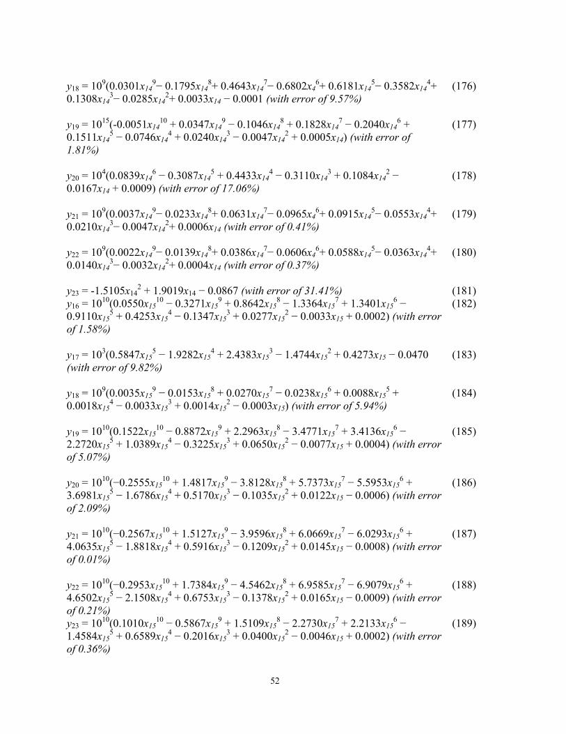
52

y18 = 109(0.0301x14

9− 0.1795x148+ 0.4643x14

7− 0.6802x46+ 0.6181x14

5− 0.3582x144+

0.1308x143− 0.0285x14

2+ 0.0033x14 − 0.0001 (with error of 9.57%)

(176)

y19 = 1015(-0.0051x1410 + 0.0347x14

9 − 0.1046x148 + 0.1828x14

7 − 0.2040x146 +

0.1511x145 − 0.0746x14

4 + 0.0240x143 − 0.0047x14

2 + 0.0005x14) (with error of 1.81%)

(177)

y20 = 104(0.0839x146 − 0.3087x14

5 + 0.4433x144 − 0.3110x14

3 + 0.1084x142 −

0.0167x14 + 0.0009) (with error of 17.06%)

(178)

y21 = 109(0.0037x149− 0.0233x14

8+ 0.0631x147− 0.0965x4

6+ 0.0915x145− 0.0553x14

4+ 0.0210x14

3− 0.0047x142+ 0.0006x14 (with error of 0.41%)

(179)

y22 = 109(0.0022x149− 0.0139x14

8+ 0.0386x147− 0.0606x4

6+ 0.0588x145− 0.0363x14

4+ 0.0140x14

3− 0.0032x142+ 0.0004x14 (with error of 0.37%)

(180)

y23 = -1.5105x142 + 1.9019x14 − 0.0867 (with error of 31.41%) (181)

y16 = 1010(0.0550x1510 − 0.3271x15

9 + 0.8642x158 − 1.3364x15

7 + 1.3401x156 −

0.9110x155 + 0.4253x15

4 − 0.1347x153 + 0.0277x15

2 − 0.0033x15 + 0.0002) (with error of 1.58%)

(182)

y17 = 103(0.5847x155 − 1.9282x15

4 + 2.4383x153 − 1.4744x15

2 + 0.4273x15 − 0.0470 (with error of 9.82%)

(183)

y18 = 109(0.0035x159 − 0.0153x15

8 + 0.0270x157 − 0.0238x15

6 + 0.0088x155 +

0.0018x154 − 0.0033x15

3 + 0.0014x152 − 0.0003x15) (with error of 5.94%)

(184)

y19 = 1010(0.1522x1510 − 0.8872x15

9 + 2.2963x158 − 3.4771x15

7 + 3.4136x156 −

2.2720x155 + 1.0389x15

4 − 0.3225x153 + 0.0650x15

2 − 0.0077x15 + 0.0004) (with error of 5.07%)

(185)

y20 = 1010(−0.2555x1510 + 1.4817x15

9 − 3.8128x158 + 5.7373x15

7 − 5.5953x156 +

3.6981x155 − 1.6786x15

4 + 0.5170x153 − 0.1035x15

2 + 0.0122x15 − 0.0006) (with error of 2.09%)

(186)

y21 = 1010(−0.2567x1510 + 1.5127x15

9 − 3.9596x158 + 6.0669x15

7 − 6.0293x156 +

4.0635x155 − 1.8818x15

4 + 0.5916x153 − 0.1209x15

2 + 0.0145x15 − 0.0008) (with error of 0.01%)

(187)

y22 = 1010(−0.2953x1510 + 1.7384x15

9 − 4.5462x158 + 6.9585x15

7 − 6.9079x156 +

4.6502x155 − 2.1508x15

4 + 0.6753x153 − 0.1378x15

2 + 0.0165x15 − 0.0009) (with error of 0.21%)

(188)

y23 = 1010(0.1010x1510 − 0.5867x15

9 + 1.5109x158 − 2.2730x15

7 + 2.2133x156 −

1.4584x155 + 0.6589x15

4 − 0.2016x153 + 0.0400x15

2 − 0.0046x15 + 0.0002) (with error of 0.36%)

(189)

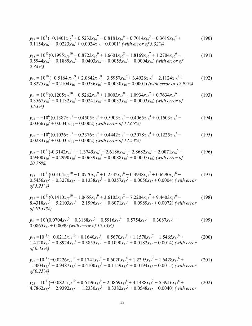
53

y17 = 108 (−0.1401x16

7 + 0.5233x167 − 0.8181x16

6 + 0.7014x165 − 0.3619x16

4 + 0.1154x16

3 − 0.0223x162 + 0.0024x16 − 0.0001) (with error of 3.32%)

(190)

y18 = 1013(0.1995x1610 − 0.8723x16

9 + 1.6601x168 − 1.8169x16

7 + 1.2704x166 −

0.5944x165 + 0.1889x16

4 − 0.0403x163 + 0.0055x16

2 − 0.0004x16) (with error of 2.34%)

(191)

y19 = 1010 (−0.5164 x169 + 2.0842x16

8 − 3.5957x167 + 3.4926x16

6 − 2.1124x165 +

0.8275x164 − 0.2104x16

3 + 0.0336x162 − 0.0030x16

+ 0.0001) (with error of 12.92%)

(192)

y20 = 1013(0.1205x1610 − 0.5262x16

9 + 1.0003x168 − 1.0934x16

7 + 0.7634x166 −

0.3567x165 + 0.1132x16

4 − 0.0241x163 + 0.0033x16

2 − 0.0003x16) (with error of 3.53%)

(193)

y21 = −106 (0.1387x167 − 0.4505x16

6 + 0.5903x165 − 0.4065x16

4 + 0.1603x163 −

0.0366x162 + 0.0045x16 − 0.0002) (with error of 14.65%)

(194)

y22 = −106 (0.1036x167 − 0.3376x16

6 + 0.4442x165 − 0.3078x16

4 + 0.1225x163 −

0.0283x162 + 0.0035x16 − 0.0002) (with error of 12.53%)

(195)

y23 = 1013(-0.3142x1610 + 1.3749x16

9 − 2.6186x168 + 2.8682x16

7 − 2.0071x166 +

0.9400x165 − 0.2990x16

4 + 0.0639x163 − 0.0088x16

2 + 0.0007x16) (with error of 20.76%)

(196)

y18 = 1011(0.0104x1710 − 0.0770x17

9 + 0.2542x178 − 0.4948x17

7 + 0.6290x176 −

0.5456x175 + 0.3270x17

4 − 0.1338x173 + 0.0357x17

2 − 0.0056x17 + 0.0004) (with error of 5.25%)

(197)

y19 = 1011(0.1410x1710 − 1.0658x17

9 + 3.6105x178 − 7.2204x17

7 + 9.4403x176 −

8.4318x175 + 5.2103x17

4 − 2.1996x173 + 0.6071x17

2 − 0.0989x17 + 0.0072) (with error of 10.31%)

(198)

y20 = 105(0.0704x176 − 0.3188x17

5 + 0.5916x174 − 0.5754x17

3 + 0.3087x172 −

0.0865x17 + 0.0099 (with error of 15.13%)

(199)

y21 =1011( −0.0213x1710 + 0.1640x17

9 − 0.5670x178 + 1.1578x17

7 − 1.5465x176 +

1.4120x175 − 0.8924x17

4 + 0.3855x173 − 0.1090x17

2 + 0.0182x17 − 0.0014) (with error of 0.33%)

(200)

y22 =1011( −0.0226x1710 + 0.1741x17

9 − 0.6020x178 + 1.2295x17

7 − 1.6428x176 +

1.5004x175 − 0.9487x17

4 + 0.4100x173 − 0.1159x17

2 + 0.0194x17 − 0.0015) (with error of 0.25%)

(201)

y23 = 1011(−0.0825x1710 + 0.6196x17

9 − 2.0869x178 + 4.1488x17

7 − 5.3916x176 +

4.7862x175 − 2.9392x17

4 + 1.2330x173 − 0.3382x17

2 + 0.0548x17 − 0.0040) (with error (202)

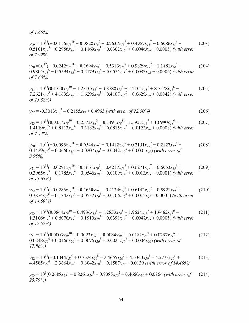
54

of 1.66%) y19 = 1012(−0.0116x18

10 + 0.0828x189 − 0.2637x18

8 + 0.4957x187 − 0.6086x18

6 + 0.5101x18

5 − 0.2956x184 + 0.1169x18

3 − 0.0302x182 + 0.0046x18 − 0.0003) (with error

of 7.92%)

(203)

y20 =1012( −0.0242x1810 + 0.1694x18

9 − 0.5313x188 + 0.9829x18

7 − 1.1881x186 +

0.9805x185 − 0.5594x18

4 + 0.2179x183 − 0.0555x18

2 + 0.0083x18 − 0.0006) (with error of 7.60%)

(204)

y21 = 1012(0.1750x1810 − 1.2310x18

9 + 3.8788x188 − 7.2105x18

7 + 8.7578x186 −

7.2621x185 + 4.1635x18

4 − 1.6296x183 + 0.4167x18

2 − 0.0629x18 + 0.0042) (with error of 25.32%)

(205)

y22 = -0.3013x182 – 0.2155x18 + 0.4963 (with error of 22.50%)

(206)

y23 = 1012(0.0337x1810 − 0.2372x18

9 + 0.7491x188 − 1.3957x18

7 + 1.6990x186 −

1.4119x185 + 0.8113x18

4 − 0.3182x183 + 0.0815x18

2 − 0.0123x18 + 0.0008) (with error of 7.44%)

(207)

y20 = 1012(−0.0093x1910 + 0.0544x19

9 − 0.1412x198 + 0.2151x19

7 − 0.2127x196 +

0.1429x195 − 0.0660x19

4 + 0.0207x193 − 0.0042x19

2 + 0.0005x19) (with error of 3.95%)

(208)

y21 = 1012(−0.0291x1910 + 0.1661x19

9 − 0.4217x198 + 0.6271x19

7 − 0.6053x196 +

0.3965x195 − 0.1785x19

4 + 0.0546x193 − 0.0109x19

2 + 0.0013x19 − 0.0001) (with error of 18.68%)

(209)

y22 = 1012(−0.0286x1910 + 0.1630x19

9 − 0.4134x198 + 0.6142x19

7 − 0.5921x196 +

0.3874x195 − 0.1742x19

4 + 0.0532x193 − 0.0106x19

2 + 0.0012x19 – 0.0001) (with error of 14.59%)

(210)

y23 = 1012(0.0844x1910 − 0.4936x19

9 + 1.2853x198 − 1.9624x19

7 + 1.9462x196 −

1.3106x195 + 0.6070x19

4 − 0.1910x193 + 0.0391x19

2 − 0.0047x19 + 0.0003) (with error of 12.52%)

(211)

y21 = 1015(0.0003x2010 − 0.0023x20

9 + 0.0084x208 − 0.0182x20

7 + 0.0257x206 −

0.0248x205 + 0.0166x20

4 − 0.0076x203 + 0.0023x20

2 − 0.0004x20) (with error of 17.86%)

(212)

y22 = 1010(−0.1044x209 + 0.7624x20

8 − 2.4655x207 + 4.6340x20

6 − 5.5778x205 +

4.4585x204 − 2.3664x20

3 + 0.8042x202 − 0.1587x20 + 0.0139 (with error of 14.46%)

(213)

y23 = 103(0.2688x204 − 0.8261x20

3 + 0.9385x202 − 0.4660x20 + 0.0854 (with error of

23.79%)

(214)

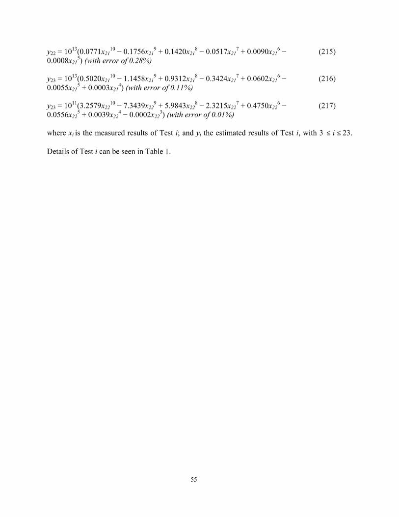
55

y22 = 1013(0.0771x2110 − 0.1756x21

9 + 0.1420x218 − 0.0517x21

7 + 0.0090x216 −

0.0008x215) (with error of 0.28%)

(215)

y23 = 1013(0.5020x2110 − 1.1458x21

9 + 0.9312x218 − 0.3424x21

7 + 0.0602x216 −

0.0055x215 + 0.0003x21

4) (with error of 0.11%)

(216)

y23 = 1011(3.2579x2210 − 7.3439x22

9 + 5.9843x228 − 2.3215x22

7 + 0.4750x226 −

0.0556x225 + 0.0039x22

4 − 0.0002x223) (with error of 0.01%)

(217)

where xi is the measured results of Test i; and yi the estimated results of Test i, with 3 ≤ i ≤ 23.

Details of Test i can be seen in Table 1.

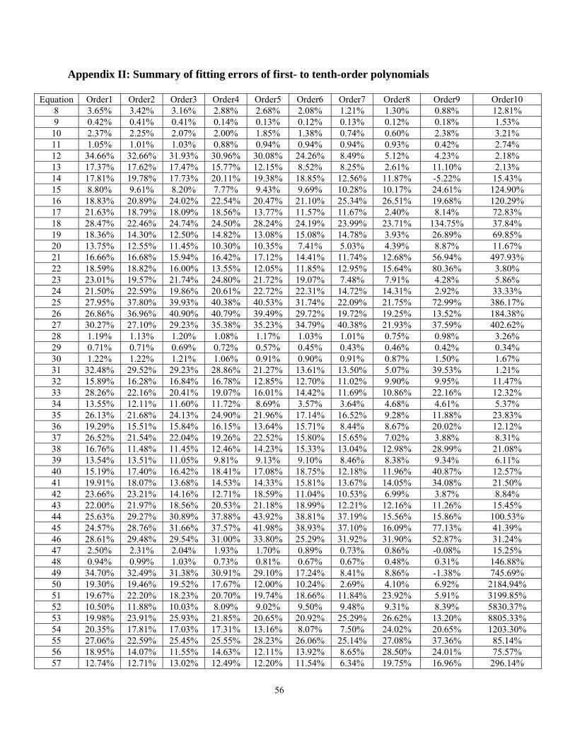
56

Appendix II: Summary of fitting errors of first- to tenth-order polynomials

Equation Order1 Order2 Order3 Order4 Order5 Order6 Order7 Order8 Order9 Order10 8 3.65% 3.42% 3.16% 2.88% 2.68% 2.08% 1.21% 1.30% 0.88% 12.81% 9 0.42% 0.41% 0.41% 0.14% 0.13% 0.12% 0.13% 0.12% 0.18% 1.53%

10 2.37% 2.25% 2.07% 2.00% 1.85% 1.38% 0.74% 0.60% 2.38% 3.21% 11 1.05% 1.01% 1.03% 0.88% 0.94% 0.94% 0.94% 0.93% 0.42% 2.74% 12 34.66% 32.66% 31.93% 30.96% 30.08% 24.26% 8.49% 5.12% 4.23% 2.18% 13 17.37% 17.62% 17.47% 15.77% 12.15% 8.52% 8.25% 2.61% 11.10% 2.13% 14 17.81% 19.78% 17.73% 20.11% 19.38% 18.85% 12.56% 11.87% -5.22% 15.43% 15 8.80% 9.61% 8.20% 7.77% 9.43% 9.69% 10.28% 10.17% 24.61% 124.90% 16 18.83% 20.89% 24.02% 22.54% 20.47% 21.10% 25.34% 26.51% 19.68% 120.29% 17 21.63% 18.79% 18.09% 18.56% 13.77% 11.57% 11.67% 2.40% 8.14% 72.83% 18 28.47% 22.46% 24.74% 24.50% 28.24% 24.19% 23.99% 23.71% 134.75% 37.84% 19 18.36% 14.30% 12.50% 14.82% 13.08% 15.08% 14.78% 3.93% 26.89% 69.85% 20 13.75% 12.55% 11.45% 10.30% 10.35% 7.41% 5.03% 4.39% 8.87% 11.67% 21 16.66% 16.68% 15.94% 16.42% 17.12% 14.41% 11.74% 12.68% 56.94% 497.93% 22 18.59% 18.82% 16.00% 13.55% 12.05% 11.85% 12.95% 15.64% 80.36% 3.80% 23 23.01% 19.57% 21.74% 24.80% 21.72% 19.07% 7.48% 7.91% 4.28% 5.86% 24 21.50% 22.59% 19.86% 20.61% 22.72% 22.31% 14.72% 14.31% 2.92% 33.33% 25 27.95% 37.80% 39.93% 40.38% 40.53% 31.74% 22.09% 21.75% 72.99% 386.17% 26 26.86% 36.96% 40.90% 40.79% 39.49% 29.72% 19.72% 19.25% 13.52% 184.38% 27 30.27% 27.10% 29.23% 35.38% 35.23% 34.79% 40.38% 21.93% 37.59% 402.62% 28 1.19% 1.13% 1.20% 1.08% 1.17% 1.03% 1.01% 0.75% 0.98% 3.26% 29 0.71% 0.71% 0.69% 0.72% 0.57% 0.45% 0.43% 0.46% 0.42% 0.34% 30 1.22% 1.22% 1.21% 1.06% 0.91% 0.90% 0.91% 0.87% 1.50% 1.67% 31 32.48% 29.52% 29.23% 28.86% 21.27% 13.61% 13.50% 5.07% 39.53% 1.21% 32 15.89% 16.28% 16.84% 16.78% 12.85% 12.70% 11.02% 9.90% 9.95% 11.47% 33 28.26% 22.16% 20.41% 19.07% 16.01% 14.42% 11.69% 10.86% 22.16% 12.32% 34 13.55% 12.11% 11.60% 11.72% 8.69% 3.57% 3.64% 4.68% 4.61% 5.37% 35 26.13% 21.68% 24.13% 24.90% 21.96% 17.14% 16.52% 9.28% 11.88% 23.83% 36 19.29% 15.51% 15.84% 16.15% 13.64% 15.71% 8.44% 8.67% 20.02% 12.12% 37 26.52% 21.54% 22.04% 19.26% 22.52% 15.80% 15.65% 7.02% 3.88% 8.31% 38 16.76% 11.48% 11.45% 12.46% 14.23% 15.33% 13.04% 12.98% 28.99% 21.08% 39 13.54% 13.51% 11.05% 9.81% 9.13% 9.10% 8.46% 8.38% 9.34% 6.11% 40 15.19% 17.40% 16.42% 18.41% 17.08% 18.75% 12.18% 11.96% 40.87% 12.57% 41 19.91% 18.07% 13.68% 14.53% 14.33% 15.81% 13.67% 14.05% 34.08% 21.50% 42 23.66% 23.21% 14.16% 12.71% 18.59% 11.04% 10.53% 6.99% 3.87% 8.84% 43 22.00% 21.97% 18.56% 20.53% 21.18% 18.99% 12.21% 12.16% 11.26% 15.45% 44 25.63% 29.27% 30.89% 37.88% 43.92% 38.81% 37.19% 15.56% 15.86% 100.53% 45 24.57% 28.76% 31.66% 37.57% 41.98% 38.93% 37.10% 16.09% 77.13% 41.39% 46 28.61% 29.48% 29.54% 31.00% 33.80% 25.29% 31.92% 31.90% 52.87% 31.24% 47 2.50% 2.31% 2.04% 1.93% 1.70% 0.89% 0.73% 0.86% -0.08% 15.25% 48 0.94% 0.99% 1.03% 0.73% 0.81% 0.67% 0.67% 0.48% 0.31% 146.88% 49 34.70% 32.49% 31.38% 30.91% 29.10% 17.24% 8.41% 8.86% -1.38% 745.69% 50 19.30% 19.46% 19.52% 17.67% 12.00% 10.24% 2.69% 4.10% 6.92% 2184.94% 51 19.67% 22.20% 18.23% 20.70% 19.74% 18.66% 11.84% 23.92% 5.91% 3199.85% 52 10.50% 11.88% 10.03% 8.09% 9.02% 9.50% 9.48% 9.31% 8.39% 5830.37% 53 19.98% 23.91% 25.93% 21.85% 20.65% 20.92% 25.29% 26.62% 13.20% 8805.33% 54 20.35% 17.81% 17.03% 17.31% 13.16% 8.07% 7.50% 24.02% 20.65% 1203.30% 55 27.06% 22.59% 25.45% 25.55% 28.23% 26.06% 25.14% 27.08% 37.36% 85.14% 56 18.95% 14.07% 11.55% 14.63% 12.11% 13.92% 8.65% 28.50% 24.01% 75.57% 57 12.74% 12.71% 13.02% 12.49% 12.20% 11.54% 6.34% 19.75% 16.96% 296.14%

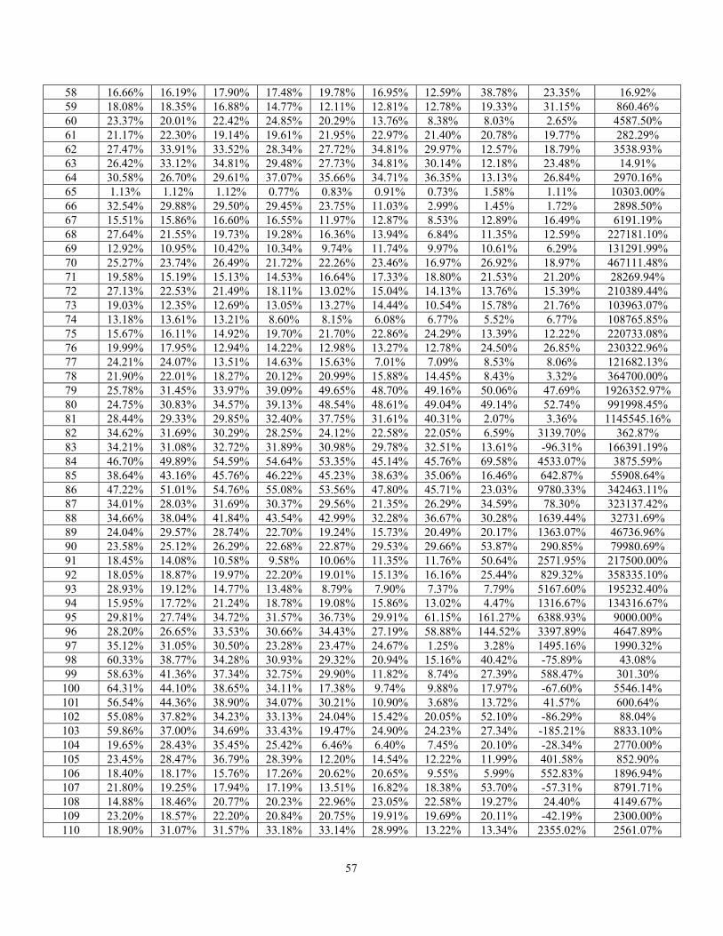
57

58 16.66% 16.19% 17.90% 17.48% 19.78% 16.95% 12.59% 38.78% 23.35% 16.92% 59 18.08% 18.35% 16.88% 14.77% 12.11% 12.81% 12.78% 19.33% 31.15% 860.46% 60 23.37% 20.01% 22.42% 24.85% 20.29% 13.76% 8.38% 8.03% 2.65% 4587.50% 61 21.17% 22.30% 19.14% 19.61% 21.95% 22.97% 21.40% 20.78% 19.77% 282.29% 62 27.47% 33.91% 33.52% 28.34% 27.72% 34.81% 29.97% 12.57% 18.79% 3538.93% 63 26.42% 33.12% 34.81% 29.48% 27.73% 34.81% 30.14% 12.18% 23.48% 14.91% 64 30.58% 26.70% 29.61% 37.07% 35.66% 34.71% 36.35% 13.13% 26.84% 2970.16% 65 1.13% 1.12% 1.12% 0.77% 0.83% 0.91% 0.73% 1.58% 1.11% 10303.00% 66 32.54% 29.88% 29.50% 29.45% 23.75% 11.03% 2.99% 1.45% 1.72% 2898.50% 67 15.51% 15.86% 16.60% 16.55% 11.97% 12.87% 8.53% 12.89% 16.49% 6191.19% 68 27.64% 21.55% 19.73% 19.28% 16.36% 13.94% 6.84% 11.35% 12.59% 227181.10% 69 12.92% 10.95% 10.42% 10.34% 9.74% 11.74% 9.97% 10.61% 6.29% 131291.99% 70 25.27% 23.74% 26.49% 21.72% 22.26% 23.46% 16.97% 26.92% 18.97% 467111.48% 71 19.58% 15.19% 15.13% 14.53% 16.64% 17.33% 18.80% 21.53% 21.20% 28269.94% 72 27.13% 22.53% 21.49% 18.11% 13.02% 15.04% 14.13% 13.76% 15.39% 210389.44% 73 19.03% 12.35% 12.69% 13.05% 13.27% 14.44% 10.54% 15.78% 21.76% 103963.07% 74 13.18% 13.61% 13.21% 8.60% 8.15% 6.08% 6.77% 5.52% 6.77% 108765.85% 75 15.67% 16.11% 14.92% 19.70% 21.70% 22.86% 24.29% 13.39% 12.22% 220733.08% 76 19.99% 17.95% 12.94% 14.22% 12.98% 13.27% 12.78% 24.50% 26.85% 230322.96% 77 24.21% 24.07% 13.51% 14.63% 15.63% 7.01% 7.09% 8.53% 8.06% 121682.13% 78 21.90% 22.01% 18.27% 20.12% 20.99% 15.88% 14.45% 8.43% 3.32% 364700.00% 79 25.78% 31.45% 33.97% 39.09% 49.65% 48.70% 49.16% 50.06% 47.69% 1926352.97% 80 24.75% 30.83% 34.57% 39.13% 48.54% 48.61% 49.04% 49.14% 52.74% 991998.45% 81 28.44% 29.33% 29.85% 32.40% 37.75% 31.61% 40.31% 2.07% 3.36% 1145545.16% 82 34.62% 31.69% 30.29% 28.25% 24.12% 22.58% 22.05% 6.59% 3139.70% 362.87% 83 34.21% 31.08% 32.72% 31.89% 30.98% 29.78% 32.51% 13.61% -96.31% 166391.19% 84 46.70% 49.89% 54.59% 54.64% 53.35% 45.14% 45.76% 69.58% 4533.07% 3875.59% 85 38.64% 43.16% 45.76% 46.22% 45.23% 38.63% 35.06% 16.46% 642.87% 55908.64% 86 47.22% 51.01% 54.76% 55.08% 53.56% 47.80% 45.71% 23.03% 9780.33% 342463.11% 87 34.01% 28.03% 31.69% 30.37% 29.56% 21.35% 26.29% 34.59% 78.30% 323137.42% 88 34.66% 38.04% 41.84% 43.54% 42.99% 32.28% 36.67% 30.28% 1639.44% 32731.69% 89 24.04% 29.57% 28.74% 22.70% 19.24% 15.73% 20.49% 20.17% 1363.07% 46736.96% 90 23.58% 25.12% 26.29% 22.68% 22.87% 29.53% 29.66% 53.87% 290.85% 79980.69% 91 18.45% 14.08% 10.58% 9.58% 10.06% 11.35% 11.76% 50.64% 2571.95% 217500.00% 92 18.05% 18.87% 19.97% 22.20% 19.01% 15.13% 16.16% 25.44% 829.32% 358335.10% 93 28.93% 19.12% 14.77% 13.48% 8.79% 7.90% 7.37% 7.79% 5167.60% 195232.40% 94 15.95% 17.72% 21.24% 18.78% 19.08% 15.86% 13.02% 4.47% 1316.67% 134316.67% 95 29.81% 27.74% 34.72% 31.57% 36.73% 29.91% 61.15% 161.27% 6388.93% 9000.00% 96 28.20% 26.65% 33.53% 30.66% 34.43% 27.19% 58.88% 144.52% 3397.89% 4647.89% 97 35.12% 31.05% 30.50% 23.28% 23.47% 24.67% 1.25% 3.28% 1495.16% 1990.32% 98 60.33% 38.77% 34.28% 30.93% 29.32% 20.94% 15.16% 40.42% -75.89% 43.08% 99 58.63% 41.36% 37.34% 32.75% 29.90% 11.82% 8.74% 27.39% 588.47% 301.30%

100 64.31% 44.10% 38.65% 34.11% 17.38% 9.74% 9.88% 17.97% -67.60% 5546.14% 101 56.54% 44.36% 38.90% 34.07% 30.21% 10.90% 3.68% 13.72% 41.57% 600.64% 102 55.08% 37.82% 34.23% 33.13% 24.04% 15.42% 20.05% 52.10% -86.29% 88.04% 103 59.86% 37.00% 34.69% 33.43% 19.47% 24.90% 24.23% 27.34% -185.21% 8833.10% 104 19.65% 28.43% 35.45% 25.42% 6.46% 6.40% 7.45% 20.10% -28.34% 2770.00% 105 23.45% 28.47% 36.79% 28.39% 12.20% 14.54% 12.22% 11.99% 401.58% 852.90% 106 18.40% 18.17% 15.76% 17.26% 20.62% 20.65% 9.55% 5.99% 552.83% 1896.94% 107 21.80% 19.25% 17.94% 17.19% 13.51% 16.82% 18.38% 53.70% -57.31% 8791.71% 108 14.88% 18.46% 20.77% 20.23% 22.96% 23.05% 22.58% 19.27% 24.40% 4149.67% 109 23.20% 18.57% 22.20% 20.84% 20.75% 19.91% 19.69% 20.11% -42.19% 2300.00% 110 18.90% 31.07% 31.57% 33.18% 33.14% 28.99% 13.22% 13.34% 2355.02% 2561.07%

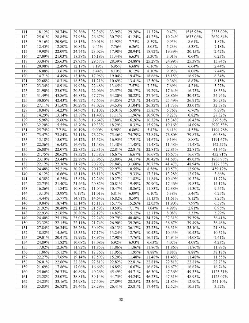
58

111 18.12% 28.74% 29.36% 32.36% 33.95% 29.28% 11.37% 9.47% 1515.98% 2335.09% 112 25.61% 28.85% 27.95% 26.67% 30.75% 41.24% 41.25% 10.24% 1633.06% 2629.84% 113 19.16% 20.96% 18.15% 20.01% 11.92% 7.75% 8.59% 9.95% 8.61% 1.87% 114 12.45% 12.80% 10.84% 9.45% 7.76% 6.36% 5.05% 5.23% 5.38% 7.18% 115 19.98% 22.09% 24.74% 23.02% 17.98% 20.94% 18.92% 19.39% 20.15% 2.42% 116 27.09% 21.03% 18.38% 16.18% 11.44% 6.63% 5.30% 3.01% 0.64% 0.23% 117 33.04% 25.63% 29.93% 29.57% 28.39% 24.88% 25.29% 24.99% 25.38% 15.84% 118 20.98% 12.49% 12.17% 8.19% 6.95% 6.68% 6.16% 6.77% 6.64% 2.44% 119 16.08% 13.61% 18.11% 8.44% 8.19% 8.12% 8.10% 9.05% 8.08% 7.44% 120 14.71% 14.49% 13.16% 17.96% 19.04% 19.47% 18.68% 18.15% 16.97% 6.34% 121 22.68% 18.31% 18.52% 11.21% 10.69% 13.41% 12.50% 9.36% 8.87% 8.15% 122 23.34% 18.91% 19.92% 22.48% 13.45% 7.57% 7.23% 7.69% 4.21% 5.27% 123 21.90% 23.07% 20.54% 22.06% 23.57% 20.17% 19.29% 17.64% 16.73% 18.53% 124 31.49% 43.86% 46.83% 47.77% 34.20% 30.22% 27.76% 28.86% 30.43% 24.94% 125 30.05% 42.43% 46.72% 47.65% 34.85% 27.81% 24.62% 25.49% 26.91% 20.73% 126 27.11% 31.50% 30.29% 43.02% 34.53% 31.04% 26.32% 31.73% 33.01% 32.58% 127 18.04% 14.23% 14.96% 17.10% 15.01% 15.89% 15.85% 6.76% 6.76% 9.89% 128 14.29% 13.14% 13.88% 11.49% 11.11% 11.96% 10.90% 9.22% 0.82% 27.32% 129 15.96% 15.60% 16.36% 16.64% 17.80% 16.26% 16.32% 15.34% 10.43% 279.56% 130 32.20% 15.55% 18.70% 19.33% 18.29% 18.32% 15.92% 19.16% 14.09% 2920.53% 131 25.74% 7.71% 10.19% 9.00% 8.98% 6.86% 5.42% 6.41% 4.53% 1194.78% 132 73.47% 73.84% 74.11% 76.27% 75.46% 74.79% 73.84% 76.80% 79.87% 60.38% 133 15.18% 15.07% 16.12% 15.52% 16.95% 17.91% 14.67% 9.19% 8.88% 1191.67% 134 22.36% 16.45% 16.69% 11.48% 11.48% 11.48% 11.48% 11.48% 11.48% 142.52% 135 26.88% 22.07% 22.83% 22.81% 22.81% 22.81% 22.81% 22.81% 22.81% 41.34% 136 21.75% 20.62% 18.32% 17.38% 16.67% 16.67% 16.67% 16.67% 16.67% 432.81% 137 23.19% 23.44% 22.89% 23.96% 23.89% 34.17% 30.42% 41.68% 49.03% 1863.93% 138 22.12% 22.36% 21.78% 20.29% 21.84% 31.68% 30.73% 41.47% 48.94% 2127.33% 139 24.48% 25.21% 30.20% 20.17% 22.97% 10.55% 8.58% 10.57% 12.90% 459.12% 140 16.12% 16.66% 18.11% 18.11% 18.67% 19.33% 17.21% 13.28% 12.07% 3.86% 141 16.38% 16.25% 15.87% 12.26% 10.27% 11.82% 11.84% 10.49% 10.32% 11.77% 142 22.75% 21.40% 21.46% 20.82% 20.81% 19.49% 20.90% 17.46% 19.83% 14.17% 143 16.26% 11.84% 10.86% 11.04% 10.47% 10.86% 11.83% 12.38% 11.30% 9.54% 144 13.13% 13.98% 9.19% 11.01% 6.81% 6.09% 6.10% 5.38% 5.46% 6.25% 145 14.44% 15.77% 14.71% 14.64% 16.82% 8.59% 11.13% 11.61% 8.12% 8.25% 146 19.04% 18.74% 15.14% 15.11% 15.77% 15.26% 12.03% 11.90% 7.99% 6.57% 147 21.92% 20.48% 22.15% 21.59% 10.59% 7.17% 7.04% 4.99% 2.81% 0.95% 148 22.93% 21.65% 20.80% 22.12% 14.82% 15.12% 12.71% 8.08% 5.33% 5.29% 149 24.40% 25.13% 25.07% 22.24% 29.79% 40.48% 34.37% 37.31% 39.59% 36.41% 150 23.32% 22.15% 22.11% 21.74% 26.90% 39.26% 34.47% 36.67% 39.49% 36.46% 151 27.84% 36.34% 36.26% 30.97% 40.13% 36.17% 37.23% 36.31% 35.10% 21.83% 152 18.52% 14.56% 15.35% 17.17% 13.24% 12.76% 10.43% 10.43% 10.43% 10.52% 153 29.01% 20.41% 19.99% 18.97% 17.98% 17.76% 16.71% 14.94% 14.08% 7.41% 154 24.89% 11.82% 10.08% 13.08% 6.92% 6.93% 6.63% 4.07% 4.09% 4.23% 155 17.02% 12.36% 11.92% 11.85% 11.86% 11.86% 11.86% 11.86% 11.86% 11.99% 156 11.86% 15.12% 10.51% 12.76% 11.95% 11.95% 8.88% 8.88% 8.88% 38.18% 157 22.27% 17.69% 19.14% 17.59% 15.20% 11.48% 11.48% 11.48% 11.48% 11.55% 158 26.01% 22.66% 22.88% 22.81% 22.82% 22.81% 22.81% 22.81% 22.81% 22.73% 159 21.69% 17.86% 17.06% 16.66% 16.85% 16.67% 16.67% 16.67% 16.67% 16.74% 160 25.06% 26.33% 40.89% 40.26% 45.49% 44.71% 46.30% 47.36% 49.33% 1123.31% 161 23.28% 25.07% 38.81% 39.14% 44.75% 44.24% 46.23% 47.31% 48.95% 1125.07% 162 24.23% 33.16% 24.98% 27.50% 27.89% 28.35% 23.46% 21.85% 12.90% 241.10% 163 25.83% 26.82% 29.46% 28.29% 26.41% 25.81% 17.44% 12.52% 10.51% 3.52%

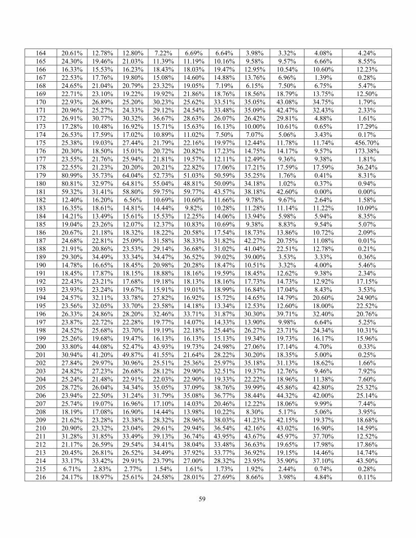
59

164 20.61% 12.78% 12.80% 7.22% 6.69% 6.64% 3.98% 3.32% 4.08% 4.24% 165 24.30% 19.46% 21.03% 11.39% 11.19% 10.16% 9.58% 9.57% 6.66% 8.55% 166 16.33% 15.53% 16.23% 18.43% 18.03% 19.47% 12.95% 10.54% 10.60% 12.23% 167 22.53% 17.76% 19.80% 15.08% 14.60% 14.88% 13.76% 6.96% 1.39% 0.28% 168 24.65% 21.04% 20.79% 23.32% 19.05% 7.19% 6.15% 7.50% 6.75% 5.47% 169 22.71% 23.10% 19.22% 19.92% 21.86% 18.76% 18.56% 18.79% 13.75% 12.50% 170 22.93% 26.89% 25.20% 30.23% 25.62% 33.51% 35.05% 43.08% 34.75% 1.79% 171 20.96% 25.27% 24.33% 29.12% 24.54% 33.48% 35.09% 42.47% 32.43% 2.33% 172 26.91% 30.77% 30.32% 36.67% 28.63% 26.07% 26.42% 29.81% 4.88% 1.61% 173 17.28% 10.48% 16.92% 15.71% 15.63% 16.13% 10.00% 10.61% 0.65% 17.29% 174 26.53% 17.59% 17.02% 10.89% 11.02% 7.50% 7.07% 5.06% 3.43% 0.17% 175 25.38% 19.03% 27.44% 21.79% 22.16% 19.97% 12.44% 11.78% 11.74% 456.70% 176 20.30% 18.50% 15.01% 20.72% 20.82% 17.23% 14.75% 14.17% 9.57% 173.38% 177 23.55% 21.76% 25.94% 21.81% 19.57% 12.11% 12.49% 9.36% 9.38% 1.81% 178 22.55% 21.23% 20.20% 20.21% 22.82% 17.06% 17.21% 17.59% 17.59% 36.24% 179 80.99% 35.73% 64.04% 52.73% 51.03% 50.59% 35.25% 1.76% 0.41% 8.31% 180 80.81% 32.97% 64.81% 55.04% 48.81% 50.09% 34.18% 1.02% 0.37% 0.94% 181 59.32% 31.41% 58.80% 59.75% 59.77% 43.57% 38.18% 42.60% 0.00% 0.00% 182 12.40% 16.20% 6.56% 10.69% 10.60% 11.66% 9.78% 9.67% 2.64% 1.58% 183 16.35% 18.61% 14.81% 14.44% 9.82% 10.28% 11.28% 11.14% 11.22% 10.09% 184 14.21% 13.49% 15.61% 15.53% 12.25% 14.06% 13.94% 5.98% 5.94% 8.35% 185 19.04% 23.26% 12.07% 12.37% 10.83% 10.69% 9.38% 8.83% 9.54% 5.07% 186 20.67% 21.18% 18.32% 18.22% 20.58% 17.54% 18.73% 13.86% 10.72% 2.09% 187 24.68% 22.81% 25.09% 31.58% 38.33% 31.82% 42.27% 20.75% 11.08% 0.01% 188 21.91% 20.86% 23.53% 29.14% 36.68% 31.02% 41.04% 22.51% 12.78% 0.21% 189 29.30% 34.49% 33.34% 34.47% 36.52% 39.02% 39.00% 3.53% 3.33% 0.36% 190 14.78% 16.65% 18.45% 20.98% 20.28% 18.47% 10.51% 3.32% 4.00% 5.46% 191 18.45% 17.87% 18.15% 18.88% 18.16% 19.59% 18.45% 12.62% 9.38% 2.34% 192 22.43% 23.21% 17.68% 19.18% 18.13% 18.16% 17.73% 14.73% 12.92% 17.15% 193 23.93% 23.24% 19.67% 15.91% 19.01% 18.99% 16.84% 17.04% 8.43% 3.53% 194 24.57% 32.11% 33.78% 27.82% 16.92% 15.72% 14.65% 14.79% 20.60% 24.90% 195 23.56% 32.05% 33.70% 23.58% 14.18% 13.34% 12.53% 12.60% 18.00% 22.52% 196 26.33% 24.86% 28.20% 32.46% 33.71% 31.87% 30.30% 39.71% 32.40% 20.76% 197 23.87% 22.72% 22.28% 19.77% 14.07% 14.33% 13.90% 9.98% 6.64% 5.25% 198 24.52% 25.68% 23.70% 19.19% 22.18% 25.44% 26.27% 23.71% 24.34% 10.31% 199 25.26% 19.68% 19.47% 16.13% 16.13% 15.13% 19.34% 19.73% 16.17% 15.96% 200 33.80% 44.08% 52.47% 43.93% 19.73% 24.98% 27.06% 17.14% 4.70% 0.33% 201 30.94% 41.20% 49.87% 41.55% 21.64% 28.22% 30.20% 18.35% 5.00% 0.25% 202 27.84% 29.97% 30.96% 25.51% 25.36% 25.97% 35.18% 31.13% 18.62% 1.66% 203 24.82% 27.23% 26.68% 28.12% 29.90% 32.51% 19.37% 12.76% 9.46% 7.92% 204 25.24% 21.48% 22.91% 22.03% 22.90% 19.33% 22.22% 18.96% 11.38% 7.60% 205 28.72% 26.04% 34.34% 35.05% 37.09% 38.76% 39.99% 45.86% 42.80% 25.32% 206 23.94% 22.50% 31.24% 31.79% 35.08% 36.77% 38.44% 44.32% 42.00% 25.14% 207 25.74% 19.07% 16.96% 17.10% 14.03% 20.46% 12.22% 18.06% 9.99% 7.44% 208 18.19% 17.08% 16.90% 14.44% 13.98% 10.22% 8.30% 5.17% 5.06% 3.95% 209 21.62% 23.28% 23.38% 28.32% 28.96% 38.03% 41.23% 42.15% 19.37% 18.68% 210 20.90% 23.32% 23.04% 29.61% 29.94% 36.54% 42.16% 43.02% 16.90% 14.59% 211 31.28% 31.85% 33.49% 39.13% 36.74% 43.95% 43.67% 45.97% 37.70% 12.52% 212 21.17% 26.59% 29.54% 34.41% 38.04% 33.48% 36.63% 19.65% 17.98% 17.86% 213 20.45% 26.81% 26.52% 34.49% 37.92% 33.77% 36.92% 19.15% 14.46% 14.74% 214 33.17% 33.42% 29.91% 23.79% 27.00% 28.32% 23.95% 35.90% 37.10% 43.50% 215 6.71% 2.83% 2.77% 1.54% 1.61% 1.73% 1.92% 2.44% 0.74% 0.28% 216 24.17% 18.97% 25.61% 24.58% 28.01% 27.69% 8.66% 3.98% 4.84% 0.11%

60

217 23.08% 20.77% 24.06% 23.38% 20.34% 23.86% 20.64% 12.74% 5.37% 6.82E-05

Documents

"Optimal aggregate testing using Vandermonde polynomials and