Embed Size (px)
Citation preview

Technische Universitat MunchenInstitute for Integrated SystemsProf. Dr. sc. techn. Andreas Herkersdorf
Optimal Architecture Synthesis for AircraftElectrical Power Systems
Master Thesis
Author: Safa Messaoud
External advisors: Prof. Alberto Sangiovanni Vincentelli (University of California Berkeley)Advisor: Dr.-Ing. Pierluigi Nuzzo (University of California Berkeley)Supervisor: Prof. Dr. sc. techn. Andreas Herkersdorf
Submission date: June 11, 2013


Contents
Abstract . . . . . . . . . . . . . . . . . . . . . . . . . . . . . . . . . . . . . 2
1 Introduction 3
2 Reliability Analysis Techniques 52.1 Computing Probabilities . . . . . . . . . . . . . . . . . . . . . . . . . 52.2 Numerical Reliability Analysis . . . . . . . . . . . . . . . . . . . . . . 6
2.2.1 Enumeration Methods . . . . . . . . . . . . . . . . . . . . . . 62.2.2 Reliability Block Diagrams . . . . . . . . . . . . . . . . . . . . 72.2.3 Fault Tree Analysis . . . . . . . . . . . . . . . . . . . . . . . . 8
2.3 Symbolic Reliability Analysis . . . . . . . . . . . . . . . . . . . . . . 10
3 Optimal Synthesis of Architectures for Aircraft Electrical Power Systems 153.1 The Aircraft Electrical Power System . . . . . . . . . . . . . . . . . . 15
3.1.1 Components . . . . . . . . . . . . . . . . . . . . . . . . . . . . 153.1.2 System Description . . . . . . . . . . . . . . . . . . . . . . . . 16
3.2 System Specifications . . . . . . . . . . . . . . . . . . . . . . . . . . . 173.2.1 Safety Constraints . . . . . . . . . . . . . . . . . . . . . . . . 173.2.2 Reliability Constraints . . . . . . . . . . . . . . . . . . . . . . 173.2.3 Power Flow Constraints . . . . . . . . . . . . . . . . . . . . . 18
3.3 Design Methodology . . . . . . . . . . . . . . . . . . . . . . . . . . . 183.4 Topology Synthesis Problem Formulation . . . . . . . . . . . . . . . . 18
4 Topology Synthesis Using Mixed Integer Linear Programming ModuloReliability 234.1 Topology Synthesis Flow . . . . . . . . . . . . . . . . . . . . . . . . . 234.2 Mixed Integer Linear Optimizer . . . . . . . . . . . . . . . . . . . . . 24
4.2.1 Power Constraints . . . . . . . . . . . . . . . . . . . . . . . . 254.2.2 Connectivity Constraints . . . . . . . . . . . . . . . . . . . . . 254.2.3 Reliability Constraints . . . . . . . . . . . . . . . . . . . . . . 26
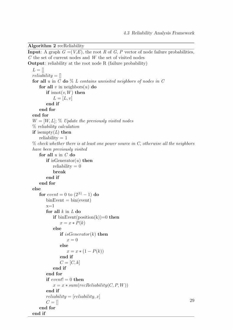
4.3 Reliability Analysis Framework . . . . . . . . . . . . . . . . . . . . . 274.3.1 Recursive Algorithm . . . . . . . . . . . . . . . . . . . . . . . 284.3.2 Iterative Algorithm . . . . . . . . . . . . . . . . . . . . . . . . 31
4.4 Strategies to Increase the Reliability . . . . . . . . . . . . . . . . . . 364.4.1 Moves . . . . . . . . . . . . . . . . . . . . . . . . . . . . . . . 364.4.2 Strategies . . . . . . . . . . . . . . . . . . . . . . . . . . . . . 41
iii
Contents
4.5 Handling Contactors . . . . . . . . . . . . . . . . . . . . . . . . . . . 424.5.1 Generating Switch Connectivity Matrices . . . . . . . . . . . . 424.5.2 Extending the Adjacency Matrix . . . . . . . . . . . . . . . . 44
4.6 Soundness and Completeness . . . . . . . . . . . . . . . . . . . . . . . 464.7 Synthesis Results . . . . . . . . . . . . . . . . . . . . . . . . . . . . . 47
4.7.1 Strategy 1 . . . . . . . . . . . . . . . . . . . . . . . . . . . . . 494.7.2 Strategy 2 . . . . . . . . . . . . . . . . . . . . . . . . . . . . . 544.7.3 Comparison . . . . . . . . . . . . . . . . . . . . . . . . . . . . 56
5 Topology Synthesis Using Plain Mixed Integer Linear Programming 595.1 Plain MILP with Exact Reliability Algebra . . . . . . . . . . . . . . . 60
5.1.1 Synthesis of the Reliability Expression . . . . . . . . . . . . . 605.1.2 Linearization of the Reliability Expression . . . . . . . . . . . 615.1.3 Synthesis Flow Example . . . . . . . . . . . . . . . . . . . . . 635.1.4 Results and Challenges . . . . . . . . . . . . . . . . . . . . . . 69
5.2 Plain MILP with Approximate Reliability Algebra . . . . . . . . . . . 705.2.1 Approximation Technique . . . . . . . . . . . . . . . . . . . . 705.2.2 Example of Approximate Reliability Constraint Generation . . 725.2.3 Synthesis Results . . . . . . . . . . . . . . . . . . . . . . . . . 74
5.3 Comparison Between MILP Modulo Reliability and Plain MILP . . . 75
6 Conclusions and Future Work 77
iv
List of Tables
4.1 Power capability of the generators [W] (Template 1) . . . . . . . . . . 474.2 Power requirements of the loads [W] (Template 1) . . . . . . . . . . . 484.3 Power capability of the generators [W] (Template 2) . . . . . . . . . . 484.4 Power requirements of the loads [W] (Template 2) . . . . . . . . . . . 484.5 Costs of the components . . . . . . . . . . . . . . . . . . . . . . . . . 484.6 Failure probability of the components . . . . . . . . . . . . . . . . . . 484.7 Reliability at the loads (Strategy 1, Template 1, non failing switches) 494.8 Reliability at the loads (Strategy 1, Template 1, failing switches) . . 494.9 Reliability at the loads (Strategy 1, Template 2, non failing switches) 524.10 Reliability at the loads (Strategy 2, Template 1, non failing switches) 544.11 Reliability at the loads (Strategy 2, Template 2, non failing switches) 564.12 Reliability at the loads (Strategy 2, Template 1, failing switches) . . . 564.13 Comparison between strategy 1 and strategy 2 . . . . . . . . . . . . . 56
5.1 Results of the Plain MILP with exact reliability algebra . . . . . . . . 695.2 Results of the Plain MILP with approximate reliability algebra (Tem-
plate 2) . . . . . . . . . . . . . . . . . . . . . . . . . . . . . . . . . . 745.3 Comparison between Plain MILP and MILP Modulo Reliability . . . 76
v

List of Figures
2.1 Reliability analysis using the state enumeration method [1] . . . . . . 7
2.2 Example of a Reliability Block Diagram . . . . . . . . . . . . . . . . 8
2.3 A hydraulic system [2] . . . . . . . . . . . . . . . . . . . . . . . . . . 9
2.4 Fault Tree Analysis of the hydraulic system in Figure 2.3 [2] . . . . . 10
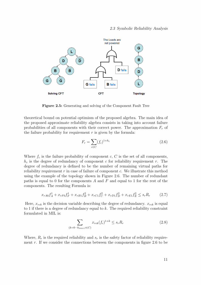
2.5 Generating and solving of the Component Fault Tree . . . . . . . . . 11
2.6 Example of the Reliability synthesis using approximate reliability al-gebra . . . . . . . . . . . . . . . . . . . . . . . . . . . . . . . . . . . . 12
3.1 Single Line Diagram of an electrical power system adapted from aHoneywell Patent [3] . . . . . . . . . . . . . . . . . . . . . . . . . . . 16
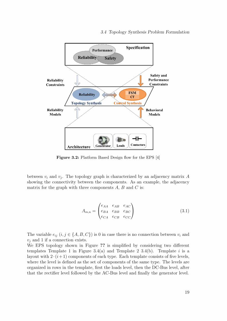
3.2 Platform Based Design flow for the EPS [4] . . . . . . . . . . . . . . . 19
3.3 Platform Based Design for EPS topology synthesis . . . . . . . . . . . 20
3.4 Templates of the EPS topology . . . . . . . . . . . . . . . . . . . . . 20
4.1 Flow of the MILP Modulo Reliability approach . . . . . . . . . . . . 23
4.2 Simple topology . . . . . . . . . . . . . . . . . . . . . . . . . . . . . . 27
4.3 Recursive reliability algorithm demonstration . . . . . . . . . . . . . 30
4.4 Iterative Reliability Algoritm . . . . . . . . . . . . . . . . . . . . . . 34
4.5 Iterative reliability algorithm demonstration . . . . . . . . . . . . . . 35
4.6 Move 1 . . . . . . . . . . . . . . . . . . . . . . . . . . . . . . . . . . . 36
4.7 Move 3 . . . . . . . . . . . . . . . . . . . . . . . . . . . . . . . . . . . 38
4.8 Move 6 . . . . . . . . . . . . . . . . . . . . . . . . . . . . . . . . . . . 39
4.9 Move 7 . . . . . . . . . . . . . . . . . . . . . . . . . . . . . . . . . . . 40
4.10 Move 9 . . . . . . . . . . . . . . . . . . . . . . . . . . . . . . . . . . . 41
4.11 Induction proof for soundness and completness . . . . . . . . . . . . . 47
4.12 Topologies resulting from Strategy 1 (Template 1, non failing switches) 50
4.13 Topologies resulting from Strategy 1 (Template 2, non failing switches) 51
4.14 Topologies resulting from Strategy 1 (Template 2, non failing switches) 52
4.15 Topologies resulting from Strategy 1 (Template 1, failing switches) . . 53
4.16 Topologies resulting from Strategy 2 (Template 1, non failing switches) 54
4.17 Topologies resulting from Strategy 2 (Template 2, non failing switches) 55
4.18 Topologies resulting from Strategy 2 (Template 1, failing switches) . . 55
5.1 Topology Synthesis Flow (Plain MILP) . . . . . . . . . . . . . . . . . 60
vii
List of Figures
5.2 Topology used to illustrate the symbolic synthesis of reliability ex-pressions . . . . . . . . . . . . . . . . . . . . . . . . . . . . . . . . . . 61
5.3 Example of the synthesis and linearization of the reliability constraints 635.4 Example illustrating the Plain MILP with exact reliability algebra
approach (Iterations 1-15) . . . . . . . . . . . . . . . . . . . . . . . . 685.5 Example illustrating the Plain MILP with exact reliability algebra
approach (Iterations 16-25) . . . . . . . . . . . . . . . . . . . . . . . . 695.6 Plain MILP with exact reliability algebra generated topologies . . . . 705.7 Components’ insertion rules . . . . . . . . . . . . . . . . . . . . . . . 715.8 Plain MILP with approximate reliability algebra (Template 1) . . . . 745.9 Plain MILP with approximate reliability algebra (Template 2) . . . . 75
viii
List of Figures
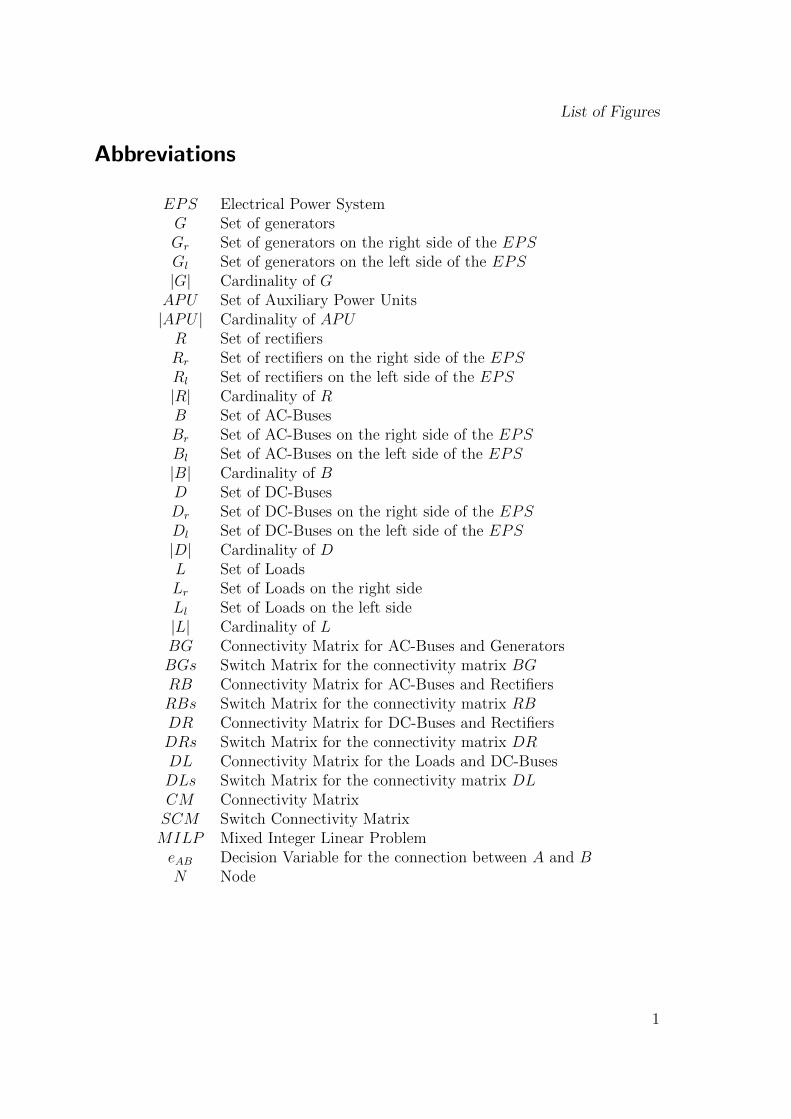
Abbreviations
EPS Electrical Power SystemG Set of generatorsGr Set of generators on the right side of the EPSGl Set of generators on the left side of the EPS|G| Cardinality of GAPU Set of Auxiliary Power Units|APU | Cardinality of APUR Set of rectifiersRr Set of rectifiers on the right side of the EPSRl Set of rectifiers on the left side of the EPS|R| Cardinality of RB Set of AC-BusesBr Set of AC-Buses on the right side of the EPSBl Set of AC-Buses on the left side of the EPS|B| Cardinality of BD Set of DC-BusesDr Set of DC-Buses on the right side of the EPSDl Set of DC-Buses on the left side of the EPS|D| Cardinality of DL Set of LoadsLr Set of Loads on the right sideLl Set of Loads on the left side|L| Cardinality of LBG Connectivity Matrix for AC-Buses and GeneratorsBGs Switch Matrix for the connectivity matrix BGRB Connectivity Matrix for AC-Buses and RectifiersRBs Switch Matrix for the connectivity matrix RBDR Connectivity Matrix for DC-Buses and RectifiersDRs Switch Matrix for the connectivity matrix DRDL Connectivity Matrix for the Loads and DC-BusesDLs Switch Matrix for the connectivity matrix DLCM Connectivity MatrixSCM Switch Connectivity MatrixMILP Mixed Integer Linear ProblemeAB Decision Variable for the connection between A and BN Node
1

List of Figures
Abstract
Aircraft Electrical Power Systems (EPS) are becoming complex cyber-physical sys-tems, consisting of a physical plant (generators, AC-Buses, rectifiers, DC-Buses,switches and loads) and a cyber component, namely the Bus Power Control Units(BPCU).To deal with the increasing complexity of EPS while guaranteeing the satisfactionof tight reliability and safety constraints, automated design tools for the synthesis ofthe topology (interconnection of components) are developed. These tools can signif-icantly reduce the design time aiming to generate correct-by-construction systems.In this thesis, we propose two optimization oriented design methodologies to syn-thesize a reliable-by-construction EPS topology with minimal cost and complexity.The two methodologies differently deal with the non linear reliability constraint,that arise in the mathematical formulation of the synthesis problem.The first methodology uses a Mixed Integer Linear Programming Modulo Reliability(MILPMR) approach to generate minimal cost topologies, given a set of a connec-tivity and power flow constraints. The optimizer is placed in a loop with a reliabilityanalysis algorithm, which evaluates the failure probability of the critical loads andimplements several strategies that provide suggestions to the optimizer to improvethe reliability of the topology, in case the requirements are not met.In the second methodology, we automatically generate a symbolic expression of thereliability analysis, linearize it and use it directly in a plain MILP optimizer.We successfully implement the two methodologies and compare them with respectto their runtime, scalability with the number of components and accuracy.The obtained results show that the MILPMR can result in a less efficient implemen-tation because of the number of iterations needed to converge to the final solution,whereas the plain MILP normally converges in one iterations, but it relies on anapproximate reliability algebra to improve on scalability.
2
1 Introduction
The fast development in power electronics and embedded processors has allowed anincreasing electrification of embedded systems during the last decade [5]. The vehicleindustry has moved from using conventional pneumatic, mechanical and hydrauliccomponents to implementing cyber physical ones. This has certainly led to an in-creasing overall power efficiency. However, the rising complexity of such systems ispresenting a major challenge for the designers. These systems consist of numerousphysical and cyber interconnected components that share resources and interact insafety critical ways under performance, real-time and reliability constraints. As aresult, the traditional heuristic design methods and processes, mainly based on theskills of the designer and the previous experience tend to become ineffective andpossibly yield to long redesign cycles, costs and delays.
A similar challenge was met by the integrated circuits industry some decades ago,and has been efficiently solved by raising the level of abstraction [6]. Automateddesign Automation (ADE) tools has led to breakthroughs in the IC-Design market.They significantly helped to manage the exponential increase in the capability toimplement integrated circuits that incorporate billions of transistors. They have alsosuccessfully combined different theories in computation and modeling. A similar ap-proach is now being advocated for system-level design of cyber physical systems [7].Automated design tools will enable designers to work at a higher level of abstrac-tion and to algorithmically synthesize Cyber Physical systems which are correct byconstruction.
This thesis deals with developing an automated synthesis tool for the architecture ofan aircraft electrical power system. The contribution of this work consists of intro-ducing two different methodologies to automatically synthesize reliable by construc-tion EPS architectures, where an architecture is defined as a set of interconnectedcomponents. Given a set of reliability, power flow and performance constraints, amixed integer linear optimizer synthesizes a minimal cost and complexity topology.Since the reliability constraints are non linear, we use two approaches to deal withthem in the optimization process.
In a first approach, which we call Mixed Integer Linear Programming modulo Re-liability (MILP Modulo Reliability), we place a reliability analysis tool in a loopwith an optimizer. The optimizer first synthesizes a solution from the power flow
3
1 Introduction
and performance constraints. The reliability of the obtained topology is determinedusing the reliability analysis tool. If the required reliability is reached, a valid topol-ogy is returned, otherwise, different strategies are used to add more connectivityconstraints to original formulation of the problem. The new constraints force moreredundancy in paths or components in order to increase the reliability. This processis repeated until a valid solution, i.e a reliable architecture, is reached.
The second approach consists of linearizing a symbolic reliability expression andusing it directly in a Plain MILP optimizer. For this purpose, we first synthesizethe reliability expression for a reconfigurable topology considering the connectionsbetween the components as the decision variables. Then, we use linearization tech-niques to derive mixed integer linear constraints out of the synthesized reliabilityexpression. We first try an exact reliability algebra for the synthesis of the reliabil-ity expression. However, this method poorly scales with the number of components.Thus, we opt for an approximate reliability algebra that generates a reliability ex-pression based on the redundancy of the components.
The thesis is organized as follow: Chapter 2 is a survey of different methods toanalyze the reliability of an architecture. In Chapter 3, we give a brief descriptionof an airplane electrical power system, state the problem formulation and presentthe used design methodologies and models. Chapter 4 and 5 deal with the synthesisof topologies, using, respectively the MILP Modulo Reliability and the Plain MILPapproaches. We also compare these two methodologies with respect to their scala-bility with the number of components, efficiency and accuracy. We close this thesiswith some concluding remarks and suggested future work.
4
2 Reliability Analysis Techniques
The reliability of a system is defined as its ability to perform its required functionsunder stated conditions for a specified period of time. System reliability is one ofthe biggest challenge of system engineering. Different tools and methods have beendeveloped to assess the system reliability in the early design phases to prevent fore-seeable problems and minimize the risk of the unforeseen ones. In this chapter, wewill first give an overview on the probability expression generation techniques. Then,we investigate methods for numerical and symbolic reliability analysis. Finally, weshow how the generated expressions can be used in Mixed Integer Linear Problems.
2.1 Computing Probabilities
We are interested in probability expressions that determine how an event failuredepends on other basic events. For example, the expression
F = (A ∪B) ∩ (C ∪D) (2.1)
says that an event F occurs if either A or B and either A or C occur. A, B and C aresubsets of a set S representing all possible outcomes of an experiment. Let P(·) bea probability function defined on the space S. Then, P(A), P(B) and P(C) are theprobabilities that, respectively, the events A, B and C occur. We wish to computeP (F ) = P ((A ∪ B) ∩ (C ∪ D)). We assume that we know the probabilities of thebasic events A, B and C. In the absence of any other information, computing P(F)is generally impossible. Let’s suppose, that events A, B and C are independent inthe probabilistic sense. Thus, P (A ∩ B) = P (A) · P (B). Moreover, (A ∪ B) and(C ∪D) are independent. The formula below results for P(F):
P (F ) = P (F1) · P (F2)
F1 = A ∪BF2 = C ∪D
5
2 Reliability Analysis Techniques
where
P (F1) = P (A ∪B)
= 1− P (A ∩ B)
= 1− (1− P (A)) · (1− P (B))
= P (A) + P (B)− P (A) · P (B)
P (F2) = P (C ∪D)
= P (C) + P (D)− P (C) · P (D)
(2.2)
The analytical formula for P (F ) is then:
P (F ) = (P (A) + P (B)− P (A) · P (B)) · (P (C) + P (D)− P (C) · P (D)) (2.3)
By performing computations such as the ones above, we obtain an analytical formulafor P (F ). This formula depends on the probabilities of basic events. Differentmethods and algorithm have been developed to automatically generate expressionsfor P (F ) .
2.2 Numerical Reliability Analysis
The goal of the numerical reliability analysis methods is, given a system architectureand functionality, to derive the system reliability. Different techniques can be usedfor this purpose. We will first explain the enumeration method that computes thedesired probability value by enumerating all the possible paths or system states.Then, we will present how the reliability can be derived using graphical methodslike the reliability graph and the Fault Tree Analysis.
2.2.1 Enumeration Methods
The enumeration methods are used on a network modeled as a graph. We distinguishbetween the enumeration of states and the enumeration of paths and cuts.
State Enumeration
We consider a network for which the reliability is to be determined. The network ismodeled as a graph G = (V,E) where the nodes V represents the set of componentsand the edges E the set of interconnection between the components. The compo-nents are considered to fail independently of one another with known probabilities.For each component, there are two states: either the component functions or fails.Thus, there are 2|V |+|E| states of the network. The reliability is equal to the sumof the probabilities of the states that lead the system to fail, in case of disjunct
6
2.2 Numerical Reliability Analysis
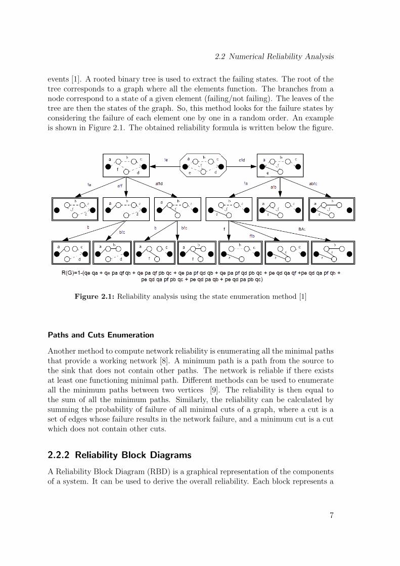
events [1]. A rooted binary tree is used to extract the failing states. The root of thetree corresponds to a graph where all the elements function. The branches from anode correspond to a state of a given element (failing/not failing). The leaves of thetree are then the states of the graph. So, this method looks for the failure states byconsidering the failure of each element one by one in a random order. An exampleis shown in Figure 2.1. The obtained reliability formula is written below the figure.
Figure 2.1: Reliability analysis using the state enumeration method [1]
Paths and Cuts Enumeration
Another method to compute network reliability is enumerating all the minimal pathsthat provide a working network [8]. A minimum path is a path from the source tothe sink that does not contain other paths. The network is reliable if there existsat least one functioning minimal path. Different methods can be used to enumerateall the minimum paths between two vertices [9]. The reliability is then equal tothe sum of all the minimum paths. Similarly, the reliability can be calculated bysumming the probability of failure of all minimal cuts of a graph, where a cut is aset of edges whose failure results in the network failure, and a minimum cut is a cutwhich does not contain other cuts.
2.2.2 Reliability Block Diagrams
A Reliability Block Diagram (RBD) is a graphical representation of the componentsof a system. It can be used to derive the overall reliability. Each block represents a
7
2 Reliability Analysis Techniques
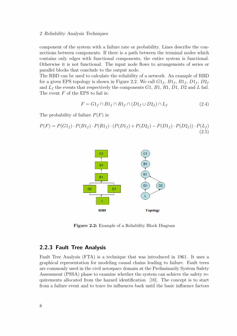
component of the system with a failure rate or probability. Lines describe the con-nections between components. If there is a path between the terminal nodes whichcontains only edges with functional components, the entire system is functional.Otherwise it is not functional. The input node flows to arrangements of series orparallel blocks that conclude to the output node.The RBD can be used to calculate the reliability of a network. An example of RBDfor a given EPS topology is shown in Figure 2.2. We call G1f , B1f , R1f , D1f , D2fand Lf the events that respectively the components G1, B1, R1, D1, D2 and L fail.The event F of the EPS to fail is:
F = G1f ∩B1f ∩R1f ∩ (D1f ∪D2f ) ∩ Lf (2.4)
The probability of failure P (F ) is:
P (F ) = P (G1f ) ·P (B1f ) ·P (R1f ) · (P (D1f ) +P (D2f )−P (D1f ) ·P (D2f )) ·P (Lf )(2.5)
Figure 2.2: Example of a Reliability Block Diagram
2.2.3 Fault Tree Analysis
Fault Tree Analysis (FTA) is a technique that was introduced in 1961. It uses agraphical representation for modeling causal chains leading to failure. Fault treesare commonly used in the civil aerospace domain at the Preliminarily System SafetyAssessment (PSSA) phase to examine whether the system can achieve the safety re-quirements allocated from the hazard identification [10]. The concept is to startfrom a failure event and to trace its influences back until the basic influence factors
8
2.2 Numerical Reliability Analysis
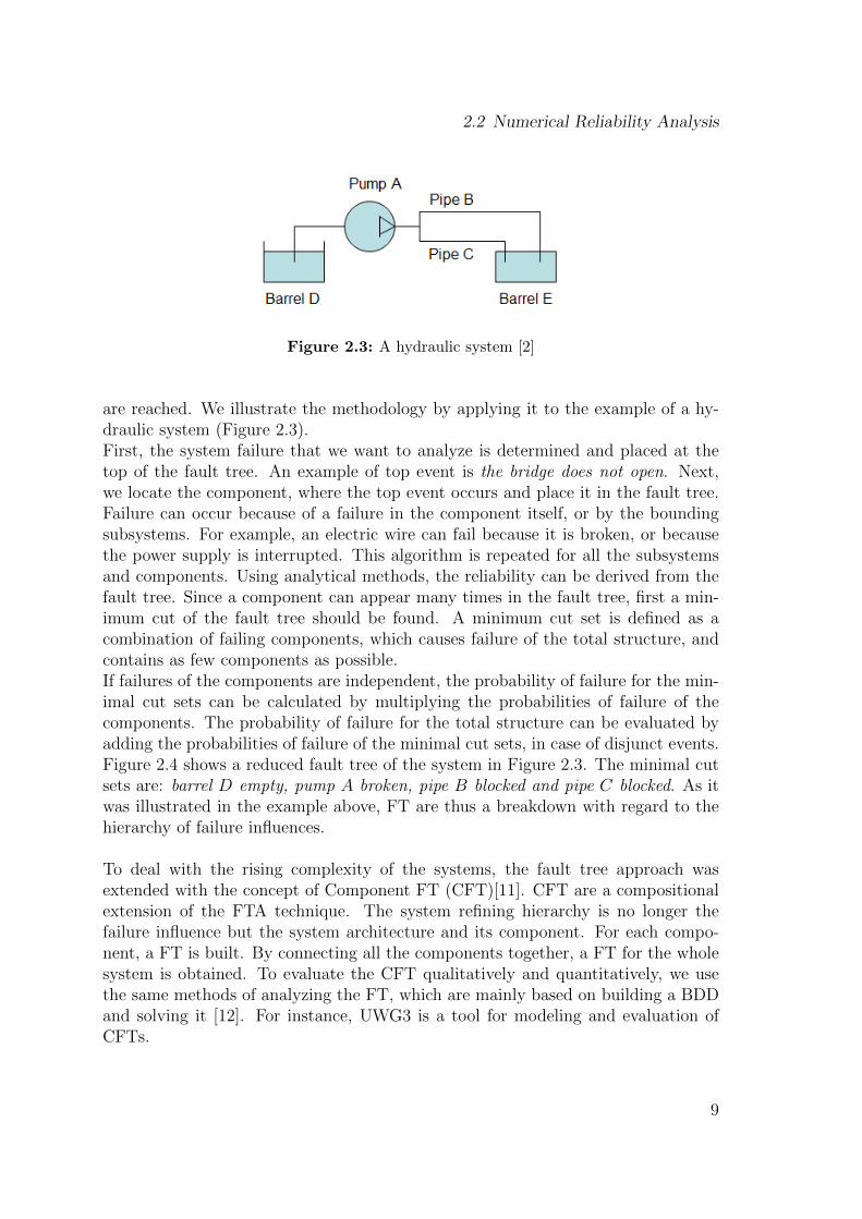
Figure 2.3: A hydraulic system [2]
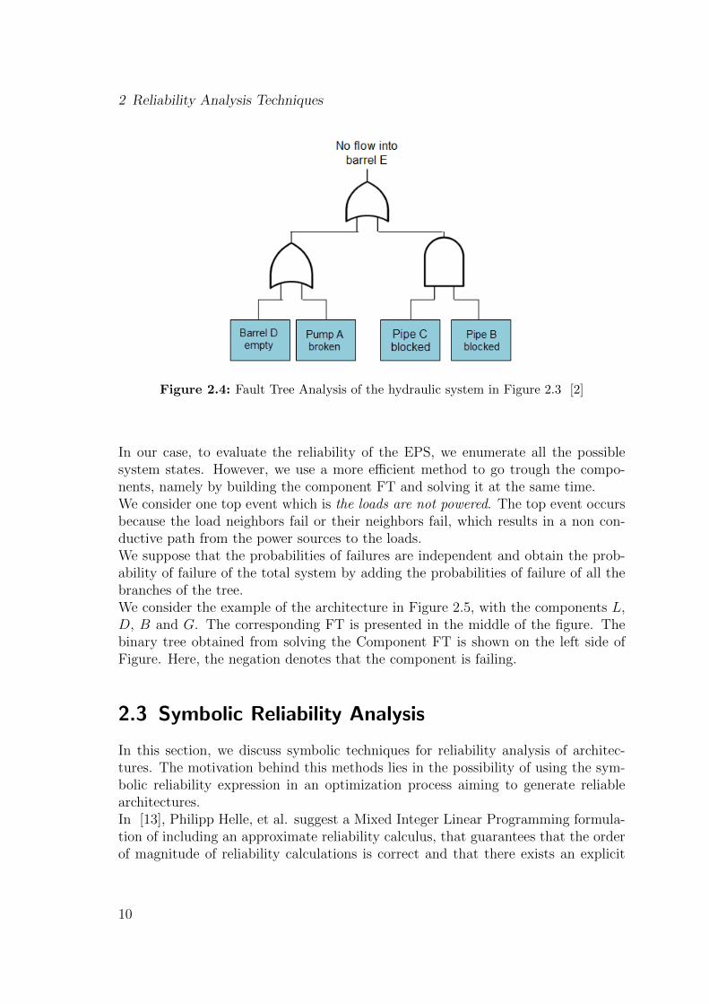
are reached. We illustrate the methodology by applying it to the example of a hy-draulic system (Figure 2.3).First, the system failure that we want to analyze is determined and placed at thetop of the fault tree. An example of top event is the bridge does not open. Next,we locate the component, where the top event occurs and place it in the fault tree.Failure can occur because of a failure in the component itself, or by the boundingsubsystems. For example, an electric wire can fail because it is broken, or becausethe power supply is interrupted. This algorithm is repeated for all the subsystemsand components. Using analytical methods, the reliability can be derived from thefault tree. Since a component can appear many times in the fault tree, first a min-imum cut of the fault tree should be found. A minimum cut set is defined as acombination of failing components, which causes failure of the total structure, andcontains as few components as possible.If failures of the components are independent, the probability of failure for the min-imal cut sets can be calculated by multiplying the probabilities of failure of thecomponents. The probability of failure for the total structure can be evaluated byadding the probabilities of failure of the minimal cut sets, in case of disjunct events.Figure 2.4 shows a reduced fault tree of the system in Figure 2.3. The minimal cutsets are: barrel D empty, pump A broken, pipe B blocked and pipe C blocked. As itwas illustrated in the example above, FT are thus a breakdown with regard to thehierarchy of failure influences.
To deal with the rising complexity of the systems, the fault tree approach wasextended with the concept of Component FT (CFT)[11]. CFT are a compositionalextension of the FTA technique. The system refining hierarchy is no longer thefailure influence but the system architecture and its component. For each compo-nent, a FT is built. By connecting all the components together, a FT for the wholesystem is obtained. To evaluate the CFT qualitatively and quantitatively, we usethe same methods of analyzing the FT, which are mainly based on building a BDDand solving it [12]. For instance, UWG3 is a tool for modeling and evaluation ofCFTs.
9
2 Reliability Analysis Techniques
Figure 2.4: Fault Tree Analysis of the hydraulic system in Figure 2.3 [2]
In our case, to evaluate the reliability of the EPS, we enumerate all the possiblesystem states. However, we use a more efficient method to go trough the compo-nents, namely by building the component FT and solving it at the same time.We consider one top event which is the loads are not powered. The top event occursbecause the load neighbors fail or their neighbors fail, which results in a non con-ductive path from the power sources to the loads.We suppose that the probabilities of failures are independent and obtain the prob-ability of failure of the total system by adding the probabilities of failure of all thebranches of the tree.We consider the example of the architecture in Figure 2.5, with the components L,D, B and G. The corresponding FT is presented in the middle of the figure. Thebinary tree obtained from solving the Component FT is shown on the left side ofFigure. Here, the negation denotes that the component is failing.
2.3 Symbolic Reliability Analysis
In this section, we discuss symbolic techniques for reliability analysis of architec-tures. The motivation behind this methods lies in the possibility of using the sym-bolic reliability expression in an optimization process aiming to generate reliablearchitectures.In [13], Philipp Helle, et al. suggest a Mixed Integer Linear Programming formula-tion of including an approximate reliability calculus, that guarantees that the orderof magnitude of reliability calculations is correct and that there exists an explicit
10
2.3 Symbolic Reliability Analysis
Figure 2.5: Generating and solving of the Component Fault Tree
theoretical bound on potential optimism of the proposed algebra. The main idea ofthe proposed approximate reliability algebra consists in taking into account failureprobabilities of all components with their correct power. The approximation Fr ofthe failure probability for requirement r is given by the formula:
Fr =∑c∈C
(fc)1+hc (2.6)
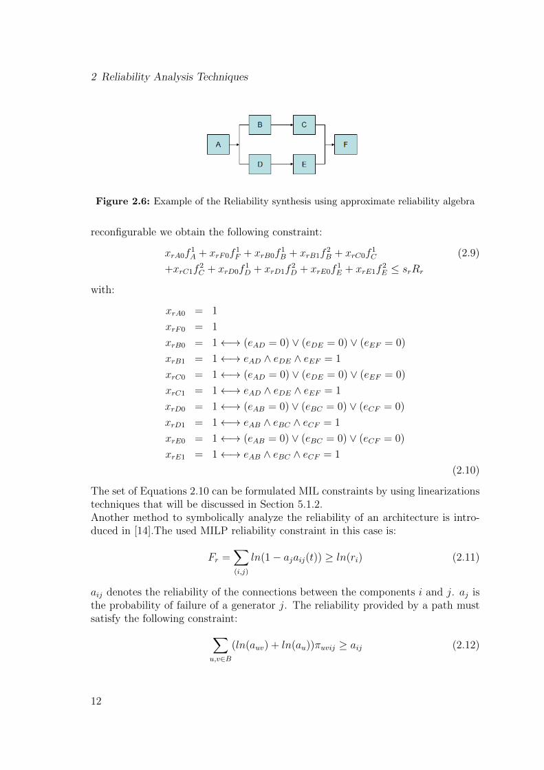
Where fc is the failure probability of component c, C is the set of all components,hc is the degree of redundancy of component c for reliability requirement r. Thedegree of redundancy is defined to be the number of remaining virtual paths forreliability requirement r in case of failure of component c. We illustrate this methodusing the example of the topology shown in Figure 2.6. The number of redundantpaths is equal to 0 for the components A and F and equal to 1 for the rest of thecomponents. The resulting Formula is:
xrA0f1A + xrF0f
1F + xrB1f
2B + xrC1f
2C + xrD1f
2D + xrE1f
2E ≤ srRr (2.7)
Here, xrck is the decision variable describing the degree of redundancy. xrck is equalto 1 if there is a degree of redundancy equal to k. The required reliability constraintformulated in MIL is: ∑
(k=0···kmax,c∈C)
xrck(fc)1+k ≤ srRr (2.8)
Where, Rr is the required reliability and sr is the safety factor of reliability require-ment r. If we consider the connections between the components in figure 2.6 to be
11
2 Reliability Analysis Techniques
Figure 2.6: Example of the Reliability synthesis using approximate reliability algebra
reconfigurable we obtain the following constraint:
xrA0f1A + xrF0f
1F + xrB0f
1B + xrB1f
2B + xrC0f
1C (2.9)
+xrC1f2C + xrD0f
1D + xrD1f
2D + xrE0f
1E + xrE1f
2E ≤ srRr
with:
xrA0 = 1
xrF0 = 1
xrB0 = 1←→ (eAD = 0) ∨ (eDE = 0) ∨ (eEF = 0)
xrB1 = 1←→ eAD ∧ eDE ∧ eEF = 1
xrC0 = 1←→ (eAD = 0) ∨ (eDE = 0) ∨ (eEF = 0)
xrC1 = 1←→ eAD ∧ eDE ∧ eEF = 1
xrD0 = 1←→ (eAB = 0) ∨ (eBC = 0) ∨ (eCF = 0)
xrD1 = 1←→ eAB ∧ eBC ∧ eCF = 1
xrE0 = 1←→ (eAB = 0) ∨ (eBC = 0) ∨ (eCF = 0)
xrE1 = 1←→ eAB ∧ eBC ∧ eCF = 1
(2.10)
The set of Equations 2.10 can be formulated MIL constraints by using linearizationstechniques that will be discussed in Section 5.1.2.Another method to symbolically analyze the reliability of an architecture is intro-duced in [14].The used MILP reliability constraint in this case is:
Fr =∑(i,j)
ln(1− ajaij(t)) ≥ ln(ri) (2.11)
aij denotes the reliability of the connections between the components i and j. aj isthe probability of failure of a generator j. The reliability provided by a path mustsatisfy the following constraint:∑
u,v∈B
(ln(auv) + ln(au))πuvij ≥ aij (2.12)
12

2.3 Symbolic Reliability Analysis
where auv is the reliability of a connector (e.g. a TRU, power converter, contactor),B the set of buses, au is the reliability of a bus and πuvij is a binary variable equalto 1 if the path from i to j uses the connection from u to v. The paper states alimitation of this approach, namely that all paths can not be active at the sametime. It also does not show any implementations of the proposed approach.
In this thesis, we develop an algorithm that evaluates the reliability of a given archi-tecture modeled as a graph by enumerating all the system states in a compositionalway, based on the actual structure of the topology. This is equivalent to building afault tree on the fly and computing the desired probability value or expression. Thisalgorithm is used in a MILP Modulo Reliability approach (as discussed in Chapter4) to check whether a generated topology satisfies the required reliability. Finally,we synthesize symbolic reliability expressions trying both exact and approximatereliability algebras and show how they can be used in a MILP optimization problemin chapter 5.
13


3 Optimal Synthesis of Architecturesfor Aircraft Electrical PowerSystems
In this chapter, we will first give an overview of the aircraft electrical power system.Then, we will go through the main models and design methodology used in thethesis. Finally, we will present a formalization of the topology design problem.
3.1 The Aircraft Electrical Power System
An electric power system for a passenger aircraft comprises generators, APUs, AC-Buses, DC-Buses, rectifiers, contactors and loads, which compose the platform li-brary.
3.1.1 Components
AC generators: AC generators are connected to AC-Buses and generate variablefrequency power.
APU: when one of the generators fails, an APU or an external battery is used toprovide short-term high-integrity power to the AC buses while alternative sourcesare brought online.
AC and DC power buses: AC and DC power buses deliver power to a numberof loads or power conversion equipment. Essential Buses are connected to criticalloads (loads that should always be powered).
Rectifier units: rectifier units are used to convert three-phase AC power to DCpower. Transformers are used to step down high voltages to lower voltages. Acombined transformer rectifier unit both converts power from AC to DC as well aslowers the voltage.
Loads: electrically-driven loads include sub-systems such as lighting, heating, mo-tors and actuation. Some loads are critical and cannot be shed, while others can
15
3 Optimal Synthesis of Architectures for Aircraft Electrical Power Systems
be taken off-line in case of emergency. Loads include, in addition to motors andactuators lighting, heating and cabin pressurization.
Contactors: contactors are high-power switches that control the flow of powerand establish connections between components. Contactors are configured to beopen or closed by the Bus Power Control Units (BPCU), i.e the EPS controllers.
3.1.2 System Description
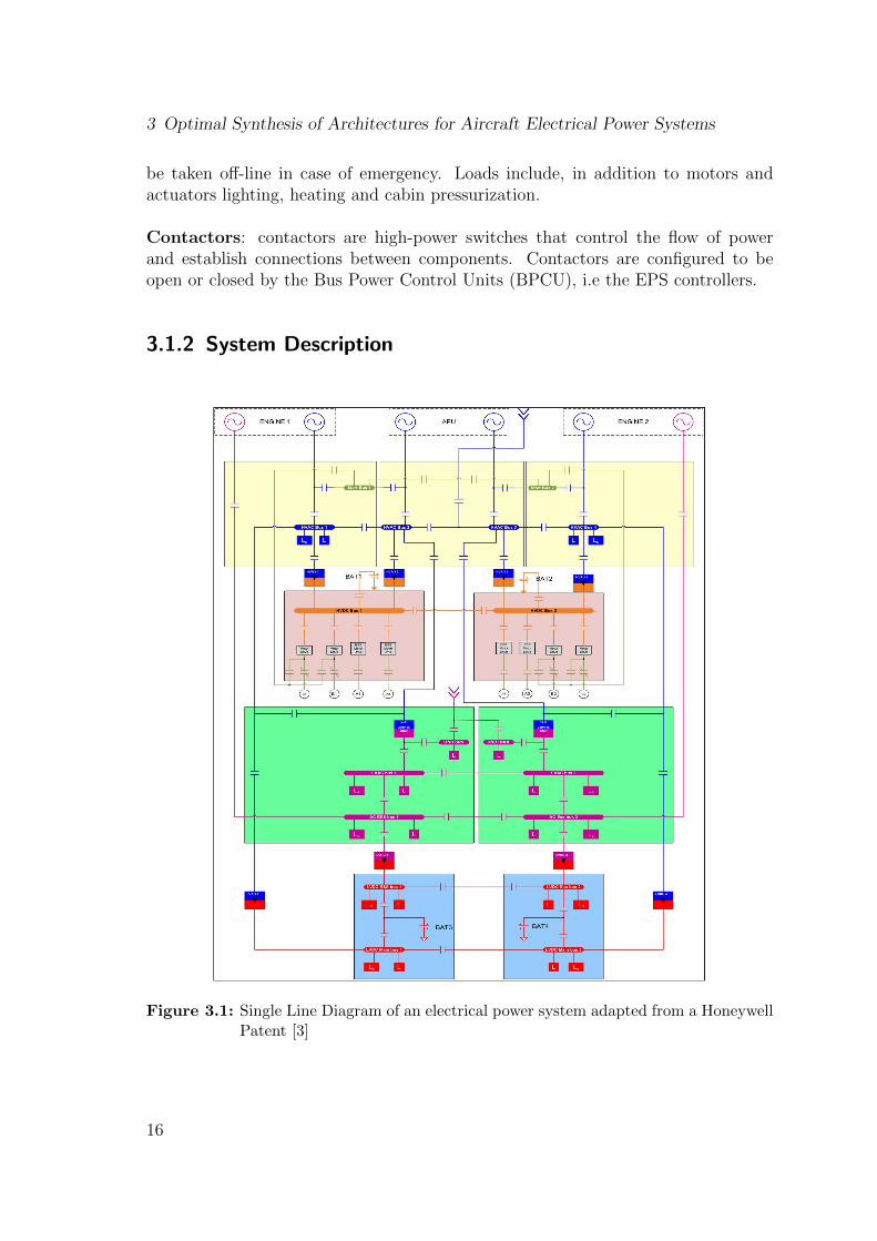
Figure 3.1: Single Line Diagram of an electrical power system adapted from a HoneywellPatent [3]
16
3.2 System Specifications
Figure 3.1 shows a sample architecture for the electric power generation and dis-tribution system in an aircraft. The plant includes six generators and an externalpower source, as it is shown in the top of the diagram. Each engine contains a HighVoltage AC (HVAC) generator (blue) and a Low Voltage AC (LVAC) emergencygenerator (purple). Two high voltage APUs are used as back up power sources.Each HVAC generator/APU is connected to its respective HVAC distribution panelvia contactors (represented by double bars in the single-line diagram). Each panelcontains its own start bus and one or two HVAC buses. The start bus can drawpower from the motor drive to power on either the main generator or the APU.Once the generator is online, the start bus is disconnected. The HVAC Buses 1and 4 are connected to two types of loads: essential loads (L) must remain alwayspowered while sheddable loads (Ls) can be dropped if power supply is insufficient.The four rectifier units RUs are selectively connected to the four HVAC buses onthe one side and to the HVDC Bus on the other side. Each HVDC Bus is alsoselectively connected to a battery and powers a set of motor drives. HVAC Buses 2and 3 are also connected to a set of transformers that convert HVAC to LVAC. TheLow Voltage AC system is contained in the green boxes in the diagram. An externalground source can be applied to the buses for ground services and handling, e.g.operations that are only used when the aircraft is on the ground.
3.2 System Specifications
The requirements of the power system are expressed in terms of reliability, safetyand performance constraints. Examples of each type of these constraints are listedbelow.
3.2.1 Safety Constraints
• To avoid paralleling of AC sources, no AC bus can be powered by multiplegenerators at any point of time
• Total load must be within the capacity of the generators
• Each generator shall be controlled by only one controller
3.2.2 Reliability Constraints
The system must be designed for a failure probability smaller than 10−9. Theprobability of failure is equal to the probability of the system to be unpowered.That is, the systems must be capable of tolerating any combination of componentfaults that has a joint probability more than 10−9.
17

3 Optimal Synthesis of Architectures for Aircraft Electrical Power Systems
3.2.3 Power Flow Constraints
• Power is always first allocated to the non-sheddable loads and then to thesheddable loads by respecting, in all cases, the load priorities
• The electric power system shall provide electric power, so that the AC voltagelevel is between 115 and 120 V and the DC voltage level is 28 V
• Each bus has a priority list by which it can be determined which active gen-erator should be selected to power it
3.3 Design Methodology
A Platform Based Design (PBD) methodology is proposed to design the aircraftelectrical power system in [7], as also shown in Figure 3.3. PBD is defined as a meetin the middle process, where successive refinements of specifications meet with ab-stractions of potential implementations in a common semantic domain. This methodaims to generate a correct-by-construction design. It also allows a structured designspace exploration.The design specifications, expressed in terms of safety, reliability and performanceconstraints are successively refined and meet with abstractions of potential imple-mentations based on the models of the elements of the platform. The platformis defined as a library of components (generators, rectifiers, AC-Buses, DC-Buses,loads). Each component is characterized by a probability of failure, a cost and aset connectivity rules. Loads and generators are also characterized, respectively, bytheir power requirements and power capability. The safety specifications are mostlyunder the responsibility of the control protocol, while the reliability specificationsare mostly under the responsibility of the topology as it is shown in Figure 3.2.We apply the PBD methodology to the design of the topology as shown in Figure3.2. In this case, the functional specifications are the reliability and power flow ones.The platform is a set of components characterized by their failure probabilities andconnectivity rules. We define the common semantic domain to be the optimizationspace where the MILP is formulated. The reliability and power flow specificationsare refined into mixed integer constraints, the platform components are abstractedinto failure models and connectivity constraints. In the common semantic domain,we undertake an optimization process aiming at generating a reliable topology witha minimum cost and complexity from the MIL constraints.
3.4 Topology Synthesis Problem Formulation
The topology is presented by a graph G = (V,E), where each node vi ∈ V representsa component i (i ∈ {1, · · · , n}) and each edge eij ∈ E represents the interconnection
18
3.4 Topology Synthesis Problem Formulation
Figure 3.2: Platform Based Design flow for the EPS [4]
between vi and vj. The topology graph is characterized by an adjacency matrix Ashowing the connectivity between the components. As an example, the adjacencymatrix for the graph with three components A, B and C is:
Am,n =
eAA eAB eACeBA eBB eBCeCA eCB eCC
(3.1)
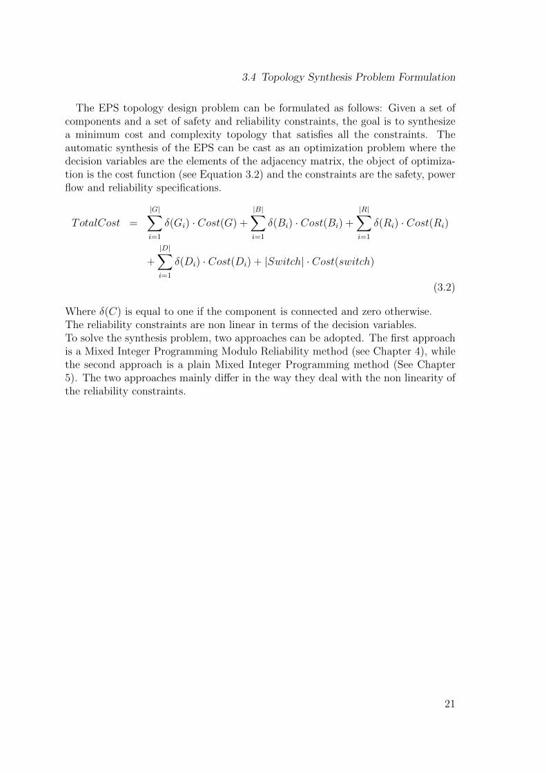
The variable eij (i, j ∈ {A,B,C}) is 0 in case there is no connection between vi andvj and 1 if a connection exists.We EPS topology shown in Figure ?? is simplified by considering two differenttemplates Template 1 in Figure 3.4(a) and Template 2 3.4(b). Template i is alayout with 2 · (i+1) components of each type. Each template consists of five levels,where the level is defined as the set of components of the same type. The levels areorganized in rows in the template, first the loads level, then the DC-Bus level, afterthat the rectifier level followed by the AC-Bus level and finally the generator level.
19
3 Optimal Synthesis of Architectures for Aircraft Electrical Power Systems
Figure 3.3: Platform Based Design for EPS topology synthesis
RG1 RG2
RB1 RB2
RR1 RR2
RD1 RD2
RL1 RL2
APU1LG1 LG2
LB1 LB2
LR1 LR2
LD1 LD2
LL1 LL2
(a) Template 1
RG1 RG2 RG3
RB1 RB2 RB3
RR1 RR2 RR3
RD1 RD2 RD3
RL1 RL2 RL3
APU1LG1 LG2 LG3
LB1 LB2 LB3
LR1 LR2 LR3
LD1 LD2 LD3
LL1 LL2 LL3
(b) Template 2
Figure 3.4: Templates of the EPS topology
20
3.4 Topology Synthesis Problem Formulation
The EPS topology design problem can be formulated as follows: Given a set ofcomponents and a set of safety and reliability constraints, the goal is to synthesizea minimum cost and complexity topology that satisfies all the constraints. Theautomatic synthesis of the EPS can be cast as an optimization problem where thedecision variables are the elements of the adjacency matrix, the object of optimiza-tion is the cost function (see Equation 3.2) and the constraints are the safety, powerflow and reliability specifications.
TotalCost =
|G|∑i=1
δ(Gi) · Cost(G) +
|B|∑i=1
δ(Bi) · Cost(Bi) +
|R|∑i=1
δ(Ri) · Cost(Ri)
+
|D|∑i=1
δ(Di) · Cost(Di) + |Switch| · Cost(switch)
(3.2)
Where δ(C) is equal to one if the component is connected and zero otherwise.The reliability constraints are non linear in terms of the decision variables.To solve the synthesis problem, two approaches can be adopted. The first approachis a Mixed Integer Programming Modulo Reliability method (see Chapter 4), whilethe second approach is a plain Mixed Integer Programming method (See Chapter5). The two approaches mainly differ in the way they deal with the non linearity ofthe reliability constraints.
21

4 Topology Synthesis Using MixedInteger Linear ProgrammingModulo Reliability
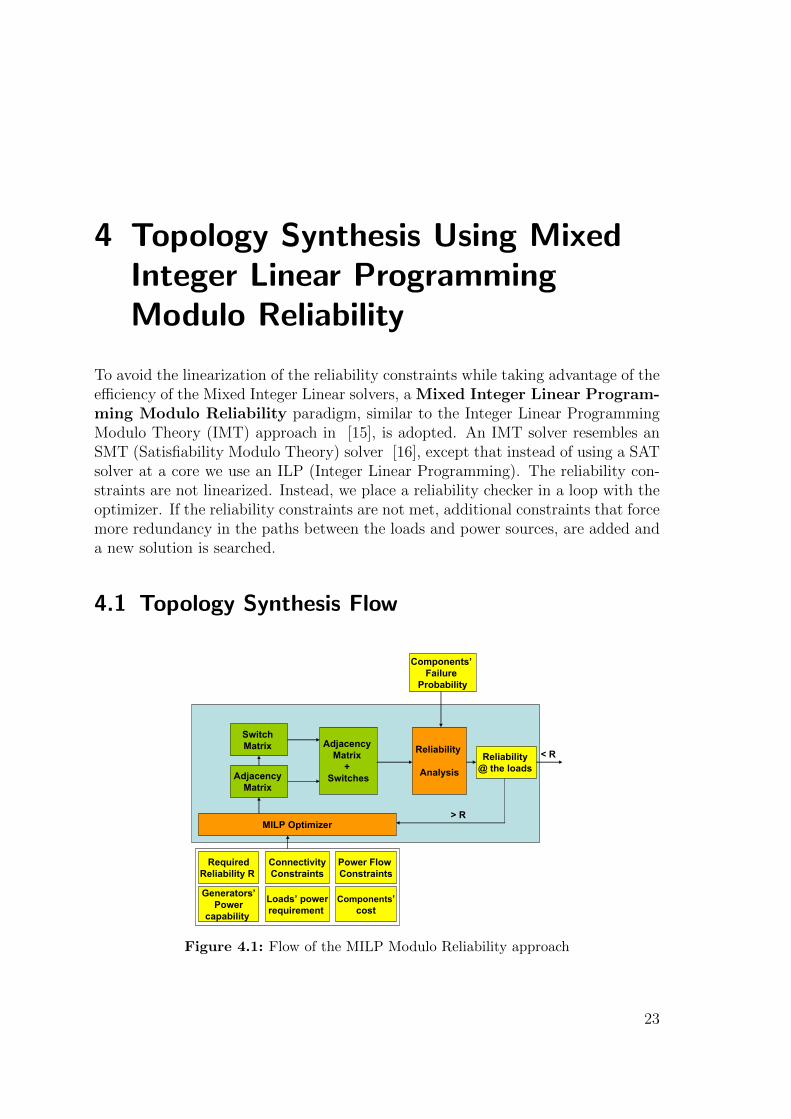
To avoid the linearization of the reliability constraints while taking advantage of theefficiency of the Mixed Integer Linear solvers, a Mixed Integer Linear Program-ming Modulo Reliability paradigm, similar to the Integer Linear ProgrammingModulo Theory (IMT) approach in [15], is adopted. An IMT solver resembles anSMT (Satisfiability Modulo Theory) solver [16], except that instead of using a SATsolver at a core we use an ILP (Integer Linear Programming). The reliability con-straints are not linearized. Instead, we place a reliability checker in a loop with theoptimizer. If the reliability constraints are not met, additional constraints that forcemore redundancy in the paths between the loads and power sources, are added anda new solution is searched.
4.1 Topology Synthesis Flow
MILPCOptimizer
ReliabilityC
Analysis
AdjacencyCMatrixC
+CSwitchesAdjacencyC
MatrixC
SwitchCMatrixC
ReliabilityC@CtheCloadsC
Components’FailureC
Probability
PowerCFlowCConstraints
ConnectivityConstraints
Generators’Power
capabilityC
RequiredReliabilityCRC
Loads’ powerrequirementC
Components’cost
<CR
>CR
Figure 4.1: Flow of the MILP Modulo Reliability approach
23
4 Topology Synthesis Using Mixed Integer Linear Programming Modulo Reliability
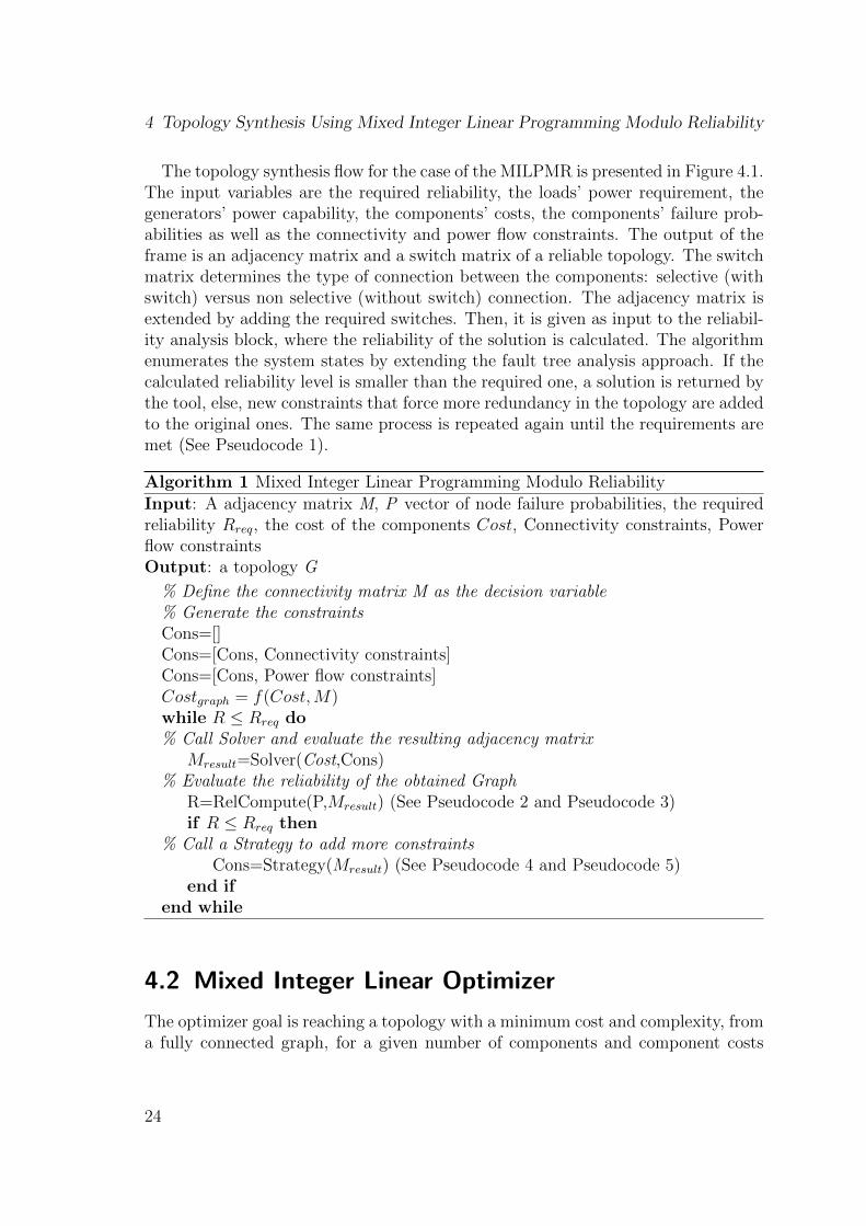
The topology synthesis flow for the case of the MILPMR is presented in Figure 4.1.The input variables are the required reliability, the loads’ power requirement, thegenerators’ power capability, the components’ costs, the components’ failure prob-abilities as well as the connectivity and power flow constraints. The output of theframe is an adjacency matrix and a switch matrix of a reliable topology. The switchmatrix determines the type of connection between the components: selective (withswitch) versus non selective (without switch) connection. The adjacency matrix isextended by adding the required switches. Then, it is given as input to the reliabil-ity analysis block, where the reliability of the solution is calculated. The algorithmenumerates the system states by extending the fault tree analysis approach. If thecalculated reliability level is smaller than the required one, a solution is returned bythe tool, else, new constraints that force more redundancy in the topology are addedto the original ones. The same process is repeated again until the requirements aremet (See Pseudocode 1).
Algorithm 1 Mixed Integer Linear Programming Modulo Reliability
Input: A adjacency matrix M, P vector of node failure probabilities, the requiredreliability Rreq, the cost of the components Cost, Connectivity constraints, Powerflow constraintsOutput: a topology G
% Define the connectivity matrix M as the decision variable% Generate the constraintsCons=[]Cons=[Cons, Connectivity constraints]Cons=[Cons, Power flow constraints]Costgraph = f(Cost,M)while R ≤ Rreq do% Call Solver and evaluate the resulting adjacency matrix
Mresult=Solver(Cost,Cons)% Evaluate the reliability of the obtained Graph
R=RelCompute(P,Mresult) (See Pseudocode 2 and Pseudocode 3)if R ≤ Rreq then
% Call a Strategy to add more constraintsCons=Strategy(Mresult) (See Pseudocode 4 and Pseudocode 5)
end ifend while
4.2 Mixed Integer Linear Optimizer
The optimizer goal is reaching a topology with a minimum cost and complexity, froma fully connected graph, for a given number of components and component costs
24
4.2 Mixed Integer Linear Optimizer
while still satisfying the connectivity and power constraints. In this paragraph, wepresent some examples for the mathematical formulation of the constraints.
4.2.1 Power Constraints
• The sum of the power capability of generators on a one side of the topologytemplate must be greater than or equal to the total requirement of the loadson that side. This holds in normal conditions.
|G|∑i=1
[Power(Gi)(
|B|∨j=1
eGiBj)] ≥
|L|∑h=1
Power(Lh) (4.1)
(Gi ∈ G, i ≤ |G|, Bj ∈ B, j ≤ |B|, Lh ∈ L, h ≤ |L|)Expressed in MILP, Equation 4.1 is equivalent to:
|G|∑i=1
Power(Gi) · maxk≤|B|
(eGiB)k ≥|L|∑h=1
Power(Lh) (4.2)
(Gi ∈ G, i ≤ |G|, Lh ∈ L, h ≤ |L|)
eGiB is the vector of the connections between Gi and the AC-Buses B.
4.2.2 Connectivity Constraints
• A DC-Bus connected to a load or another DC-Bus must be connected to aRectifier
(
|L|∨j=1
eDiLj) ∨(
|D|∨k=1
eDiDk)=
|R|∨h=1
eRhDi(4.3)
(∀Di,k ∈ D with i 6= k, {i, k} ≤ |D|,∀Lj ∈ L, j ≤ |L|, ∀Rh ∈ R, h ≤ |R|)
Expressed in MILP, Equation 4.3 is equivalent to:
max(maxk≤|L|
(eDiL)k, maxh≤|D|
(eDiD)k) = maxr≤|R|
(eRDi)r (4.4)
(∀Di ∈ D)
eDiL is the vector of connections between Di and L. eDiD is the vector of con-nections between Di and the DC-Buses different from Di. eRDi
is the vectorof connections between Di and the rectifiers R.
25

4 Topology Synthesis Using Mixed Integer Linear Programming Modulo Reliability
• AC Buses not connected to a rectifier should not be connected to anotherAC-Bus
|R|∨j=1
eBiRj≥|B|∨k=1
eBiBk(4.5)
(∀Bi,k ∈ B with i 6= k,∀Rj ∈ R, j ≤ |R|)
Expressed in MILP, Equation 4.5 is equivalent to:
maxk≤|R|
(eBiR)k ≥ maxj≤|B|
(eBiB)j (4.6)
(∀Bi ∈ B)
eBiR is the vector of connection between Bi and R. eBiB is the vector of con-nection between Bi and the AC-Buses different from Bi.
• Rectifier cannot be connected to more than one DC Bus.
|D|∑j=1
eRjDi≤ 1 (4.7)
(∀Rj ∈ R, j ≤ |R|,∀Di ∈ D, i ≤ |D|)
• No AC-Bus on one side of the EPS can be connected to itself
eBiBi= 0 (4.8)
(∀Bi ∈ B, i ≤ |B|)
• APU cannot be connected to more than one AC-Bus per side
|B|∑j=1
eAPUiBj=1 (4.9)
(∀Bj ∈ B, j ≤ |B|,∀APUi ∈ APU, i ≤ |APU |)
4.2.3 Reliability Constraints
The reliability constraints describe the bound on probability of failure within thesystem. We define by failure, the situation where the loads are not powered. Everycomponent comes with a reliability level. A level ε of reliability, for example, indi-cates that one failure occurs every 1
εhours.
Given multiple component failures, the system should be designed to tolerate any
26
4.3 Reliability Analysis Framework
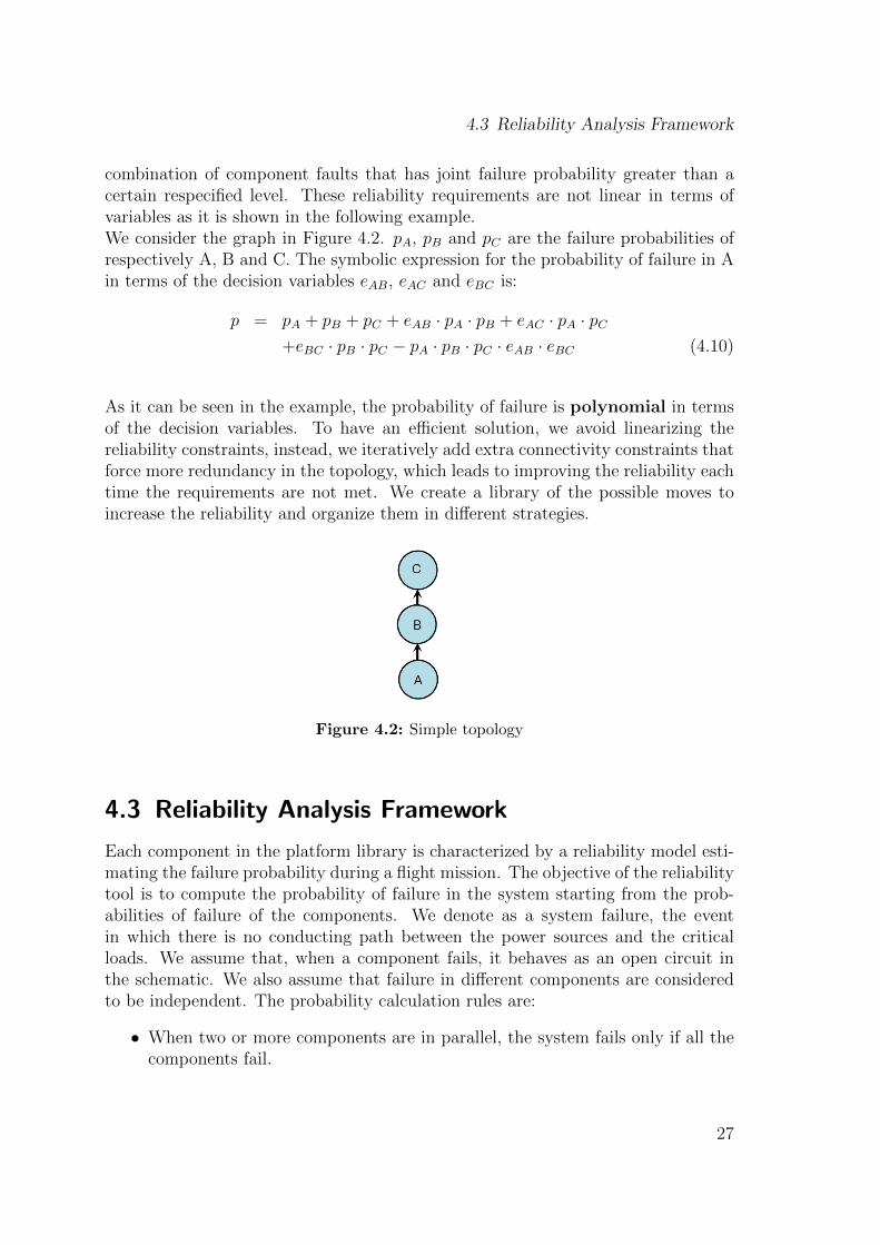
combination of component faults that has joint failure probability greater than acertain respecified level. These reliability requirements are not linear in terms ofvariables as it is shown in the following example.We consider the graph in Figure 4.2. pA, pB and pC are the failure probabilities ofrespectively A, B and C. The symbolic expression for the probability of failure in Ain terms of the decision variables eAB, eAC and eBC is:
p = pA + pB + pC + eAB · pA · pB + eAC · pA · pC+eBC · pB · pC − pA · pB · pC · eAB · eBC (4.10)
As it can be seen in the example, the probability of failure is polynomial in termsof the decision variables. To have an efficient solution, we avoid linearizing thereliability constraints, instead, we iteratively add extra connectivity constraints thatforce more redundancy in the topology, which leads to improving the reliability eachtime the requirements are not met. We create a library of the possible moves toincrease the reliability and organize them in different strategies.
Figure 4.2: Simple topology
4.3 Reliability Analysis Framework
Each component in the platform library is characterized by a reliability model esti-mating the failure probability during a flight mission. The objective of the reliabilitytool is to compute the probability of failure in the system starting from the prob-abilities of failure of the components. We denote as a system failure, the eventin which there is no conducting path between the power sources and the criticalloads. We assume that, when a component fails, it behaves as an open circuit inthe schematic. We also assume that failure in different components are consideredto be independent. The probability calculation rules are:
• When two or more components are in parallel, the system fails only if all thecomponents fail.
27
4 Topology Synthesis Using Mixed Integer Linear Programming Modulo Reliability
• When two or more components are in series, the system fails if at least one ofthe components fails.
In the following, we illustrate two implementations of the reliability computationalgorithm: a recursive implementation which is more intuitive, and an iterative one,which is more efficient.
4.3.1 Recursive Algorithm
The recursive algorithm traverses the graph G from the critical load (root) to thegenerators (leaves) and uses formula 4.11 to represent the system failure event as afunction of failures of other components. We call Pi is the event that component ifails and pi the probability of Pi. The event Fi of a system failure at a component iis given by:
Fi = Pi⋃
j∈[1..K]
Fj (4.11)
where K in the number of neighboring components not previously visited of thecomponent i.In case of a directed tree, the probability of failure at a node i is:
P (Fi) = pi + (1− pi)K∏j=1
P (Fj) (4.12)
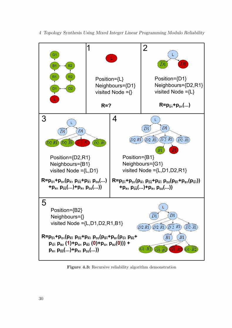
Figure 4.3 shows an illustration of the algorithm for calculating the failure proba-bility at the load for the topology shown at the left corner of the figure. Startingfrom the load (Step 1), we determine the neighboring nodes to be visited in thenext step, then we consider all the possible status for the neighbors (failing / notfailing. If all the neighbors are failing, we add their joint failure probability to thesum making the total failure probability of the system, else we go on exploring thepath starting from the non failing nodes. Once a case where a power source is notfailing is reached, a probability of failure of zero is assigned to that working path. Incase a loop is reached (Step 5), the algorithm does not revisit the previously visitednodes, instead, it propagates a probability equal to one.
28
4.3 Reliability Analysis Framework
Algorithm 2 recReliability
Input: A graph G =(V,E ), the root R of G, P vector of node failure probabilities,C the set of current nodes and W the set of visited nodesOutput: reliability at the root node R (failure probability)
L = []reliability = []for all u in C do % L contains unvisited neighbors of nodes in C
for all v in neighbors(u) doif isnot(v,W ) then
L = [L, v]end if
end forend forW = [W,L]; % Update the previously visited nodes% reliability calculationif isempty(L) then
reliability = 1% check whether there is at least one power source in C, otherwise all the neighborshave been previously visited
for all u in C doif isGenerator(u) then
reliability = 0break
end ifend for
elsefor event = 0 to (2|L| − 1) do
binEvent = bin(event)x=1for all k in L do
if binEvent(position(k))=0 thenx = x ∗ P (k)
elseif isGenerator(k) then
x = 0else
x = x ∗ (1− P (k))end ifC = [C, k]
end ifend forif event! = 0 then
x = x ∗ sum(recReliability(C,P,W ))end ifreliability = [reliability, x]C = []
end forend if
29
4 Topology Synthesis Using Mixed Integer Linear Programming Modulo Reliability
1
3 4
5
2
Position={L}Neighbours={D1}visited Node ={}
R=?
Position={D1}Neighbours={D2,R1}visited Node ={L}
R=pD1+pD1(...)
Position={D2,R1}Neighbours={B1}visited Node ={L,D1}
R=pD1+pD1(pR1 pD2+pR1 pD2(...) +pR1 pD2(...)+pR1 pD2(...))
Position={B1}Neighbours={G1}visited Node ={L,D1,D2,R1}
R=pD1+pD1(pR1 pD2+pR1 pD2(pB1+pB1(pG1)) +pR1 pD2(...)+pR1 pD2(...))
Position={B2}Neighbours={}visited Node ={L,D1,D2,R1,B1}
R=pD1+pD1(pR1 pD2+pR1 pD2(pB1+pB1(pG1 pB2+ pG1 pB2 (1)+pG1 pB2 (0)+pG1 pB2(0))) + pR1 pD2(...)+pR1 pD2(...))
Figure 4.3: Recursive reliability algorithm demonstration
30

4.3 Reliability Analysis Framework
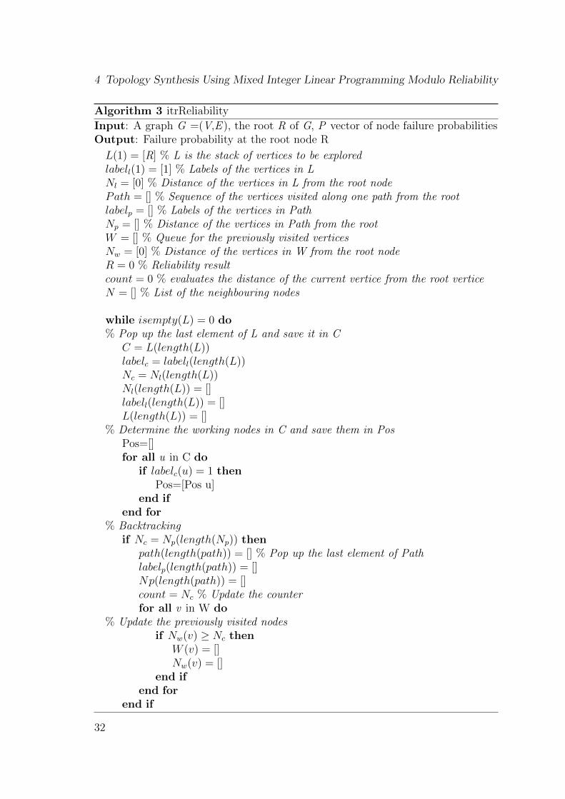
4.3.2 Iterative Algorithm
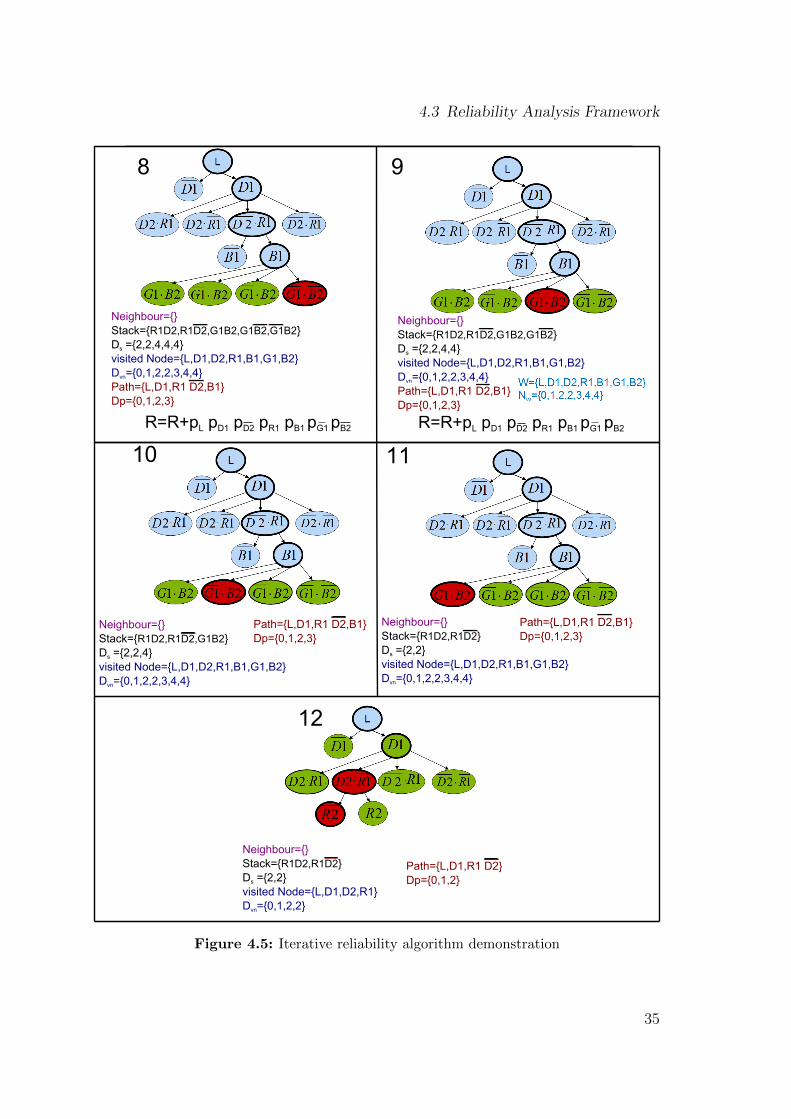
To improve on efficiency, we finally opt for an iterative version (Pseudocode 3) ofthe reliability analysis algorithm. We implement a modification of the Depth FirstSearch algorithm that starts from the first child node of the search tree which consistsof all the failure states of the architecture, and then goes deeper and deeper in eachpath of the tree while adding all the neighbors of the visited nodes, their status (notfailing/failing) and their distance from the root to a stack for exploration, until it hitsa node that has no children. During the search, the algorithm saves the path to theleaves, the status of its nodes (not failing/failing) and their distance from the root. Italso takes account of the previously visited nodes. Nodes with no children can be ofthree types. First, a node with no children can correspond to a working generator,in this case a working path was found and the reliability expression remains thesame. A second alternative is that the node with no children corresponds to a set offailing components. In this case, a failing path was hit, the reliability is expandedwith the probability of failure of that path. The last case correspond to the situationwhere the node with no children has no neighbors that were not previously visited.We add the probability of failure of the path leading to such a node to the totalreliability calculation as well. When the algorithm reaches a node with no childrenand the stack still contains failure events, the search backtracks, returning to themost recent node it has not finished exploring.
31
4 Topology Synthesis Using Mixed Integer Linear Programming Modulo Reliability
Algorithm 3 itrReliability
Input: A graph G =(V,E ), the root R of G, P vector of node failure probabilitiesOutput: Failure probability at the root node R
L(1) = [R] % L is the stack of vertices to be exploredlabell(1) = [1] % Labels of the vertices in LNl = [0] % Distance of the vertices in L from the root nodePath = [] % Sequence of the vertices visited along one path from the rootlabelp = [] % Labels of the vertices in PathNp = [] % Distance of the vertices in Path from the rootW = [] % Queue for the previously visited verticesNw = [0] % Distance of the vertices in W from the root nodeR = 0 % Reliability resultcount = 0 % evaluates the distance of the current vertice from the root verticeN = [] % List of the neighbouring nodes
while isempty(L) = 0 do% Pop up the last element of L and save it in C
C = L(length(L))labelc = labell(length(L))Nc = Nl(length(L))Nl(length(L)) = []labell(length(L)) = []L(length(L)) = []
% Determine the working nodes in C and save them in PosPos=[]for all u in C do
if labelc(u) = 1 thenPos=[Pos u]
end ifend for
% Backtrackingif Nc = Np(length(Np)) then
path(length(path)) = [] % Pop up the last element of Pathlabelp(length(path)) = []Np(length(path)) = []count = Nc % Update the counterfor all v in W do
% Update the previously visited nodesif Nw(v) ≥ Nc then
W (v) = []Nw(v) = []
end ifend for
end if
32
4.3 Reliability Analysis Framework
if isGenerator(Pos) = 0 then% Update W and Nw
if thenW = [W,C]for i=1 to size(C) do
Nw = [Nw, count]end for
% Determine all the neighbours of the nodes in Posfor all u in Pos do
for all v in neighbors(u) doif isnot(v,W ) then
N = [N, v]end if
end forend for
% Evaluate the Reliabilityif labelc = 0 OR N = [] then
x = 1X = [Path, C]for all uinX do
for all vinX(u) doif labelp(u)(v) = 0 then
x = x · P (X(u)(v))else
x = x · (1− P (X(u)(v)))end if
end forReliability = Reliability + x
end forelse
for event = 0 to (2|N | − 1) dobinEvent = bin(event)labell = [labell, binEvent]L = [L, binEvent]Nl = [Nl, count+ 1]
end forPath = [Path, C]labelp = [labelp, labelc]Np = [Np, count]count = count+ 1
end ifend if
33
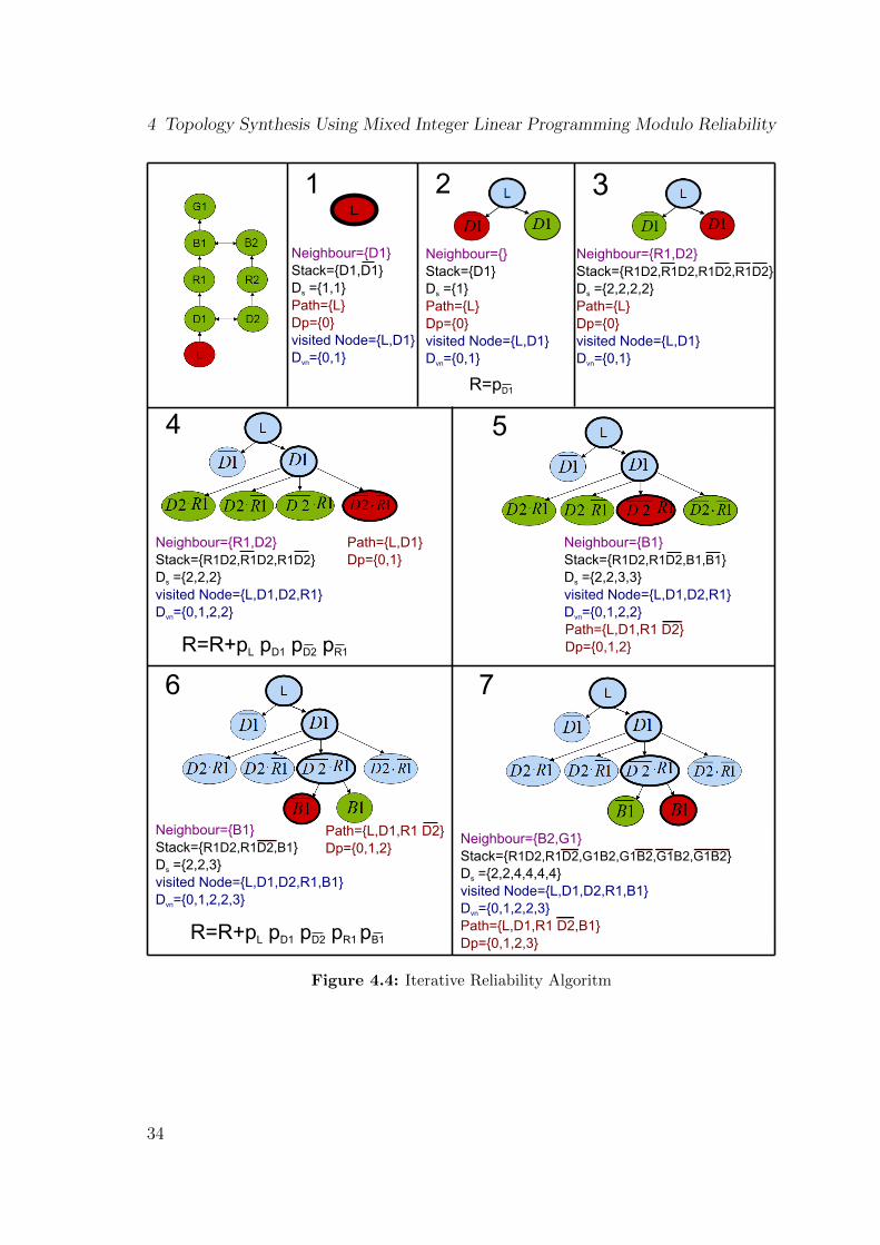
4 Topology Synthesis Using Mixed Integer Linear Programming Modulo Reliability
1 2
4
L
3
4 5
6 7
Neighbour={D1}Stack={D1,D1}Ds0={1,1}Path={L}Dp={0}visited0Node={L,D1}Dvn={0,1}
Neighbour={}Stack={D1}Ds0={1}Path={L}Dp={0}visited0Node={L,D1}Dvn={0,1}
R=pD1
Neighbour={R1,D2}Stack={R1D2,R1D2,R1D2,R1D2}Ds0={2,2,2,2}Path={L}Dp={0}visited0Node={L,D1}Dvn={0,1}
Neighbour={R1,D2}Stack={R1D2,R1D2,R1D2}Ds0={2,2,2}visited0Node={L,D1,D2,R1}Dvn={0,1,2,2}
R=R+pL0pD10pD20pR1
Path={L,D1}Dp={0,1}
Neighbour={B1}Stack={R1D2,R1D2,B1,B1}Ds0={2,2,3,3}visited0Node={L,D1,D2,R1}Dvn={0,1,2,2}Path={L,D1,R10D2}Dp={0,1,2}
Neighbour={B1}Stack={R1D2,R1D2,B1}Ds0={2,2,3}visited0Node={L,D1,D2,R1,B1}Dvn={0,1,2,2,3}
Path={L,D1,R10D2}Dp={0,1,2}
R=R+pL0pD10pD20pR10pB1
Neighbour={B2,G1}Stack={R1D2,R1D2,G1B2,G1B2,G1B2,G1B2}Ds0={2,2,4,4,4,4}visited0Node={L,D1,D2,R1,B1}Dvn={0,1,2,2,3}Path={L,D1,R10D2,B1}Dp={0,1,2,3}
Figure 4.4: Iterative Reliability Algoritm
34
4.3 Reliability Analysis Framework
8 9
10 11
12
Neighbour={}Stack={R1D2,R1D2,G1B2,G1B2,G1B2}Dsd={2,2,4,4,4}visiteddNode={L,D1,D2,R1,B1,G1,B2}Dvn={0,1,2,2,3,4,4}Path={L,D1,R1dD2,B1}Dp={0,1,2,3}
R=R+pLdpD1dpD2dpR1ddpB1dpG1dpB2
Neighbour={}Stack={R1D2,R1D2,G1B2,G1B2}Dsd={2,2,4,4}visiteddNode={L,D1,D2,R1,B1,G1,B2}Dvn={0,1,2,2,3,4,4}Path={L,D1,R1dD2,B1}Dp={0,1,2,3}
R=R+pLdpD1dpD2dpR1ddpB1dpG1dpB2
Neighbour={}Stack={R1D2,R1D2,G1B2}Dsd={2,2,4}visiteddNode={L,D1,D2,R1,B1,G1,B2}Dvn={0,1,2,2,3,4,4}
Path={L,D1,R1dD2,B1}Dp={0,1,2,3}
Neighbour={}Stack={R1D2,R1D2}Dsd={2,2}visiteddNode={L,D1,D2,R1,B1,G1,B2}Dvn={0,1,2,2,3,4,4}
Path={L,D1,R1dD2,B1}Dp={0,1,2,3}
Neighbour={}Stack={R1D2,R1D2}Dsd={2,2}visiteddNode={L,D1,D2,R1}Dvn={0,1,2,2}
Path={L,D1,R1dD2}Dp={0,1,2}
Figure 4.5: Iterative reliability algorithm demonstration
35
4 Topology Synthesis Using Mixed Integer Linear Programming Modulo Reliability
4.4 Strategies to Increase the Reliability
As it was already explained, if the failure probability of the obtained topology ishigher than the required one, more connectivity constraints that increase the degreeof redundancy of the topology are added. For this purpose, we create a library ofdifferent moves, that can be used to increase the reliability. First, we will give anoverview of the moves, then we will explain how we organize them in two differentstrategies.
4.4.1 Moves
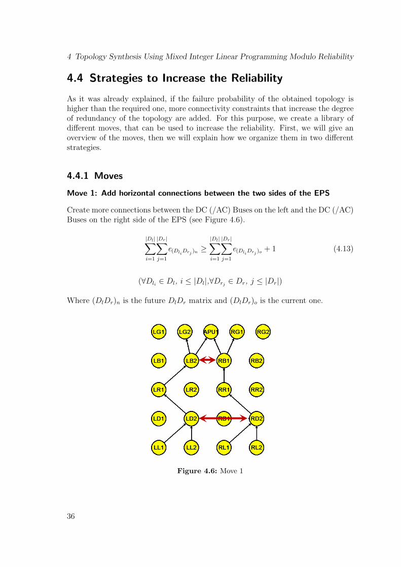
Move 1: Add horizontal connections between the two sides of the EPS
Create more connections between the DC (/AC) Buses on the left and the DC (/AC)Buses on the right side of the EPS (see Figure 4.6).
|Dl|∑i=1
|Dr|∑j=1
e(DliDrj )n
≥|Dl|∑i=1
|Dr|∑j=1
e(DliDrj )o
+ 1 (4.13)
(∀Dli ∈ Dl, i ≤ |Dl|,∀Drj ∈ Dr, j ≤ |Dr|)
Where (DlDr)n is the future DlDr matrix and (DlDr)o is the current one.
Figure 4.6: Move 1
36

4.4 Strategies to Increase the Reliability
Move 2: Add K connections between the left and right side of the EPS
Add a determined number of connections K between the DC (/AC) Buses on theleft and DC (/AC) Buses on the right.
|Dl|∑i=1
|Dr|∑j=1
e(DliDrj)n
=
|Dl|∑i=1
|Dr|∑j=1
e(DliDrj )o
+K (4.14)
(∀Dli ∈ Dl, i ≤ |Dl|,∀Drj ∈ Dr, j ≤ |Dr|)
|Bl|∑i=1
|Br|∑j=1
e(BliBrj )n
=
|Bl|∑i=1
|Br|∑j=1
e(BliBrj )o
+K (4.15)
(∀Bli ∈ Bl, i ≤ |Bl|,∀Brj ∈ Br, j ≤ |Br|)
Where (BlBr)n is the future BlBr matrix, (BlBr)o is the current one, (DlDr)n is thefuture DlDr matrix and (DlDr)o is the current one.
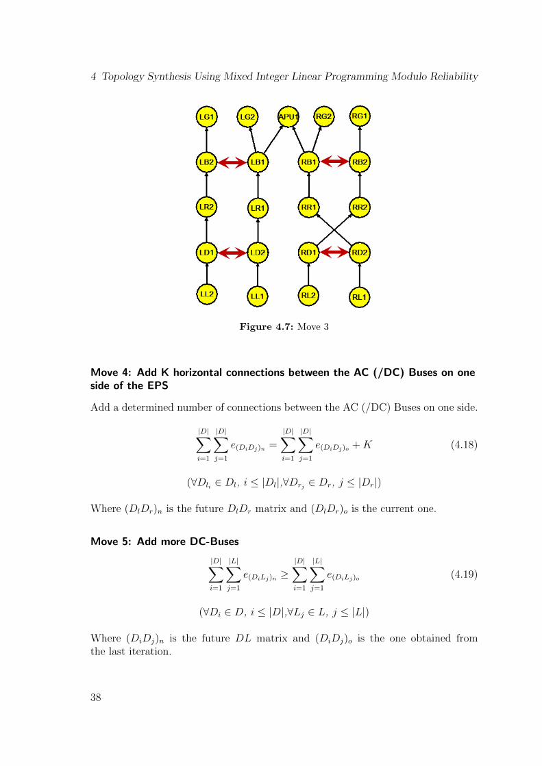
Move 3: Add horizontal connections on one side of the EPS
Add horizontal connections between the AC (/DC) Buses on one side (see Figure4.7).
|D|∑i=1
|D|∑j=1
e(DiDj)n ≥|D|∑i=1
|D|∑j=1
e(DiDj)o + 1 (4.16)
(∀Dli ∈ Dl, i ≤ |Dl|,∀Drj ∈ Dr, j ≤ |Dr|)
|B|∑i=1
|B|∑j=1
e(BiBj)n ≥|B|∑i=1
|B|∑j=1
e(BiBj)o + 1 (4.17)
(∀Bli ∈ Bl, i ≤ |Bl|,∀Brj ∈ Br, j ≤ |Br|)
Where (BlBr)n is the future BlBr matrix, (BlBr)o the BlBr matrix obtained fromthe last iteration, (DlDr)n the future DlDr matrix and (DlDr)o the DlDr matrixobtained from the last iteration.
37
4 Topology Synthesis Using Mixed Integer Linear Programming Modulo Reliability
Figure 4.7: Move 3
Move 4: Add K horizontal connections between the AC (/DC) Buses on oneside of the EPS
Add a determined number of connections between the AC (/DC) Buses on one side.
|D|∑i=1
|D|∑j=1
e(DiDj)n =
|D|∑i=1
|D|∑j=1
e(DiDj)o +K (4.18)
(∀Dli ∈ Dl, i ≤ |Dl|,∀Drj ∈ Dr, j ≤ |Dr|)
Where (DlDr)n is the future DlDr matrix and (DlDr)o is the current one.
Move 5: Add more DC-Buses
|D|∑i=1
|L|∑j=1
e(DiLj)n ≥|D|∑i=1
|L|∑j=1
e(DiLj)o (4.19)
(∀Di ∈ D, i ≤ |D|,∀Lj ∈ L, j ≤ |L|)
Where (DiDj)n is the future DL matrix and (DiDj)o is the one obtained fromthe last iteration.
38
4.4 Strategies to Increase the Reliability
Move 6: Add more rectifiers
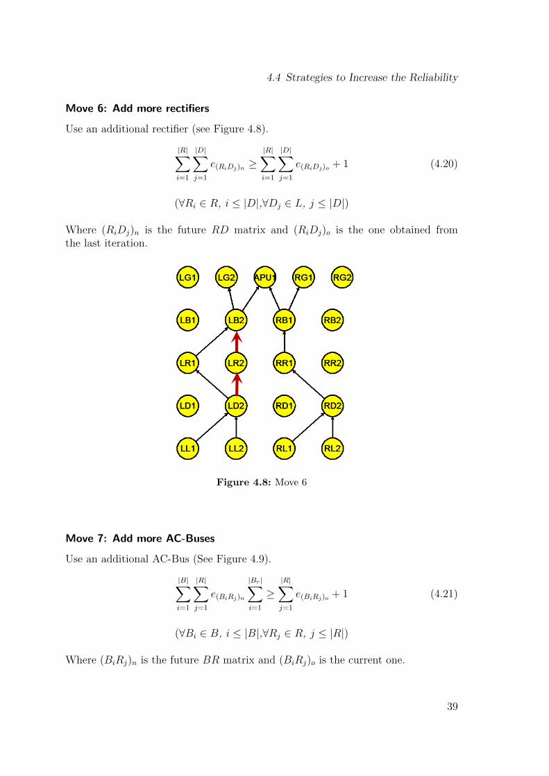
Use an additional rectifier (see Figure 4.8).
|R|∑i=1
|D|∑j=1
e(RiDj)n ≥|R|∑i=1
|D|∑j=1
e(RiDj)o + 1 (4.20)
(∀Ri ∈ R, i ≤ |D|,∀Dj ∈ L, j ≤ |D|)
Where (RiDj)n is the future RD matrix and (RiDj)o is the one obtained fromthe last iteration.
Figure 4.8: Move 6
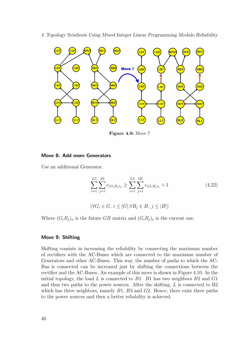
Move 7: Add more AC-Buses
Use an additional AC-Bus (See Figure 4.9).
|B|∑i=1
|R|∑j=1
e(BiRj)n
|Br|∑i=1
≥|R|∑j=1
e(BiRj)o + 1 (4.21)
(∀Bi ∈ B, i ≤ |B|,∀Rj ∈ R, j ≤ |R|)
Where (BiRj)n is the future BR matrix and (BiRj)o is the current one.
39
4 Topology Synthesis Using Mixed Integer Linear Programming Modulo Reliability
Figure 4.9: Move 7
Move 8: Add more Generators
Use an additional Generator.
|G|∑i=1
|B|∑j=1
e(GiBj)n ≥|G|∑i=1
|B|∑j=1
e(GiBj)o + 1 (4.22)
(∀Gi ∈ G, i ≤ |G|,∀Bj ∈ B, j ≤ |B|)
Where (GiBj)n is the future GB matrix and (GiBj)o is the current one.
Move 9: Shifting
Shifting consists in increasing the reliability by connecting the maximum numberof rectifiers with the AC-Buses which are connected to the maximum number ofGenerators and other AC-Buses. This way, the number of paths to which the AC-Bus is connected can be increased just by shifting the connections between therectifier and the AC-Buses. An example of this move is shown in Figure 4.10. In theinitial topology, the load L is connected to B1. B1 has two neighbors B2 and G1and thus two paths to the power sources. After the shifting, L is connected to B2which has three neighbors, namely B1, B3 and G2. Hence, there exist three pathsto the power sources and then a better reliability is achieved.
40
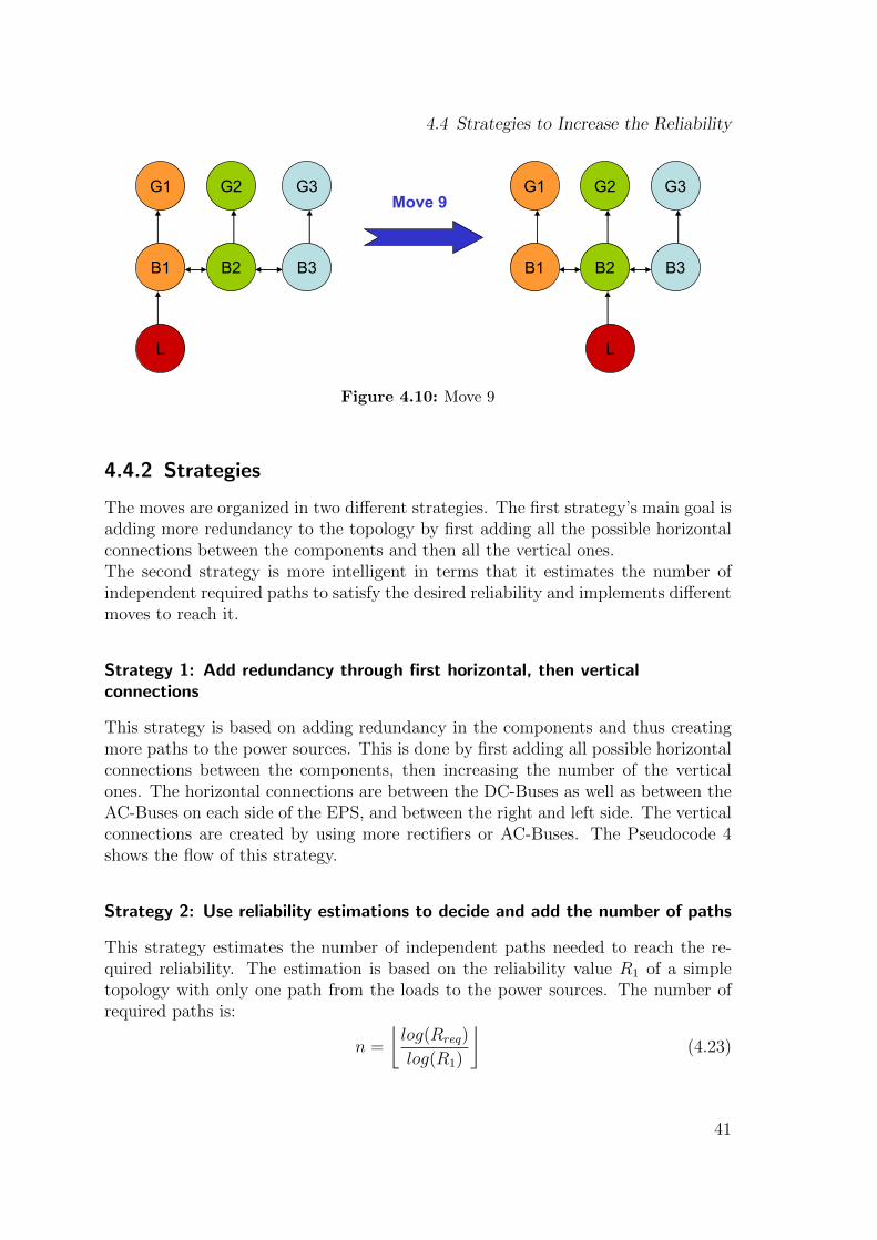
4.4 Strategies to Increase the Reliability
G1 G2 G3
B1 B2 B3
G1 G2 G3
B1 B2 B3
L L
Move 9
Figure 4.10: Move 9
4.4.2 Strategies
The moves are organized in two different strategies. The first strategy’s main goal isadding more redundancy to the topology by first adding all the possible horizontalconnections between the components and then all the vertical ones.The second strategy is more intelligent in terms that it estimates the number ofindependent required paths to satisfy the desired reliability and implements differentmoves to reach it.
Strategy 1: Add redundancy through first horizontal, then verticalconnections
This strategy is based on adding redundancy in the components and thus creatingmore paths to the power sources. This is done by first adding all possible horizontalconnections between the components, then increasing the number of the verticalones. The horizontal connections are between the DC-Buses as well as between theAC-Buses on each side of the EPS, and between the right and left side. The verticalconnections are created by using more rectifiers or AC-Buses. The Pseudocode 4shows the flow of this strategy.
Strategy 2: Use reliability estimations to decide and add the number of paths
This strategy estimates the number of independent paths needed to reach the re-quired reliability. The estimation is based on the reliability value R1 of a simpletopology with only one path from the loads to the power sources. The number ofrequired paths is:
n =
⌊log(Rreq)
log(R1)
⌋(4.23)
41
4 Topology Synthesis Using Mixed Integer Linear Programming Modulo Reliability
Algorithm 4 Strategy1: Strategy 1
Input: A graph G =(V,E )Output: Additional constraints C
if Connected(DL, DR) = 0 thenC = [C,Move1(DL, DR)]
else if Connected(BL, BR) = 0 thenC = [C,Move1(BL, BR)]
else if (Connected(DR) = 0) ∨ (Connected(DL) = 0) thenC = [C,Move3(DR)]C = [C,Move3(DL]
else if (Connected(BR) = 0) ∨ (Connected(Bl) = 0) thenC = [C,Move3(BR)]C = [C,Move3(BL)]
else if Connected(R) = 0 thenC = [C,Move6(R)]
else if Connected(G) = 0 thenC = [C,Move8(G)]
end if=0
The number of paths that can be possibly added is equal to the number of DC-Buses which are connected to rectifiers but not connected to other DC-Buses onboth the right and left sides of the EPS. This is justified by the fact that each DC-Bus potentially starts a new path towards the power sources.In case the number of available paths to be added is not sufficient, we implementdifferent other moves as it is shown in Pseudocode 5.
4.5 Handling Contactors
4.5.1 Generating Switch Connectivity Matrices
Power switches are needed to switch between the different paths of the topology or toshed failing components. We account for the switches in two ways. A first approachassumes switches at each edge and their probabilities was computed under the as-sumption that each switch was in series with a component. As a second approach,switches are handled as independent components, inserted into the adjacency matrixand taken into account in the optimization process. Each two components’ connec-tions are described by a subconnectivity matrix. Each connectivity matrix has itscorresponding switch matrix. If there is no connection between two components(zero in the connectivity matrix), a zero is assigned to the corresponding positionin the switch matrix. If there is a connection between two components (one in theconnectivity matrix) there are two possibilities; either a one in the corresponding
42
4.5 Handling Contactors
Algorithm 5 Strategy 2
Input: A graph G =(V,E ), the required reliability Rreq, the maximum reachedreliability RR on the right side from the first iteration at the DC-Bus DR, themaximum reached reliability RL on the left side from the first iteration at the DC-Bus DL
Output: Additional constraints C
pathR = 0 ( global variable)pathL = 0 ( global variable)
% Determine the required paths on the right and left side of the EPSwhile (RR)pathR > Rreq do
pathR = pathR + 1end whilewhile (RL)pathL > Rreq do
pathL = pathL + 1end while
% Determine the possible paths on the right and left side of the EPS that can beadded to increase the reliabilityPossiblePathr={|DiR||Connected(DiR, RR) = 1 ∧ Connected(DiR, DjR) = 0}PossiblePathl={|DiL|/Connected(DiL, RL) = 1 ∧ Connected(DiL, DjL) = 0}PossiblePathlr = (Connected(DR, DL) = 0)
%Steps to increase the reliability%Step 1: Add all the possible right right, left left and right left connectionsC = [C,Move4(DR, PossiblePathR)]C = [C,Move4(DL, PossiblePathL)]C = [C,Move2(DR, DL, PossiblePathlr)]% Step 2: ShiftingC = [C,Move9(BRR), BRL]% Step 3: If the required reliability is not reached, apply more moves% Add more rectifiersif (Connected(R) = 0) then
C = [C,Move6(R)]% Add horizontal connections between the AC Buseselse if Connected(BR) = 0) ∨ Connected(Bl) = 0) then
C = [C,Move3(BR)]C = [C,Move3(BL)]
% Add more AC Buseselse if Connected(B) = 0 then
C = [C,Move7(B)]% Add more Generatorselse if Connected(G) = 0 then
C = [C,Move8(G)]end if
43

4 Topology Synthesis Using Mixed Integer Linear Programming Modulo Reliability
position in the switch connectivity matrix in case there exists a switch connectionor a zero for the case of a direct connection. The Switch Matrices are generatedaccording to the following rules, that guarantees that failing components can beisolated:
• The Loads always have a physical connection with the DC-Buses
DLs=0 (4.24)
• There must always be a switch between the AC-Buses and the power sources
GBs=GB (4.25)
BAPUs=BAPU (4.26)
• There must always be a switch connection between the left and right side ofthe EPS
BBsLR = BBLR (4.27)
DDsLR = DDLR (4.28)
• There must always be a switch connection between the DC (/AC) Buses onone side
DDsR=DDR (4.29)
DDsL=DDL (4.30)
BBsR=BBR (4.31)
BBsL=BBL (4.32)
• For the rest of the connection, if the component has more than one neighbor,there must be a switch connection between that component and its neighbors,else the component has a physical connection to its unique neighbor.
4.5.2 Extending the Adjacency Matrix
After building the Switch Connectivity Matrices, we generate extended connec-tivity matrices that take the switches into consideration. The transformationfrom the CMs without switches to the new CMs considering the switches isdone by first checking for each connection in the CM, using the SCM whetherit corresponds to a switch or a non switch connection. After determining thenumber and place of the selective and non selective connections, we createthe extended matrices following two strategies depending on whether the CMcorrespond to components with horizontal or vertical connections. Next, weexamine these two different cases.
44

4.5 Handling Contactors
Horizontal Connection (between Components on the Same Level)
In this case we are dealing with AC-AC and DC-DC connections. The BBor DD matrices are extended with rows and columns that correspond to theswitches as it is shown in the example below. We consider an adjacency matrixAm,n and a Switch Matrix Bm,n, where:
Am,n =
( a1 a2
a1 0 1a2 1 0
);Bm,n =
( a1 a2
a1 0 1a2 1 0
)(4.33)
According to the adjacency matrix, there is a connection between a1 anda2. To investigate whether these connections are non selective connectionsor selective ones, we check B(a1, a2) and B(a2, a1) in the switch matrix B.Since B(a1, a2) = B(a2, a1) = 1, the connection between a1 and a2 is a switchconnection. We call S, the switch between a1 and a2. The Adjacency Matrixis extended with one row and one column for the switch S. We call the extendAdjacency Matrix AS with:
ASm,n =
a1 a2 S
a1 0 0 1a2 0 0 1S 1 1 0
(4.34)
Vertical Connection (between Components not on the Same Level)
We consider an Adjacency Matrix Am,n and a Switch Matrix Bm,n, where:
Am,n =
( a1 a2
b1 0 1b2 0 1
);Bm,n =
( a1 a2
b1 0 1b2 0 0
)(4.35)
According to the Adjacency Matrix, there are three connections, the first one isbetween the components b1 and a1, the second one is between the componentsa2 and b1 and the third one is between a2 and b2. To investigate whether theseconnections are selective or non selective, we check B(b1, a2), and B(b2, a2)in the switch matrix B. Since B(b1, a2) = 1, the connection between b1and a2 is a switch connection. We call Sb1a2 , the switch between b1 anda2. B(b1, a2) = 0, then the connection between a2 and b1 is a non selectiveconnection. From the original connectivity matrix A, we obtain two new
45
4 Topology Synthesis Using Mixed Integer Linear Programming Modulo Reliability
connectivity matrices BS and SA as it is shown in the example below:
SAm,n=
(Sb1 1b2 0
)(4.36)
SBm,n=( a1 a2
S 0 1)
(4.37)
4.6 Soundness and Completeness
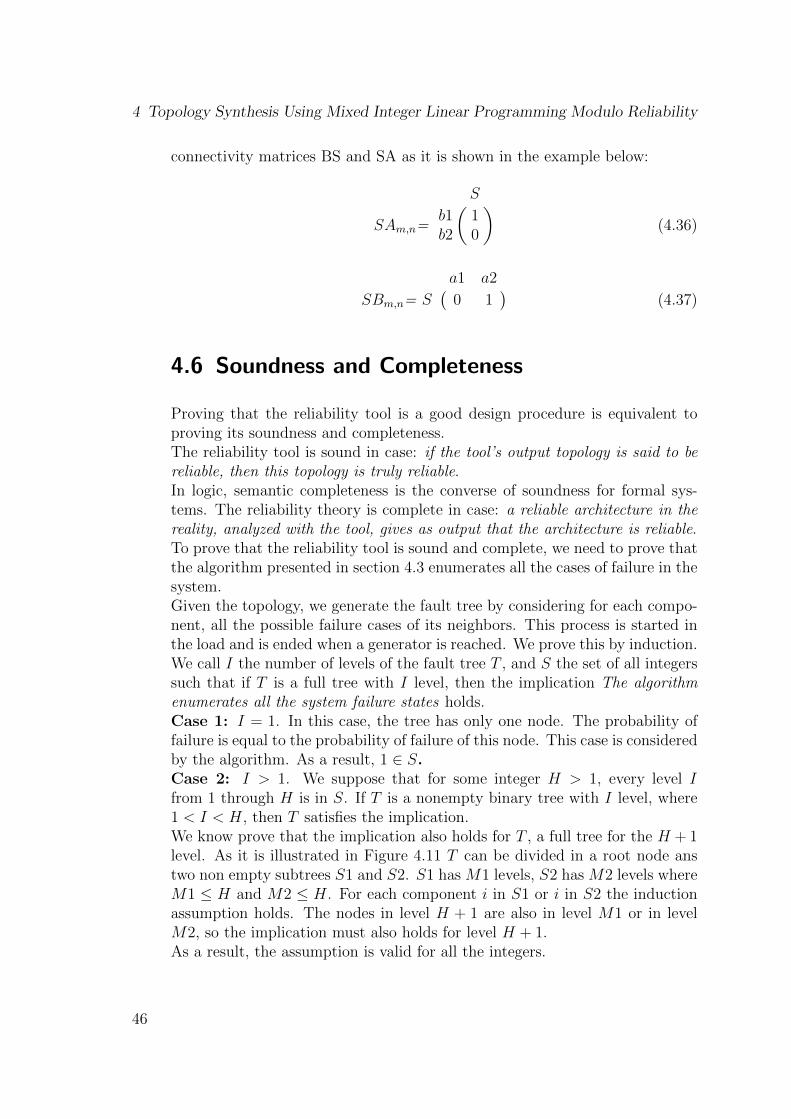
Proving that the reliability tool is a good design procedure is equivalent toproving its soundness and completeness.The reliability tool is sound in case: if the tool’s output topology is said to bereliable, then this topology is truly reliable.In logic, semantic completeness is the converse of soundness for formal sys-tems. The reliability theory is complete in case: a reliable architecture in thereality, analyzed with the tool, gives as output that the architecture is reliable.To prove that the reliability tool is sound and complete, we need to prove thatthe algorithm presented in section 4.3 enumerates all the cases of failure in thesystem.Given the topology, we generate the fault tree by considering for each compo-nent, all the possible failure cases of its neighbors. This process is started inthe load and is ended when a generator is reached. We prove this by induction.We call I the number of levels of the fault tree T , and S the set of all integerssuch that if T is a full tree with I level, then the implication The algorithmenumerates all the system failure states holds.Case 1: I = 1. In this case, the tree has only one node. The probability offailure is equal to the probability of failure of this node. This case is consideredby the algorithm. As a result, 1 ∈ S.Case 2: I > 1. We suppose that for some integer H > 1, every level Ifrom 1 through H is in S. If T is a nonempty binary tree with I level, where1 < I < H, then T satisfies the implication.We know prove that the implication also holds for T , a full tree for the H + 1level. As it is illustrated in Figure 4.11 T can be divided in a root node anstwo non empty subtrees S1 and S2. S1 has M1 levels, S2 has M2 levels whereM1 ≤ H and M2 ≤ H. For each component i in S1 or i in S2 the inductionassumption holds. The nodes in level H + 1 are also in level M1 or in levelM2, so the implication must also holds for level H + 1.As a result, the assumption is valid for all the integers.
46
4.7 Synthesis Results
S1
S2
Level 1
Level H
Level H+1
Figure 4.11: Induction proof for soundness and completness
4.7 Synthesis Results
In this section, we investigate the results obtained after implementing the twostrategies for improving the reliability. Yalmip [17] is a modeling languagefor solving convex and non-convex optimization problems. We use it as aninterface for CPLEX [18], which solves the actual MILP. CPLEX is an IBMsolver used as a linear optimizer that can optimize an objective (here the costfunction) given a vector of constraints. To visualize the obtained topology, agraph visualization software Graphviz is used. Based on the connectivity ma-trix, it represents the components as nodes and the connection between themas edges.The power requirements of the loads as well as the power capability of thegenerators on each side are shown respectively in Table 4.2 and Table 4.1, forthe case of Template 1.For the case of Template 2, the power capability of the generators and thepower requirements of the loads are shown respectively in Table 4.3 and Ta-ble 4.4. Table 4.5 contains the costs of the components. The probabilities offailure considered in this thesis are presented in Table 4.6.
Table 4.1: Power capability of the generators [W] (Template 1)
RG1 RG2 LG1 LG2 APU
7000 8000 7000 8000 1000
We consider the required reliability to be 10−9 at the critical loads. We in-
47
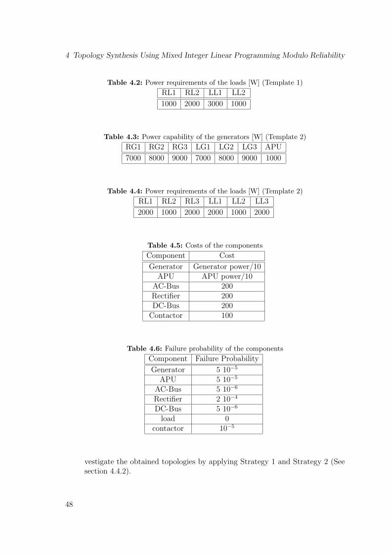
4 Topology Synthesis Using Mixed Integer Linear Programming Modulo Reliability
Table 4.2: Power requirements of the loads [W] (Template 1)
RL1 RL2 LL1 LL2
1000 2000 3000 1000
Table 4.3: Power capability of the generators [W] (Template 2)
RG1 RG2 RG3 LG1 LG2 LG3 APU
7000 8000 9000 7000 8000 9000 1000
Table 4.4: Power requirements of the loads [W] (Template 2)
RL1 RL2 RL3 LL1 LL2 LL3
2000 1000 2000 2000 1000 2000
Table 4.5: Costs of the components
Component Cost
Generator Generator power/10APU APU power/10
AC-Bus 200Rectifier 200DC-Bus 200
Contactor 100
Table 4.6: Failure probability of the components
Component Failure Probability
Generator 5 10−5
APU 5 10−5
AC-Bus 5 10−6
Rectifier 2 10−4
DC-Bus 5 10−6
load 0contactor 10−5
vestigate the obtained topologies by applying Strategy 1 and Strategy 2 (Seesection 4.4.2).
48
4.7 Synthesis Results
4.7.1 Strategy 1
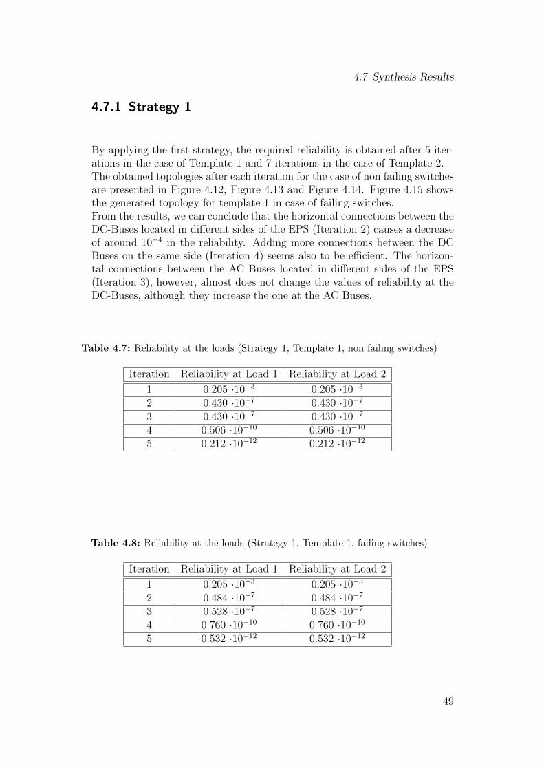
By applying the first strategy, the required reliability is obtained after 5 iter-ations in the case of Template 1 and 7 iterations in the case of Template 2.The obtained topologies after each iteration for the case of non failing switchesare presented in Figure 4.12, Figure 4.13 and Figure 4.14. Figure 4.15 showsthe generated topology for template 1 in case of failing switches.From the results, we can conclude that the horizontal connections between theDC-Buses located in different sides of the EPS (Iteration 2) causes a decreaseof around 10−4 in the reliability. Adding more connections between the DCBuses on the same side (Iteration 4) seems also to be efficient. The horizon-tal connections between the AC Buses located in different sides of the EPS(Iteration 3), however, almost does not change the values of reliability at theDC-Buses, although they increase the one at the AC Buses.
Table 4.7: Reliability at the loads (Strategy 1, Template 1, non failing switches)
Iteration Reliability at Load 1 Reliability at Load 2
1 0.205 ·10−3 0.205 ·10−3
2 0.430 ·10−7 0.430 ·10−7
3 0.430 ·10−7 0.430 ·10−7
4 0.506 ·10−10 0.506 ·10−10
5 0.212 ·10−12 0.212 ·10−12
Table 4.8: Reliability at the loads (Strategy 1, Template 1, failing switches)
Iteration Reliability at Load 1 Reliability at Load 2
1 0.205 ·10−3 0.205 ·10−3
2 0.484 ·10−7 0.484 ·10−7
3 0.528 ·10−7 0.528 ·10−7
4 0.760 ·10−10 0.760 ·10−10
5 0.532 ·10−12 0.532 ·10−12
49
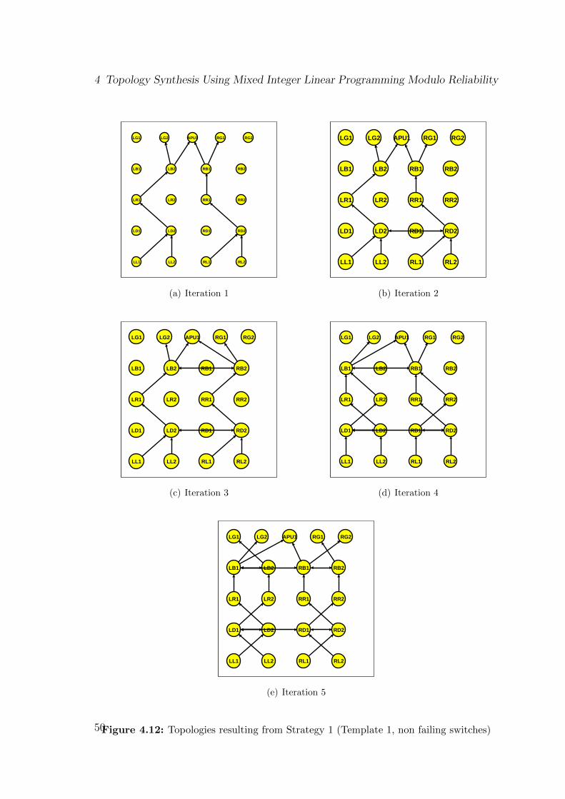
4 Topology Synthesis Using Mixed Integer Linear Programming Modulo Reliability
RG1 RG2
RB1 RB2
RR1 RR2
RD1 RD2
RL1 RL2
APU1LG1 LG2
LB1 LB2
LR1 LR2
LD1 LD2
LL1 LL2
(a) Iteration 1
RG1 RG2
RB1 RB2
RR1 RR2
RD1 RD2
RL1 RL2
APU1LG1 LG2
LB1 LB2
LR1 LR2
LD1 LD2
LL1 LL2
(b) Iteration 2
RG1 RG2
RB1 RB2
RR1 RR2
RD1 RD2
RL1 RL2
APU1LG1 LG2
LB1 LB2
LR1 LR2
LD1 LD2
LL1 LL2
(c) Iteration 3
RG1 RG2
RB1 RB2
RR1 RR2
RD1 RD2
RL1 RL2
APU1LG1 LG2
LB1 LB2
LR1 LR2
LD1 LD2
LL1 LL2
(d) Iteration 4
RG1 RG2
RB1 RB2
RR1 RR2
RD1 RD2
RL1 RL2
APU1LG1 LG2
LB1 LB2
LR1 LR2
LD1 LD2
LL1 LL2
(e) Iteration 5
Figure 4.12: Topologies resulting from Strategy 1 (Template 1, non failing switches)50
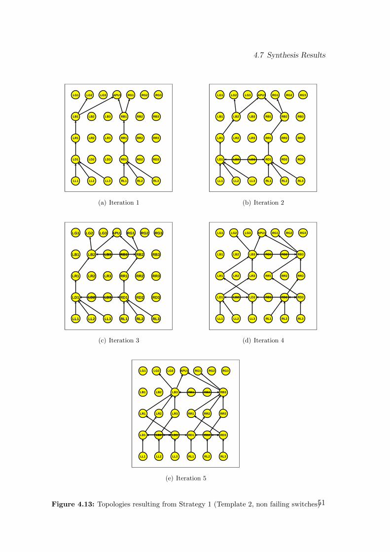
4.7 Synthesis Results
RG1 RG2 RG3
RB1 RB2 RB3
RR1 RR2 RR3
RD1 RD2 RD3
RL1 RL2 RL3
APU1LG1 LG2 LG3
LB1 LB2 LB3
LR1 LR2 LR3
LD1 LD2 LD3
LL1 LL2 LL3
(a) Iteration 1
RG1 RG2 RG3
RB1 RB2 RB3
RR1 RR2 RR3
RD1 RD2 RD3
RL1 RL2 RL3
APU1LG1 LG2 LG3
LB1 LB2 LB3
LR1 LR2 LR3
LD1 LD2 LD3
LL1 LL2 LL3
(b) Iteration 2
RG1 RG2 RG3
RB1 RB2 RB3
RR1 RR2 RR3
RD1 RD2 RD3
RL1 RL2 RL3
APU1LG1 LG2 LG3
LB1 LB2 LB3
LR1 LR2 LR3
LD1 LD2 LD3
LL1 LL2 LL3
(c) Iteration 3
RG1 RG2 RG3
RB1 RB2 RB3
RR1 RR2 RR3
RD1 RD2 RD3
RL1 RL2 RL3
APU1LG1 LG2 LG3
LB1 LB2 LB3
LR1 LR2 LR3
LD1 LD2 LD3
LL1 LL2 LL3
(d) Iteration 4
RG1 RG2 RG3
RB1 RB2 RB3
RR1 RR2 RR3
RD1 RD2 RD3
RL1 RL2 RL3
APU1LG1 LG2 LG3
LB1 LB2 LB3
LR1 LR2 LR3
LD1 LD2 LD3
LL1 LL2 LL3
(e) Iteration 5
Figure 4.13: Topologies resulting from Strategy 1 (Template 2, non failing switches)51
4 Topology Synthesis Using Mixed Integer Linear Programming Modulo Reliability
RG1 RG2 RG3
RB1 RB2 RB3
RR1 RR2 RR3
RD1 RD2 RD3
RL1 RL2 RL3
APU1LG1 LG2 LG3
LB1 LB2 LB3
LR1 LR2 LR3
LD1 LD2 LD3
LL1 LL2 LL3
(a) Iteration 6
RG1 RG2 RG3
RB1 RB2 RB3
RR1 RR2 RR3
RD1 RD2 RD3
RL1 RL2 RL3
APU1LG1 LG2 LG3
LB1 LB2 LB3
LR1 LR2 LR3
LD1 LD2 LD3
LL1 LL2 LL3
(b) Iteration 7
Figure 4.14: Topologies resulting from Strategy 1 (Template 2, non failing switches)
Table 4.9: Reliability at the loads (Strategy 1, Template 2, non failing switches)
Iteration Reliability at Load 1 Reliability at Load 2 Reliability of Load 3
1 0.205 ·10−3 0.205 ·10−3 0.205 ·10−3
2 0.43 ·10−7 0.43 ·10−7 0.43 ·10−7
3 0.43 ·10−7 0.43 ·10−7 0.43 ·10−7
4 0.1 ·10−8 0.1 ·10−8 0.1 ·10−8
5 0.102 ·10−8 0.102 ·10−8 0.102 ·10−8
6 0.102 ·10−8 0.102 ·10−8 0.102 ·10−8
7 0.521 ·10−14 0.521 ·10−14 0.521 ·10−11
52
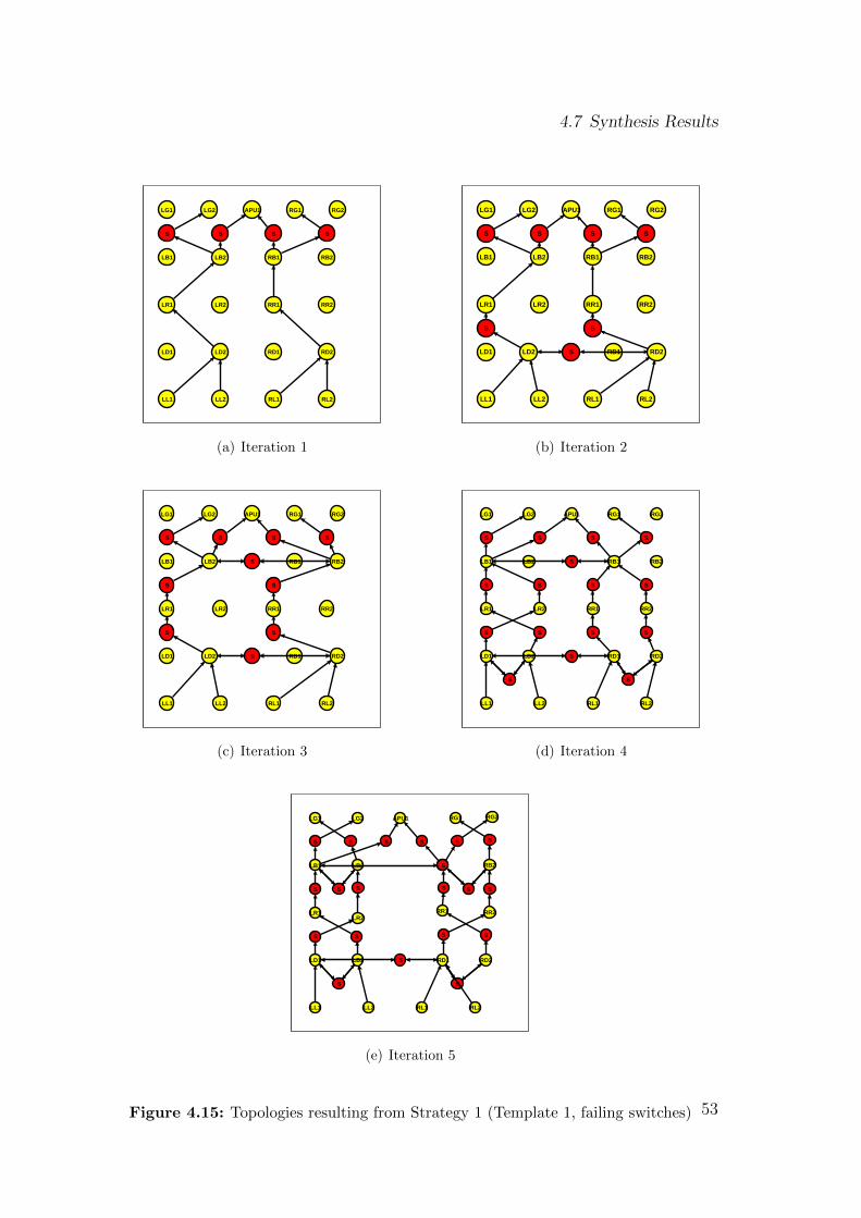
4.7 Synthesis Results
RG1 RG2
S
RB1 RB2
RR1 RR2
RD1 RD2
RL1 RL2
S
APU1
S
LG1 LG2
S
LB1 LB2
LR1 LR2
LD1 LD2
LL1 LL2
(a) Iteration 1
RG1 RG2
S
RB1 RB2
RR1 RR2
S
RD1 RD2
RL1 RL2
S
APU1
S
LG1 LG2
S
LB1 LB2
LR1 LR2
S
LD1 LD2 S
LL1 LL2
(b) Iteration 2
RG1 RG2
S
RB1 RB2
S
RR1 RR2
S
RD1 RD2
RL1 RL2
S
APU1
S
LG1 LG2
S
LB1 LB2 S
S
LR1 LR2
S
LD1 LD2 S
LL1 LL2
(c) Iteration 3
RG1 RG2
S
RB1 RB2
S S
RR1 RR2
S S
RD1 RD2
S
RL1 RL2
S
APU1
S
LG1 LG2
S
LB1 LB2 S
S S
LR1 LR2
S S
LD1 LD2
S
S
LL1 LL2
(d) Iteration 4
S
RB1
RD1 RD2
S
RL1 RL2
S
APU1
S
LG1 LG2
S S
LB1 LB2
S
S
S
LR1
S
LD1 LD2
S
S
LL1 LL2
S S
RR2RR1
S SS
RB2
S
RG1 RG2
S
S
LR2
(e) Iteration 5
Figure 4.15: Topologies resulting from Strategy 1 (Template 1, failing switches) 53
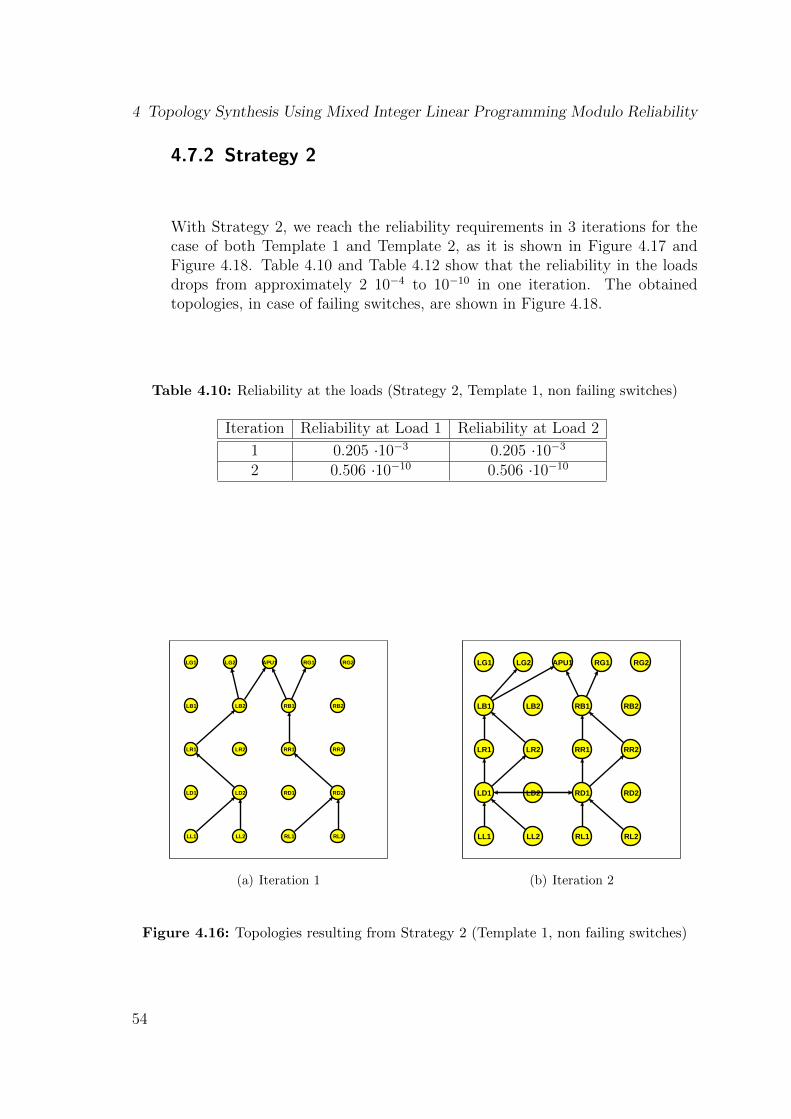
4 Topology Synthesis Using Mixed Integer Linear Programming Modulo Reliability
4.7.2 Strategy 2
With Strategy 2, we reach the reliability requirements in 3 iterations for thecase of both Template 1 and Template 2, as it is shown in Figure 4.17 andFigure 4.18. Table 4.10 and Table 4.12 show that the reliability in the loadsdrops from approximately 2 10−4 to 10−10 in one iteration. The obtainedtopologies, in case of failing switches, are shown in Figure 4.18.
Table 4.10: Reliability at the loads (Strategy 2, Template 1, non failing switches)
Iteration Reliability at Load 1 Reliability at Load 2
1 0.205 ·10−3 0.205 ·10−3
2 0.506 ·10−10 0.506 ·10−10
RG1 RG2
RB1 RB2
RR1 RR2
RD1 RD2
RL1 RL2
APU1LG1 LG2
LB1 LB2
LR1 LR2
LD1 LD2
LL1 LL2
(a) Iteration 1
RG1 RG2
RB1 RB2
RR1 RR2
RD1 RD2
RL1 RL2
APU1LG1 LG2
LB1 LB2
LR1 LR2
LD1 LD2
LL1 LL2
(b) Iteration 2
Figure 4.16: Topologies resulting from Strategy 2 (Template 1, non failing switches)
54
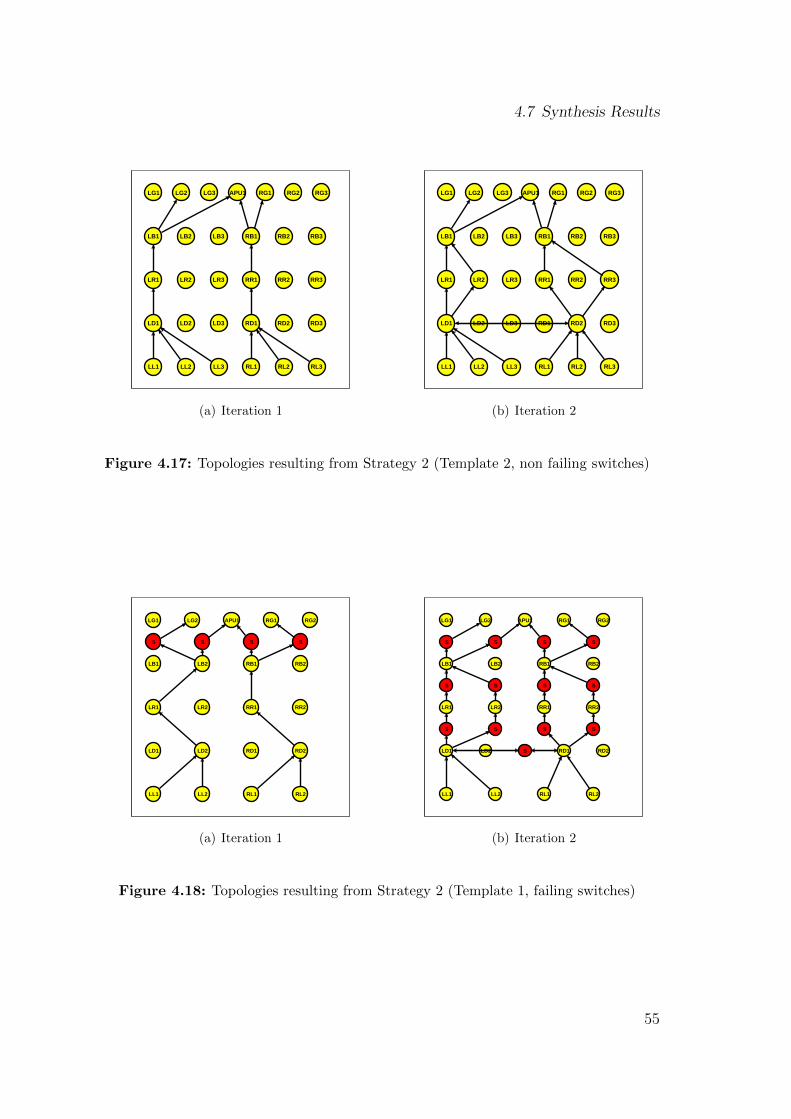
4.7 Synthesis Results
RG1 RG2 RG3
RB1 RB2 RB3
RR1 RR2 RR3
RD1 RD2 RD3
RL1 RL2 RL3
APU1LG1 LG2 LG3
LB1 LB2 LB3
LR1 LR2 LR3
LD1 LD2 LD3
LL1 LL2 LL3
(a) Iteration 1
RG1 RG2 RG3
RB1 RB2 RB3
RR1 RR2 RR3
RD1 RD2 RD3
RL1 RL2 RL3
APU1LG1 LG2 LG3
LB1 LB2 LB3
LR1 LR2 LR3
LD1 LD2 LD3
LL1 LL2 LL3
(b) Iteration 2
Figure 4.17: Topologies resulting from Strategy 2 (Template 2, non failing switches)
RG1 RG2
S
RB1 RB2
RR1 RR2
RD1 RD2
RL1 RL2
S
APU1
S
LG1 LG2
S
LB1 LB2
LR1 LR2
LD1 LD2
LL1 LL2
(a) Iteration 1
RG1 RG2
S
RB1 RB2
S S
RR1 RR2
S S
RD1 RD2
RL1 RL2
S
APU1
S
LG1 LG2
S
LB1 LB2
S S
LR1 LR2
S S
LD1 LD2 S
LL1 LL2
(b) Iteration 2
Figure 4.18: Topologies resulting from Strategy 2 (Template 1, failing switches)
55
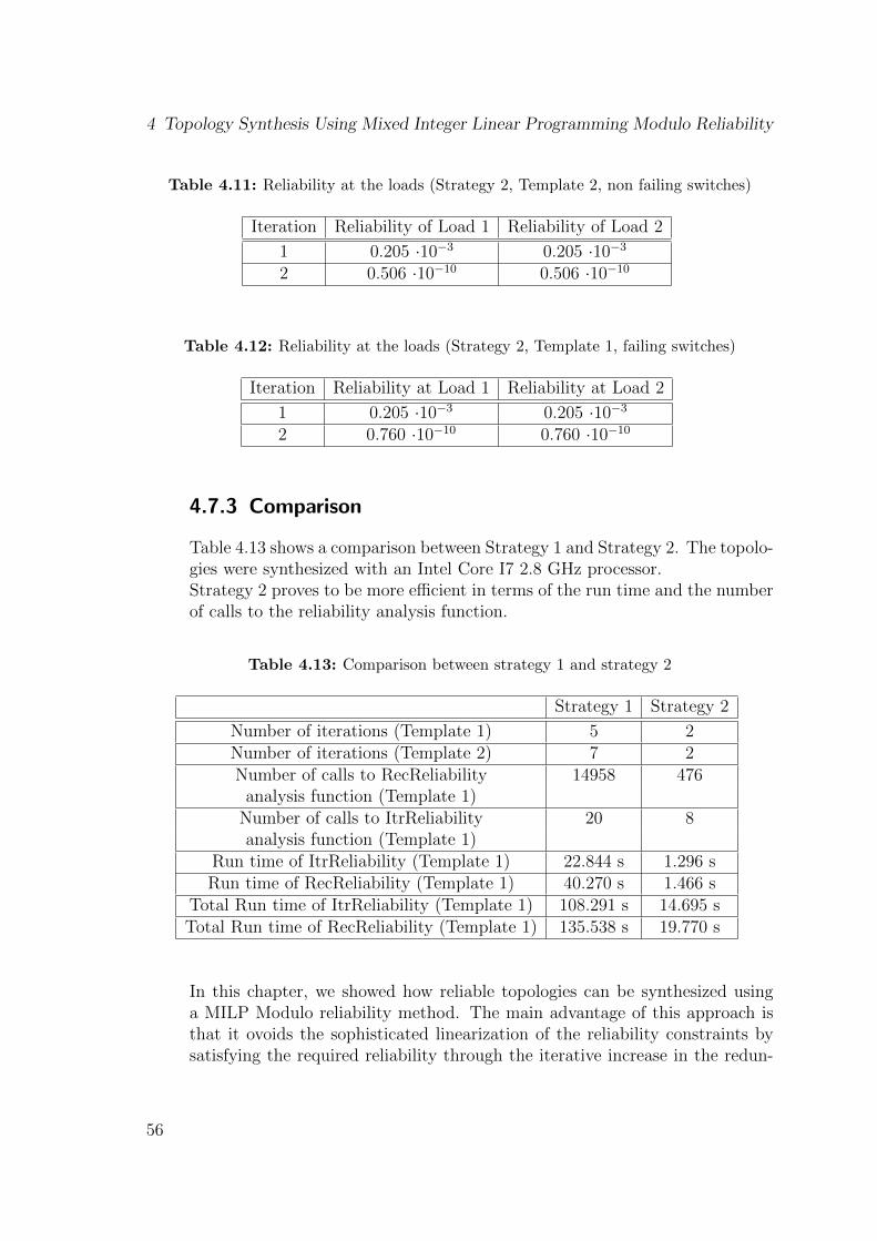
4 Topology Synthesis Using Mixed Integer Linear Programming Modulo Reliability
Table 4.11: Reliability at the loads (Strategy 2, Template 2, non failing switches)
Iteration Reliability of Load 1 Reliability of Load 2
1 0.205 ·10−3 0.205 ·10−3
2 0.506 ·10−10 0.506 ·10−10
Table 4.12: Reliability at the loads (Strategy 2, Template 1, failing switches)
Iteration Reliability at Load 1 Reliability at Load 2
1 0.205 ·10−3 0.205 ·10−3
2 0.760 ·10−10 0.760 ·10−10
4.7.3 Comparison
Table 4.13 shows a comparison between Strategy 1 and Strategy 2. The topolo-gies were synthesized with an Intel Core I7 2.8 GHz processor.Strategy 2 proves to be more efficient in terms of the run time and the numberof calls to the reliability analysis function.
Table 4.13: Comparison between strategy 1 and strategy 2
Strategy 1 Strategy 2
Number of iterations (Template 1) 5 2Number of iterations (Template 2) 7 2Number of calls to RecReliability 14958 476
analysis function (Template 1)Number of calls to ItrReliability 20 8analysis function (Template 1)
Run time of ItrReliability (Template 1) 22.844 s 1.296 sRun time of RecReliability (Template 1) 40.270 s 1.466 s
Total Run time of ItrReliability (Template 1) 108.291 s 14.695 sTotal Run time of RecReliability (Template 1) 135.538 s 19.770 s
In this chapter, we showed how reliable topologies can be synthesized usinga MILP Modulo reliability method. The main advantage of this approach isthat it ovoids the sophisticated linearization of the reliability constraints bysatisfying the required reliability through the iterative increase in the redun-
56

4.7 Synthesis Results
dancy in the topology. However, the obtained solution is suboptimal in termsof the reliability constraints. Another disadvantage is that the run time andthe number of iterations highly depend on the efficiency of the strategy. In thenext chapter, we will explore another approach for generating reliable architec-tures based on symbolic reliability analysis techniques and the manipulationof the reliability constraints.
57

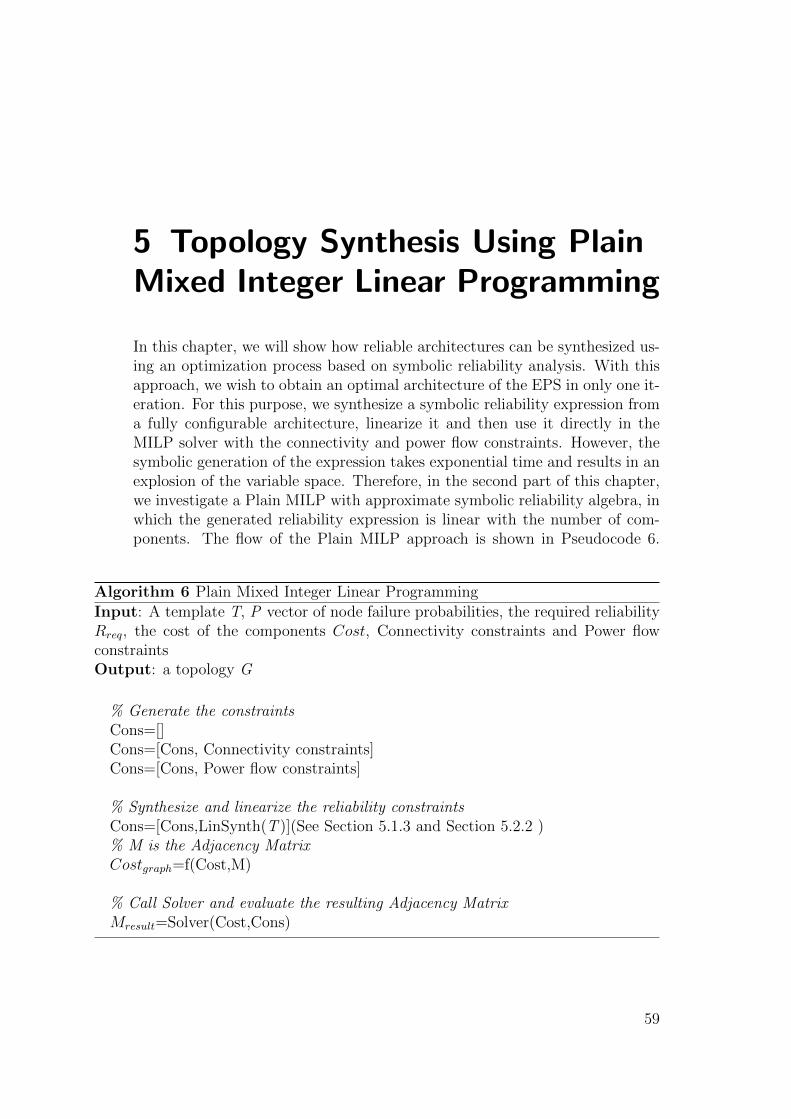
5 Topology Synthesis Using PlainMixed Integer Linear Programming
In this chapter, we will show how reliable architectures can be synthesized us-ing an optimization process based on symbolic reliability analysis. With thisapproach, we wish to obtain an optimal architecture of the EPS in only one it-eration. For this purpose, we synthesize a symbolic reliability expression froma fully configurable architecture, linearize it and then use it directly in theMILP solver with the connectivity and power flow constraints. However, thesymbolic generation of the expression takes exponential time and results in anexplosion of the variable space. Therefore, in the second part of this chapter,we investigate a Plain MILP with approximate symbolic reliability algebra, inwhich the generated reliability expression is linear with the number of com-ponents. The flow of the Plain MILP approach is shown in Pseudocode 6.
Algorithm 6 Plain Mixed Integer Linear Programming
Input: A template T, P vector of node failure probabilities, the required reliabilityRreq, the cost of the components Cost, Connectivity constraints and Power flowconstraintsOutput: a topology G
% Generate the constraintsCons=[]Cons=[Cons, Connectivity constraints]Cons=[Cons, Power flow constraints]
% Synthesize and linearize the reliability constraintsCons=[Cons,LinSynth(T )](See Section 5.1.3 and Section 5.2.2 )% M is the Adjacency MatrixCostgraph=f(Cost,M)
% Call Solver and evaluate the resulting Adjacency MatrixMresult=Solver(Cost,Cons)
59

5 Topology Synthesis Using Plain Mixed Integer Linear Programming
Configurable Topology
Probability Expression
MILP
ProbabilityExpression
Synthesis
Linearization
Figure 5.1: Topology Synthesis Flow (Plain MILP)
5.1 Plain MILP with Exact Reliability Algebra
In this section, we present techniques for the synthesis and of a symbolicreliability expression.
5.1.1 Synthesis of the Reliability Expression
The probability of failure of each components is expressed in terms of theedges connecting it to all its potential neighbors. To generate the symbolicexpression, we use the iterative algorithm with some modifications consistingmainly in considering extra cases, where the edges between a component andits neighbors can be present or non present. We illustrate this process throughthe example discussed in Section 5.1.3.We consider a template with only one column of components and start byassuming a fully connected topology. Since we know that there are no possibleconnections between the components that are not on consecutive levels (e.g.generators and DC-Buses), we obtain the topology shown in Figure 5.2.For each components A, B and C on consecutive levels, we define the proba-bility of failure of A to be RA = pA + RAB, i.e A fails or the connection eABbetween A and B does not exist, or in case of an existing connection, B fails orB does not fail and the failure is caused by the connections or the neighboringcomponents.
RAB = (1− eAB) + eAB(P (B) + (1− P (B))(RBC)) (5.1)
By applying this formula for all the levels, we determine the reliability ex-pression at the critical loads, assuming that they have a probability of failureequal to zero:
RLD = (1− eLD) + eLD(P (D) + (1− P (D))(RDR))RDR = (1− eDR) + eDR(P (R) + (1− P (R))(RRB))RRB = (1− eRB) + eRB(P (B) + (1− P (B))(RBG))RBG = (1− eBG) + eBG(P (G)))
60
5.1 Plain MILP with Exact Reliability Algebra
The expanded synthesized reliability expression at the loads level is:
R = (1− eLD) + eLD(P (D) + (1− P (D))(1− eDR)
+eDR(P (R) + (1− P (R))(1− eRB) + eRB(P (B) (5.3)
+(1− P (B))(1− eBG) + eBG(P (G))))))
Figure 5.2: Topology used to illustrate the symbolic synthesis of reliability expressions
5.1.2 Linearization of the Reliability Expression
A it is shown in equation 5.4, the synthesized reliability expression is non-linear because of the product of the decision variables. In this paragraph,we present techniques to linearize the product as well as the disjunction ofdecision variables.
Linearization of the Product of Binary Variables
The product z = x · y, where both x and y are binary can be easily linearizedby replacing it with the three inequalities below:
z ≤ x (5.4)
z ≤ y (5.5)
z ≥ x+ y − 1 (5.6)
61
5 Topology Synthesis Using Plain Mixed Integer Linear Programming
The first two inequalities ensure that z will be zero if either x or y are zero.The last inequality guarantees that z will take the value 1 if both binaryvariables are set to 1. We can generalize this for a product of n variablesz = x1 · x2 · · · · xn. In this case, z is linearized by adding n+ 1 equations:
z ≤ xi ∀i ∈ {1 · · ·n}
z ≥n∑i=1
xi − n+ 1 (5.7)
ProofWe can prove (5.6) by checking it for all the combinations of xi.case 1: xi = 0 ∀i ∈ {1 · · ·n}. z is equal to 0. The n first inequalities areequivalent to (z ≤ 0), which implies that z is equal to 0. The last inequalityis equal to (z ≥ 1 − n). This implies that z is either negative or equal to 0.Since z is binary, the only possibility is z equal to 0.case 2: xi = 1 ∀i ∈ {1 · · ·n})In this case, z is equal to 1. The n first inequalities are equivalent to z ≤ 1.The last inequality is equal to z ≥ 1, which implies that z is equal to 1.case 3: z is a mixed product of 0 and 1. In this case, z is equal to 0. Then first inequalities are equivalent to either z ≤ 1 or z ≤ 0. This implies thatz should be equal to 0. The last inequality is equal to z ≥ k − n + 1 withk ≤ n− 1. This implies z ≤ 0. Hence, z is equal to 0.
Linearization of the Disjunction of Binary Variables
The product z =n∨i=1
xi, where xi are binary independent variables, can be
transformed by using De Morgan law.
z =n∨i=1
xi
= 1−n∧i=1
(1− xi)
= 1−n∏i=1
(1− xi)
(5.8)
we call a new variable w = (1−x) · (1−y). We use the same method discussedpreviously for the linearization of w.
62
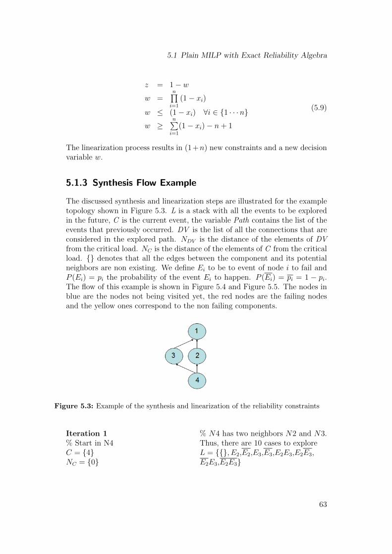
5.1 Plain MILP with Exact Reliability Algebra
z = 1− ww =
n∏i=1
(1− xi)
w ≤ (1− xi) ∀i ∈ {1 · · ·n}w ≥
n∑i=1
(1− xi)− n+ 1
(5.9)
The linearization process results in (1+n) new constraints and a new decisionvariable w.
5.1.3 Synthesis Flow Example
The discussed synthesis and linearization steps are illustrated for the exampletopology shown in Figure 5.3. L is a stack with all the events to be exploredin the future, C is the current event, the variable Path contains the list of theevents that previously occurred. DV is the list of all the connections that areconsidered in the explored path. NDV is the distance of the elements of DVfrom the critical load. NC is the distance of the elements of C from the criticalload. {} denotes that all the edges between the component and its potentialneighbors are non existing. We define Ei to be to event of node i to fail andP (Ei) = pi the probability of the event Ei to happen. P (Ei) = pi = 1 − pi.The flow of this example is shown in Figure 5.4 and Figure 5.5. The nodes inblue are the nodes not being visited yet, the red nodes are the failing nodesand the yellow ones correspond to the non failing components.
Figure 5.3: Example of the synthesis and linearization of the reliability constraints
Iteration 1% Start in N4C = {4}NC = {0}
% N4 has two neighbors N2 and N3.Thus, there are 10 cases to exploreL = {{}, E2,E2,E3,E3,E2E3,E2E3,E2E3,E2E3}
63
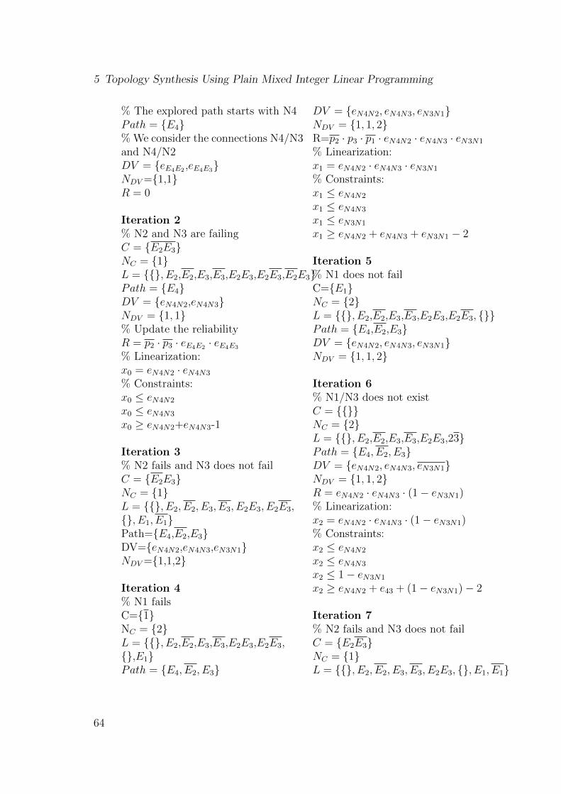
5 Topology Synthesis Using Plain Mixed Integer Linear Programming
% The explored path starts with N4Path = {E4}% We consider the connections N4/N3and N4/N2DV = {eE4E2 ,eE4E3}NDV ={1,1}R = 0
Iteration 2% N2 and N3 are failingC = {E2E3}NC = {1}L = {{}, E2,E2,E3,E3,E2E3,E2E3,E2E3}Path = {E4}DV = {eN4N2,eN4N3}NDV = {1, 1}% Update the reliabilityR = p2 · p3 · eE4E2 · eE4E3
% Linearization:x0 = eN4N2 · eN4N3
% Constraints:x0 ≤ eN4N2
x0 ≤ eN4N3
x0 ≥ eN4N2+eN4N3-1
Iteration 3% N2 fails and N3 does not failC = {E2E3}NC = {1}L = {{}, E2, E2, E3, E3, E2E3, E2E3,{}, E1, E1}Path={E4,E2,E3}DV={eN4N2,eN4N3,eN3N1}NDV ={1,1,2}
Iteration 4% N1 failsC={1}NC = {2}L = {{}, E2,E2,E3,E3,E2E3,E2E3,{},E1}Path = {E4, E2, E3}
DV = {eN4N2, eN4N3, eN3N1}NDV = {1, 1, 2}R=p2 · p3 · p1 · eN4N2 · eN4N3 · eN3N1
% Linearization:x1 = eN4N2 · eN4N3 · eN3N1
% Constraints:x1 ≤ eN4N2
x1 ≤ eN4N3
x1 ≤ eN3N1
x1 ≥ eN4N2 + eN4N3 + eN3N1 − 2
Iteration 5% N1 does not failC={E1}NC = {2}L = {{}, E2,E2,E3,E3,E2E3,E2E3, {}}Path = {E4,E2,E3}DV = {eN4N2, eN4N3, eN3N1}NDV = {1, 1, 2}
Iteration 6% N1/N3 does not existC = {{}}NC = {2}L = {{}, E2,E2,E3,E3,E2E3,23}Path = {E4, E2, E3}DV = {eN4N2, eN4N3, eN3N1}NDV = {1, 1, 2}R = eN4N2 · eN4N3 · (1− eN3N1)% Linearization:x2 = eN4N2 · eN4N3 · (1− eN3N1)% Constraints:x2 ≤ eN4N2
x2 ≤ eN4N3
x2 ≤ 1− eN3N1
x2 ≥ eN4N2 + e43 + (1− eN3N1)− 2
Iteration 7% N2 fails and N3 does not failC = {E2E3}NC = {1}L = {{}, E2, E2, E3, E3, E2E3, {}, E1, E1}
64

5.1 Plain MILP with Exact Reliability Algebra
Path = {E4}DV = {eN4N2, eN4N3, eN2N1}NDV = {1, 1, 2}
Iteration 8% N1 failsC = {E1}L = {{}, E2, E2, E3, E3, E2E3, {}, E1}Path = {E4, E2, E3}DV = {eN4N2, eN4N3, eN2N1}NDV = {1, 1, 2}R = p3 · p2 · p1 · eN4N2 · eN4N3 · eN2N1
% Linearization:x3 = eN4N2 · eN4N3 · eN2N1
% Constraints:x3 ≤ eN4N2
x3 ≤ eN4N3
x3 ≤ eN2N1
x3≥eN4N2 + eN4N3 + eN2N1 − 2
Iteration 9% N1 does not failC = {E1}NC = {2}L = {{}, E2, E2, E3, E3, E2E3, {}}Path = {E4, E2E3}DV = {eN4N2, eN4N3, eN2N1}NDV = {1, 1, 2}
Iteration 10% N1/N2 does not existC = {{}}NC = {2}L = {{}, E2, E2, E3, E3, E2E3}Path = {E4, E2E3}DV = {eN4N2, eN4N3, eN2N1}NDV = {1, 1, 2}R = eN4N2 · eN4N3 · (1− eN2N1)% Linearization:x4 = eN4N2 · eN4N3 · (1− eN2N1)% Constraints:x4 ≤ eN4N2
x4 ≤ eN4N3
x4 ≤ 1− eN2N1
x4 ≥ eN4N2 + eN4N3 + (1− eN2N1)− 2
Iteration 11% N2 and N3 do not failC = {E2E3}NC = {1}L = {{}, E2, E2, E3, E3, {}, E1, E1}Path = {E4}DV = {eN4N2, eN4N3, eN2N1 ∨ eN3N1}NDV = {1, 1, 2}
Iteration 12% N1 failsC = {E1}L = {{}, E2, E2, E3, E3, {}, E1}Path = {E4, E2E3}DV = {eN4N2, eN4N3, eN2N1 ∨ eN3N1}NDV = {1, 1, 2}R = p3 ·p2 ·p1 · eN4N2 · eN4N3 · (eN2N1∨eN3N1)% Linearization:x5 = (eN2N1 ∨ eN3N1)x6 = eN4N2 · eN4N3 · (eN2N1 ∨ eN3N1)% Constraints:x5 ≤ eN2N1
x5 ≤ eN3N1
x5 ≥ eN2N1 + eN3N1 − 1x6 ≤ eN4N2
x6 ≤ eN4N3
x6 ≤ x3x6 ≥ eN4N2 + eN4N3 + (1− x5)− 2
Iteration 13% N1 does not failC = {E1}NC = {2}L = {{}, E2, E2, E3, E3, {}}Path = {E4, E2E3}DV = {eN4N2, eN4N3, eN2N1 ∨ eN3N1}NDV = {1, 1, 2}
65
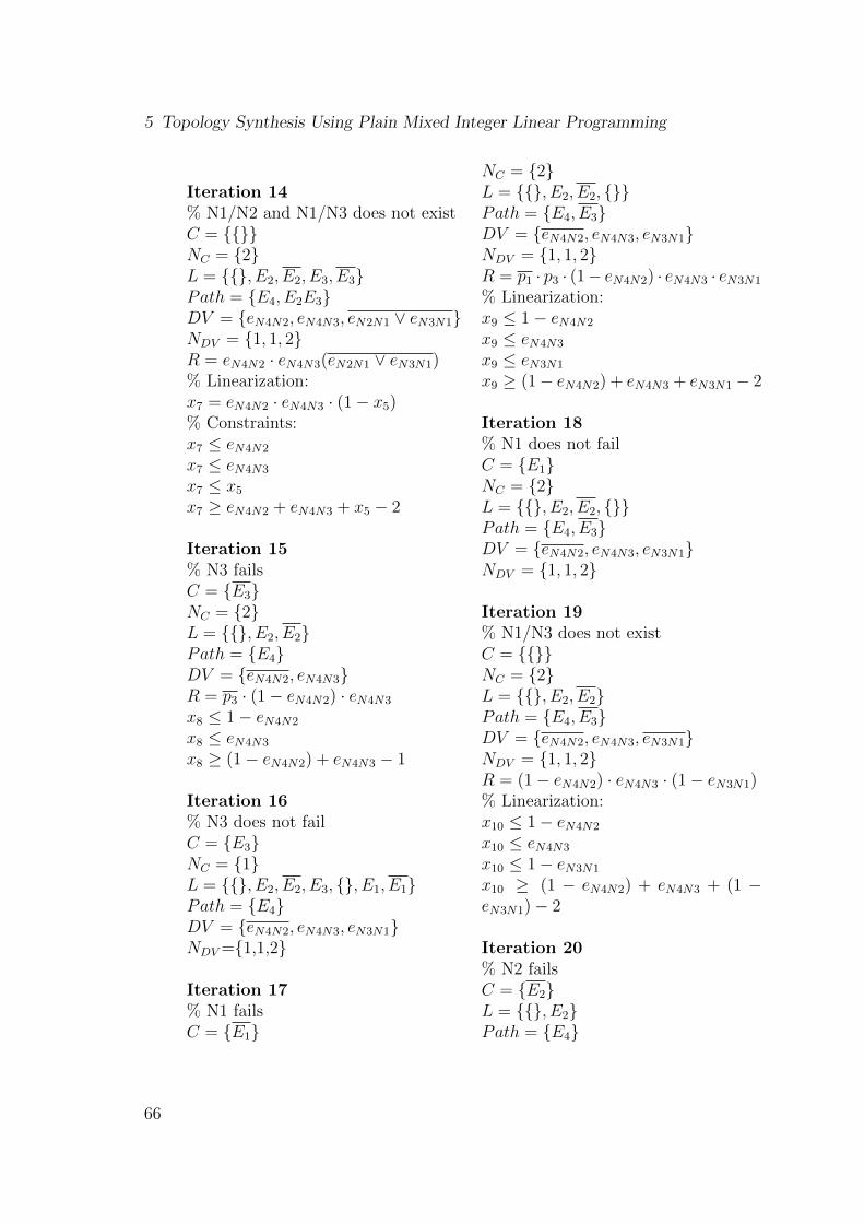
5 Topology Synthesis Using Plain Mixed Integer Linear Programming
Iteration 14% N1/N2 and N1/N3 does not existC = {{}}NC = {2}L = {{}, E2, E2, E3, E3}Path = {E4, E2E3}DV = {eN4N2, eN4N3, eN2N1 ∨ eN3N1}NDV = {1, 1, 2}R = eN4N2 · eN4N3(eN2N1 ∨ eN3N1)% Linearization:x7 = eN4N2 · eN4N3 · (1− x5)% Constraints:x7 ≤ eN4N2
x7 ≤ eN4N3
x7 ≤ x5x7 ≥ eN4N2 + eN4N3 + x5 − 2
Iteration 15% N3 failsC = {E3}NC = {2}L = {{}, E2, E2}Path = {E4}DV = {eN4N2, eN4N3}R = p3 · (1− eN4N2) · eN4N3
x8 ≤ 1− eN4N2
x8 ≤ eN4N3
x8 ≥ (1− eN4N2) + eN4N3 − 1
Iteration 16% N3 does not failC = {E3}NC = {1}L = {{}, E2, E2, E3, {}, E1, E1}Path = {E4}DV = {eN4N2, eN4N3, eN3N1}NDV ={1,1,2}
Iteration 17% N1 failsC = {E1}
NC = {2}L = {{}, E2, E2, {}}Path = {E4, E3}DV = {eN4N2, eN4N3, eN3N1}NDV = {1, 1, 2}R = p1 · p3 · (1− eN4N2) · eN4N3 · eN3N1
% Linearization:x9 ≤ 1− eN4N2
x9 ≤ eN4N3
x9 ≤ eN3N1
x9 ≥ (1− eN4N2) + eN4N3 + eN3N1 − 2
Iteration 18% N1 does not failC = {E1}NC = {2}L = {{}, E2, E2, {}}Path = {E4, E3}DV = {eN4N2, eN4N3, eN3N1}NDV = {1, 1, 2}
Iteration 19% N1/N3 does not existC = {{}}NC = {2}L = {{}, E2, E2}Path = {E4, E3}DV = {eN4N2, eN4N3, eN3N1}NDV = {1, 1, 2}R = (1− eN4N2) · eN4N3 · (1− eN3N1)% Linearization:x10 ≤ 1− eN4N2
x10 ≤ eN4N3
x10 ≤ 1− eN3N1
x10 ≥ (1 − eN4N2) + eN4N3 + (1 −eN3N1)− 2
Iteration 20% N2 failsC = {E2}L = {{}, E2}Path = {E4}
66
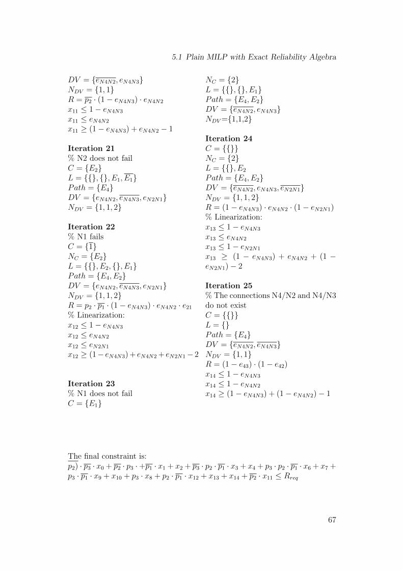
5.1 Plain MILP with Exact Reliability Algebra
DV = {eN4N2, eN4N3}NDV = {1, 1}R = p2 · (1− eN4N3) · eN4N2
x11 ≤ 1− eN4N3
x11 ≤ eN4N2
x11 ≥ (1− eN4N3) + eN4N2 − 1
Iteration 21% N2 does not failC = {E2}L = {{}, {}, E1, E1}Path = {E4}DV = {eN4N2, eN4N3, eN2N1}NDV = {1, 1, 2}
Iteration 22% N1 failsC = {1}NC = {E2}L = {{}, E2, {}, E1}Path = {E4, E2}DV = {eN4N2, eN4N3, eN2N1}NDV = {1, 1, 2}R = p2 · p1 · (1− eN4N3) · eN4N2 · e21% Linearization:x12 ≤ 1− eN4N3
x12 ≤ eN4N2
x12 ≤ eN2N1
x12 ≥ (1− eN4N3) + eN4N2 + eN2N1− 2
Iteration 23% N1 does not failC = {E1}
NC = {2}L = {{}, {}, E1}Path = {E4, E2}DV = {eN4N2, eN4N3}NDV ={1,1,2}
Iteration 24C = {{}}NC = {2}L = {{}, E2
Path = {E4, E2}DV = {eN4N2, eN4N3, eN2N1}NDV = {1, 1, 2}R = (1− eN4N3) · eN4N2 · (1− eN2N1)% Linearization:x13 ≤ 1− eN4N3
x13 ≤ eN4N2
x13 ≤ 1− eN2N1
x13 ≥ (1 − eN4N3) + eN4N2 + (1 −eN2N1)− 2
Iteration 25% The connections N4/N2 and N4/N3do not existC = {{}}L = {}Path = {E4}DV = {eN4N2, eN4N3}NDV = {1, 1}R = (1− e43) · (1− e42)x14 ≤ 1− eN4N3
x14 ≤ 1− eN4N2
x14 ≥ (1− eN4N3) + (1− eN4N2)− 1
The final constraint is:p2) · p3 · x0 + p2 · p3 ·+p1 · x1 + x2 + p3 · p2 · p1 · x3 + x4 + p3 · p2 · p1 · x6 + x7 +p3 · p1 · x9 + x10 + p3 · x8 + p2 · p1 · x12 + x13 + x14 + p2 · x11 ≤ Rreq
67
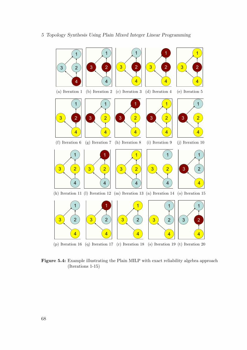
5 Topology Synthesis Using Plain Mixed Integer Linear Programming
1
4
23
(a) Iteration 1
1
4
23
(b) Iteration 2
1
4
23
(c) Iteration 3
1
4
23
(d) Iteration 4
1
4
23
(e) Iteration 5
1
4
23
(f) Iteration 6
1
4
23
(g) Iteration 7
1
4
23
(h) Iteration 8
1
4
23
(i) Iteration 9
1
4
23
(j) Iteration 10
1
4
23
(k) Iteration 11
1
4
23
(l) Iteration 12
1
4
23
(m) Iteration 13
1
4
23
(n) Iteration 14
1
4
23
(o) Iteration 15
1
4
23
(p) Iteration 16
1
4
23
(q) Iteration 17
1
4
23
(r) Iteration 18
1
4
23
(s) Iteration 19
1
4
23
(t) Iteration 20
Figure 5.4: Example illustrating the Plain MILP with exact reliability algebra approach(Iterations 1-15)
68
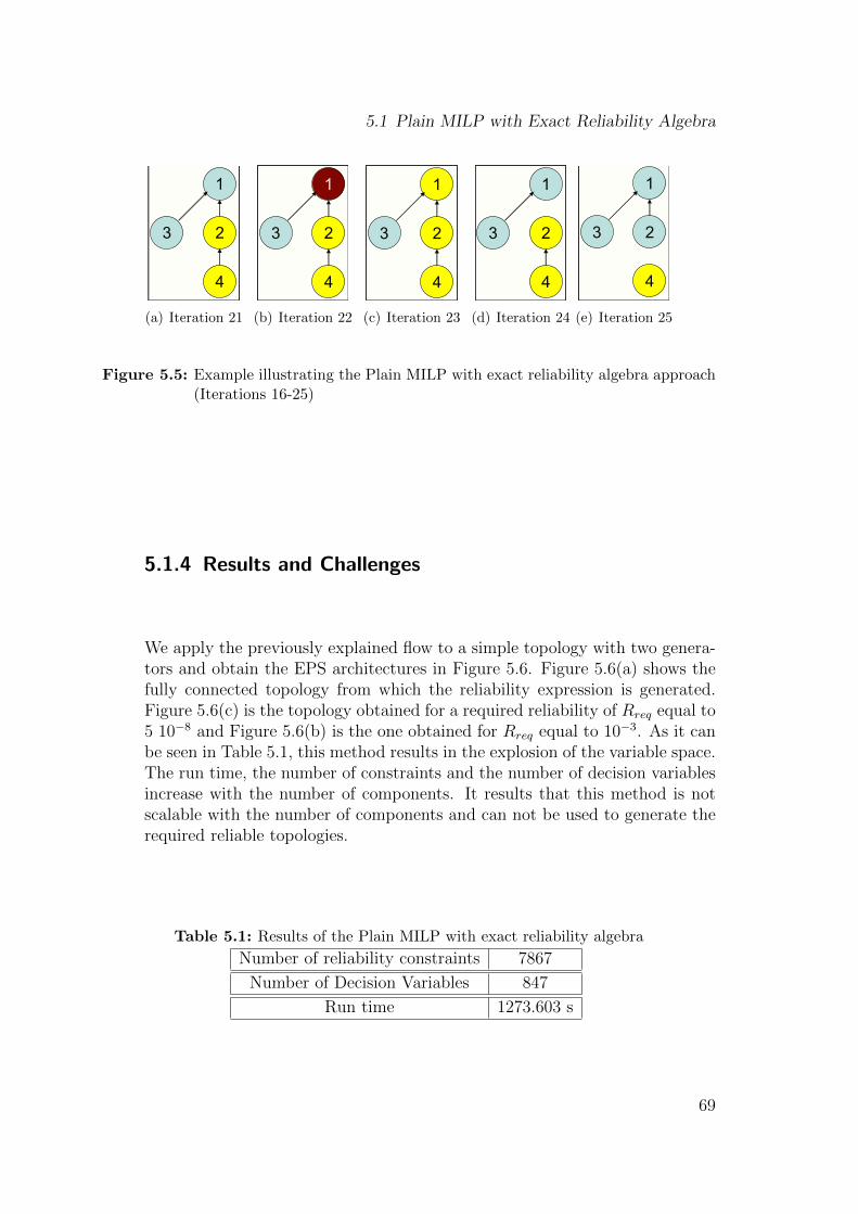
5.1 Plain MILP with Exact Reliability Algebra
1
4
23
(a) Iteration 21
1
4
23
(b) Iteration 22
1
4
23
(c) Iteration 23
1
4
23
(d) Iteration 24
1
4
23
(e) Iteration 25
Figure 5.5: Example illustrating the Plain MILP with exact reliability algebra approach(Iterations 16-25)
5.1.4 Results and Challenges
We apply the previously explained flow to a simple topology with two genera-tors and obtain the EPS architectures in Figure 5.6. Figure 5.6(a) shows thefully connected topology from which the reliability expression is generated.Figure 5.6(c) is the topology obtained for a required reliability of Rreq equal to5 10−8 and Figure 5.6(b) is the one obtained for Rreq equal to 10−3. As it canbe seen in Table 5.1, this method results in the explosion of the variable space.The run time, the number of constraints and the number of decision variablesincrease with the number of components. It results that this method is notscalable with the number of components and can not be used to generate therequired reliable topologies.
Table 5.1: Results of the Plain MILP with exact reliability algebra
Number of reliability constraints 7867
Number of Decision Variables 847
Run time 1273.603 s
69
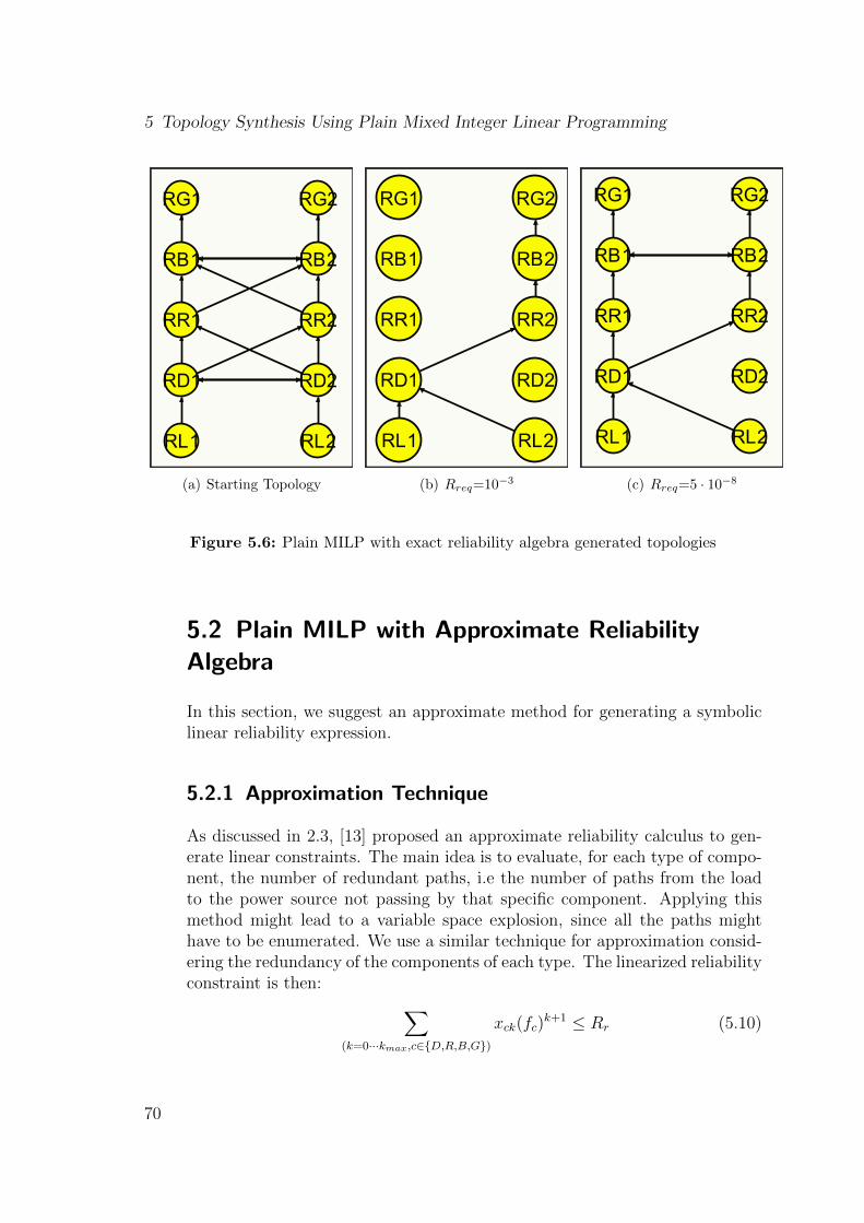
5 Topology Synthesis Using Plain Mixed Integer Linear Programming
RG1 RG2
RB1 RB2
RR1 RR2
RD1 RD2
RL1 RL2
(a) Starting Topology
RG1 RG2
RB1 RB2
RR1 RR2
RD1 RD2
RL1 RL2
(b) Rreq=10−3
RG1 RG2
RB1 RB2
RR1 RR2
RD1 RD2
RL1 RL2
(c) Rreq=5 · 10−8
Figure 5.6: Plain MILP with exact reliability algebra generated topologies
5.2 Plain MILP with Approximate ReliabilityAlgebra
In this section, we suggest an approximate method for generating a symboliclinear reliability expression.
5.2.1 Approximation Technique
As discussed in 2.3, [13] proposed an approximate reliability calculus to gen-erate linear constraints. The main idea is to evaluate, for each type of compo-nent, the number of redundant paths, i.e the number of paths from the loadto the power source not passing by that specific component. Applying thismethod might lead to a variable space explosion, since all the paths mighthave to be enumerated. We use a similar technique for approximation consid-ering the redundancy of the components of each type. The linearized reliabilityconstraint is then: ∑
(k=0···kmax,c∈{D,R,B,G})
xck(fc)k+1 ≤ Rr (5.10)
70
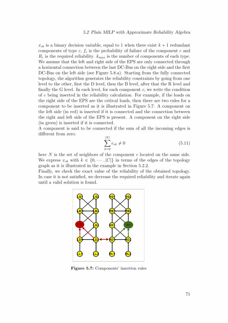
5.2 Plain MILP with Approximate Reliability Algebra
xck is a binary decision variable, equal to 1 when there exist k + 1 redundantcomponents of type c, fc is the probability of failure of the component c andRr is the required reliability. kmax is the number of components of each type.We assume that the left and right side of the EPS are only connected througha horizontal connection between the last DC-Bus on the right side and the firstDC-Bus on the left side (see Figure 5.8.a). Starting from the fully connectedtopology, the algorithm generates the reliability constraints by going from onelevel to the other, first the D level, then the B level, after that the R level andfinally the G level. In each level, for each component c, we write the conditionof c being inserted in the reliability calculation. For example, if the loads onthe right side of the EPS are the critical loads, then there are two rules for acomponent to be inserted as it is illustrated in Figure 5.7: A component onthe left side (in red) is inserted if it is connected and the connection betweenthe right and left side of the EPS is present. A component on the right side(in green) is inserted if it is connected.A component is said to be connected if the sum of all the incoming edges isdifferent from zero:
|N |∑k=0
eck 6= 0 (5.11)
here N is the set of neighbors of the component c located on the same side.We express xck with k ∈ {0, · · · , |C|} in terms of the edges of the topologygraph as it is illustrated in the example in Section 5.2.2.Finally, we check the exact value of the reliability of the obtained topology.In case it is not satisfied, we decrease the required reliability and iterate againuntil a valid solution is found.
Figure 5.7: Components’ insertion rules
71
5 Topology Synthesis Using Plain Mixed Integer Linear Programming
5.2.2 Example of Approximate Reliability ConstraintGeneration
We consider the template in Figure 5.8.a and a reliability requirement Rreq
equal to 10−9. We suppose that the critical loads are the loads on the rightside of the EPS. In this example, the variable level contains a list of the com-ponents of the same type.
DC-Bus levellevel={RD1, RD2, LD1, LD2}Decision variables={eRD2,RD1,eRD1,LD2,eLD2,LD1}The probability of failure in the DC-Bus level is:RD = xD 0fD + xD 1f
2 + xD 2f3 + xD 3f
4
xD 0 = 1⇔ eRD2,RD1 + eRD1,LD2 + eLD2,LD1 = 0xD 1 = 1⇔ eRD2,RD1 + eRD1,LD2 + eLD2,LD1 = 1xD 2 = 1⇔ eRD2,RD1 + eRD1,LD2 + eLD2,LD1 = 2xD 3 = 1⇔ eRD2,RD1 + eRD1,LD2 + eLD2,LD1 = 3The product and the disjunction of the decision variables are linearized asdiscussed in section 5.1.2.
Rectifier levellevel={RR1, RR2, LR1, LR2}RR1 is inserted ⇔ xRR1 = eRD2,RR1 ∨ eRD1,RR1 = 1RR2 is inserted ⇔ xRR2 = eRD2,RR2 ∨ eRD1,RR2 = 1LR1 is inserted ⇔ xLR1 = (eLD2,LR1 ∨ eLD1,LR1) ∧ eLD1,RD2 = 1LR2 is inserted ⇔ xLR2(eLD2,LR2 ∨ eLD1,LR2) ∧ eLD1,RD2 = 1The probability of failure in the rectifier level is:RR = xR 0fR + xR 1f
2R + xR 2f
3R + xR 3f
4R
xR 0 = 1⇔ xRR1 + xRR2 + xLR1 + xLR2 = 1xR 1 = 1⇔ xRR1 + xRR2 + xLR1 + xLR2 = 2xR 2 = 1⇔ xRR1 + xRR2 + xLR1 + xLR2 = 3xR 3 = 1⇔ xRR1 + xRR2 + xLR1 + xLR2 = 4
AC-Bus levellevel={RB1, RB2, LB1, LB2}RB1 is inserted ⇔ xRB1 = eRR2,RB1 ∨ eRR1,RB1 = 1RB2 is inserted ⇔ xRB2 = eRR2,RB2 ∨ eRR1,RB2 = 1LB1 is inserted ⇔ xLB1 = (eLR2,LB1 ∨ eLR1,LB1) ∧ eLR1,RR2 = 1LB2 is inserted ⇔ xLB2(eLR2,LB2 ∨ eLR1,LB2) ∧ eLR1,RR2 = 1The probability of failure in the AC-Bus level is:RB = xB 0fB + xB 1f
2B + xB 2f
3 + xB 3f4B
xB 0 = 1⇔ xRB1 + xRB2 + xLB1 + xLB2 = 1
72
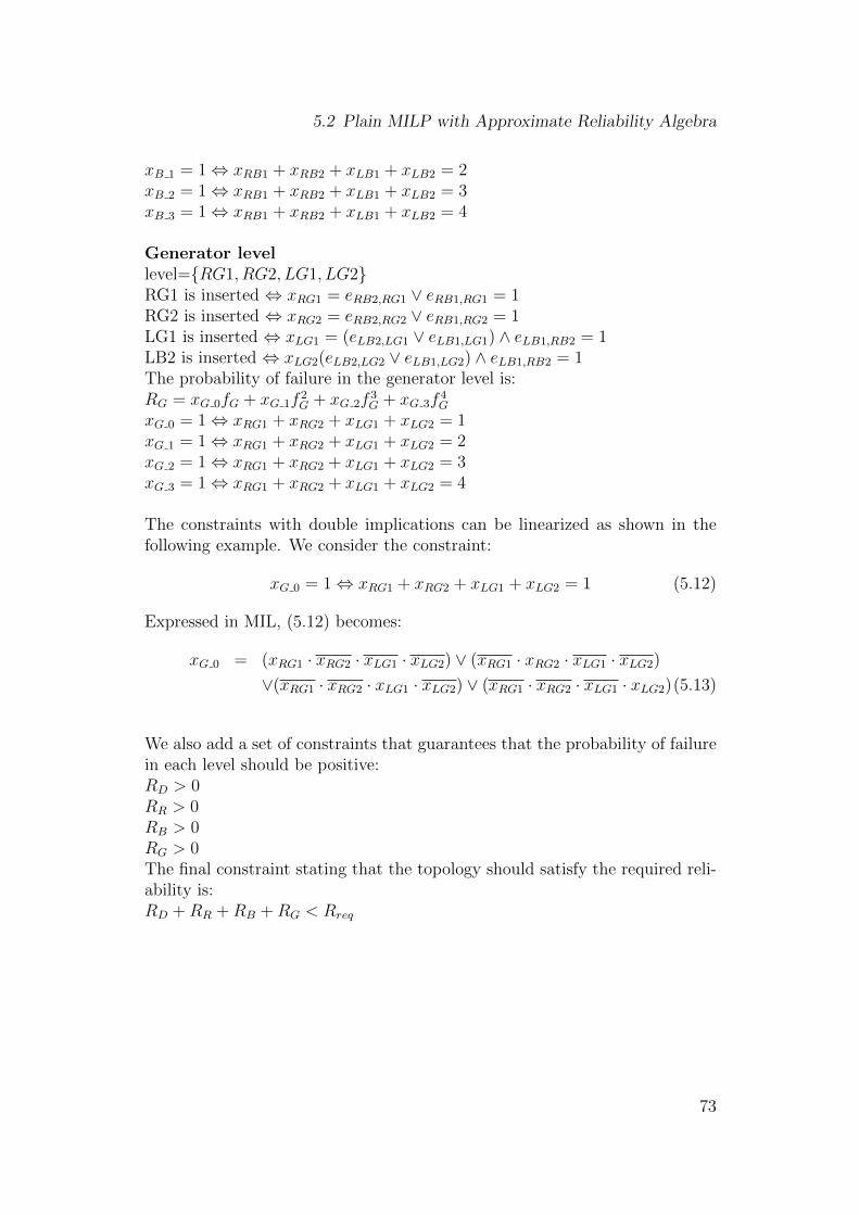
5.2 Plain MILP with Approximate Reliability Algebra
xB 1 = 1⇔ xRB1 + xRB2 + xLB1 + xLB2 = 2xB 2 = 1⇔ xRB1 + xRB2 + xLB1 + xLB2 = 3xB 3 = 1⇔ xRB1 + xRB2 + xLB1 + xLB2 = 4
Generator levellevel={RG1, RG2, LG1, LG2}RG1 is inserted ⇔ xRG1 = eRB2,RG1 ∨ eRB1,RG1 = 1RG2 is inserted ⇔ xRG2 = eRB2,RG2 ∨ eRB1,RG2 = 1LG1 is inserted ⇔ xLG1 = (eLB2,LG1 ∨ eLB1,LG1) ∧ eLB1,RB2 = 1LB2 is inserted ⇔ xLG2(eLB2,LG2 ∨ eLB1,LG2) ∧ eLB1,RB2 = 1The probability of failure in the generator level is:RG = xG 0fG + xG 1f
2G + xG 2f
3G + xG 3f
4G
xG 0 = 1⇔ xRG1 + xRG2 + xLG1 + xLG2 = 1xG 1 = 1⇔ xRG1 + xRG2 + xLG1 + xLG2 = 2xG 2 = 1⇔ xRG1 + xRG2 + xLG1 + xLG2 = 3xG 3 = 1⇔ xRG1 + xRG2 + xLG1 + xLG2 = 4
The constraints with double implications can be linearized as shown in thefollowing example. We consider the constraint:
xG 0 = 1⇔ xRG1 + xRG2 + xLG1 + xLG2 = 1 (5.12)
Expressed in MIL, (5.12) becomes:
xG 0 = (xRG1 · xRG2 · xLG1 · xLG2) ∨ (xRG1 · xRG2 · xLG1 · xLG2)
∨(xRG1 · xRG2 · xLG1 · xLG2) ∨ (xRG1 · xRG2 · xLG1 · xLG2)(5.13)
We also add a set of constraints that guarantees that the probability of failurein each level should be positive:RD > 0RR > 0RB > 0RG > 0The final constraint stating that the topology should satisfy the required reli-ability is:RD +RR +RB +RG < Rreq
73
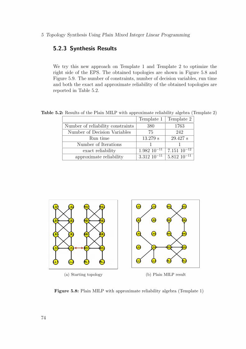
5 Topology Synthesis Using Plain Mixed Integer Linear Programming
5.2.3 Synthesis Results
We try this new approach on Template 1 and Template 2 to optimize theright side of the EPS. The obtained topologies are shown in Figure 5.8 andFigure 5.9. The number of constraints, number of decision variables, run timeand both the exact and approximate reliability of the obtained topologies arereported in Table 5.2.
Table 5.2: Results of the Plain MILP with approximate reliability algebra (Template 2)
Template 1 Template 2
Number of reliability constraints 380 1763Number of Decision Variables 75 242
Run time 13.279 s 29.427 sNumber of Iterations 1 1
exact reliability 1.982 10−11 7.151 10−12
approximate reliability 3.312 10−11 5.812 10−11
(a) Starting topology
RG1 RG2
RB1 RB2
RR1 RR2
RD1 RD2
RL1 RL2
LG1 LG2
LB1 LB2
LR1 LR2
LD1 LD2
LL1 LL2
(b) Plain MILP result
Figure 5.8: Plain MILP with approximate reliability algebra (Template 1)
74
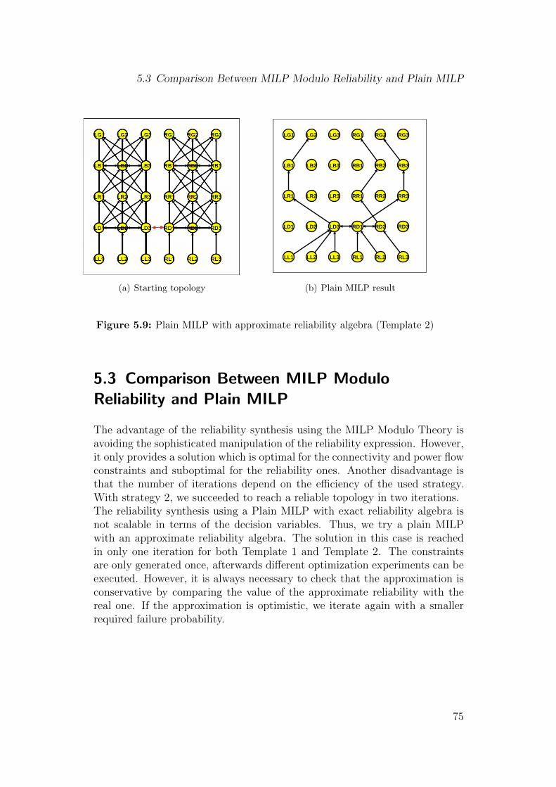
5.3 Comparison Between MILP Modulo Reliability and Plain MILP
(a) Starting topology
RG1 RG2 RG3
RB1 RB2 RB3
RR1 RR2 RR3
RD1 RD2 RD3
RL1 RL2 RL3
LG1 LG2 LG3
LB1 LB2 LB3
LR1 LR2 LR3
LD1 LD2 LD3
LL1 LL2 LL3
(b) Plain MILP result
Figure 5.9: Plain MILP with approximate reliability algebra (Template 2)
5.3 Comparison Between MILP ModuloReliability and Plain MILP
The advantage of the reliability synthesis using the MILP Modulo Theory isavoiding the sophisticated manipulation of the reliability expression. However,it only provides a solution which is optimal for the connectivity and power flowconstraints and suboptimal for the reliability ones. Another disadvantage isthat the number of iterations depend on the efficiency of the used strategy.With strategy 2, we succeeded to reach a reliable topology in two iterations.The reliability synthesis using a Plain MILP with exact reliability algebra isnot scalable in terms of the decision variables. Thus, we try a plain MILPwith an approximate reliability algebra. The solution in this case is reachedin only one iteration for both Template 1 and Template 2. The constraintsare only generated once, afterwards different optimization experiments can beexecuted. However, it is always necessary to check that the approximation isconservative by comparing the value of the approximate reliability with thereal one. If the approximation is optimistic, we iterate again with a smallerrequired failure probability.
75

5 Topology Synthesis Using Plain Mixed Integer Linear Programming
Table 5.3: Comparison between Plain MILP and MILP Modulo Reliability
Plain MILP Plain MILP MILPMR MILPMR(Template 1) (Template 2) (Template 1) (Template 2)
Number of Iterations 1 1 2 2Run time 7.8 s 14.1649 s 14.695 s 19.770 s
76
6 Conclusions and Future Work
In this thesis, we introduce two methodologies to algorithmically synthesizecyber-physical architectural models for an aircraft electrical power distribu-tion system (EPS). The first approach is denoted as a Mixed Integer LinearProgramming Modulo Reliability. A MILP solver is placed in a loop witha reliability analysis tool that evaluates the reliability of the EPS topologygenerated only by solving the power flow and connectivity constraints. If theobtained topology does not satisfy the required reliability, new connectivityconstraints are added to force more redundancy in the architecture. Thisprocess is iteratively repeated until a topology with the desired reliability isreached. Although this approach is advantageous, since it avoids the sophisti-cated manipulation of the reliability expressions, it only provides a suboptimalsolution for the reliability constraints. Besides, its efficiency (the number ofiterations) highly depends on the efficiency of the used strategy.To obtain an optimal topology for all the constraints in only one iteration,we have proposed a Plain MILP methodology based on generating the sym-bolic expression of the reliability constraints. The reliability expression issynthesized from a reconfigurable topology template, linearized and then useddirectly in the MILP solver. The results of the Plain MILP with an exactreliability algebra show that this method poorly scales with the number ofcomponents. We then propose a Plain MILP using an approximate reliabil-ity algebra to synthesize an approximate symbolic expression of the reliabilitybased on the redundancy of the components of each type. This approach suc-cessfully generates a reliable topology in only one iteration.In the future, the proposed synthesis methods will be applied to other sys-tems, such as communication networks, for efficient design of reconfigurablearchitectures subject to reliability constraints.
77

Bibliography
[1] C. Lucet and J.-F. Manouvrier, “Exact methods to compute networkreliability,” in Statistical and Probabilistic Models in Reliability, ser.Statistics for Industry and Technology, D. Ionescu and N. Limnios,Eds. Birkhuser Boston, 1999, pp. 279–294. [Online]. Available:http://dx.doi.org/10.1007/978-1-4612-1782-4 20
[2] [Online]. Available: http://gerard-avontuur.tripod.com/Chapter2/Chapter2.html
[3] L. Guo, M. Maasoumy, M. Mozumdar, P. Nuzzo, N. Ozay, U. Topcu,et al., “Aircraft electric power system: Description, Specifications andDesign Challenges,” Tech. Rep.
[4] [Online]. Available: https://chess.eecs.berkeley.edu/design/2012/lectures/EE249 3 ThePlatformConcept.pdf
[5] P. Nuzzo, “A contract based methodology for aircraft electrical power sys-tem,” EECS Department, University of California Berkeley, Tech. Rep.,2012.
[6] R. Brayton and J. Cong, “Electronic design automation past, present,and future,” NSF, Tech. Rep., 2009.
[7] A. Sangiovanni-Vincentelli, “Quo vadis, SLD? reasoning about the trendsand challenges of system level design,” Proceedings of the IEEE, vol. 95,no. 3, pp. 467–506, 2007.
[8] S. Rai and K. Aggarwal, “An efficient method for reliability evaluation ofa general network,” Reliability, IEEE Transactions on, vol. R-27, no. 3,pp. 206–211, 1978.
[9] Y. Shen, “A new simple algorithm for enumerating all minimal pathsand cuts of a graph,” Microelectronics Reliability, vol. 35, no. 6, pp. 973– 976, 1995. [Online]. Available: http://www.sciencedirect.com/science/article/pii/0026271494001214
[10] A. K. Verma, S. Ajit, and D. R. Karanki, Reliability and Safety engineer-ing. Springer, 2010.
79
Bibliography
[11] B. Kaiser, P. Liggesmeyer, and O. Mackel, “A new component conceptfor fault trees,” in Proceedings of the 8th Australian workshop on Safetycritical systems and software - Volume 33, ser. SCS ’03. Darlinghurst,Australia, Australia: Australian Computer Society, Inc., 2003, pp. 37–46.[Online]. Available: http://dl.acm.org/citation.cfm?id=1082051.1082054
[12] B. Kaiser and A. Zocher, “BDD complexity reduction by component faulttrees,” Proceedings of the the European Safety and Reliability Conference.
[13] P. Helle, M. Masin, and L. Greenberg, “Approximate reliabilityalgebra for architecture optimization,” in Proceedings of the 31stinternational conference on Computer Safety, Reliability, and Security,ser. SAFECOMP’12, 2012, pp. 279–290. [Online]. Available: http://dx.doi.org/10.1007/978-3-642-33678-2 24
[14] A. Pinto, S. Becz, and H. M. Reeve, “Correct-by-construction design ofaircraft electric power systems,” in 2010 AIAA ATIO/ISSMO Conference,September 2010.
[15] P. Manolios and V. Papavasileiou, “ILP modulo theories,” CoRR, vol.abs/1210.3761, 2012.
[16] S. Jha, R. Limaye, and S. Seshia, Beaver: Engineering anEfficient SMT Solver for Bit-Vector Arithmetic, ser. Lecture Notesin Computer Science, A. Bouajjani and O. Maler, Eds. SpringerBerlin Heidelberg, 2009, vol. 5643. [Online]. Available: http://dx.doi.org/10.1007/978-3-642-02658-4 53
[17] [Online]. Available: http://users.isy.liu.se/johanl/yalmip/
[18] [Online]. Available: http://www-01.ibm.com/software/commerce/optimization/cplex-optimizer/
80

Confirmation
Herewith I confirm that I independently prepared this work. No further ref-erences or auxiliary means except those declared in this document have beenused.
Munich, June 11, 2013
. . . . . . . . . . . . . . . . . . . .
Safa Messaoud
View publication statsView publication stats