Embed Size (px)
Citation preview
1
Optimal Pixel Aspect Ratio for Enhanced 3D TV Visualization
Hossein Azari1, Irene Cheng
1, Kostas Daniilidis
2 and Anup Basu
1
1Department of Computing Science, University of Alberta, Edmonton, Alberta, Canada
2Dept. of Computer and Information Science, University of Pennsylvania, Philadelphia, USA
EMAIL: [email protected], [email protected], [email protected] and [email protected]
Phone: 780-492-3330, FAX: 780-492-1071
Parts of this work have been presented at the IEEE 3D TV Conference, Istanbul, Turkey, 2008.
2
ABSTRACT
In multiview 3D TV, a pair of corresponding pixels in adjacent 2D views contributes to the
reconstruction of voxels (3D pixels) in the 3D scene. We analyze this reconstruction process and
determine the optimal pixel aspect ratio based on which the estimated object position can be improved
given specific imaging or viewing configurations and constraints. By applying mathematical modeling,
we deduce the optimal solutions for two general stereo configurations: parallel and with vergence. We
theoretically show that a non-uniform finer horizontal resolution, compared to the usual uniform pixel
distribution, in general provides a better 3D visual experience for both configurations. The optimal value
may vary depending on different configuration parameter values. We validate our theoretical results by
conducting subjective studies using a set of simulated non-uniformly discretized red-blue stereo pairs and
show that human observers indeed have a better 3D viewing experience with an optimized vs. a non-
optimized representation of 3D-models.
Keywords: Aspect ratio, vergence, 3D TV, perceptual quality, sense of depth, stereo display

3
1. INTRODUCTION
Over the past few years, 3D TV technologies have received increasing public attention with wide
applications in IMAX and entertainment centres. Research in this area covers issues relating to 3D video
capture, transmission, and display [1],[2],[3],[4],[5]. Extensive research has also been conducted on
designing 3D displays including studies on display screen aspect ratio [6]. These studies show that screen
dimension with width:height ratios between 5:3 and 6:3 are more visually pleasant to the viewers [7]. In
this regard, wider displays provide a better sensation of depth even with 2D images. This observations
have led to designing wider screens for HDTV displays compared to previous generation TVs [6].
Different from the screen aspect ratio, a square pixel component with an aspect ratio of 1:1 is usually
adopted by 2D digital media devices, although research suggested that non-uniform pixel aspect ratios
can create better visual experience [9]. Despite this observation, there is not much work addressing the
problem of determining an appropriate aspect ratio of pixels with respect to the parameters affecting the
3D picture formation process on (auto)stereoscopic displays. By default, similar to conventional 2D
displays, square pixels have been adopted to compose different views of 3D displays; whereas, such an
arbitrary decision may not be consistent with the underlying depth perception inherent in the human
visual system.
Differing from conventional 2D displays, the output of a stereoscopic 3D display is constructed based
on two or more different views of the same scene. That is, the 3D points of the reconstructed virtual 3D
scene are computed based on the corresponding pixels of adjacent 2D views. Since discrete pixels are
involved in 3D point reconstruction, discretization error [8], [9], [10] is expected in the 3D point
estimation process. The magnitude of this error depends on the inter-pixel distance in the 2D views and
the viewing distance. For 3D displays, discretization is closely related to the 3D resolution or stereoscopic
resolution which is defined in terms of the precision in locating 3D points within the comfortable viewing
range of the 3D display [11]. The magnitude of this error depends on the inter-pixel distance in the 2D
views and is proportional to the viewing distance. In other words, the discretization error, or equivalently

4
stereoscopic resolution on each 3D coordinate component (horizontal, vertical, and depth resolution), is
directly related to the size of pixels; and depending on the stereo configuration parameters the relative
width and height of a pixel can affect the amount of these errors differently. Since the horizontal and
vertical discretizations contribute separately to the 3D point estimation error, given a total display
resolution the challenge is to compute an optimal horizontal vs. vertical discretization in a unit area (pixel
aspect ratio) that can minimize the error, in order to maximize the 3D-display viewing quality without
changing the total resolution. This optimization issue is important especially for multi-view 3D displays,
which provide several different 3D views (currently 6-9 views) and require several 2D images as input (7-
10 images for 6-9 3D views).
In this paper, we study the abovementioned optimization problem for different stereo configurations.
We extend our earlier research [8, 9, 10, 12, 13] and conduct subjective studies using two stereo
configurations: parallel and with vergence. We show that the aspect ratio of pixels for optimizing 3D
reconstruction can vary significantly in different configurations. Moreover, based on the physical pixel
grouping technique, we present methods that simulate 3D viewing with different pixel aspect ratios on
conventional 2D displays. These methods enable us to conduct human observer evaluations on both
simple and complex 3D objects. Our evaluation results, which are consistent with our theoretical
derivations, show that given a constant total resolution it is possible to improve the 3D visual experience
by choosing a finer horizontal resolution relative to the vertical display resolution. The optimal value may
vary depending on the parameter settings. In our implementation, we follow the usual viewing conditions
to specify these parameters.
The remainder of this paper is organized as follows: Section 2 formally defines the problem and
notation used in this paper. Section 3 discusses optimal discretization for a single 3D point with and
without vergence. Results obtained in Section 3 are extended in Section 4 to determine the optimal aspect
ratio within the viewing volume inside a camera’s field of view. Experimental results and subjective
studies are described in detail in Section 5. Finally, concluding remarks and suggestions for future work
are outlined in Section 6.
5
2. PROBLEM DEFINITION AND NOTATION
We use the same notation and definitions as in our earlier publications (see Figures 1 and 2):
f: focal length of both cameras.
),,( ZYX : a 3D point, and )ˆ,ˆ,ˆ( ZYX : estimated 3D position.
(xl, yl): projection of a 3D point on the left image.
(xr, yr): projection of a 3D point on the right image.
ex (ey): distance between two neighboring pixels (picture elements or viewing elements) in the x (y)
direction.
bx: baseline of a stereo imaging setup.
R: total resolution, i.e., the total number of pixels or viewing elements being used for stereo capture
or viewing.
Using triangulation rules, the image projections of a 3D point on the left and right image screens in
parallel geometry (Figure 1) are given by:
Z
fYyyy
Z
bXfx
Z
fXx rl
xlr
,
)(, ( 1 )
Thus, a 3D point location ),,( ZYX can be computed as:
Figure 1: Left: parallel-camera stereo projection with baseline bx. Right: discretization error.
Left Image
Right Image
(X,Y,Z)
Z
X Y
(0,0,0)
(bx,0,0)
(xl ,y)
(xr ,y)
Pixel:
ex
ey
(xl ,y)
Left image pixels
)ˆ,ˆ( yxl

6
lr
xr
xx
fbZ
f
yZY
f
xZX
,, ( 2 )
In practice, since the image projections are discretized to the nearest pixel, location of a 3D-point is
determined using points )ˆ,ˆ( yxr and )ˆ,ˆ( yxl . Therefore, the location of a 3D-point (X,Y,Z) is estimated as:
lr
xr
xx
fbZ
f
yZY
f
xZX
ˆˆˆ,
ˆˆˆ,ˆˆˆ
( 3 )
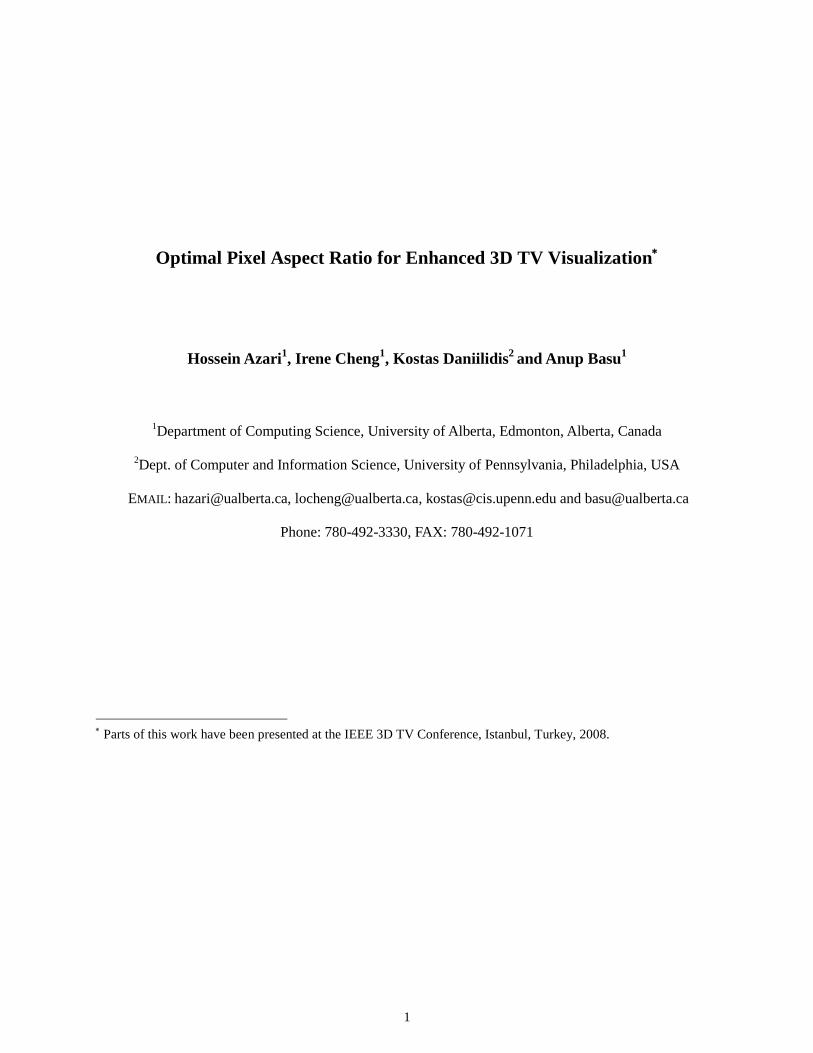
For cameras with vergence (Figure 2), the location of a 3D point ),,( ZYX can be computed using
following formulae (see [10] for details):
)sincos)(cossin()cossin)(sincos(
)sincos)(sincos(
)cossin(
)sincos(
)cossin(
rlrl
rlx
r
r
r
xfxfxfxf
xfxfbZ
f
ZXyY
xf
xfZX
( 4 )
Again, because of discretization error )ˆ,ˆ( rr yx and )ˆ,ˆ( ll yx will be used in the computations resulting in an
estimation error with respect to the original 3D point.
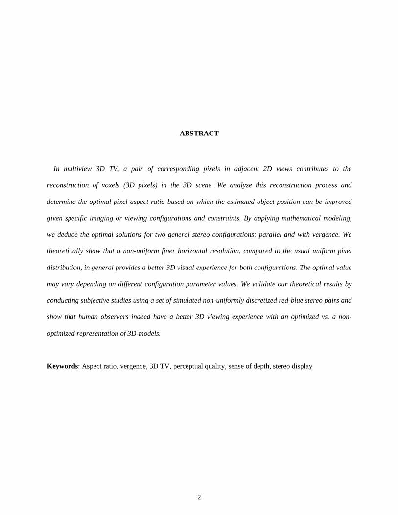
Figure 3 shows the error pattern for two camera configurations (left: parallel geometry and middle:
vergence geometry). Figure 3 (right) illustrates a 3D-view of an error generated by two corresponding
pixels. The quadrilateral volume corresponds to a voxel (3D pixel). Obviously, reducing the pixel size and
thus increasing the total resolution will reduce the voxel size as well as the 3D point estimation error.
Left Image
Right Image
(X,Y,Z)
Z
Y
(0,0,0)
(bx,0,0)
ZL
ZR α
α
XL
XR
X
(xl , yl)
(xr , yr)
Pixel:
ex
ey
(xl ,yl)
)ˆ,ˆ( ll yx
Left image pixels
Figure 2: Left: Stereo camera projection with vergence and baseline bx. Right: discretization error.

7
However, assuming a constant total resolution R, it is reasonable to look for an optimal pixel aspect ratio
which minimizes the size of voxels or equivalently the discretization error inside the viewing region. Such
optimization can improve the output image quality of a typical 3D TV system while the size of the input
data is unchanged. The optimal solution can also be used in solving the stereo based depth estimation
problem, which has been a research focus in the past decades [14], [15].
3. OPTIMAL DISCRETIZATION FOR A SINGLE 3D POINT ESTIMATION
As mentioned in the previous section, the discrete nature of a display device (or viewing screen) leads to
rounding. The rounding error is bounded by half a pixel. Thus, in the worst case:
)2/(ˆˆˆ
)2/(ˆ
)2/(ˆ
ylr
xll
xrr
eyyyy
exx
exx
( 5 )
Considering the stereo setup with parallel configuration (shown in Figure 1), and the worst-case error in
3D estimation, which will be our default assumption in the rest of this paper, we obtain Z from Equations
3 and 5 (as explained in [8]):
1
1)(
ˆ
x
x
xlr
x
fb
ZeZ
exx
fbZ ( 6 )
The Taylor series expansion of Equation 6 about Z = 0 is given by:
3
3
2
21
11ˆ Zfb
eZ
fb
eZ
fb
eZ
fb
ZeZZ
x
x
x
x
x
x
x
x
Figure 3: Discretization error patterns. Left: parallel-axes stereo. Middle: stereo with vergence. Right: 3D-view of
error pattern for two corresponding pixels.
)ˆ,ˆ,ˆ( ZYX
Right pixel
Corresponding left pixel

8
In practice f and bx values are much greater than values taken by ex. Therefore, we can assume that the
higher order terms in the above expansion are negligible. As result, Z can be properly approximated as:
x
x
fb
ZeZZ 1ˆ ( 7 )
Bounds on error in estimating X can be obtained as follow:
rx
x
r
x
x
x
xr
x
xr
xfb
Ze
x
e
fb
ZeX
ex
fb
Ze
f
Zx
f
ZX
221
21ˆ
ˆˆ
2
( 8 )
Similarly, for Y:
yfb
Zee
y
e
fb
ZeYY
x
yxy
x
x
221ˆ
or,
x
yxy
x
xyxp
byf
Zee
y
e
fb
Zeeef
Y
YY
22),(
ˆ ( 9 )
Considering a unit viewing or image capture area:
Re
eRee x
y
yx
1or
11
( 10 )
From Equations 9 and 10 we have:
xx
x
x
xpRbyf
Z
eyRe
fb
Zef
2
1
2
1)( ( 11 )
From Equation 8 it is obvious that the best solution which minimizes the estimation error of X or Z is to
have ex as small as possible. Unfortunately, it is also the worst possible choice for estimating the Y
component. As a compromise, Equation 11, which is the upper bound of the relative estimation error in Y
as a function of ex constrained by the total resolution R through Equation 10, can be used to find the best
vertical vs. horizontal resolution tradeoff for estimating Y. The advantage of using relative versus absolute
estimation error in the optimization process is to offset the monotonic increase of absolute error in the
vertical direction from the center of the image plane, and allows the discretization optimization problem

9
to be studied independent of the pixel location on the image plane. Our analysis motivates the derivations
of a Mathematical model given below.
Result 1 – Optimal discretization for a single 3D point and parallel configuration: Considering the
parallel stereo configuration in Figure 1, the optimal discretization for estimating Y for a single 3D point
is:
x
y
x
xfb
Zy
Re
Zy
fb
Re
21 ,
2
1 ( 12 )
Derivation: The results are obtained by equating the derivative of fp(ex) in Equation 11 to zero to
minimize the error:
02
11)(
2
yRefb
Zef
xx
xp ( 13 )
Solving Equation 13
in terms of
ex gives the value of ex in Equation
12. To show that the function fp
achieves the minimum value at this point we need to perform the second derivative test. From Equation
13 the second derivative of fp in terms of ex is calculated as:
3
11)(
x
xpeyR
ef
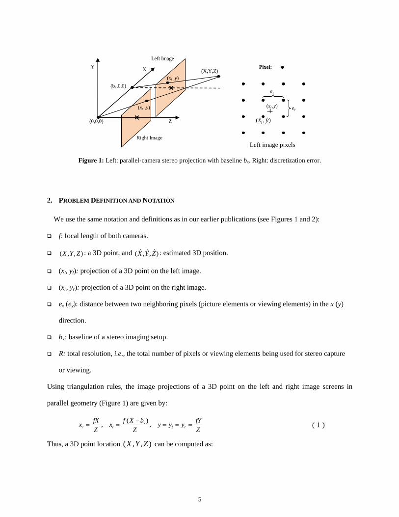
Figure 4: Comparing discretization error pattern and changes of error in estimation of Y for regular square pixels,
ex = ey, (left) vs. vertically rectangular pixels, ex < ey, with optimal pixel aspect ratio (right).
Decrease of maximum error
in estimation of Y
Corresponding
right pixel
Left pixel
)ˆ,ˆ,ˆ( ZYX
Left pixel
)ˆ,ˆ,ˆ( ZYX
Corresponding
right pixel
Increase of error in estimation
of Y for some other 3D points

10
On the other hand, from Equation 10 we can see that ex changes over the open interval (0,∞) which means
that ex always takes positive values. Since the other two parameters involved in the above equation are
also positive, the second derivative of fp is always positive over the domain of possible values for ex. As a
result, fp is strongly convex over this domain and takes its minimum value at ex given by Equation 12. The
value of ey in Equation 12 can be obtained from ex by applying Equation 10.
The solution that is obtained in this way is not only optimal in terms of the maximum relative estimation
error on Y, but often yields better estimates for the X and Z components as well. From 12 the ratio of ex to
ey can be calculated as:
y
xx
Zy
fb
e
e lrx
y
x
2
)(
2
( 14 )
In Equation 14, (xr – xl) is the amount of the disparity between the corresponding points in the left and
right image planes. It should be clarified that xr and xl in above-mentioned equations are measured with
respect to the corresponding camera coordinate system. As result, and as can be also deducted from
Equation 2, (xr – xl) is always greater than or equal to zero.
The amount of disparity (xr – xl) in most (practical) cases is smaller than 2|y|. This means that in
practice the ratio in Equation 14 is usually less than one or equivalently ex is often smaller than ey. As a
result, the optimal solution in Result 1 often improves the estimates of the X and Z components. However,
when ex < ey the optimal solution changes the error pattern so that the Y estimation error may be increased
for some 3D points estimated by )ˆ,ˆ,ˆ( ZYX . This phenomenon is pictorially illustrated in Figure 4 for a
typical error pattern. As shown in Figure 4, the optimal pixel aspect ratio less than one (i.e. ex < ey) results
in improvement in estimation of X and Z plus reduction of the maximum error in estimation of Y, which
in turn means improvement of estimation of Y for some 3D points. But generally this is achieved in the
cost of degradation in the estimation of Y for some other 3D points.
11
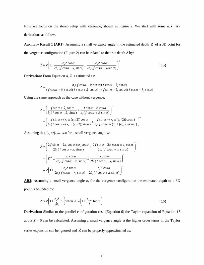
Now we focus on the stereo setup with vergence, shown in Figure 2. We start with some auxiliary
derivations as follow.
Auxiliary Result 1 (AR1): Assuming a small vergence angle α, the estimated depth Z of a 3D point for
the vergence configuration (Figure 2) can be related to the true depth Z by:
1
)sincos(2
cos
)sincos(2
cos1ˆ
lx
x
rx
x
xfb
Ze
xfb
ZeZZ ( 15 )
Derivation: From Equation 4, Z is estimated as:
)sinˆcos)(cosˆsin()cosˆsin)(sinˆcos(
)sinˆcos)(sinˆcos(ˆ
rlrl
rlx
xfxfxfxf
xfxfbZ
Using the same approach as the case without vergence:
1
1
)sin))2((cos(
)cos))2((sin
)sin))2((cos(
cos))2((sin
)sinˆcos(
cosˆsin
)sinˆcos(
cosˆsinˆ
xlx
xl
xrx
xr
lx
l
rx
r
exfb
exf
exfb
exf
xfb
xf
xfb
xfZ
Assuming that 0sin2 xe for a small vergence angle :
1
1
1
1
)sincos(2
cos
)sincos(2
cos1
)sincos(2
cos
)sincos(2
cos
)sincos(2
coscos2sin2
)sincos(2
coscos2sin2ˆ
lx
x
rx
x
lx
x
rx
x
lx
xl
rx
xr
xfb
Ze
xfb
ZeZ
xfb
e
xfb
eZ
xfb
exf
xfb
exfZ
AR2: Assuming a small vergence angle α, for the vergence configuration the estimated depth of a 3D
point is bounded by:
tan1 where1ˆ max
f
xKK
fb
ZeZZ
x
x ( 16 )
Derivation: Similar to the parallel configuration case (Equation 6) the Taylor expansion of Equation 15
about Z = 0 can be calculated. Assuming a small vergence angle the higher order terms in the Taylor
series expansion can be ignored and Z can be properly approximated as:

12
)sincos(
cos
2)sincos(
cos
21ˆ
lx
x
rx
x
xfb
Ze
xfb
ZeZZ ( 17 )
Expanding the second term of Equation 17 and ignoring higher order terms, we have:
tan1
1
cos
sin1
1
)sincos(
cos1
f
x
ff
x
fxf
rr
r
( 18 )
Similarly, for the third term:
tan1
1
cos
sin1
1
)sincos(
cos1
f
x
ff
x
fxf
ll
l
( 19 )
From Equations 17, 18, and 19:
tan11
tan)(
22
1
tan11
2tan1
1
21ˆ
max
f
x
fb
ZeZ
f
xx
fb
ZeZ
f
x
fb
Ze
f
x
fb
ZeZZ
x
x
lr
x
x
l
x
xr
x
x
( 20 )
where
2maxmax
lr xxx is half of the maximum possible horizontal disparity, which is in fact equal to
the maximum possible value of x or equivalently half of the image plane (or display) width.
AR3: Assuming a small vergence angle α:
xrxr
x
x
xvRbyf
ZK
eyRe
fb
ZKef
Y
YY
2
1
2
1)(
ˆ ( 21 )
Derivation: For a small vergence angle , the parallel configuration formulae can be used to approximate
the Y component. Therefore:
lx
yx
r
y
x
x
y
r
x
xr
yfb
ZKee
y
e
fb
ZKeY
eyK
fb
Ze
f
Z
f
yZY
221
21
ˆˆˆ
( 22 )
Considering a total resolution of R, Equation 21 can be obtained from Equations 10 and 22.
13
Summarizing the abovementioned derivations, the following result can be stated for a stereo
configuration with vergence.
Result 2 – Optimal discretization for a single 3D point and stereo setup with vergence: Considering a
stereo system with a small vergence angle (Figure 2), the optimal discretization for a single 3D point
can be obtained as:
x
r
y
r
xx
fb
ZKy
Re
ZKy
fb
Re
21 ,
2
1 ( 23 )
Derivation: Similar to the parallel configuration, from Equation 21:
2
1
2
1)(
xrx
xveyRfb
ZKef
( 24 )
The results can be obtained by equating 24 to zero, and solving it in terms of ex . The same argument as
Result 1 can be applied to show that fv indeed takes its minimum value at this point, considering the
domain of permissible values for ex.
4. OPTIMIZING WITHIN A VIEWING VOLUME
The derivations in the last section consider optimization with respect to a single 3D point. Instead, we
need to consider a region in 3D defined by a set of constraints on the range of values in depth, height and
the stereo Field-Of-View (FOV). Obviously, the particular values obtained for ex (or ey) in the previous
section will not be optimum for all points satisfying these constraints. A solution to this problem could be
calculating the integral of the error function fp or fv over the entire specified region. However, this
approach leads to logarithmic terms which complicate further steps in the optimization process. Instead,
we consider minimizing an appropriate error metric subject to the restrictions imposed.
For the parallel camera configuration (Figure 1), we use Equation 13 to obtain such an error metric. In
this case, from Equation 13 for the optimal discretization ex for a single 3D point we have:

14
ReyZ
fb
yRefb
Z
xx
xx
2
2
2
2
11
or equivalently,
02 2 ReyZ
fbx
x ( 25 )
In other words, for a single 3D point, the derivative of fp or equivalently the right side of Equation 25 is
zero at the optimal discretization and non-zero in its neighbourhood. This, in fact, gives a distance
criterion that can be used as an error metric for optimizing the discretization error over the entire region.
We define the square of this distance as the error metric, as follow:
2
22
Rey
Z
fbE x
xp
( 26 )
On the other hand, for parallel configuration the range of values of X varies with changes of depth Z and
values of the cameras’ field of view by the following simple relationship (see Figure 5-left):
)(
)(
2 0max
00
ZZ
ZZXXX ( 27 )
Thus, we need to optimize the following function w.r.t. ex :
max
min
max
max
0max
00
0max
00
)(
)(
2
)(
)(
2
2
22)(
Z
Z
y
y
ZZ
ZZXX
ZZ
ZZXX
xx
xp dXdydZReyZ
fbeF
( 28 )
Calculating the integral in 28 and equating its derivative to zero gives us the following result:
Result 3 – Optimal discretization for a viewing volume and parallel configuration: Considering the
abovementioned notation and the parallel stereo configuration given in Figure 5-left, and assuming a
reasonably large viewing volume across the Z dimension, the discretization in x for optimizing the
average error in estimation of Y is given by:
2
1
maxmin40maxmin3
maxmin2maxmin10
],[],[
],[],[
2
ZZIZZZI
ZZIZZIZ
R
fbe x
x ( 29 )
where,

15
2
1
max
max1
22
max211 ln],[Z
Z
y
y Z
ZydydZ
Z
yZZI
2
1
max
max
)(],[ 12
2
max212
Z
Z
y
yZZydydZyZZI
2
1
max
max
2
1
2
2
3
max2
2133
],[Z
Z
y
yZZ
ydydZZyZZI
2
1
max
max12
3
max2
2143
2],[
Z
Z
y
yZZ
ydydZyZZI
Derivation: See Appendix A.
Determining the range of values of X when Z varies over a specific domain is a little more complicated
for the vergence configuration (see Figure 5-right). This is because between Z0 to Zint the values of X vary
in a certain way, and for Z > Zint the values of X vary in a different way. The values of Z0 and Zint are
given through the following equations.
AR4: Given a field of view θ and a vergence angle α:
)22
tan(2
0
xb
Z ( 30 )
)2sin(
cos)2cos(
2int
xb
Z ( 31 )
Derivation: Follows from Figures 5 and 6, using simple geometric rules, such as the sine rule. Details are
skipped here.
Figure 5: Viewing region without (left) and with vergence (right).
Zmax
Zmin
Zint
Z0 bx
α
Zmax
Zmin
bx
Z0
02
XX
02
XX
X0

16
AR5: Considering the setup with vergence in Figure 5-right, the range of values of X, depending on depth
Z and the field of view of the cameras, varies based on the following rules:
intint for )2sin(
sin
2ZZ
bX x
( 32 )
int0
0int
0int for
)(
)(ZZZ
ZZ
ZZXX
( 33 )
ZZbZ
ZbXX xx int
int
int for )( ( 34 )
(It is assumed that the X-axis is the dashed line joining the centers’ of the two cameras.)
Derivation: Follows from trigonometric rules and the earlier derivations. Details are skipped here.
Here again, we need to consider an appropriate error metric to minimize over the range of possible X, Y,
and Z values. Similar to the parallel configuration scenario, we use the following error metric based on
the derivative in Equation 24:
2
22
xr
xv RKey
Z
fbE ( 35 )
We thus need to optimize the following function w.r.t. ex (from this point forward, for simplicity we
ignore subscript r in yr):
Z y X
xx
xv dXdydZyRKeZ
fbeF
2
22)( ( 36 )
(/2)+(/2)-
(/2)-(/2)-
2
(/2)-(/2)+
Zint
bx
Figure 6: A close-up of Figure 5 (bottom right) illustrating its geometric constraints.

17
Unlike the multiple integral in Equation 28, the computation of the integral above may need to be divided
into two parts depending on the values of Zmin and Zmax relative to Zint. If Zint ≤ Zmin or Zmax ≤ Zint, we need
to consider either Equation 33 or Equation 34 in computing this integral. However, if Zmin < Zint < Zmax,
then we must consider both Equations 33 and 34.
By calculating Fv(ex) in these three possible cases and equating corresponding derivatives to zero, we
can obtain optimal discretization for all cases (see Appendix A for details). Thus, we can state the
following general result.
Result 4 – Optimal discretization for a viewing volume and stereo setup with vergence: Considering
the abovementioned notation and the stereo system framework in Figure 5-right, and assuming a
reasonably thick viewing volume across the Z dimension, the discretization in x for optimizing the
average error in estimation of Y is given by:
I) Zint ≤ Zmin
2
1
maxmin
maxmin
],[
],[
2
ZZB
ZZA
RK
fbe x
x ( 37 )
II) Zmax ≤ Zint
2
1
maxmin
maxmin
],[
],[
2
ZZD
ZZC
RK
fbe x
x ( 38 )
III) Zmin < Zint < Zmax
2
1
maxintintmin
maxintintmin
],[],[
],[],[
2
ZZDZZB
ZZCZZA
RK
fbe x
x ( 39 )
where,
],[)(
],[],[ 212
int
int21121 ZZI
Z
bXZZIbZZA x
x
],[)(
],[],[ 213
int
int21421 ZZI
Z
bXZZIbZZB x
x
],[],[],[ 211021221 ZZIZZZIZZC
],[],[],[ 214021321 ZZIZZZIZZD
I1 to I4 are equations defined in Result 3.

18
Derivation: See Appendix A.
5. EXPERIMENTAL RESULTS
5.1. NUMERICAL RESULTS
Table 1 shows a typical set of parameter values used for calculating optimal pixel aspect ratios (ex/ey)
for with and without vergence stereo setups. Values of xmax, ymax, and R are set to 3.15 mm, 2 mm and
40635 pixels per mm2, respectively. These values are obtained assuming that a CCD of size 6.3 x 4.0 mm
and a resolution of 1280 x 800 (around 1 mega pixel) is used in the capturing process. Focal length and
stereo baseline are respectively set to 17 and 65 mm, which are close to the human visual system
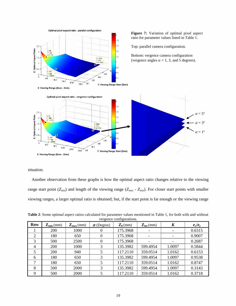
parameters. Table 1 also includes the range of values used for Zmin and Zmax in our calculations. Figure 7
shows the results of our calculations for parameter values in Table 1 based on Result 3 and Result 4 and
other related formulae. Figure 7-left shows how optimal aspect ratio changes with different viewing
volumes at different distances in the parallel configuration. Figure 7-right presents corresponding results
in the vergence configuration using three different small vergence angles, = 1, 3, and 5 degrees, over
the same depth ranges and viewing volumes. The corner of the original graph is magnified in order to
highlight the effect of applying different vergence angles. It can be seen that for small vergence angles
there is no significant difference either between the left and right graphs or between results obtained for
different small vergence angles on the right graph. Based on this observation, we can say that at least for
small vergence angles the effect of vergence in determining the optimal pixel aspect ratio is negligible. It
should be noted that for a stereo baseline of 65 mm, a 5 degree vergence angle is equivalent to focusing
on a point about 371 mm from cameras/viewing point, which is a good representation of a practical
Table 1: Parameters’ values used for calculating optimal pixel aspect ratio.
Parameter Value Parameter Value
f 17 mm Zmin From 200 mm to 600 mm
bx 65 mm Zrange (Zmax- Zmin) From 1 mm to 2000 mm
xmax 3.15 mm Resolution (R) 1280x800 (40635 p/mm2)
ymax 2 mm
19
situation.
Another observation from these graphs is how the optimal aspect ratio changes relative to the viewing
range start point (Zmin) and length of the viewing range (Zmax - Zmin). For closer start points with smaller
viewing ranges, a larger optimal ratio is obtained; but, if the start point is far enough or the viewing range
Table 2: Some optimal aspect ratios calculated for parameter values mentioned in Table 1, for both with and without
vergence configurations.
Row Zmin (mm) Zmax (mm) (Degree) Z0 (mm) Zint (mm) K ex/ey
1 200 1000 0 175.3968 - - 0.6315
2 180 650 0 175.3968 - - 0.9007
3 500 2500 0 175.3968 - - 0.2687
4 200 1000 3 135.3982 599.4954 1.0097 0.5844
5 200 940 5 117.2110 359.0514 1.0162 0.6153
6 180 650 3 135.3982 599.4954 1.0097 0.9538
7 180 650 5 117.2110 359.0514 1.0162 0.8747
8 500 2000 3 135.3982 599.4954 1.0097 0.3143
9 500 2000 5 117.2110 359.0514 1.0162 0.3718
Figure 7: Variation of optimal pixel aspect
ratio for parameter values listed in Table 1.
Top: parallel camera configuration.
Bottom: vergence camera configuration
(vergence angles = 1, 3, and 5 degrees).
= 5
= 3
= 1
20
is large enough, a smaller aspect ratio is obtained. Moreover, from these graphs we can see that even
though the optimal points are obtained by optimization of the relative error in estimating the Y
component, the optimal aspect ratio is smaller than one in most configurations (and in fact in more
practical configurations), which means that the X and Z estimates are improved as well, compared to a
uniform pixel distribution over the x and y axes.
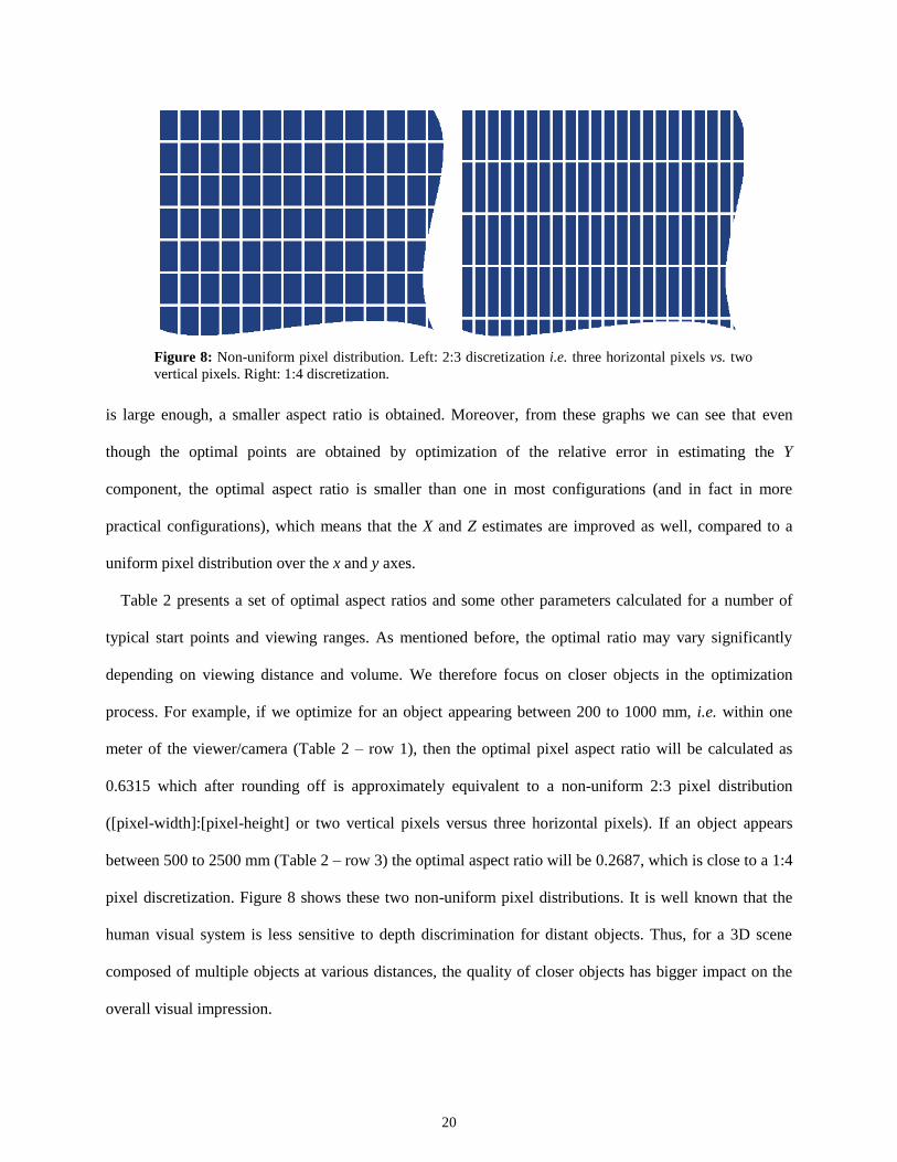
Table 2 presents a set of optimal aspect ratios and some other parameters calculated for a number of
typical start points and viewing ranges. As mentioned before, the optimal ratio may vary significantly
depending on viewing distance and volume. We therefore focus on closer objects in the optimization
process. For example, if we optimize for an object appearing between 200 to 1000 mm, i.e. within one
meter of the viewer/camera (Table 2 – row 1), then the optimal pixel aspect ratio will be calculated as
0.6315 which after rounding off is approximately equivalent to a non-uniform 2:3 pixel distribution
([pixel-width]:[pixel-height] or two vertical pixels versus three horizontal pixels). If an object appears
between 500 to 2500 mm (Table 2 – row 3) the optimal aspect ratio will be 0.2687, which is close to a 1:4
pixel discretization. Figure 8 shows these two non-uniform pixel distributions. It is well known that the
human visual system is less sensitive to depth discrimination for distant objects. Thus, for a 3D scene
composed of multiple objects at various distances, the quality of closer objects has bigger impact on the
overall visual impression.
Figure 8: Non-uniform pixel distribution. Left: 2:3 discretization i.e. three horizontal pixels vs. two
vertical pixels. Right: 1:4 discretization.
21
5.2. USER TESTS WITH 3D MODELS AND ANALYSIS
We conducted a set of user tests to compare our theoretical results with subjective user evaluations. For
simplicity, we restricted ourselves to a parallel stereo setup, but the same approach can be applied for
conducting user tests under a stereo setup with vergence. Since we used conventional 2D displays in our
subjective studies and it was impossible to adjust the actual pixel aspect ratio on these screens, we needed
to devise some techniques to simulate different non-uniform discretizations along the horizontal and
vertical axes. For this purpose we established a virtual stereo imaging system with arbitrary sized
rectangular pixels. This virtual stereo imaging system accepts 3D structure descriptions such as 3D
triangular meshes or 3D point clouds and generates different stereo projections. On the display side, we
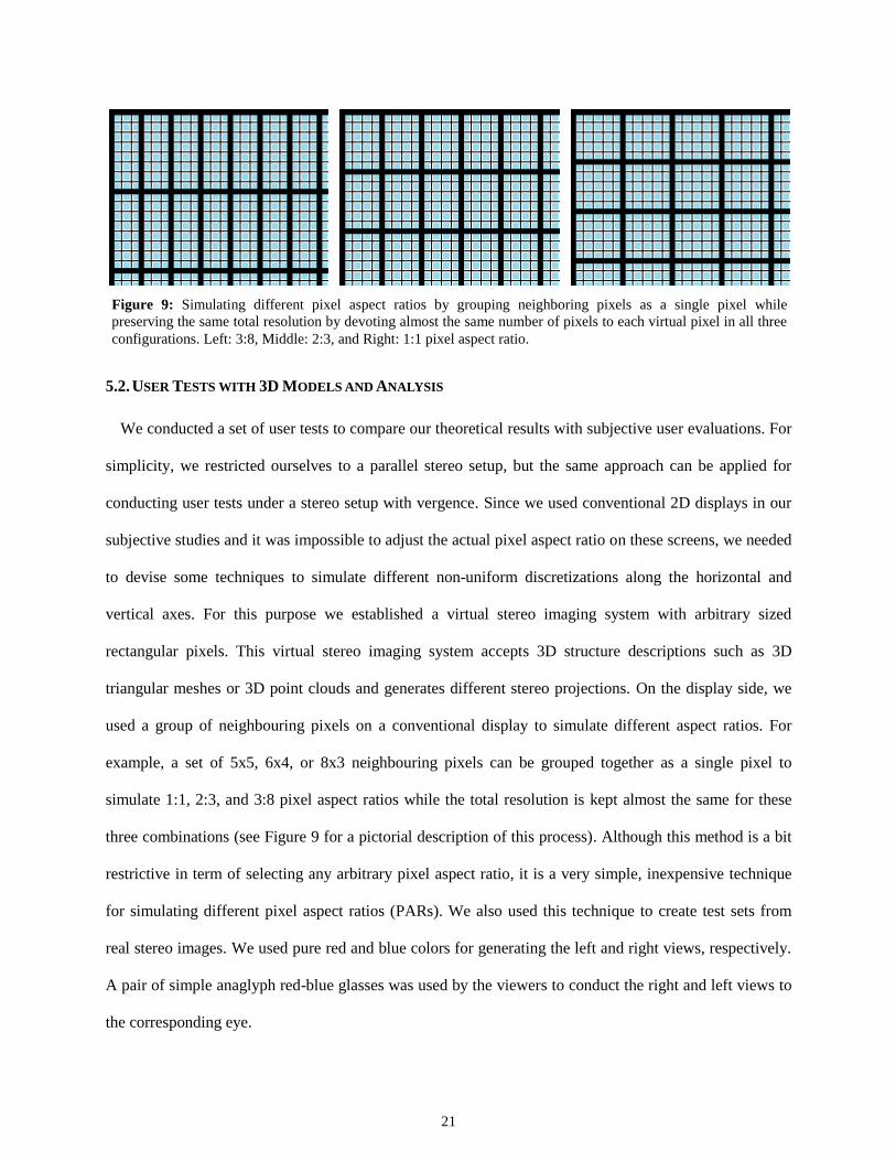
used a group of neighbouring pixels on a conventional display to simulate different aspect ratios. For
example, a set of 5x5, 6x4, or 8x3 neighbouring pixels can be grouped together as a single pixel to
simulate 1:1, 2:3, and 3:8 pixel aspect ratios while the total resolution is kept almost the same for these
three combinations (see Figure 9 for a pictorial description of this process). Although this method is a bit
restrictive in term of selecting any arbitrary pixel aspect ratio, it is a very simple, inexpensive technique
for simulating different pixel aspect ratios (PARs). We also used this technique to create test sets from
real stereo images. We used pure red and blue colors for generating the left and right views, respectively.
A pair of simple anaglyph red-blue glasses was used by the viewers to conduct the right and left views to
the corresponding eye.
Figure 9: Simulating different pixel aspect ratios by grouping neighboring pixels as a single pixel while
preserving the same total resolution by devoting almost the same number of pixels to each virtual pixel in all three
configurations. Left: 3:8, Middle: 2:3, and Right: 1:1 pixel aspect ratio.

22
Experiment 1 - User Tests with Synthetic Stereo Images - Figure 10 shows a set of three red-blue
images generated from a synthetic 3D model with three different pixel aspect ratios ─ 3:8, 2:3 and 1:1.
These images are generated using our virtual stereo imaging system. The advantage of using synthetic
scenes is that the properties of the scene can be defined according to the targeted evaluation criteria. Here,
the model is composed of a set of 3D points which collectively describe a sphere with a radius of 19 cm
and an ellipsoid with semi-minors of 50, 15, and 35 cm. The centers of the sphere and ellipsoid are
located at a distance of 40 and 80 centimetres respectively from the stereo camera. Two arbitrary rotations
are also applied to the ellipsoid. The colors (intensities) are randomly assigned to the 3D scene points but
geometric shape of the objects is preserved by assigning the same color to points located on the same
orbit. For this test set, the imaging system is configured using the values shown in Table 1. Considering
the depth range filled by these two objects, the theoretical optimal aspect ratio is given by the first row in
Table 2, i.e. 0.6315, which is almost equivalent to an aspect ratio of 2:3 – the ratio that is used to generate
the middle image in Figure 10.
We used the images shown in Figure 10 to conduct our first set of user tests. These images were
numbered from 1 to 3 from left to right. We followed the 3D visual experience model proposed in [16],
and asked the viewers to rank the images according to three criteria: sense of depth, picture quality and
overall sense. Sense of depth represents how objects are distinguishable and well-shaped across the depth
dimension. Picture quality refers to the quality of the perceived image which may be influenced by
several factors such as blockiness, brightness, noise and blurriness. Here, the picture quality is affected
Figure 10: Red-blue stereo pairs generated from a synthetic 3D scene with different aspect ratios. Left 3:8 (pixel
width: pixel height), middle 2:3, and right 1:1.
23
mainly by the non-similar discretization across the vertical and horizontal dimensions. Overall sense
measures a viewer’s overall satisfaction with each of these three 3D representations.
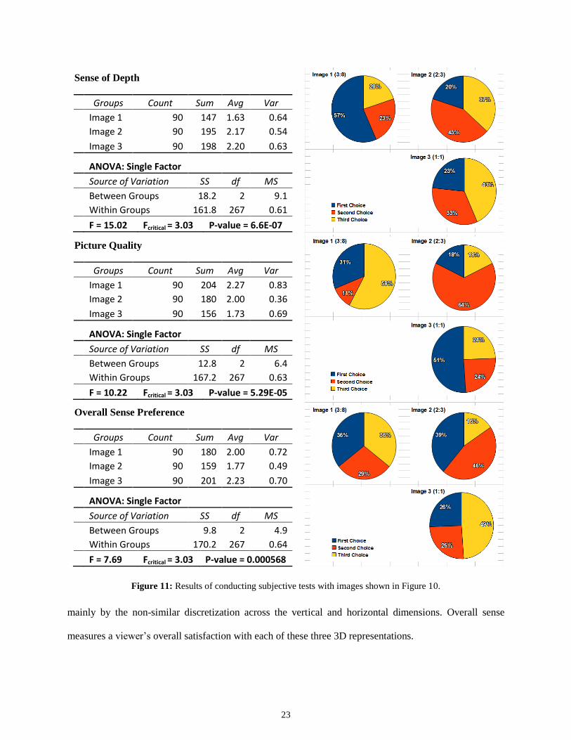
Figure 11: Results of conducting subjective tests with images shown in Figure 10.
Sense of Depth
Groups Count Sum Avg Var
Image 1 90 147 1.63 0.64 Image 2 90 195 2.17 0.54 Image 3 90 198 2.20 0.63
ANOVA: Single Factor
Source of Variation SS df MS
Between Groups 18.2 2 9.1 Within Groups 161.8 267 0.61
F = 15.02 Fcritical = 3.03 P-value = 6.6E-07
Picture Quality
Groups Count Sum Avg Var
Image 1 90 204 2.27 0.83 Image 2 90 180 2.00 0.36 Image 3 90 156 1.73 0.69
ANOVA: Single Factor
Source of Variation SS df MS
Between Groups 12.8 2 6.4 Within Groups 167.2 267 0.63
F = 10.22 Fcritical = 3.03 P-value = 5.29E-05
Overall Sense Preference
Groups Count Sum Avg Var
Image 1 90 180 2.00 0.72 Image 2 90 159 1.77 0.49 Image 3 90 201 2.23 0.70
ANOVA: Single Factor
Source of Variation SS df MS
Between Groups 9.8 2 4.9 Within Groups 170.2 267 0.64
F = 7.69 Fcritical = 3.03 P-value = 0.000568
24
Fifteen subjects (university graduate students) participated in our experiments. None of them were
aware of the judgments made by other participants and did not know the parameters used to create these
three images. Before ranking, we asked all participants to describe the reconstructed 3D scene to make
sure that all of them were able to clearly perceive the 3D scene composed of the ellipsoid and the sphere
in front it. Then we asked them to look at the 3D pictures as many times as they needed to decide on the
rankings. Since the entire screen was needed to display an image, the viewers were asked to switch
forward and backward to view all three images for comparison. A 14.1” display with 1280x800 resolution
is used for this experiment.
The pie charts in Figure 11 illustrate the result of this subjective study. The figure also presents some
statistics for each evaluation criterion including mean and variance in each group (image) and results of
analysis of variance (ANOVA test) for comparing means of groups. These results suggest a correlation
between the sense-of-depth and pixel aspect ratio. As depicted in the top-left graph, 57 percent of viewers
have the best sense of depth with Image 1 which has a pixel aspect ratio of 3:8, 20 percent have the best
sense of depth in Image 2 with pixel aspect ratio 2:3, and 23 percent selected Image 3 with a regular 1:1
pixel aspect ratio. In other words, a majority of the viewers preferred Image 1, which has the finest
horizontal resolution, as their first choice. As suggested by ANOVA test it is very unlikely (P-value =
6.6E-07) that the results obtained for Image 1, Image 2, and Image 3 to be belong to the same distribution.
In other words, it is very unlikely that users have selected images by chance. On the average, Image 1 is
selected as the first choice with significant difference and Image 2 as the second preference, even though
the difference between Image 2 and Image 3 is not statistically significant. This result, in general, is
consistent with our theoretical results that images with horizontally finer resolution provide better
sensation of depth. Some environmental and individual factors may explain why some people (the
minority) preferred Image 3. Since the human visual system varies from one person to another, we could
not fix a viewing distance for the best stereo effect. During the experiments, the viewers’ body positions
and movements could have affected the visual effect. Also, the capability of perceiving stereo effect
varies among the subjects. The small visual differences between the images might not be detectable to all
25
viewers. For small visual differences, it is worth mentioning that there were circumstances where the
viewers could not distinguish the sense of depth between two images. In these cases, we assigned equal
ranking to both images.
For ranking against picture quality (Figure 11 second row), viewers were asked to rank images
regardless of any perception of depth. Again, the results show meaningful but reverse relationship
between pixel aspect ratio and picture quality. More than 50 percent selected Image 3 for the best picture
quality. As discussed earlier in Section 3, this may be the result of image degradation that happens in the
vertical direction when the discretization becomes coarser in that direction, and as a result the Y
component estimation error might be increased. However, this trade-off of obtaining finer horizontal
discretization by sacrificing some quality in the Y component improves both the X and Z components, and
therefore the viewers have better overall sense in Image 1 and Image 2 which have non-uniform
discretization (Figure 11 third row). We observe in Figure 11 that in terms of overall sense, Image 2 with
aspect ratio 2:3 was the first or second choice for most of the viewers. This result illustrates certain
compromise in the viewers’ decisions towards the trade-off between sense of depth and picture quality. It
should be noted that the ANOVA test again rejects the null hypothesis of obtaining these results by
(d)
(b)
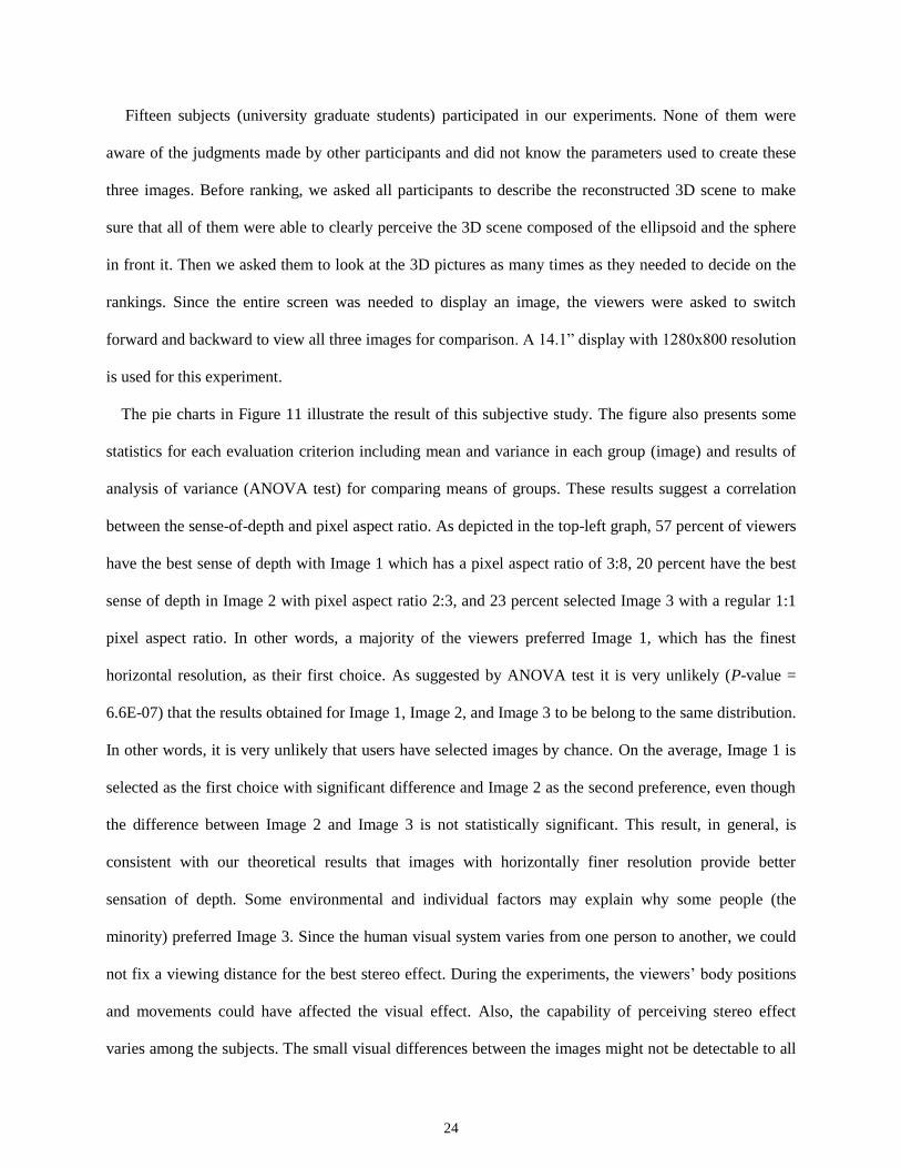
Figure 12: Samples generated from the Chinese Dragon 3D point cloud. (a) Original 3D object (red channel
projection), (b) 1:4, (c) 1:1, and (d) 4:1 pixel aspect ratios.
(a)
(c)
26
chance for both picture quality (P-value = 5.29E-05) and overall sense preference (P-value =0.000568)
criteria.
Figure 12 represents more clearly the image quality degradation in the vertical or horizontal direction
for a coarser discretization. These images are generated from Chinese Dragon 3D point cloud using our
virtual stereo imaging system with 1:4, 1:1, and 4:1 pixel aspect ratios, respectively, with the same total
resolution. For the 1:4 image (Figure 12-b) the discretization is more apparent along horizontal lines. For
example, observe the horizontal supplementary tail over the vertebral line of the dragon. On the other
hand, for the 4:1 image (Figure 12-c) the degradation is more apparent along vertical lines. Observe the
dragon’s vertical tail as an example. Both these images reveal lower image quality in some parts compare
to the uniform pixel discretization in the 1:1 image (Figure 12-d). In general, for complex scenes
composed of a set of edges, line, or textural features, depending on the feature directions, non-uniform
pixel discretization may degrade the picture quality in parts while quality may be improved in some other
areas. However, since a finer resolution on the horizontal direction also improves 3D estimation (sense of
depth), in overall, a better 3D picture is experienced when an appropriate aspect ratio is selected.
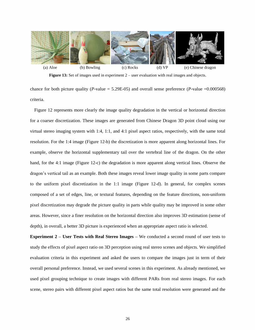
Experiment 2 – User Tests with Real Stereo Images – We conducted a second round of user tests to
study the effects of pixel aspect ratio on 3D perception using real stereo scenes and objects. We simplified
evaluation criteria in this experiment and asked the users to compare the images just in term of their
overall personal preference. Instead, we used several scenes in this experiment. As already mentioned, we
used pixel grouping technique to create images with different PARs from real stereo images. For each
scene, stereo pairs with different pixel aspect ratios but the same total resolution were generated and the
Figure 13: Set of images used in experiment 2 – user evaluation with real images and objects.
(a) Aloe (b) Bowling (c) Rocks (d) VP (e) Chinese dragon
27
users were asked to choose their preferred ones in a pair-wise manner. More precisely, assuming that I1,
I2, and I3 are the three stereo images generated for scene S with three different PARs 1:1 (5x5), 2:3 (6x4),
and 3:8 (8x3), we created three pairs I1I2 (or I2I1), I2I3 (or I3I2), and I1I3 (or I3I1) of these images (the order
of images are picked by random). Images (b), (c), (d), and (e) of Figure 13 are used for generating these
test cases. We put all these pairs together and shuffled them to form the test set. We enriched the test set
by randomly interleaving some other cases that were generated with some finer total resolutions to
examine how users will treat the images when the noise introduced by pixel grouping technique is less
apparent. These finer test cases were generated from images (a), (b), (c), and (d) of Figure 13. These test
cases were generated by grouping 4x4 and 5x3 pixels to examine 1:1 PAR versus 3:5 (~2:3) PAR, and by
grouping 3x3 and 4x2 pixels to compare 1:1 PAR versus 1:2 PAR.
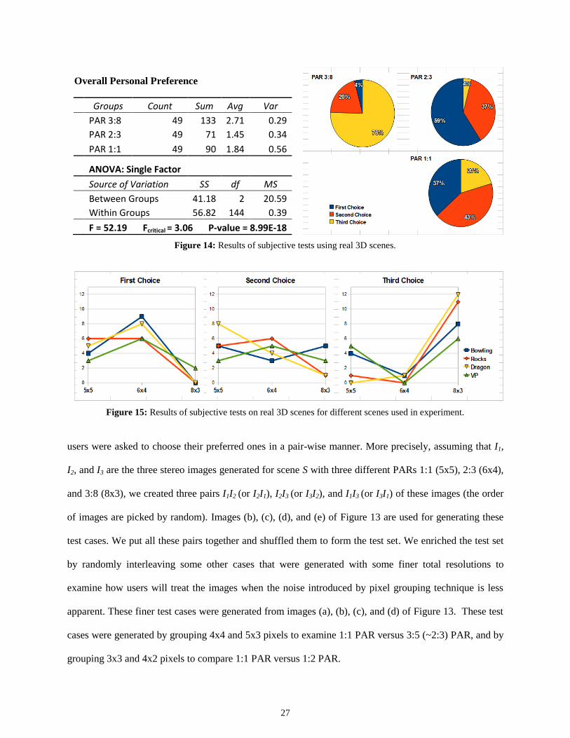
Overall Personal Preference
Groups Count Sum Avg Var
PAR 3:8 49 133 2.71 0.29 PAR 2:3 49 71 1.45 0.34 PAR 1:1 49 90 1.84 0.56
ANOVA: Single Factor
Source of Variation SS df MS
Between Groups 41.18 2 20.59 Within Groups 56.82 144 0.39
F = 52.19 Fcritical = 3.06 P-value = 8.99E-18
Figure 14: Results of subjective tests using real 3D scenes.
Figure 15: Results of subjective tests on real 3D scenes for different scenes used in experiment.

28
Thirteen subjects are participated in this experiment, majority of them university graduate students.
During the test, the users are asked to show their preference toward one of the stereo images in each pair.
Similar to Experiment 1 we did not enforce any time limit but all subjects spent almost the same amount
of time (between 25 to 30 minutes) to evaluate all cases. We also did not enforce a specific viewing
distance but we recommended the viewing distance of 70-80 cm considering that we were using a wider
display screen (19” display) in this experiment.
Figure 14 shows the user evaluation results for 5x5, 6x4, and 8x3 groupings with some associated
statistics. As can be seen from the pie charts, the results are greatly different for these three groups in
favour of the images with pixel aspect ratio 2:3 (6x4 pixel grouping). The outcome of the ANOVA test (F
= 52.19, P-value = 8.99E-18) also confirms the substantial difference between groups. PAR 2:3 not only
has been selected as the first choice by many viewers (59%) but also rarely has been the third choice of
viewers (4%). In other words, in 96% of cases images with PAR 2:3 are selected either as first or second
preferred image.
In contrast to the results of Experiment 1 (synthetic scene), here images with PAR 1:1 (i.e. images with
uniform pixel distribution) have mainly owned the second place (43%) and images with PAR 3:8 have
often been selected as the least favourite ones (76%). This can be explained by the way that pixel
grouping technique treats image features. In fact, since the real images we have used in this experiment
possess more textural or structural features, comparing to the simple synthetic scene of Experiment 1 that
is composed of poorly featured geometrical objects, they are more prone to the noise introduced by
sharper simulated PARs.
Figure 15 shows a more detailed representation of the results presented in Figure 14 pie charts. The line
charts of this figure show how different scenes are treated by viewers. In general, the drawings show a
consistent behaviour toward all four different scenes that are used in this experiment. However, the results
seem to be a little affected by the scene structures. For example, the users have had tendency to select the
Rocks scene with more horizontally oriented edges and textural features, as their first choice than the VP
29
scene with more vertically aligned structures. However, the differences are not that much that contradicts
each other and the expected theoretical results.
We separately analysed the results of test cases with finer total resolution. For 3x3 verses 4x2 test
cases, 54% of viewers were in favour of images with uniform pixel distribution (3x3, 1:1 PAR). We did
not find statistically significant difference between these two groups. However, at least we can say that
the images with 1:2 PAR (4x2) with less apparent pixel grouping noise have received much more
attention when they are compared with the images of corresponding uniform pixel distribution than
images with 3:8 PAR (8x3). For 4x4 versus 5x3 cases we found that 63% of viewers were in favour of
images with non-uniform pixel distribution (5x3, 3:5 PAR) with statistically significant difference
between two groups (paired T-Test P-value = 0.01). These results are consistent with the results obtained
for images with the same PARs but coarser total resolution (see pie charts in Figure 14).
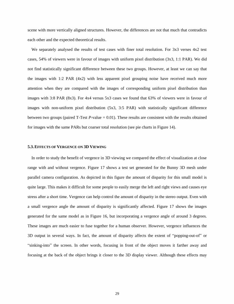
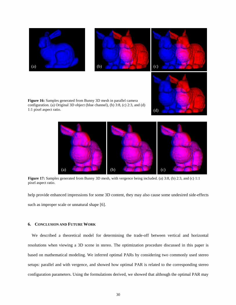
5.3. EFFECTS OF VERGENCE ON 3D VIEWING
In order to study the benefit of vergence in 3D viewing we compared the effect of visualization at close
range with and without vergence. Figure 17 shows a test set generated for the Bunny 3D mesh under
parallel camera configuration. As depicted in this figure the amount of disparity for this small model is
quite large. This makes it difficult for some people to easily merge the left and right views and causes eye
stress after a short time. Vergence can help control the amount of disparity in the stereo output. Even with
a small vergence angle the amount of disparity is significantly affected. Figure 17 shows the images
generated for the same model as in Figure 16, but incorporating a vergence angle of around 3 degrees.
These images are much easier to fuse together for a human observer. However, vergence influences the
3D output in several ways. In fact, the amount of disparity affects the extent of “popping-out-of” or
“sinking-into” the screen. In other words, focusing in front of the object moves it farther away and
focusing at the back of the object brings it closer to the 3D display viewer. Although these effects may
30
help provide enhanced impressions for some 3D content, they may also cause some undesired side-effects
such as improper scale or unnatural shape [6].
6. CONCLUSION AND FUTURE WORK
We described a theoretical model for determining the trade-off between vertical and horizontal
resolutions when viewing a 3D scene in stereo. The optimization procedure discussed in this paper is
based on mathematical modeling. We inferred optimal PARs by considering two commonly used stereo
setups: parallel and with vergence, and showed how optimal PAR is related to the corresponding stereo
configuration parameters. Using the formulations derived, we showed that although the optimal PAR may
(a) (b) (c)
(d)
Figure 16: Samples generated from Bunny 3D mesh in parallel camera
configuration. (a) Original 3D object (blue channel), (b) 3:8, (c) 2:3, and (d)
1:1 pixel aspect ratio.
(a) (b) (c)
Figure 17: Samples generated from Bunny 3D mesh, with vergence being included. (a) 3:8, (b) 2:3, and (c) 1:1
pixel aspect ratio.
31
considerably vary with different parameter values, in general, for a given total resolution a more dense
distribution of pixels along the horizontal direction often improves the sense of depth and overall output
quality of the 3D display. Applying practical parameter values into inferred equations, we theoretically
suggested that a pixel aspect ratio of 2:3 ([pixel width]:[pixel height]) will lead to a better stereo-based
3D viewing experience. We validated the theoretical results through conducting subjective user
experiments on both synthetic and real stereo content with different simulated pixel aspect ratios. Our
experiments showed that from a subjective point of view the suggested optimal PAR indeed improves the
3D output.
Our method of simulating different PARs using pixel grouping introduces noticeable blockiness into
images. In this regard, it will be interesting to incorporate the concept of Just Noticeable Difference
(JND) for 3D perception [22] to see how the results may change. We expect that the whole effect of
applying optimal PAR on a high-resolution display lead to a noticeable improvement on the overall 3D
output quality, even though, the user may not be able to separately distinguish the pixels of such high-
resolution displays (similar to 2D displays that overall quality improves by increasing the resolution even
if the pixels are not distinguishable by viewers). It should also be clarified that the optimal PAR greatly
improves the resolution across the depth dimension. This is very important for many interactive stereo-
based 3D applications that usually suffer from low pointing accuracy across the depth. Optimal PAR
facilitates more accurate 3D pointing and hence more accurate 3D interaction and manipulation [27].
It will be also interesting to incorporate other factors such as different viewing conditions, human
perceptual factors [17][18][19][20], motion factors [21], and error measures produced by cross-talk,
correlation, and epipolar constraints [23][24], in order to derive more advanced models. Such models can
also take into account the relative importance of vertical vs. horizontal disparities for the human visual
system, and incorporate an image quality metric to reflect the picture quality changes caused by non-
uniform discretization. Moreover, our brief discussion on various aspects of introducing vergence into the
system can also be extended especially for large vergence angles and for scenes composed of multiple
objects with cameras focused on one of these objects.

32
The approach developed in this study could be extended to understand the cause of the anisotropy
[25][26] present between horizontal vs. vertical depth perception through stereo (or motion induced
stereo) in humans. Our analysis shows that considering practical 3D viewing distances, uniform
distribution of pixels on a sensor (display) produces better reconstruction results for the horizontal axis,
when the stereo baseline is along the horizontal axis. However, the analysis needs to be extended taking
into account the spatially varying distribution of cones in the human eye and possibly issues like “depth
consistency” in human perception. Finally, the analysis in this paper could be made more geometric by
considering “volumes of uncertainty” extending the approach discussed in [10].
Acknowledgments
The authors thank iCORE, Alberta and NSERC, Canada, for their research support. The authors also
thank the Stanford Computer Graphics Laboratory for providing the Bunny and the Chinese Dragon 3D
models (the Chinese Dragon is originally provided by XYZ RGB Inc.), and the Middlebury College for
providing some of the real 3D scenes that are used in user evaluations.
References
[1] D. F. McAllister, “Stereo computer graphics and other true 3D technologies”, Princeton University Press, 1993.
[2] K. Satoh and Y. Ohta, “Passive depth acquisition for 3D image displays”, IEICE transactions on Information
and System, September 1994.
[3] O. Schreer, P. Kauff and T. Sikora (Eds.), “3D Video Communication”, Wiley, 2005.
[4] W. Matusik, and H. Pfister, “3D TV: a scalable system for real-time acquisition, transmission, and
autostereoscopic display of dynamic scenes”, ACM Transactions on Graphics, 2004, volume23, pp 814-824.
[5] S. Baker, R. Szeliski and P. Anandan, “A Layered Approach to Stereo Reconstruction”, IEEE CVPR, 1998.
[6] B. Javidi, F. Okano, “Three-dimensional Television, Video, and Display Technologies”, Chapter 1, Springer,
2002.

33
[7] T. Mitsuhashi, “A study of the relationship between scanning specifications and picture quality,” NHK, NHK
Laboratories Note, no. 256, Oct. 1980.
[8] I. Cheng and A. Basu, “Optimal aspect ratio for 3D TV,” IEEE 3D TV Conference, 4 pages, KOS, Greece,
May 2007.
[9] A. Basu, “Optimal discretization for stereo reconstruction”, Pattern Recognition Letters, vol. 13, no. 11, pp
813-820, 1992.
[10] H. Sahabi and A. Basu, “Analysis of error in depth perception with vergence and spatially varying sensing”,
Computer Vision and Image Understanding, vol. 63, no. 3, May, pp. 447-461, 1996.
[11] N. Holliman, “3D display systems”, Department of Computer Science, University of Durham, Science
Laboratories, South Road, Durham, DH1 3LE; Feb 2, 2005; http://www.dur.ac.uk/n.s.holliman/
Presentations/3dv3-0.pdf.
[12] I. Cheng, K. Daniilidis, and A Basu, “Optimal Aspect Ratio under Vergence for 3D TV”, 3DTV Conference:
The True Vision - Capture, Transmission and Display of 3D Video, 2008, pp.209-212, 28-30 May 2008.
[13] A. Basu, and H. Sahabi, “Optimal Non-uniform discretization for Stereo Reconstruction”, Pattern Recognition,
1996, Proceedings of the 13th International Conference on, vol.1, pp.755-759 vol.1, 25-29 Aug 1996.
[14] M. Z. Brown, D. Burschka, and G. D. Hager, “Advances in Computational Stereo”, IEEE Transactions on
Pattern Analysis and Machine Intelligence, vol. 25, no. 8, August 2003.
[15] D. Scharstein, and R. Szeliski, “A Taxonomy and Evaluation of Dense Two-Frame Stereo Correspondence
Algorithms”, International Journal of Computer Vision”, vol. 47, pp. 7-42, 2002.
[16] P. J. H. Seuntins, “Visual experience of 3D TV”, Eindhoven: Technische Universiteit Eindhoven, 2006,
Proefschrift. http://alexandria.tue.nl/extra2/200610884.pdf.
[17] B.T. Backus, D.J. Fleet, A.J. Parker and D.J. Heeger, “Human Cortical Activity Correlates With Stereoscopic
Depth Perception,” The Journal of Neurophysiology, 2054-2068, October 2001.
[18] I. Cheng and A. Basu, “Perceptually Optimized 3D Transmission over Wireless Networks”, IEEE Transactions
on Multimedia, 386-396, 2007.
[19] L.-F. Cheong, “Depth perception under motion and stereo with implications for 3D TV”, 3D TV Conference,
Greece, 4 pages, May 2007.
34
[20] Y. Pan, I. Cheng and A. Basu, “Quality Metric for Approximating Subjective Evaluation of 3D Objects”, IEEE
Trans. on Multimedia, 269-279, April 2005.
[21] L.-F. Cheong, C. Fermüller and Y. Aloimonos, “Effects of errors in the viewing geometry on shape
estimation,” Computer Vision and Image Understanding, 356-372, Sep. 1998.
[22] I. Cheng and P. Boulanger, “A 3D Perceptual Metric using Just-Noticeable-Difference”, EUROGRAPHICS,
2005, Dublin, Ireland.
[23] T. Brodsky, C. Fermüller and Y. Aloimonos, “Structure from motion: Beyond the epipolar constraint,” Int.
Journal of Computer Vision, vol. 37, no. 3, 231-258, 2000.
[24] N. Ayache, “Artificial Vision for Mobile Robots: Stereo Vision and Multisensory Perception,” MIT Press,
1991.
[25] B.J. Rogers and M.E. Graham, “Anisotropies in the perception of three-dimensional surfaces,” Science, 221,
1409-1411, 1983.
[26] V. Cornilleau-Pérès and J. Droulez, “Visual perception of surface curvature: psychophysics of curvature
detection induced by motion parallax,” Perception and Psychophysics, 46: 351-364. 1989.
[27] Hossein Azari, Irene Cheng, and Anup Basu, “Stereo 3D Mouse Cursor: A Method for Interaction with 3D
Objects in a Stereoscopic Virtual 3D Space,” International Journal of Digital Multimedia Broadcasting, vol.
2010, Article ID 419493, 11 pages, 2010.

35
Appendix A
Derivation for Result 3:
00
max max max 0
0min max0
max 0
max max
min max
max
( )
22 ( )
2
( )
2 ( )
2 22 2 4 20
2
max 0
2 0
max 0
( ) 2
( )4 4
( )
4
( )
Z ZXX
Z y Z Z
xp x x
Z ZXZ yX
Z Z
Z y
xx x x
Z y
xx
y
fbF e y e R dXdydZ
Z
yZ Z f bX Re fb R e y dydZ
Z Z Z Z
yXZ Rfbe dydZ
Z Z Z
max max max max
min min max
max max max max
min max min max
max 0
224 2 20
0
max 0 max 0
4
( )
44
( ) ( )
Z y Z y
x
Z Z y
Z y Z y
x
Z y Z y
XRfby dydZ
Z Z
XR ZXRe Zy dydZ y dydZ I
Z Z Z Z
where I0 is independent of ex, and thus has no influence on the minimization of Fp(ex).
2 01 min max 2 min max
max 0 max 0
224 0
3 min max 4 min max 0
max 0 max 0
4 4( ) [ , ] [ , ]
( ) ( )
44[ , ] [ , ]
( ) ( )
x xp x x
x
XZ Rfb XRfbF e e I Z Z I Z Z
Z Z Z Z
XR ZXRe I Z Z I Z Z I
Z Z Z Z
where I1 to I4 are integrals defined in Result 3.
Considering the derivative of Fp(ex) in terms of ex and equating it to zero, we have:
0
],[4
],[4
4
],[4
],[4
2
maxmin4
0max
0
2
maxmin3
0max
23
maxmin2
0max
maxmin1
0max
0
ZZIZZ
ZXRZZI
ZZ
XRe
ZZIZZ
XRfbZZI
ZZ
RfbXZeeF
x
xxxxp
.
Since we cannot take ex = 0 as the optimal point, we should have:
0],[],[Re2],[],[ maxmin40maxmin3
2
maxmin2maxmin10 ZZIZZZIZZIZZIZfb xx
Solving this equation in terms of ex, and again considering that we cannot take negative values for ex as
the optimal point, we obtain the following equation (or Equation 29) as the possible optimal point:
xOptx
x eZZIZZZI
ZZIZZIZ
R
fbe
2
1
maxmin40maxmin3
maxmin2maxmin10
],[],[
],[],[
2.
36
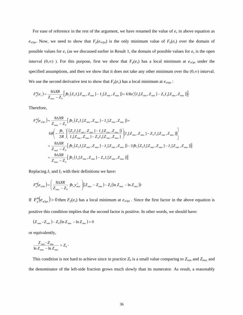
For ease of reference in the rest of the argument, we have renamed the value of ex in above equation as
exOpt. Now, we need to show that Fp(exOpt) is the only minimum value of Fp(ex) over the domain of
possible values for ex (as we discussed earlier in Result 1, the domain of possible values for ex is the open
interval (0,∞) ). For this purpose, first we show that Fp(ex) has a local minimum at exOpt under the
specified assumptions, and then we show that it does not take any other minimum over the (0,∞) interval.
We use the second derivative test to show that Fp(ex) has a local minimum at exOpt :
],[],[Re6],[],[8
maxmin40maxmin3
2
maxmin2maxmin10
0max
ZZIZZZIZZIZZIZfbZZ
XReF xxxp
.
Therefore,
],[],[8
],[],[3],[],[8
],[],[],[],[
],[],[
26
],[],[8
maxmin10maxmin2
0max
maxmin2maxmin10maxmin2maxmin10
0max
maxmin40maxmin3
maxmin40maxmin3
maxmin2maxmin10
maxmin2maxmin10
0max
ZZIZZZIfbZZ
XR
ZZIZZIZfbZZIZZIZfbZZ
XR
ZZIZZZIZZIZZZI
ZZIZZIZ
R
fbR
ZZIZZIZfbZZ
XReF
x
xx
x
xxOptp
Replacing I1 and I2 with their definitions we have:
minmax0minmax
2
max
0max
lnln8
ZZZZZyfbZZ
XReF xxOptp
.
If 0xOptp eF then Fp(ex) has a local minimum at exOpt . Since the first factor in the above equation is
positive this condition implies that the second factor is positive. In other words, we should have:
0lnln minmax0minmax ZZZZZ
or equivalently,
0
minmax
minmax
lnlnZ
ZZ
ZZ
.
This condition is not hard to achieve since in practice Z0 is a small value comparing to Zmin and Zmax and
the denominator of the left-side fraction grows much slowly than its numerator. As result, a reasonably

37
large viewing volume in the direction of the Z axis easily satisfies this condition and so Fp(exOpt) will be a
local minimum under this assumption.
Following the same procedure as above for the other two extrema (i.e., ex = 0 and ex = -exOpt), it is not
difficult to show that under the same assumption Fp(0) and Fp(-exOpt) are local maximum and local
minimum, respectively. Therefore, considering that Fp(-exOpt), Fp(0), and Fp(exOpt) are the only local
extrema of function Fp(ex), Fp(exOpt) should be the only minimum (or equivalently a global minimum) over
open interval (0,∞).
Derivation for Result 4:
2
2( ) 2xv x x
Z y X
fbF e RKe y dXdydZ
Z
Case I) Zint ≤ Zmin
Considering the equations in AR5 (page 16), the integral in Equation 34 should be calculated according
to the following range of values:
intmax max
int
min maxint
int
1 2( )
2 2
1( )
2
( ) 2x x
x x
ZX b bZ y Z x
v x xZZ y X b bZ
fbF e RKe y dXdydZ
Z
Thus,
max max
min max
2 22 2 2 4 2
int 2
int
2 2 int1 min max 2 min max
int
2 24 2 2int
3 min max
int
( ) ( ) 4 4
4( )4 [ , ] [ , ]
4( )[ , ] 4
Z y
xv x x x x x x
Z y
x xx x
xx x
yf bZF e X b b RKe fb R K e y dydZ
Z Z Z
X b RKfbe RKfb I Z Z I Z Z
Z
X b R Ke I Z Z R K b I
Z
4 min max 0[ , ]Z Z I
where again I0 is independent of ex and has no effect on optimization of Fv(ex), and I1 to I4 are defined as
in Result 3.
38
0
],[4],[)(4
4
],[)(4
],[42
maxmin4
22
maxmin3
int
22
int3
maxmin2
int
int
maxmin1
2
ZZIbKRZZIZ
KRbXe
ZZIZ
RKfbbXZZIRKfbeeF
x
x
x
xx
xxxv
or
2 2int int1 min max 2 min max 3 min max 4 min max
int int
( ) 4( )[ , ] [ , ] 2 [ , ] [ , ] 0x x x
x x x
X b fb X b RKfb I Z Z I Z Z e I Z Z RKb I Z Z
Z Z
.
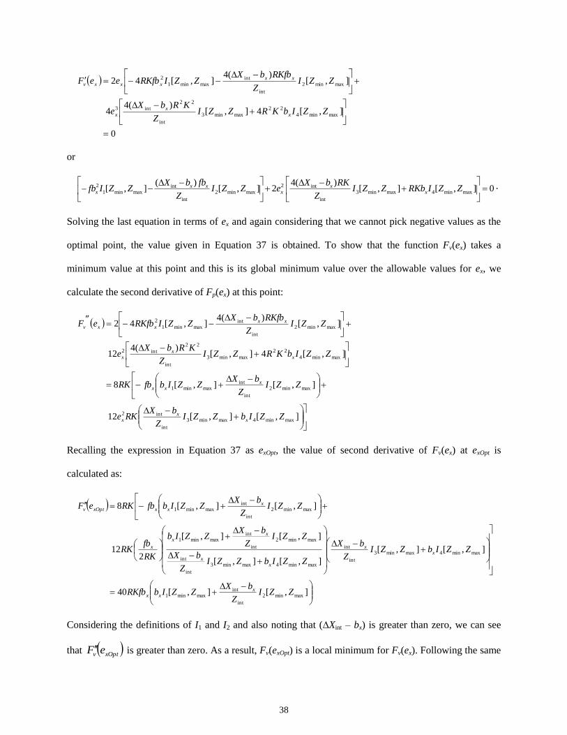
Solving the last equation in terms of ex and again considering that we cannot pick negative values as the
optimal point, the value given in Equation 37 is obtained. To show that the function Fv(ex) takes a
minimum value at this point and this is its global minimum value over the allowable values for ex, we
calculate the second derivative of Fp(ex) at this point:
],[],[12
],[],[8
],[4],[)(4
12
],[)(4
],[42
maxmin4maxmin3
int
int2
maxmin2
int
intmaxmin1
maxmin4
22
maxmin3
int
22
int2
maxmin2
int
intmaxmin1
2
ZZIbZZIZ
bXRKe
ZZIZ
bXZZIbfbRK
ZZIbKRZZIZ
KRbXe
ZZIZ
RKfbbXZZIRKfbeF
xx
x
xxx
xx
x
xxxxv
Recalling the expression in Equation 37 as exOpt, the value of second derivative of Fv(ex) at exOpt is
calculated as:
],[],[40
],[],[
],[],[
],[],[
212
],[],[8
maxmin2
int
intmaxmin1
maxmin4maxmin3
int
int
maxmin4maxmin3
int
int
maxmin2
int
intmaxmin1
maxmin2
int
intmaxmin1
ZZIZ
bXZZIbRKfb
ZZIbZZIZ
bX
ZZIbZZIZ
bX
ZZIZ
bXZZIb
RK
fbRK
ZZIZ
bXZZIbfbRKeF
xxx
xx
xx
xx
x
xxxxOptv
Considering the definitions of I1 and I2 and also noting that (∆Xint – bx) is greater than zero, we can see
that xOptv eF is greater than zero. As a result, Fv(exOpt) is a local minimum for Fv(ex). Following the same

39
procedure for the other two extrema, it is not difficult to show that Fv(0) and Fv(-exOpt) are local maximum
and local maximum, respectively. Since Fv(-exOpt), Fv(0), and Fv(exOpt) are the only extrema of Fv(ex), we
can say that Fv(exOpt) is a global minimum over the interval (0,∞).
Case II) Zmax ≤ Zint
In this case following integral should be calculated:
0int
max maxint 0
0min maxint
int 0
max max
min max
1 2
2 2
1
2
2 22 2 2 4 20
int 2
int 0
( ) 2
4 4
Z ZXZ y Z Z x
v x xZ ZZ y XZ Z
Z yx
x x xZ y
fbF e RKe y dXdydZ
Z
yZ Z f bX RKe fb R K e y dydZ
Z Z Z Z
.
Similar to Case I, calculating the derivative of Fv(ex) and equating it to zero gives the result. To show that
the expression obtained, i.e. Equation 38, minimizes Fv over the domain of allowable values for ex, the
same argument as in Result 3 should be applied. The assumption of choosing a large enough volume
along with the Z dimension is also needed to be considered for this case. Because of many similarities
with the derivation for Result 3 the details are skipped here.
Case III) Zmin < Zint < Zmax
In this case the integral in Equation 34 should be divided into two parts as follow. The other steps are
similar to the Cases I and II and are skipped here.
max
int
max
max
intint2
1
intint2
1
int
min
max
max
0int
0int2
1
0int
0int2
1
)(
)(
2
2
2
2 22Z
Z
y
y
bbX
bbXx
xZ
Z
y
y
X
Xx
x
xv
xZ
Zx
xZ
Zx
ZZ
ZZ
ZZ
ZZdXdydZyRKe
Z
fbdXdydZyRKe
Z
fbeF .