Embed Size (px)
Citation preview

Optimal Base Station Selection for Anycast Routingin Wireless Sensor Networks 指導教授 : 黃培壝 & 黃鈴玲
學生 : 李京釜

Author & Source
Source : IEEE TRANSACTIONS ON VEHICULAR TECHNOLOGY, VOL. 55, NO. 3, MAY 2006
Author : Y. Thomas Hou, Senior Member, IEEE, Yi Shi, Student Member, IEEE, and Hanif D. Sherali

Outline
1. Introduction
2. REFERENCE NETWORK MODEL AND
PROBLEM DESCRIPTION
3. PROBLEM FORMULATION AND AN UPPER BOUND FOR OPTIMAL SOLUTION

Outline
4. ABS: A HEURISTIC ALGORITHM
5.Performance Evaluation & Simulation Results
6. CONCLUSION
Introduction
Wireless sensor networks consist of battery-powered nodes including multimedia (e.g., video and audio) and scalar data (e.g., temperature, pressure).
There has been active research on exploring optimal flow routing strategies to maximize the lifetime of the network .

Introduction
A sensor network having only a single sink node , all the data traffic generated by the sensor nodes will be delivered to this sink node.
Having multiple sink nodes, the data traffic generated by any sensor node may be split and sent to multiple different BSs.

Introduction
BS is chosen as the destination sink node have a impact on the overall network lifetime performance.
It appears to understand how to perform anycast in energy-constrained sensor networks.
Introduction
We investigate the optimal BS selection problem for anycast with the aim of maximizing network lifetime.

Reference network model
1. Microsensor nodes (MSNs)MSN is to collect data and send it directly to the local AFN.
2. AFNs. data aggregation for information flows coming from the local cluster of MSNs. Forwarding the aggregated information to the next hop AFN (toward a BS).

Reference network model
3. BSsBSs are the sink nodes for all the data collected in the network.


Problem Description

Problem Description

Problem Description
Pt(i, k) = cik ・ fik …(1)
Pt(i, k) is the power dissipated at AFN i when it is transmitting to node k, fik is the bit rate tra
nsmitted from AFN i to node k, and cik is the power consumption cost of radio link (i, k).

Problem Description
cik = α + β ・ … (2) Where α and β are constants, is the distance betwee
n node i and node k, and m is the path loss index.
Pr(i) = …(3) Where (bts/s) is the aggregate rate of the recei
ved data streams by AFN i.
kik i
f
kik i
f
mikd
mikd

Problem description
The anycast problem is an optimal mapping between an AFN and a BS such that the network lifetime can be maximized.
The first component involves the mapping between each AFN and a particular BS.

Problem description
The second component is to perform flow routing for a given mapping such that the network lifetime can be maximized.
Video is necessary to forward all bit streams generated by an AFN to the same BS (instead of to different BSs).

Problem description
The bit stream from AFN can be split into subflows and sent to the same BS through different paths.
Advantage : more flexible and energy “wise”.
Disadvantage : delay jitter and thus require playout buffer at the BS.

Problem Formulation

Problem Formulation

ABS: A HEURISTIC ALGORITHM 1) Solve the LP-Relax problem.
2) Fix some AFNs’ BS via the solution to the LP-Relax problem as follows,a) If there exists some AFN i that sends at least θ percentage
of its data to one BS, i.e., λAiBl (= (μAiBl )/T ) ≥ θ, select this BS as its destination.

ABS: A HEURISTIC ALGORITHM b) Else, i.e., there is no AFN that sends at lea
st θ percentage of its data to one BS, denote
μAiBl as the largest among all μ values and select Bl as AFN i’s destination.

ABS: A HEURISTIC ALGORITHM 3) If all AFNs’ destinations are fixed, stop; oth
erwise, reformulate the LP-Relax problem. In this LP-Relax, if AFN i’s destination is fixed a
s Bl, then μAiBl = T (i.e.,λAiBl = 1) and all other μ variables for AFN i are zero.
4) Go to Step 1.

ABS: A HEURISTIC ALGORITHM In Step 2(b) the largest traffic volume sent by
AFN i to a BS is comparable to the second largest traffic volume sent by AFN i to a different BS.
The distance factor should be taken into consideration since doing so would help reduce energy consumption.

Simulation Settings
N = 10, 20, and 30 AFNs along withM = 4, 5, and 6 BSs.
We run ten experiments (each under a randomly generated network topology for the AFNs), thus obtaining 90 sets of data.
Simulation Settings
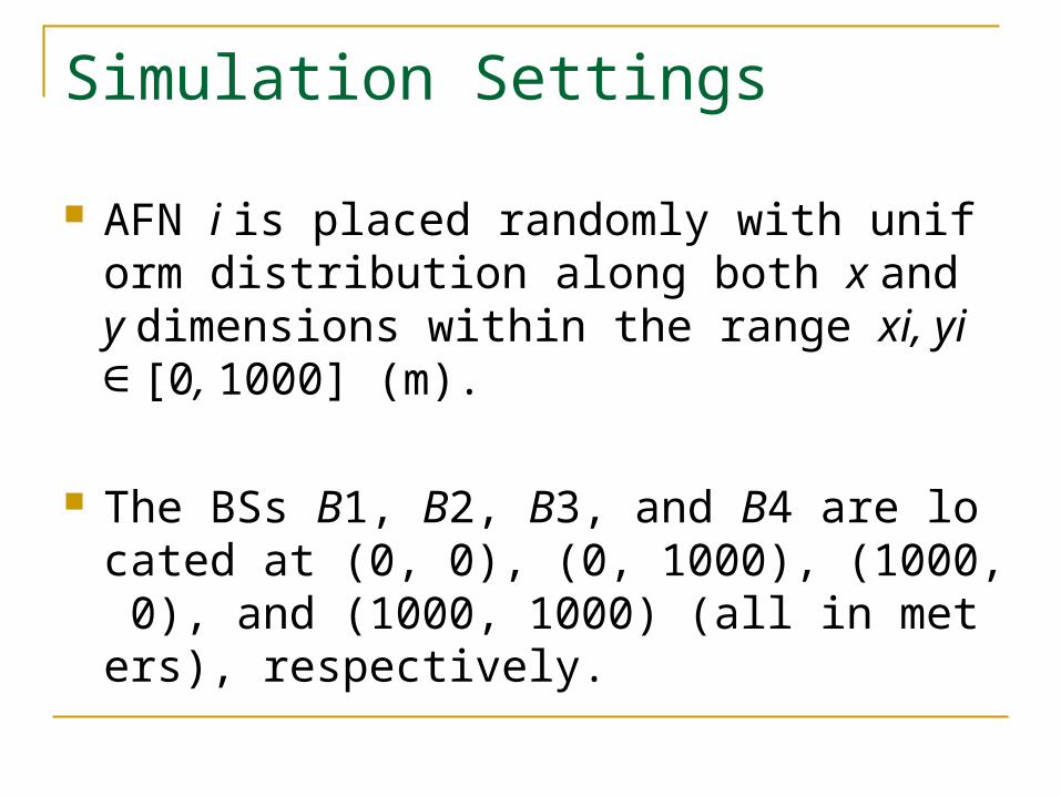
AFN i is placed randomly with uniform distribution along both x and y dimensions within the range xi, yi ∈ [0, 1000] (m).
The BSs B1, B2, B3, and B4 are located at (0, 0), (0, 1000), (1000, 0), and (1000, 1000) (all in meters), respectively.

Simulation Settings
When there are five BSs present, B is located at (500, 500); when there are six BSs present, B5 and B6 are located at (0, 500) and (1000, 500), respectively.
The initial energy at AFN i is also randomly generated following a uniform distribution with ei ∈ [250, 500] (kJ).

Simulation Settings
The data rate generated by AFN i, gi, is also uniformly distributed within [2, 10] (kb/s).
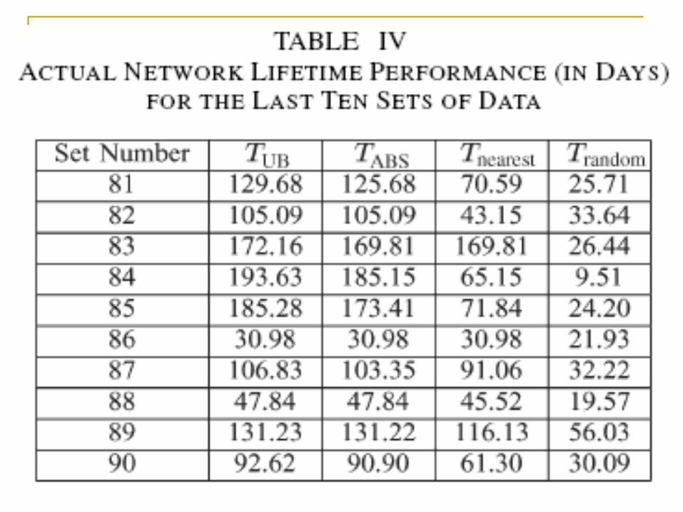
TABS as the network lifetime obtained via our ABS algorithm.

Performance evalution
Tnearest : AFN i simply chooses the nearest BS as its anycast BS.
Trandom : AFN i chooses a random BS as its anycast BS.

Performance evalution
Network lifetimes as
TUB= 52.31 days
LABS = TABS/TUB,
Lnearest = Tnearest/TUB,
Lrandom =Trandom/TUB.


Performance Evalution
It is easy to verify that for each AFN, the flow balance holds at any time during [0, 49.93] days and that the energy constraint is satisfied over 49.93 days.

Simulation Results
TABS = 49.93 days by solving the LP-Routing problem.
LABS = 49.93/52.31 = 95.45%.
Tnearest = 23.34 days for the nearest BS selection approach

Simulation Results
Trandom = 12.08 days for the random BS selection approach.
Lnearest = 44.61% and Lrandom = 23.09%.


Performance Evaluation

Conclusion
We proposed a heuristic algorithm called ABS that has polynomial time complexity and to maximize network lifetime.
Simulation results show that this algorithm has near-optimal performance and is superior than some other approaches.