Embed Size (px)
Citation preview

Optimal Cluster Number Selection in Ad-hoc Wireless Sensor Networks
1,3 1,2 4 5 1Tung-Jung Chan, Ching-Mu Chen, Yung-Fa Huang, Jen-Yung Lin and Tair-Rong Chen 1Department of Electrical Engineering,
National Changhua University of Education,
Bao-Shan Campus: No.2, Shi-Da Road, Changhua City 500,
Taiwan, R.O.C.
[email protected] 2 Department of Computer Science and Information Engineering,
3 Department of Electrical Engineering,
Chung Chou Institute of Technology,
No. 6, Lane 2, Sec. 3, Shanjiao Rd., Yuanlin Township, Changhua County 510,
Taiwan, R.O.C.
{kchen, jung}@dragon.ccut.edu.tw 4 Graduate Institute of Networking and Communication Engineering,
Chaoyang University of Technology,
168 Jifong E. Rd., Wufong Township Taichung County, 41349,
Taiwan, R.O.C.
[email protected] 5 Department of Computer Science and Information Engineering,
Dayeh University,
No. 112, Shanjiao Rd., Dacun, Changhua, Taiwan, 51591,
Taiwan, R.O.C.
Abstract: - In clustering-based wireless sensor networks (WSNs), a certain sensing area is divided into many
sub-areas. Cluster formation and cluster head selection are well done in the setup phase. With the pre-
determined probability and random, every round in the WSNs has the different cluster numbers and cluster
heads. However, the well known technique in cluster-based WSN is especially the low energy adaptive cluster
hierarchy (LEACH) and its energy performance is improved due to the scheme of clustering, probability, and
random. The clustering-based WSN has sensor nodes organized themselves with the pre-determined variable p
to form clusters. With the pre-determined p variable and probability, every round has different cluster numbers
which are not the optimal solution. Therefore, in order to evenly consume nodes’ energy, this paper proposes a
fixed optimal cluster (FOC) numbers that is to analyze the entire network first to have the optimal cluster
numbers and then apply it to form the optimal cluster numbers. Moreover, there are two different types of the
optimal cluster numbers depending on the location of the base station. One is that the base station is setup at the
center of the sensing area. The other is that the base station is setup at the far way of the sensing area. Finally,
by the optimization analysis of cluster numbers applied to the ad-hoc WSN before sensor nodes are randomly
deployed, the simulation results show the entire network lifetime can be extended very well.
Key-Words: - Ad-hoc Wireless sensor networks, Analysis, Optimal Cluster numbers, Energy efficiency,
Clustering-based, Pre-determined variable, Random, Base station location.
1 Introduction Due to the technology improved quickly [1], sensor
nodes are becoming smaller and smaller. With this
tiny sensor node, it contains the power supply unit,
processing unit, receiver unit, transceiver with
amplifier unit and antenna unit as shown in Fig. 1.
In recent years, not only the sensor node become
smaller, but also it comes with the characteristics of
chips smaller and faster, less power needed and
transmission distance longer because of the advance
technology. By these characteristics of sensor nodes
WSEAS TRANSACTIONS on COMMUNICATIONS
Tung-Jung Chan, Ching-Mu Chen, Yung-Fa Huang, Jen-Yung Lin and Tair-Rong Chen
ISSN: 1109-2742 837 Issue 8, Volume 7, August 2008

improved, the wireless sensor networks (WSNs)
lifetime can be extended well [2].
Fig. 1: Architecture of Sensor Node
The main purpose of sensor nodes with the
wireless technique [3] is to collect useful data and
transmit these data back to the base station for
possible needs. These sensor nodes are normally
deployed into a certain hardly reachable area to
monitor specific event. Hence, the energy of sensor
nodes needs to be seriously considered to have
longer surveillance.
Traditionally, sensor nodes directly transmit the
data to base station and their energy will be drained
out very quickly [4] because of the distance
constrain. In order not to directly transmit the data
back to the base station, the technique [4] [10] of
multi-path can have better energy performance
compared to the direct transmission technique. That
is every sensor node transmits the data to the closer
sensor node. However, sensor nodes in these two
techniques consume different energy that is sensor
nodes consume their energy unevenly [11-12]. The
result of these two techniques show some of sensor
nodes run out of energy quickly. Therefore, the
clustering-based [5] [7] WSN was proposed for
unevenly energy consumption of WSNs.
Paper in [6], the Low Energy Adaptive
Clustering Hierarchy (LEACH), shows better
performance than other techniques. LEACH
contains two phases that are setup phase and
transmission phase. During the setup phase, sensor
nodes are randomly deployed and then these sensor
nodes organize themselves into clusters with pre-
determined variable p=0.05 for example. During the
transmission phase, each cluster contains a cluster
head which transmits the data to the base station.
Since LEACH uses the probability and random
technique, therefore, many papers [7 - 9] compare to
the LEACH protocol. However, every round in
LEACH will have the different cluster numbers as
shown in Fig. 2 which means every round has the
different cluster head numbers also shown in Fig. 3.
The different cluster numbers [15] in WSNs will
make the node numbers in every cluster different
and uneven cluster numbers dissipate unevenly
energy in each round. Therefore, this paper proposes
a fixed optimal cluster number model to extend the
entire network lifetime.
Paper in [8] proposed the centralized WSNs that
the base station is taken over for all processing and
calculating problem so that the entire network
performance is much better. That is because the
power supply [16] of the base station is city power
supply and most of calculations are done here. In
this paper, WSNs supplied by the city power is not
considered. However, what needed to be considered
of power consumption [13] is deploying sensor
nodes to the place where the battery of sensor nodes
are hard to be recharged and these sensor nodes are
organized themselves into clusters. Therefore, to
extend the network lifetime via sensor nodes energy
[14] saved is much considered in this paper.
Moreover, this paper analyzes the amount of
cluster numbers for the entire WSN first. By the
optimal cluster numbers applied to the WSNs, the
lifetime of WSNs then can be extended very well.
Fig. 2: Distribution of cluster head numbers in
rounds.
WSEAS TRANSACTIONS on COMMUNICATIONS
Tung-Jung Chan, Ching-Mu Chen, Yung-Fa Huang, Jen-Yung Lin and Tair-Rong Chen
ISSN: 1109-2742 838 Issue 8, Volume 7, August 2008

Fig. 3: Distribution of cluster head numbers in
20 epochs.
2 Network Model As shown in the Fig.1 and Fig. 2, every round
contains the different cluster numbers that has
different cluster heads [17-19]. Therefore, this paper
proposes a fixed optimal cluster numbers for the
entire network. In this paper, 2-dimension is
assumed. Based on the location of the base station,
the optimal cluster numbers are applied to the two
different locations that are both the centre of the
sensing area and the outside of the sensing area.
The optimal cluster number for the centre of the
sensing area is given by
optk n= , (1)
where n represents the number of sensor nodes are
randomly deployed.
The optimal cluster number for the outside of
the sensing area is given by
2 26opt
Mk n
M B=
+, (2)
where n represents the number of sensor nodes are
randomly deployed, 0d is the distance from a
node to the cluster head, M is the sensing area of
x or y axis, and B is the distance from the centre of
sensing area to the outside location of the base
station.
Moreover, this paper also contains two phases [6]
for the entire network that are setup phase and
transmission phase. By the setup phase, sensor
nodes are organized into clusters with the proposed
fixed optimal cluster numbers. With the proposed
fixed optimal cluster numbers, every round uses the
optimal cluster number to form clusters. During the
transmission phase, the data is transmitted back to
the cluster head and then cluster head will forward
the data back to the base station.
The transmission energy consumption, TXE ,
from one node to another node is expressed by
TXE2
elec fs toCHl E l dε= ⋅ + ⋅ . (3)
The received energy consumption, RXE , from
one node to another node is expressed by
RXE elecl E= ⋅ , (4)
where l represents the data (bits) transmitted from
sensor nodes to cluster head. Here, assumption of
free space 2d is applied. fsε represents an
amplified transmitting energy in the free space.
Parameters used in this paper shown in table 1.
Table 1: Parameters are used in this paper.
Notation Description
n Total amount of sensor nodes
oE = 0.5J/bit Initial energy for every node
elecE = 50nJ/bit Per bit energy consumption
DAE = 5nJ/bit Energy of data aggregation
fsε = 10pJ/bit/ 2m Amplified transmitting
energy
2toCHd The distance from a node to
the cluster head in free space
4toCHd
The distance from a node to
the cluster head in multi-path
0d The distance from a node to
cluster head
ρ Nodes density
WSEAS TRANSACTIONS on COMMUNICATIONS
Tung-Jung Chan, Ching-Mu Chen, Yung-Fa Huang, Jen-Yung Lin and Tair-Rong Chen
ISSN: 1109-2742 839 Issue 8, Volume 7, August 2008

3 A Fixed Optimal Cluster Number
Protocol As we can see the architecture of LEACH [6]
cannot evenly dissipate the energy of all nodes
because of the uneven clusters selection for each
round in the network as shown in Fig. 2 and Fig. 3.
Therefore, [20] we firstly find the optimal cluster
numbers for the LEACH architecture and then use it
with the random deployment. However, there are
two phases in the network. The first phase is setup
phase including sensor nodes randomly deployment,
and k optimal cluster number founded for each
round. The second phase is transmission phase
including TDMA and data aggregation. Fig. 4 [22]
shows the proposed fixed optimal cluster number
protocol.
Fig. 4: Fixed optimal cluster number protocol.
The following lists are two phases in the network.
1. Nodes firstly deployed into M x M m region.
2. Given the B.S. location.
3. B.S. is set to the centre of the sensing area; uses
the fixed optimal cluster numbers in (1) for the
cluster formation phase.
4. B.S. is set to the outside of the sensing area;
uses the fixed optimal cluster numbers in (2) for
the cluster formation phase.
5. Nodes organize themselves into clusters with
the given B.S. location address.
6. Every round will have the same fixed optimal
cluster numbers.
7. Data can be sent back to the cluster head and
forward to base station with TDMA and data
aggregation.
4 Analysis on Optimal Number of
Clusters In clustering-based WSN, a sensing area can be
divided into many sub-areas [21-24]. Every sub-area
contains a cluster head and many sensor nodes. The
cluster head will collect the data transmitted from
other sensor nodes; therefore, too many sensor
nodes in a cluster will have the more overhead of
the cluster head. Similarly, too many or less cluster
numbers in a cluster will consume more energy for
every cluster head. In order to analyze the two-
dimensional WSN, the BS is assumed at two
different locations: the centre of the sensing area
and the outside of the sensing area.
4.1 Centre of Sensing Area Suppose that there are n sensor nodes randomly
deployed into an M × M region. In the k clusters
WSN, the energy consumption for each cluster head
(CH), CHE , and the energy consumption for non-CH,
nonCHE , can be obtained by
2( 1)CH elec DA elec fs toBS
n nE l E l E l E l d
k kε= − ⋅ + ⋅ + ⋅ + ⋅
(5)
and
2
nonCH elec fs toCHE l E l dε= ⋅ + ⋅ , (6)
respectively. In (5), DAE represents the energy
needed for data aggregation, fsε represents the
sensing environment in the free space and 2
toBSd
represents the distance of nodes to the base station
in the free space. Therefore, the energy dissipated in
a cluster per round, clusterE , is expressed by
1cluster CH nonCH
nE E E
k
= + −
CH nonCH
nE E
k≈ + , (7)
Due to that the base station is set at the centre of
the sensing area and the distance between the CHs
and the BS, 2
toBSd , is given by
WSEAS TRANSACTIONS on COMMUNICATIONS
Tung-Jung Chan, Ching-Mu Chen, Yung-Fa Huang, Jen-Yung Lin and Tair-Rong Chen
ISSN: 1109-2742 840 Issue 8, Volume 7, August 2008

)7058.870013.0
10(:0 m
p
pdd
mp
fs
toBS ===≤ε
ε
The expected average distance from nodes to
cluster head is expressed by
∫ ∫ += dxdyyxyxdE toCH ),()(][ 222 ρ
2
22
0 0
23
2 0 0
4 4
2 2 2 2
0
1
2 2
4 4
A
r
M
k
r
M
k
r rdrdA
kr drd
M
k r k M
M M k
ππ
θ
ππ
ϑ
π
θ
θ
π ππ
= =
= =
=
=
= =
∫ ∫
∫ ∫
k
M
π2
2
= , (8)
where ρ represents the nodes density. Therefore,
the total energy dissipated in the network per round
is expressed by
( )( )222 toCHtoBSfsDAelecrnd ndkdnEnElE +++= ε . (9)
By (9), we can find the optimal cluster number k
given by
0=∂
∂
k
Ernd
02 2
22 =
−+ = optkktoBS
k
nMd
π
2opt
toBS
n Mk
dπ=
2
2
nM
M
ππ
=
n= (10)
However, the average distance from a cluster
head to the base station is given by
2 2 1toBS
Ad x y dA
A= +∫
2
M
π= (11)
Because the base station is setup at the centre of
the sensing area, the energy dissipated to the base
station is given as shown below.
2 2 2
22
20 0
4
2
0
[ ] ( ) ( , )
1
2
4
toBS
A
r
M
E d x y x y dxdy
r rdrdM
r
M
ππ
θ
π
ρ
θ
π
= =
= +
=
=
∫ ∫
∫ ∫
π2
2M= (12)
4.2 Outside of Sensing Area. As the base station is located at the outside of the
sensing area, the location area that is
)2
,2
( 21 BDD
+ where 1D and 2D represent the
distance of x axis and y axis and B represents the
distance from the centre of the sensing area to the
base station.
Suppose that there are n nodes randomly
deployed into an area that is M x M region. The
optimal cluster number is k. The expected average
distance of x axis and y axis from nodes to cluster
head is as shown below.
1
1
01
2
01
1
1[ ]
1 =
2
2
L
L
E x x dxL
xL
L
=
=
∫
2
2
02
2
02
2
1[ ]
1
2
2
L
L
E y y dyL
yL
L
=
=
=
∫
WSEAS TRANSACTIONS on COMMUNICATIONS
Tung-Jung Chan, Ching-Mu Chen, Yung-Fa Huang, Jen-Yung Lin and Tair-Rong Chen
ISSN: 1109-2742 841 Issue 8, Volume 7, August 2008

1
1
2 2
01
3
01
2
1
1[ ]
1
3
3
L
L
E x x dxL
xL
L
=
=
=
∫
2
2
2 2
02
3
02
2
2
1[ ]
1
3
3
L
L
E y y dyL
yL
L
=
=
=
∫
2 2 21 2
22 21
1
2
22
2 2 2 2 2 2
1 1 1 2 2 2
( ) ( )2 2
[ ] [ ] [ ]4
[ ]4
3 2 4 3 2 4
toCh
L LE d E x y
LE x L E x E y
LL E y
L L L L L L
= − + −
= − + +
− +
= − + + − +
12
2
2
2
1 LL += (13)
With assumption of L1 = L2, then 1L = 2L =2M
k.
That is k
MdE toCH
6][
22 = . It is different from
approaching the cluster region to a circle and a
rectangle. Therefore,
2][ 1DxE =
2][ 2DyE =
3][
2
12 DxE =
3][
2
22 DyE =
2 2 21 2
22 21
1
222
2 2 2 2 2
1 1 1 2 2
222
2 2
[ ] ( ) ( )2 2
[ ] [ ] [ ]4
( 2 ) [ ] ( )2
3 2 4 3 2
4
toBS
D DE d E x y B
DE x D E x E y
DD B E y B
D D D D D
DBD BD B
= − + − −
= − + +
− + + +
= − + + −
− + + +
22
2
2
1
12B
DD+
+= (14)
Suppose MDD == 21 , we can find the critical
value in Equ. (15) for B as shown below.
0
22
6dB
Md toBS =+=
6
22
0
MdB −= (15)
Suppose mp
fs
toBS ddε
ε=≤ 0 in free-space mode,
we can find the optimal cluster number in Equ. (16)
described as shown below.
( )( )2 2 2
rnd cluster
elec DA fs toBS toCH
E kE
l nE nE kd ndε
=
= + + +
toBS
opt
kktoBS
rnd
d
Mnk
k
nMd
k
E
opt
6
06
0
2
22
=
=−
+
=∂∂
=
22
6
6
opt
n Mk
MB
=
+
2 26
Mn
M B=
+ (16)
WSEAS TRANSACTIONS on COMMUNICATIONS
Tung-Jung Chan, Ching-Mu Chen, Yung-Fa Huang, Jen-Yung Lin and Tair-Rong Chen
ISSN: 1109-2742 842 Issue 8, Volume 7, August 2008
Suppose mp
fs
toBS ddε
ε=> 0 in multi-path
mode that is6
22
0
MdB −≥ , we can find the
optimal cluster number in Equ. (17) described as
shown below.
( )2 4
2
rnd cluster
CH nonCH
elec DA fs toCH mp toBS
E kE
kE nE
l nE nE n d k dε ε
=
= +
= + + +
2
4
2
0
06
rn d
fs
m p toB S
E
k
n Md
k
εε
∂=
∂−
+ =−
26
fs
o p t
m p toB S
n Mk
d
ε
ε=
226
6
fs
opt
mp
n Mk
MB
ε
ε=
+
0
2 2
6
6
d MnM B
=+
(17)
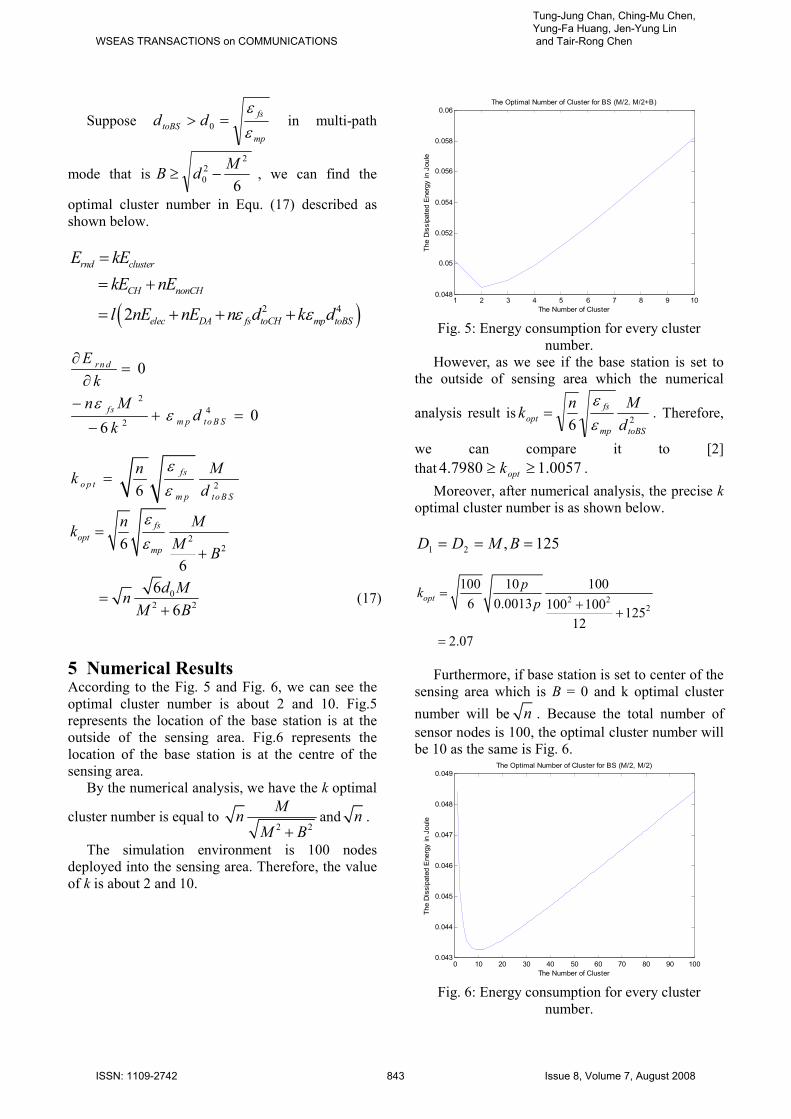
5 Numerical Results According to the Fig. 5 and Fig. 6, we can see the
optimal cluster number is about 2 and 10. Fig.5
represents the location of the base station is at the
outside of the sensing area. Fig.6 represents the
location of the base station is at the centre of the
sensing area.
By the numerical analysis, we have the k optimal
cluster number is equal to 2 2
Mn
M B+and n .
The simulation environment is 100 nodes
deployed into the sensing area. Therefore, the value
of k is about 2 and 10.
1 2 3 4 5 6 7 8 9 100.048
0.05
0.052
0.054
0.056
0.058
0.06The Optimal Number of Cluster for BS (M/2, M/2+B)
The Number of Cluster
The Dissipated Energy in Joule
Fig. 5: Energy consumption for every cluster
number.
However, as we see if the base station is set to
the outside of sensing area which the numerical
analysis result is26 toBSmp
fs
optd
Mnk
ε
ε= . Therefore,
we can compare it to [2]
that 0057.17980.4 ≥≥ optk .
Moreover, after numerical analysis, the precise k
optimal cluster number is as shown below.
125,21 === BMDD
2 22
100 10 100
6 0.0013 100 100125
12
2.07
opt
pk
p=
++
=
Furthermore, if base station is set to center of the
sensing area which is B = 0 and k optimal cluster
number will be n . Because the total number of
sensor nodes is 100, the optimal cluster number will
be 10 as the same is Fig. 6.
0 10 20 30 40 50 60 70 80 90 1000.043
0.044
0.045
0.046
0.047
0.048
0.049The Optimal Number of Cluster for BS (M/2, M/2)
The Number of Cluster
The Dissipated Energy in Joule
Fig. 6: Energy consumption for every cluster
number.
WSEAS TRANSACTIONS on COMMUNICATIONS
Tung-Jung Chan, Ching-Mu Chen, Yung-Fa Huang, Jen-Yung Lin and Tair-Rong Chen
ISSN: 1109-2742 843 Issue 8, Volume 7, August 2008

6 Simulation Results In order to have better simulation result, the
simulation tool, Matlab, is used as simulator. In the
simulation environment, 100 sensor nodes are
randomly deployed as shown in Fig. 7.
Fig. 7: 100 sensor nodes are randomly deployed.
Fig. 8 shows the formation of clusters and how
many nodes are still alive there. “o” denotes sensor
node is still alive where as “.” denotes node is no
longer alive and ‘*’ denotes cluster head. Also,
sensor node’s colour stands for which node belongs
to which cluster.
Fig.8: Cluster formation and cluster head selection.
By evaluating 310 rounds in Fig. 9 and 1200
rounds in Fig. 10, numbers of cluster head from
both figures are different and nodes’ number
belongs to each cluster from these two figures are
also different. Therefore, by Fig. 10, it shows those
sensor nodes closer to the base station will be run
out of energy quickly.
Fig. 9: Sensor nodes are still alive after 310 rounds.
Fig. 10 Sensor nodes are still alive after 310 rounds.
As the base station is set at the centre of the
sensing area, Fig. 10 shows how many nodes are
still alive and how many nodes are no longer alive.
It is obvious that energy usage for nodes far away
from the base station is less than those nodes closer
to the base station. Therefore, the probability and
cluster formation need to be adjusted in order to
have the dissipated energy evenly.
Fig. 11 shows that total packets are transmitted
from cluster head to the base station. Before the
first node runs out of the energy, packets sent from
cluster head to base station are the same. However,
once first node starts running out of its energy, the
total amount of packets to transmit the data back to
the base station would be down very fast.
WSEAS TRANSACTIONS on COMMUNICATIONS
Tung-Jung Chan, Ching-Mu Chen, Yung-Fa Huang, Jen-Yung Lin and Tair-Rong Chen
ISSN: 1109-2742 844 Issue 8, Volume 7, August 2008

0 200 400 600 800 1000 1200 1400 1600 18000
10
20
30
40
50
60
70
80
90r:pkt2bs g:pkt2ch
rounds
packets(:4000 bits/packet)
Fig. 11: Total packets are transmitted from cluster
head to base station.
However, LEACH with pre-determined variable
p =0.05 is applied as shown in the Fig. 12.
According to the LEACH architecture, the k optimal
cluster number is around from 1 to 5. It is obvious
that LEACH with the proposed fixed optimal cluster
number = 5 has the better performance.
Fig. 12: Comparison between LEACH (p=0.05) and
LEACH with fixed optimal cluster head = 5.
7 Conclusion This paper reveals the proposed fixed optimal
cluster number with random and probability in the
clustering-based scheme has the better performance.
The numerical analysis shows the optimal cluster
number is equal to 10 around as the base station is
set to the centre of the sensing area and the optimal
cluster number is equal to 2 for the outside of the
sensing area. Using the proposed fixed optimal
cluster number for clusters and cluster heads
especially for the architecture of LEACH, the
simulation results show the entire network can be
extended very well which means the proposed
scheme in this paper has much better performance
compared to the LEACH architecture in the ad-hoc
WSN.
References:
[1] A. Willig, "Recent and Emerging Topics in
Wireless Industrial Communications: A
Selection", IEEE Transactions on Industrial
Informatics, Vol. 4, No. 2, May 2008.
[2] D. Culler, D. Estrin and M. Srivastava,
"Overview of sensor networks", IEEE
Computer, Vol. 37, Issue 8, pp. 41- 49, Aug.
2004.
[3] I. F. Akyildiz, W. Su, Y.Sankarasubramaniam,
E. Cayirci, "Wireless sensor network: a survey",
Computer Networks, Vol. 38, pp. 393-422,
2002.
[4] W.R. Heinzelman, A.P. Chandrakasan, and H.
Balakrishnan,"Energy-EfficientCommunication
Protocol for Wireless Microsensor Networks",
Proc. 33rd Hawaii Int’l. Conf. Sys. Sci., Jan.
2000.
[5] A. Ahmed A., and M. Younis, "A survey on
clustering algorithms for wireless sensor
networks", Elsevier: computer communications,
2007.
[6] W.B. Heinzelman, A.P. Chandrakasan, and H.
Balakrishnan,"An Application-Specific
Protocol Architecture for Wireless Microsensor
Networksv, IEEE Trans. Wireless Commun.,
vol. 1, no. 4, Oct. 2002, pp. 660–70.
[7] O. Younis and S. Fahmy,"HEED: a hybrid,
energy-efficient, distributed clustering
approach for ad hoc sensor networks", IEEE
Trans. on Mobile Computing, pp. 660-669,
2004
[8] S.D. Muruganathan, D.C.F. Ma, R.I. Bhasin,
and A.O. Fapojuwo, "A Centralized Energy-
Efficient Routing Protocol for Wireless Sensor
Networks", IEEE Radio Communication, 2005
[9] Y.-R. Tsai, "Coverage-Preserving Routing
Protocols for Randomly Distributed Wireless
Sensor Networks", IEEE Trans. Wireless on
Wireless Commun., Vol. 6, No. 4, Apr. 2007.
[10] J. Zhu and S. Papavassiliou, "On the energy-
efficient organization and the lifetime of multi-
hop sensor networks", IEEE Commun. Letters,
Vol. 7, No. 11, pp. 537-539, Nov. 2003.
WSEAS TRANSACTIONS on COMMUNICATIONS
Tung-Jung Chan, Ching-Mu Chen, Yung-Fa Huang, Jen-Yung Lin and Tair-Rong Chen
ISSN: 1109-2742 845 Issue 8, Volume 7, August 2008

[11] V. Raghunathan et al.,"Energy-Aware Wireless
Microsensor Networks", IEEE Sig. Proc. Mag.,
vol. 1, no. 2, Mar. 2002, pp. 40–50.
[12] C. Schurgers and M.B. Srivastava, "Energy
efficient routing in wireless sensor networks",
IEEE Military Comm. Conf., Vol. 1, pp. 357-
361, Oct. 2001.
[13] V. Raghunathan, C. Schurgers and S. Park and
M. B. Srivastava, "Energy-aware wireless
microsensor networks", IEEE Signal
Processing Magazine, Vol. 19, No. 2, pp. 40-
50, March 2002.
[14] M. Younis, M. Youssef, K. Arisha, "Energy-
aware routing in cluster-based sensor
networks", 10th IEEE International Symposium
on Modeling, Analysis and Simulation of
Computer and Telecommunications Systems,
pp. 129 – 136, 2002.
[15] Song Ci, Mohsen Guizani and Hamid Sharif,
"Adaptive clustering in wireless sensor
networks by mining sensor energy data",
Elsevier: computer communications, 2007.
[16] N. Pantazis, D. Kandris, “Power Control
Schemes in Wireless Sensor Networks”,
WSEAS Transactions on Communications,
Issue X, Vol. 4, October 2005, pp. 1100–1107.
[17] Y. Yin, J. Shi, Y. Li and P. Zhang, "Cluster
Head Selection Using Analytical Hierarchy
Process For Wireless Sensor Networks", the
17th Annual IEEE International Symposium on
Personal, Indoor and Mobile Radio comm.,
PIMRC'06.
[18] T. Kang, J. Yun, H. Lee, I. Lee, H. KIM, B.
Lee, B. Lee and K. Han, "A Clustering Method
for Energy Efficient Routing in Wireless
Sensor Networks", Proc. of the 6th WSEAS Int.
Conf. on Electronics, Hardware, Wireless and
Optical Comm., 2007.
[19] J. Y. Yu and P. H. J, "A Survey of Clustering
Schemes for Mobile Ad Hoc Networks", IEEE
Communications Surveys & Tutorials, 2005.
[20] M. Veyseh, B. W. Wei, and N. F. Mir,
"Clustering and Synchronization Protocol in a
Wireless Sensor Networks", WSEAS
Transactions in Communications, 2006.
[21] M. Cardei and J. Wu, "Energy-Efficient
Coverage Problems in Wireless Ad Hoc Sensor
Networks", Computer Communications, vol. 29,
no. 4, Feb. 2006, pp. 413-420.
[22] Gracanin, D. Eltoweissy, M. Olariu, S. Wadaa,
"On modeling wireless sensor networks,” A.
Parallel and Distributed Processing Symposium,
2004.
[23] R. M. Patrikar and S. G. Akojwar, " Neural
Network Based Classification Techniques For
Wireless Sensor Network with Cooperative
Routing", 12th WSEAS International
Conference on Communications.
[24] C. Sevgi and A. Koc¸yi˜git, "On determining
cluster size of randomly deployed
heterogeneous WSNs", IEEE Communications
Letters, Vol. 12, No. 4, April 2008.
WSEAS TRANSACTIONS on COMMUNICATIONS
Tung-Jung Chan, Ching-Mu Chen, Yung-Fa Huang, Jen-Yung Lin and Tair-Rong Chen
ISSN: 1109-2742 846 Issue 8, Volume 7, August 2008


![A modified cluster-head selection algorithm in …...data transmission [8]. In response to these problems, this paper presents a modified cluster-head selection algorithm based on](https://img.pdfslide.net/doc/110x75/5f081b087e708231d4205d43/a-modified-cluster-head-selection-algorithm-in-data-transmission-8-in-response.jpg)


![Research Article An Efficient Cluster Head Selection ...downloads.hindawi.com/journals/ijdsn/2015/794518.pdf · and cluster head selection [ ]. Although LEACH protocol can e ectively](https://img.pdfslide.net/doc/110x75/5f03b0557e708231d40a4928/research-article-an-efficient-cluster-head-selection-and-cluster-head-selection.jpg)