Embed Size (px)
Citation preview
Optimal Control and Applications inOperations Research and Economics
Alan Zinober
Sheffield University
May 2008
A Deep Question
Whom will you support tonight?
Manchester United or Chelsea

A Deep Question
Whom will you support tonight?
Manchester United or Chelsea

A Deep Question
Whom will you support tonight?
Manchester United or Chelsea
Overview
1 Brachystochrone problem
graphical descriptionderivation of dynamical equations
2 This problem was posed in a competition by Jean Bernoulliin 1696. Early solutions May 1697
Johann’s elder brother JakobLeibnizNewtonl’HôpitalTschirnhaus
3 The Calculus of Variations c17504 Pontryagin’s Maximum Principle 19615 Differential geometry techniques post 1980
Overview
1 Brachystochrone problem
graphical descriptionderivation of dynamical equations
2 This problem was posed in a competition by Jean Bernoulliin 1696.
Early solutions May 1697
Johann’s elder brother JakobLeibnizNewtonl’HôpitalTschirnhaus
3 The Calculus of Variations c17504 Pontryagin’s Maximum Principle 19615 Differential geometry techniques post 1980
Overview
1 Brachystochrone problem
graphical descriptionderivation of dynamical equations
2 This problem was posed in a competition by Jean Bernoulliin 1696. Early solutions May 1697
Johann’s elder brother JakobLeibnizNewtonl’HôpitalTschirnhaus
3 The Calculus of Variations c17504 Pontryagin’s Maximum Principle 19615 Differential geometry techniques post 1980
Overview
1 Brachystochrone problem
graphical descriptionderivation of dynamical equations
2 This problem was posed in a competition by Jean Bernoulliin 1696. Early solutions May 1697
Johann’s elder brother JakobLeibnizNewtonl’HôpitalTschirnhaus
3 The Calculus of Variations c1750
4 Pontryagin’s Maximum Principle 19615 Differential geometry techniques post 1980
Overview
1 Brachystochrone problem
graphical descriptionderivation of dynamical equations
2 This problem was posed in a competition by Jean Bernoulliin 1696. Early solutions May 1697
Johann’s elder brother JakobLeibnizNewtonl’HôpitalTschirnhaus
3 The Calculus of Variations c17504 Pontryagin’s Maximum Principle 1961
5 Differential geometry techniques post 1980
Overview
1 Brachystochrone problem
graphical descriptionderivation of dynamical equations
2 This problem was posed in a competition by Jean Bernoulliin 1696. Early solutions May 1697
Johann’s elder brother JakobLeibnizNewtonl’HôpitalTschirnhaus
3 The Calculus of Variations c17504 Pontryagin’s Maximum Principle 19615 Differential geometry techniques post 1980
Some Interesting OR and Economic Applications
Optimal capital spending
Optimal reservoir control
Optimal Production subject to Piecewise ContinuousRoyalty Payment Obligations
Optimal maintenance and replacement policy
Optimal drug bust strategy
Optimal study for examinations
Optimal slide presentation
Historical Development
The first optimisation result ever discovered must have been thestatement that the shortest path joining two points is a straightline segment.
The isoperimetric problem is the problem of
finding, amongst all simple closed plane curves of a given fixedlength, one that encloses the largest possible area. The circle
is the shape that encloses maximum area for a given length ofperimeter. It was not until the eighteenth century that a
systematic theory, the Calculus of Variations, began to emerge.
Historical Development
The first optimisation result ever discovered must have been thestatement that the shortest path joining two points is a straightline segment. The isoperimetric problem is the problem of
finding, amongst all simple closed plane curves of a given fixedlength, one that encloses the largest possible area.
The circle
is the shape that encloses maximum area for a given length ofperimeter. It was not until the eighteenth century that a
systematic theory, the Calculus of Variations, began to emerge.
Historical Development
The first optimisation result ever discovered must have been thestatement that the shortest path joining two points is a straightline segment. The isoperimetric problem is the problem of
finding, amongst all simple closed plane curves of a given fixedlength, one that encloses the largest possible area. The circle
is the shape that encloses maximum area for a given length ofperimeter.
It was not until the eighteenth century that a
systematic theory, the Calculus of Variations, began to emerge.
Historical Development
The first optimisation result ever discovered must have been thestatement that the shortest path joining two points is a straightline segment. The isoperimetric problem is the problem of
finding, amongst all simple closed plane curves of a given fixedlength, one that encloses the largest possible area. The circle
is the shape that encloses maximum area for a given length ofperimeter. It was not until the eighteenth century that a
systematic theory, the Calculus of Variations, began to emerge.
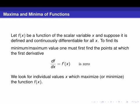
Maxima and Minima of Functions
Let f (x) be a function of the scalar variable x and suppose it isdefined and continuously differentiable for all x . To find its
minimum/maximum value one must first find the points at whichthe first derivative
dfdx
= f ′(x) is zero
We look for individual values x which maximize (or minimize)the function f (x).
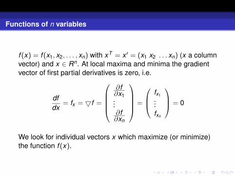
Functions of n variables
f (x) = f (x1, x2, . . . , xn) with xT = x ′ = (x1 x2 . . . xn) (x a columnvector) and x ∈ Rn. At local maxima and minima the gradientvector of first partial derivatives is zero, i.e.
dfdx
= fx = 5f =
∂f∂x1...∂f∂xn
=
fx1...fxn
= 0
We look for individual vectors x which maximize (or minimize)the function f (x).
Brachystochrone Problem
This was posed in a competition by Jean Bernoulli in 1696.
The problem involves a bead sliding under gravity along asmooth wire joining two fixed points A and B (not directly belowA).
What shape should the wire have so that the bead, whenreleased from rest at A, slides under gravity from A to B inminimum time T?
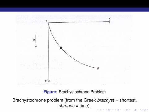
Figure: Brachystochrone Problem
Brachystochrone problem (from the Greek brachyst = shortest,chronos = time).
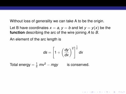
Without loss of generality we can take A to be the origin.
Let B have coordinates x = a, y = b and let y = y(x) be thefunction describing the arc of the wire joining A to B.
An element of the arc length is
ds =
[1 +
(dydx
)2] 1
2
dx
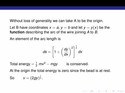
Total energy = 12 mv2 −mgy is conserved.
At the origin the total energy is zero since the bead is at rest.
So v = (2gy)12 .
Without loss of generality we can take A to be the origin.
Let B have coordinates x = a, y = b and let y = y(x) be thefunction describing the arc of the wire joining A to B.
An element of the arc length is
ds =
[1 +
(dydx
)2] 1
2
dx
Total energy = 12 mv2 −mgy is conserved.
At the origin the total energy is zero since the bead is at rest.
So v = (2gy)12 .
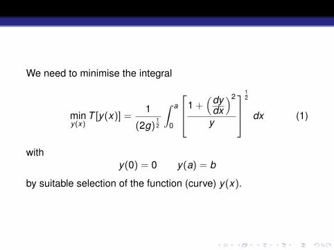
We need to minimise the integral
miny(x)
T [y(x)] =1
(2g)12
∫ a
0
1 +(dy
dx
)2
y
12
dx (1)
withy(0) = 0 y(a) = b
by suitable selection of the function (curve) y(x).
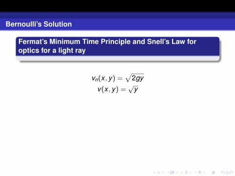
Bernoulli’s Solution
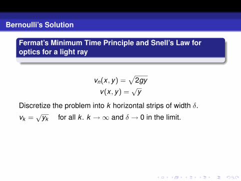
Fermat’s Minimum Time Principle and Snell’s Law foroptics for a light ray
vn(x , y) =√
2gy
v(x , y) =√
y
Discretize the problem into k horizontal strips of width δ.
vk =√
yk for all k . k →∞ and δ → 0 in the limit.
Snell′s Lawsin θ1
v1=
sin θ2
v2
Sosin θk
vk=
sin θk√yk
= constant
Bernoulli’s Solution
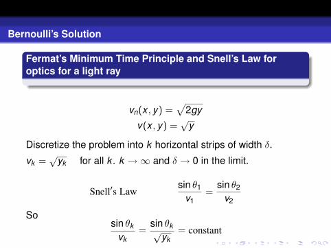
Fermat’s Minimum Time Principle and Snell’s Law foroptics for a light ray
vn(x , y) =√
2gy
v(x , y) =√
y
Discretize the problem into k horizontal strips of width δ.
vk =√
yk for all k . k →∞ and δ → 0 in the limit.
Snell′s Lawsin θ1
v1=
sin θ2
v2
Sosin θk
vk=
sin θk√yk
= constant
Bernoulli’s Solution
Fermat’s Minimum Time Principle and Snell’s Law foroptics for a light ray
vn(x , y) =√
2gy
v(x , y) =√
y
Discretize the problem into k horizontal strips of width δ.
vk =√
yk for all k . k →∞ and δ → 0 in the limit.
Snell′s Lawsin θ1
v1=
sin θ2
v2
Sosin θk
vk=
sin θk√yk
= constant
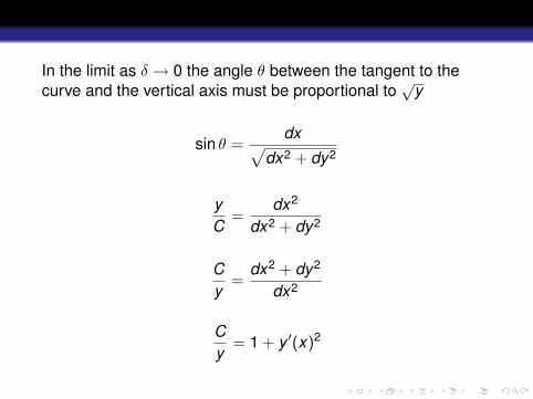
In the limit as δ → 0 the angle θ between the tangent to thecurve and the vertical axis must be proportional to
√y
sin θ =dx√
dx2 + dy2
yC
=dx2
dx2 + dy2
Cy
=dx2 + dy2
dx2
Cy
= 1 + y ′(x)2
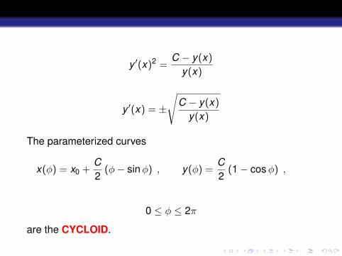
y ′(x)2 =C − y(x)
y(x)
y ′(x) = ±
√C − y(x)
y(x)
The parameterized curves
x(φ) = x0 +C2
(φ− sin φ) , y(φ) =C2
(1− cos φ) ,
0 ≤ φ ≤ 2π
are the CYCLOID.
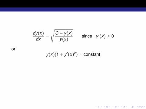
dy(x)
dx=
√C − y(x)
y(x)since y ′(x) ≥ 0
ory(x)(1 + y ′(x)2) = constant
For any constant y > 0 y = y (∗) is a solution
corresponding to C = y withdydx
= 0.
So one could theoretically have the cycloid solution up to φ = πwith constant paths thereafter.
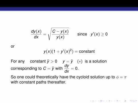
dy(x)
dx=
√C − y(x)
y(x)since y ′(x) ≥ 0
ory(x)(1 + y ′(x)2) = constant
For any constant y > 0 y = y (∗) is a solution
corresponding to C = y withdydx
= 0.
So one could theoretically have the cycloid solution up to φ = πwith constant paths thereafter.
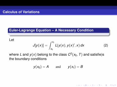
Calculus of Variations
Euler-Lagrange Equation – A Necessary Condition
Let
J[y(x)] =
∫ xf
x0
L(y(x), y(x)′, x) dx (2)
where L and y(x) belong to the class C2(x0, T ) and satisfie)sthe boundary conditions
y(x0) = A and y(xf ) = B
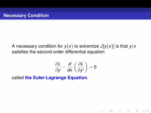
Necessary Condition
A necessary condition for y(x) to extremize J[y(x)] is that y(xsatisfies the second-order differential equation
∂L∂y
− ddx
(∂L∂y ′
)= 0
called the Euler-Lagrange Equation.
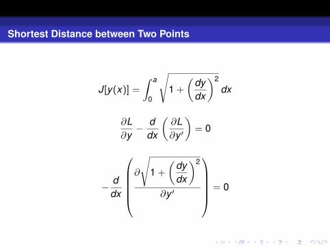
Shortest Distance between Two Points
J[y(x)] =
∫ a
0
√1 +
(dydx
)2
dx
∂L∂y
− ddx
(∂L∂y ′
)= 0
− ddx
∂
√1 +
(dydx
)2
∂y ′
= 0
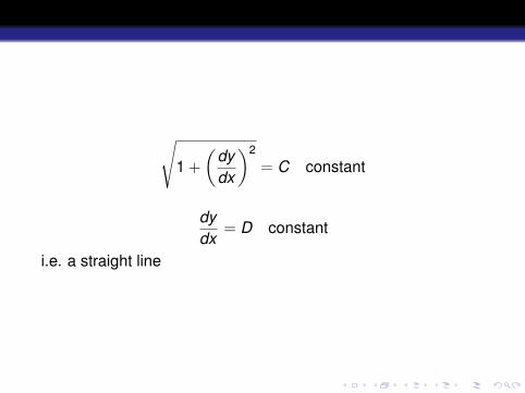
√1 +
(dydx
)2
= C constant
dydx
= D constant
i.e. a straight line
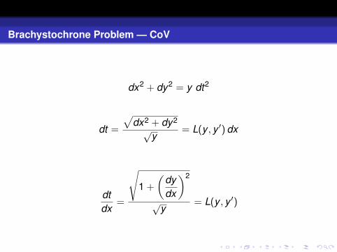
Brachystochrone Problem — CoV
dx2 + dy2 = y dt2
dt =
√dx2 + dy2√
y= L(y , y ′) dx
dtdx
=
√1 +
(dydx
)2
√y
= L(y , y ′)
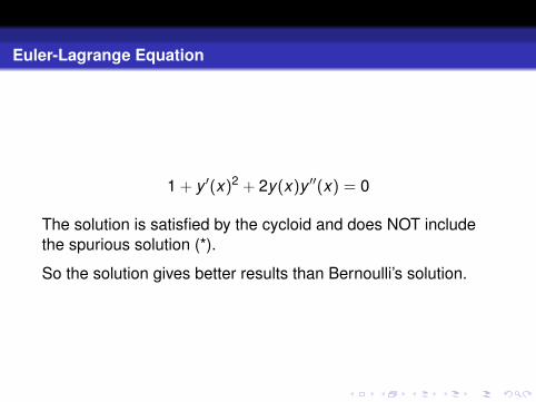
Euler-Lagrange Equation
1 + y ′(x)2 + 2y(x)y ′′(x) = 0
The solution is satisfied by the cycloid and does NOT includethe spurious solution (*).
So the solution gives better results than Bernoulli’s solution.
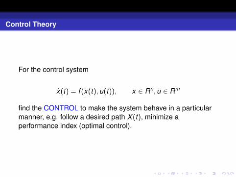
Control Theory
For the control system
x(t) = f (x(t), u(t)), x ∈ Rn, u ∈ Rm
find the CONTROL to make the system behave in a particularmanner, e.g. follow a desired path X (t), minimize aperformance index (optimal control).
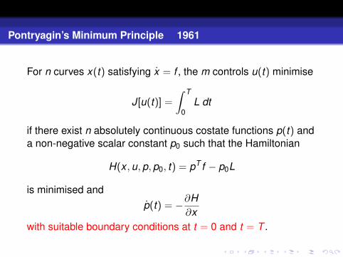
Pontryagin’s Minimum Principle 1961
For n curves x(t) satisfying x = f , the m controls u(t) minimise
J[u(t)] =
∫ T
0L dt
if there exist n absolutely continuous costate functions p(t) anda non-negative scalar constant p0 such that the Hamiltonian
H(x , u, p, p0, t) = pT f − p0L
is minimised andp(t) = −∂H
∂xwith suitable boundary conditions at t = 0 and t = T .
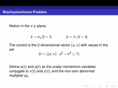
Brachystochrone Problem
Motion in the x-y plane.
x = u√
y = f1 y = v√
y = f2
The control is the 2-dimensional vector (u, v) with values in theset
U = {(u, v) : u2 + v2 ≤ 1}
Define p(t) and q(t) as the scalar momentum variablesconjugate to x(t) and y(t), and the non-zero abnormalmultiplier p0.
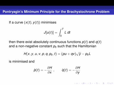
Pontryagin’s Minimum Principle for the Brachystochrone Problem
If a curve (x(t), y(t)) minimises
J[u(t)] =
∫ T
0L dt
then there exist absolutely continuous functions p(t) and q(t)and a non-negative constant p0 such that the Hamiltonian
H(x , y , u, v , p, q, p0, t) = (pu + qv)√
y − p0L
is minimised and
p(t) = −∂H∂x
, q(t) = −∂H∂y
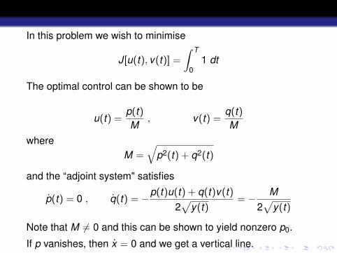
In this problem we wish to minimise
J[u(t), v(t)] =
∫ T
01 dt
The optimal control can be shown to be
u(t) =p(t)M
, v(t) =q(t)M
whereM =
√p2(t) + q2(t)
and the “adjoint system" satisfies
p(t) = 0 , q(t) = −p(t)u(t) + q(t)v(t)2√
y(t)= − M
2√
y(t)
Note that M 6= 0 and this can be shown to yield nonzero p0.
If p vanishes, then x = 0 and we get a vertical line.
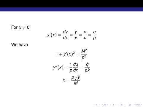
For x 6= 0.
y ′(x) =dydx
=yx
=vu
=qp
We have
1 + y ′(x)2 =M2
p2
y ′′(x) =1p
dqdx
=q
px
x =p√
yM
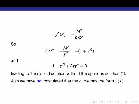
y ′′(x) = − M2
2yp2
So
2yy ′′ = −M2
p2 = −(1 + y ′2)
and1 + y ′2 + 2yy ′′ = 0
leading to the cycloid solution without the spurious solution (*).
Also we have not postulated that the curve has the form y(x).
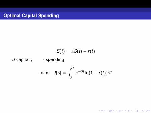
Optimal Capital Spending
S(t) = αS(t)− r(t)
S capital ; r spending
max J[u] =
∫ T
0e−βt ln(1 + r(t))dt
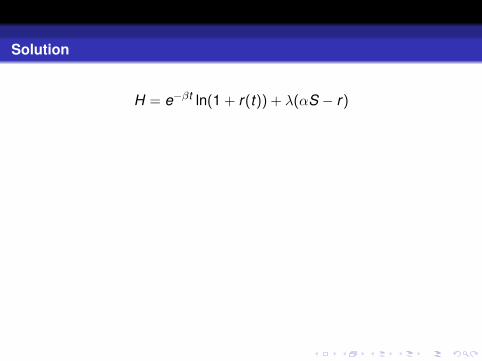
Solution
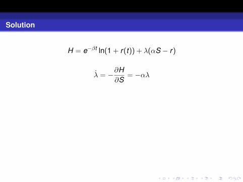
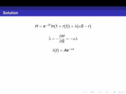
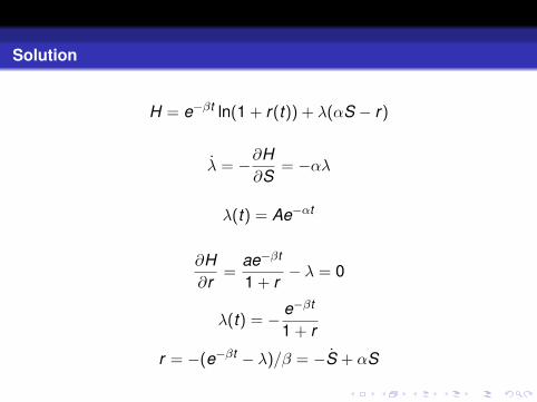
H = e−βt ln(1 + r(t)) + λ(αS − r)
λ = −∂H∂S
= −αλ
λ(t) = Ae−αt
∂H∂r
=ae−βt
1 + r− λ = 0
λ(t) = − e−βt
1 + r
r = −(e−βt − λ)/β = −S + αS
Solution
H = e−βt ln(1 + r(t)) + λ(αS − r)
λ = −∂H∂S
= −αλ
λ(t) = Ae−αt
∂H∂r
=ae−βt
1 + r− λ = 0
λ(t) = − e−βt
1 + r
r = −(e−βt − λ)/β = −S + αS
Solution
H = e−βt ln(1 + r(t)) + λ(αS − r)
λ = −∂H∂S
= −αλ
λ(t) = Ae−αt
∂H∂r
=ae−βt
1 + r− λ = 0
λ(t) = − e−βt
1 + r
r = −(e−βt − λ)/β = −S + αS
Solution
H = e−βt ln(1 + r(t)) + λ(αS − r)
λ = −∂H∂S
= −αλ
λ(t) = Ae−αt
∂H∂r
=ae−βt
1 + r− λ = 0
λ(t) = − e−βt
1 + r
r = −(e−βt − λ)/β = −S + αS
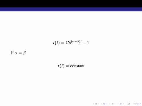
r(t) = Ce(α−β)t − 1
If α = β
r(t) = constant
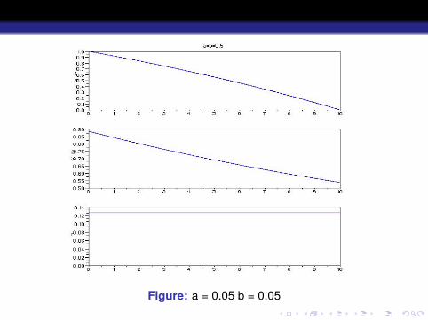
Figure: a = 0.05 b = 0.05
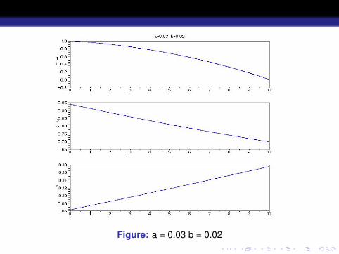
Figure: a = 0.03 b = 0.02
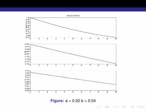
Figure: a = 0.02 b = 0.04
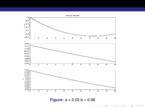
Figure: a = 0.02 b = 0.06
Optimal Production subject to Piecewise Continuous RoyaltyPayment Obligations
with Kim Kaivanto (2008)
A standard feature of the theory of the firm is that a profitmaximising firm facing a downward sloping demand curvereacts to an increase in marginal cost by reducing output andincreasing price.
In this context, it is well understood that a requirement to pay aflat-rate royalty on sales has just this effect of increasingmarginal cost and thereby decreasing output whilesimultaneously increasing price.
However the effect of permitting the royalty to take on moregeneral forms has remained unaddressed to date.
Here we investigate very briefly the effect of piecewise linearcumulative royalty schedules on the optimal intertemporalproduction policy.
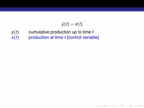
y(t) = x(t)
y(t) cumulative production up to time tx(t) production at time t [control variable]
Maximise by selection of optimal x(t)
J[x(t)] =
∫ T
0{[a(t)x−α − (m0 + ρ + c0e−λy )}x(t)e−rt ] dt
=
∫ T
0g(y , x , t) dt
a(t)x−α demand curve and r is the discount ratem0 + c0e−λy learning curve (unit cost for producing one unitof output)ρ(x(t), y(t), t)x(t) total royalty paid at time t
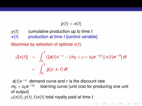
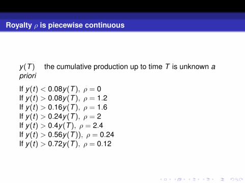
Royalty ρ is piecewise continuous
y(T ) the cumulative production up to time T is unknown apriori
If y(t) < 0.08y(T ), ρ = 0If y(t) > 0.08y(T ), ρ = 1.2If y(t) > 0.16y(T ), ρ = 1.6If y(t) > 0.24y(T ), ρ = 2If y(t) > 0.4y(T ), ρ = 2.4If y(t) > 0.56y(T )), ρ = 0.24If y(t) > 0.72y(T ), ρ = 0.12
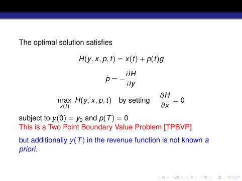
The optimal solution satisfies
H(y , x , p, t) = x(t) + p(t)g
p = −∂H∂y
maxx(t)
H(y , x , p, t) by setting∂H∂x
= 0
subject to y(0) = y0 and p(T ) = 0This is a Two Point Boundary Value Problem [TPBVP]
but additionally y(T ) in the revenue function is not known apriori.
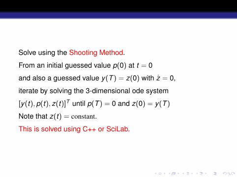
Solve using the Shooting Method.
From an initial guessed value p(0) at t = 0
and also a guessed value y(T ) = z(0) with z = 0,
iterate by solving the 3-dimensional ode system
[y(t), p(t), z(t)]T until p(T ) = 0 and z(0) = y(T )
Note that z(t) = constant.
This is solved using C++ or SciLab.
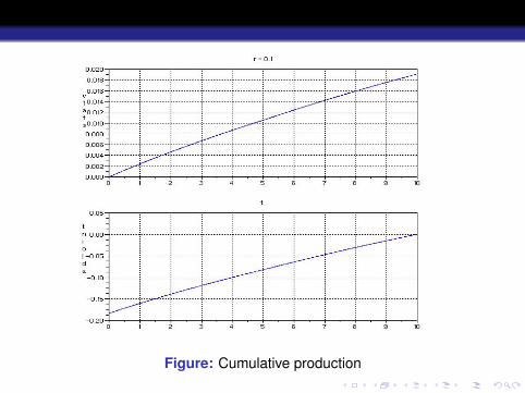
Figure: Cumulative production
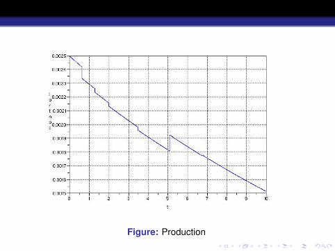
Figure: Production
Optimal Maintenance and Replacement Policy
How long should one keep a motor car, knowing that withoutmaintenance expenditure u(t) the car will deteriorate at a rateδ. Beyond a certain age the car will not be worthwhile to repair.
x(t) = −δx(t) + u(t)g(t)
where g(t) is the maintenance effectiveness function. Onewishes to maximise
J[u(t)] =
∫ T
0{wx(t)− u(t)e−rt}dt + x(T )e−rt
where w > 0 and the discount factor r > 0 and
0 ≤ u(t) ≤ M , M > 0
T and x(T ) are free.
Optimal Crackdown on Illicit Drug Markets [Baveja, Feichtinger,Hartl et al]
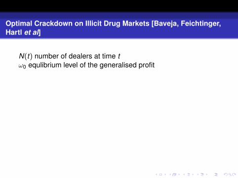
N(t) number of dealers at time tω0 equlibrium level of the generalised profit
If generalised profit > ω0 dealers enterπ(t) generalised profit per unit of sales in the marketαNβ = number of sales per day with N dealersE(t) enforcement effort with crackdown at time tgeneralised net profit with per dealer cost of enforcement isπαNβ/N −
(EN
)γ
N = c1
[παNβ−1 −
(EN
)γ
− ω0
]where c1 is the speed of adjustment parameter
Optimal Crackdown on Illicit Drug Markets [Baveja, Feichtinger,Hartl et al]
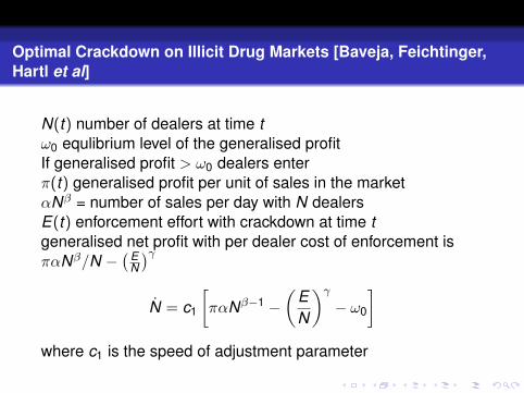
N(t) number of dealers at time tω0 equlibrium level of the generalised profitIf generalised profit > ω0 dealers enterπ(t) generalised profit per unit of sales in the marketαNβ = number of sales per day with N dealersE(t) enforcement effort with crackdown at time tgeneralised net profit with per dealer cost of enforcement isπαNβ/N −
(EN
)γ
N = c1
[παNβ−1 −
(EN
)γ
− ω0
]where c1 is the speed of adjustment parameter
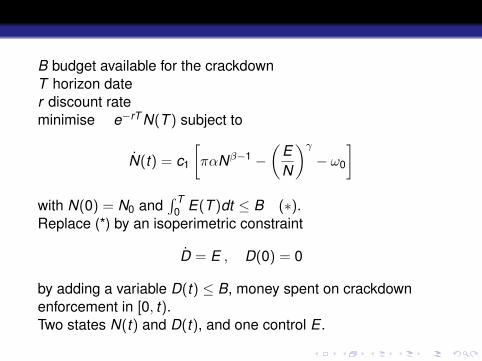
B budget available for the crackdownT horizon dater discount rateminimise e−rT N(T ) subject to
N(t) = c1
[παNβ−1 −
(EN
)γ
− ω0
]with N(0) = N0 and
∫ T0 E(T )dt ≤ B (∗).
Replace (*) by an isoperimetric constraint
D = E , D(0) = 0
by adding a variable D(t) ≤ B, money spent on crackdownenforcement in [0, t).Two states N(t) and D(t), and one control E .
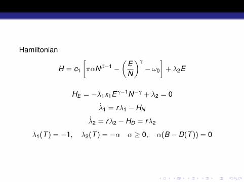
Hamiltonian
H = c1
[παNβ−1 −
(EN
)γ
− ω0
]+ λ2E
HE = −λ1x1Eγ−1N−γ + λ2 = 0
λ1 = rλ1 − HN
λ2 = rλ2 − HD = rλ2
λ1(T ) = −1, λ2(T ) = −α α ≥ 0, α(B − D(T )) = 0
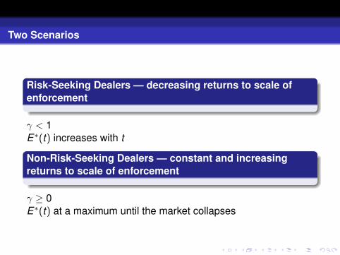
Two Scenarios
Risk-Seeking Dealers — decreasing returns to scale ofenforcement
γ < 1E∗(t) increases with t
Non-Risk-Seeking Dealers — constant and increasingreturns to scale of enforcement
γ ≥ 0E∗(t) at a maximum until the market collapses
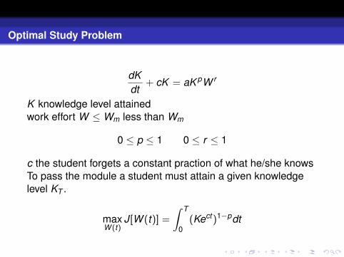
Optimal Study Problem
dKdt
+ cK = aK pW r
K knowledge level attainedwork effort W ≤ Wm less than Wm
0 ≤ p ≤ 1 0 ≤ r ≤ 1
c the student forgets a constant praction of what he/she knowsTo pass the module a student must attain a given knowledgelevel KT .
maxW (t)
J[W (t)] =
∫ T
0(Kect)1−pdt
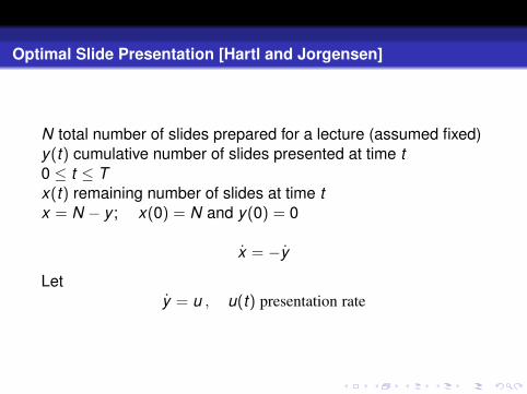
Optimal Slide Presentation [Hartl and Jorgensen]
N total number of slides prepared for a lecture (assumed fixed)y(t) cumulative number of slides presented at time t0 ≤ t ≤ Tx(t) remaining number of slides at time tx = N − y ; x(0) = N and y(0) = 0
x = −y
Lety = u , u(t) presentation rate
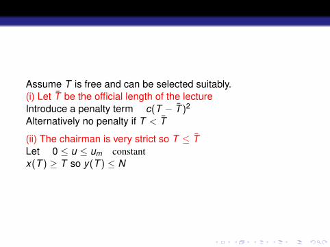
Assume T is free and can be selected suitably.(i) Let T be the official length of the lectureIntroduce a penalty term c(T − T )2
Alternatively no penalty if T < T
(ii) The chairman is very strict so T ≤ TLet 0 ≤ u ≤ um constantx(T ) ≥ T so y(T ) ≤ N
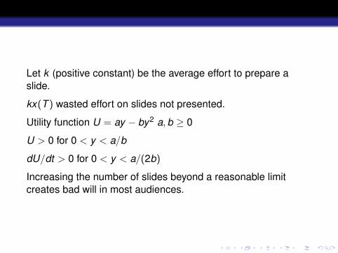
Let k (positive constant) be the average effort to prepare aslide.
kx(T ) wasted effort on slides not presented.
Utility function U = ay − by2 a, b ≥ 0
U > 0 for 0 < y < a/b
dU/dt > 0 for 0 < y < a/(2b)
Increasing the number of slides beyond a reasonable limitcreates bad will in most audiences.
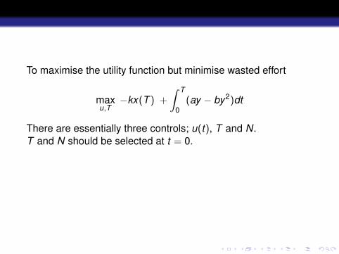
To maximise the utility function but minimise wasted effort
maxu,T
−kx(T ) +
∫ T
0(ay − by2)dt
There are essentially three controls; u(t), T and N.T and N should be selected at t = 0.
It is convenient to set N(0) as a degenerate state variable
N(0) free and N(T ) free and N = 0
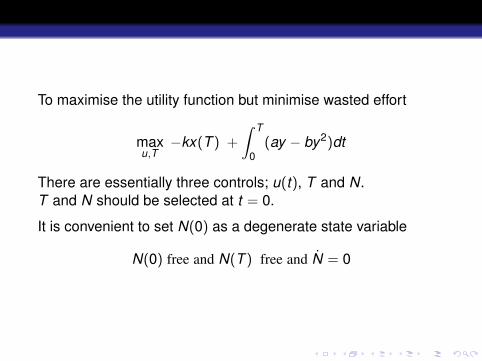
To maximise the utility function but minimise wasted effort
maxu,T
−kx(T ) +
∫ T
0(ay − by2)dt
There are essentially three controls; u(t), T and N.T and N should be selected at t = 0.
It is convenient to set N(0) as a degenerate state variable
N(0) free and N(T ) free and N = 0
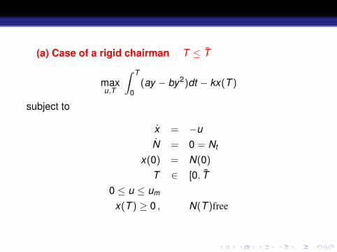
(a) Case of a rigid chairman T ≤ T
maxu,T
∫ T
0(ay − by2)dt − kx(T )
subject to
x = −uN = 0 = Nt
x(0) = N(0)
T ∈ [0, T0 ≤ u ≤ um
x(T ) ≥ 0 , N(T )free
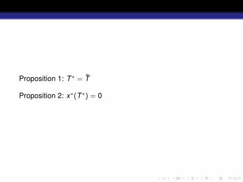
Proposition 1: T ∗ = T
Proposition 2: x∗(T ∗) = 0
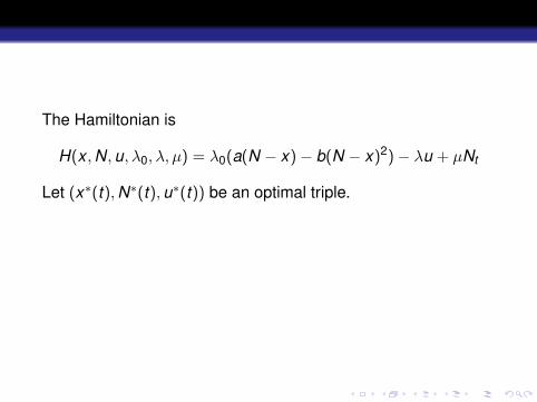
The Hamiltonian is
H(x , N, u, λ0, λ, µ) = λ0(a(N − x)− b(N − x)2)− λu + µNt
Let (x∗(t), N∗(t), u∗(t)) be an optimal triple.
There exists a constant λ0 ≥ 0.Let λ0 = 1 say.There exist piecewise continuously differentiable costates λ(t),µ(t) and constant multipliers α, β such that (λ0, λ, µ, α, β) 6= 0except at discontinuous points of u∗
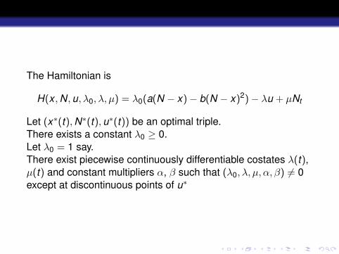
The Hamiltonian is
H(x , N, u, λ0, λ, µ) = λ0(a(N − x)− b(N − x)2)− λu + µNt
Let (x∗(t), N∗(t), u∗(t)) be an optimal triple.There exists a constant λ0 ≥ 0.Let λ0 = 1 say.There exist piecewise continuously differentiable costates λ(t),µ(t) and constant multipliers α, β such that (λ0, λ, µ, α, β) 6= 0except at discontinuous points of u∗
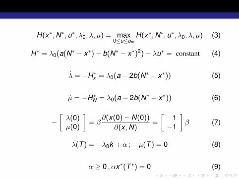
H(x∗, N∗, u∗, λ0, λ, µ) = max0≤u≤um
H(x∗, N∗, u∗, λ0, λ, µ) (3)
H∗ = λ0(a(N∗ − x∗)− b(N∗ − x∗)2)− λu∗ = constant (4)
λ = −H∗x = λ0(a− 2b(N∗ − x∗)) (5)
µ = −H∗N = λ0(a− 2b(N∗ − x∗)) (6)
−[
λ(0)µ(0)
]= β
∂(x(0)− N(0))
∂(x , N)=
[1
−1
]β (7)
λ(T ) = −λ0k + α ; µ(T ) = 0 (8)
α ≥ 0 , αx∗(T ∗) = 0 (9)
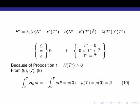
H∗ = λ0(a(N∗ − x∗(T ∗)− b(N∗ − x∗(T ∗))2)− λ(T ∗)u∗(T ∗)
≤=≥
0 if
T ∗ = 0
0 < T ∗ < TT ∗ = T
Because of Proposition 1 H(T ∗) ≥ 0From (6), (7), (8)∫ T
0HNdt = −
∫ T
0µdt = µ(0)− µ(T ) = µ(0) = β (10)
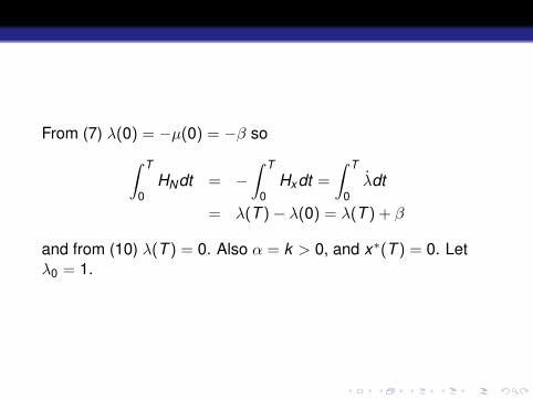
From (7) λ(0) = −µ(0) = −β so∫ T
0HNdt = −
∫ T
0Hxdt =
∫ T
0λdt
= λ(T )− λ(0) = λ(T ) + β
and from (10) λ(T ) = 0. Also α = k > 0, and x∗(T ) = 0. Letλ0 = 1.
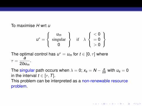
To maximise H wrt u
u∗ =
um
singular0
if λ
< 0= 0> 0
The optimal control has u∗ = um for t ∈ [0, τ ] where
τ =a
2bum.
The singular path occurs when λ = 0; xs = N − a2b with us = 0
in the interval t ∈ [τ, T ].This problem can be interpreted as a non-renewable resourceproblem.
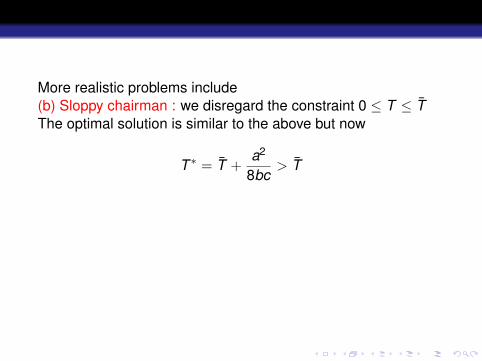
More realistic problems include(b) Sloppy chairman : we disregard the constraint 0 ≤ T ≤ TThe optimal solution is similar to the above but now
T ∗ = T +a2
8bc> T
(c) Forgetful audience : y = u − δy δ > 0δ may be regarded as the number of slides still kept in memoryat t by an average member of the audience.Similar result but now us > 0 (a more realistic result).(d) Stochastic chairman and presenterProbabilistic parameters.
More realistic problems include(b) Sloppy chairman : we disregard the constraint 0 ≤ T ≤ TThe optimal solution is similar to the above but now
T ∗ = T +a2
8bc> T
(c) Forgetful audience : y = u − δy δ > 0δ may be regarded as the number of slides still kept in memoryat t by an average member of the audience.Similar result but now us > 0 (a more realistic result).
(d) Stochastic chairman and presenterProbabilistic parameters.
More realistic problems include(b) Sloppy chairman : we disregard the constraint 0 ≤ T ≤ TThe optimal solution is similar to the above but now
T ∗ = T +a2
8bc> T
(c) Forgetful audience : y = u − δy δ > 0δ may be regarded as the number of slides still kept in memoryat t by an average member of the audience.Similar result but now us > 0 (a more realistic result).(d) Stochastic chairman and presenterProbabilistic parameters.

THANK YOU FOR YOUR PATIENT ATTENTION