Optimal Control Framework for a Centralized

Approach to Separation Management

Leif Walter1 and Ekaterina Kostina2

Philipps-University, 35037 Marburg, Germany

Matthias Poppe3

DFS Deutsche Flugsicherung GmbH, 63225 Langen, Germany

One key element of future Air Traffic Management concepts are automation tools that

help to separate aircraft from one another in a tactical environment. This paper is

devoted to capabilities of a centralized approach to separation or conflict manage-

ment, based on optimal control and its applications. We present an optimal control

framework that generates conflict-free trajectories for all aircraft within a regarded

airspace. The optimization process is based on the direct solution method for optimal

control problems and uses multiple shooting discretization with an SQP method to

solve the resulting nonlinear problem. Numerical computations are performed with

the MUSCOD-II software (IWR, University of Heidelberg). The principle advantage

of a centralized approach is that the optimal control framework consider complete in-

formation of the traffic situation in an airspace volume, thus it generates solutions that

incorporate information of all airspace users simultaneously. This prevents solutions

that could otherwise yield even more severe situations later in time. As an optimality

measure we use a performance index that aims to assess the deviation from a nominal

flight trajectory as filed by the user. Numerical experiments show that compared to

human solutions, the method proposed in this paper yields a significant decrease of

delay and flight track excess, as well as fuel savings of approximately 5%.

1 Optimization Workgroup, Faculty of Mathematics and Computer Science2 Head of Optimization Workgroup, Faculty of Mathematics and Computer Science3 Research & Development Department

1

I. Introduction

With the increase in demand and capacity, Air Traffic Management (ATM) will face further

challenges to keep delay considerably low while increasing safety standards at a cheaper cost. When

addressing these challenges imposed by future ATM programs (SESAR, NextGen), controllers will

need sophisticated decision support tools to deal with upcoming traffic flows in an efficient way.

As it was pointed out in the Performance Review Report 2010, [12], 5 % of all flights in Europe

are held on the ground to manage en-route congestion, resulting in more than 50 % of all delay

minutes within the system.

In the future, air navigation service providers (ANSPs) will need to deliver more capacity,

in a cheaper, safer, and environmental-friendlier way. This goal will not be achieved without the aid

of sophisticated and automated tools that will assist the human air traffic controller (ATCO). One

of the air traffic management fields that can contribute to provide to future capacity is separation

management. In the context of this paper, separation management is the task of separating aircraft

in an allocated airspace volume as efficiently as possible.

The aim of this paper is to present the application of optimal control theory in a central-

ized approach to separation management, where we use information of the current traffic situation

in a sector to derive an optimal control problem. The solution of this control problem consecutively

provide conflict-free trajectories for all users within the regarded airspace. Solutions are obtained

by using a direct method that is composed of multiple shooting discretization and a sequential

quadratic programming (SQP) method to solve the resulting nonlinear optimization problem.

This approach shows very promising results when applied to centralized separation manage-

ment. Numerical results are validated using real-time simulations performed at the Deutsche

Flugsicherung GmbH (DFS) research & development department. These trials demonstrate that

2

the optimal control framework proposed by the authors is able to deliver conflict solutions that

yield shorter track lengths, hence leading to a fuel saving of approximately up to 5%.

The paper is organized as follows. In Section II, we derive an optimal control problem by

using information on the current traffic situation and sketch the principles of the numerical method

used to solve the resulting optimal control problem. Numerical experiments using two scenarios

are discussed in Section III. Discussion and evaluation of the results are presented in Section IV.

II. Optimal Control Problem for Separation Management

In general, optimal control is applied to obtain control trajectories that will drive a dynamic

system from its initial state to its final state in an optimal way. Common applications include

processes in chemical industry, aerospace engineering or vehicle control. While optimization

methods are generally often used to engage challenges in ATM, as in [13], [7], [1], and [10], the

application of optimal control to separation management is still not a common approach. To our

knowledge, this paper is the first trial to formulate and to solve separation management problems

as optimal control problems.

In this Section, we first derive a generic problem formulation that can be used to formulate a control

problem for any traffic situation. The system dynamics (i.e. its propagator) is given by the aircraft

motions through airspace. Control inputs are the aircraft’s velocity and its bank angle. Terminal

conditions for initial and final states are determined by the aircraft’s entry point and its desired

destination. Separation minima are naturally formulated as path conditions, control constraints

incorporate information about individual aircraft capabilities. As we will see later, a suitable

formulation of the objective function is less straightforward than the formulation of the previous

items. In this approach, we want to minimize the total impact on the aircraft, so that an optimal

conflict resolution will be done with as less effort as necessary. The aim of the optimization is to

obtain control trajectories for all aircrafts’ velocity and bank angle. These control trajectories will

then ultimately result in optimal flight trajectories for each aircraft. Note that in this approach,

trajectories are optimized from a holistic, i.e. centralized, point of view.

3

A. Optimal Control Problem

The system of ordinary differential equations for the numerical examples that are studied in

Section III is chosen to represent the BADA (Base of Aircraft Data, [6]) model that is used within

the AFS (Advanced Function Simulator by DFS) real-time simulations. Since we only inspect 2-

dimensional en-route scenarios without level changes, the dynamic model is simplified to:

θi(t) =g

Vi(t)tan(µi(t)),

xi(t) = Vi(t) cos(θi(t)), (1)

yi(t) = Vi(t) sin(θi(t)), t ∈ [0, pi]

for each aircraft i = 1, 2, . . . ,m, where m is the total number of aircrafts. Here θi(t) is the aircraft

heading, Vi(t) is the true airspeed, µi(t) is the bank angle, xi(t) is the lateral and yi(t) is the

longitudinal positions. Control functions are the aircraft velocity and its bank angle, which means

ui0(t) := µi(t) and ui

1(t) := Vi(t). Each aircraft i spents time pi in the regarded airspace. Since

these times may be different for different aircrafts we apply time transormation of the time intervals

[t0, pi] into a fixed time interval [0, 1], include free end times pi as additional parameters into the

model and reformulate (1) as

θi(t) = pi g

Vi(t)tan(µi(t)),

xi(t) = piVi(t) cos(θi(t)),

yi(t) = piVi(t) sin(θi(t)), t ∈ [0, 1].

With the notations

u(t) =(u1

0(t), . . . , um0 (t), u1

1(t), . . . , um1 (t)

)T ∈ R2m,

ω(t) = (θ1(t), x1(t), y1(t), . . . , θm(t), xm(t), ym(t))T ∈ R3m,

p =(p1, . . . , pm

)T ∈ Rm,

f(ω(t), u(t), p) =(p1 g

V1(t)tan(µ1(t)), p1V1(t) cos(θ1(t)), p1V1(t) sin(θ1(t)), . . . ,

pm g

Vm(t)tan(µm(t)), pmVm(t) cos(θm(t)), pmVm(t) sin(θm(t))

)T

4

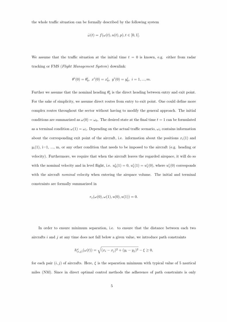
the whole traffic situation can be formally described by the following system

ω(t) = f(ω(t), u(t), p), t ∈ [0, 1].

We assume that the traffic situation at the initial time t = 0 is known, e.g. either from radar

tracking or FMS (Flight Management System) downlink:

θi(0) = θi0, x

i(0) = xi0, y

i(0) = yi0, i = 1, ...,m.

Further we assume that the nominal heading θi0 is the direct heading between entry and exit point.

For the sake of simplicity, we assume direct routes from entry to exit point. One could define more

complex routes throughout the sector without having to modify the general approach. The initial

conditions are summarized as ω(0) = ω0. The desired state at the final time t = 1 can be formulated

as a terminal condition ω(1) = ω1. Depending on the actual traffic scenario, ω1 contains information

about the corresponding exit point of the aircraft, i.e. information about the positions xi(1) and

yi(1), i=1, ..., m, or any other condition that needs to be imposed to the aircraft (e.g. heading or

velocity). Furthermore, we require that when the aircraft leaves the regarded airspace, it will do so

with the nominal velocity and in level flight, i.e. ui0(1) = 0, ui

1(1) = ui1(0), where ui

1(0) corresponds

with the aircraft nominal velocity when entering the airspace volume. The initial and terminal

constraints are formally summarized in

re(ω(0), ω(1), u(0), u(1)) = 0.

In order to ensure minimum separation, i.e. to ensure that the distance between each two

aircrafts i and j at any time does not fall below a given value, we introduce path constraints

hω(i,j)(ω(t)) =

√(xi − xj)2 + (yi − yj)2 − ξ ≥ 0,

for each pair (i, j) of aircrafts. Here, ξ is the separation minimum with typical value of 5 nautical

miles (NM). Since in direct optimal control methods the adherence of path constraints is only

5

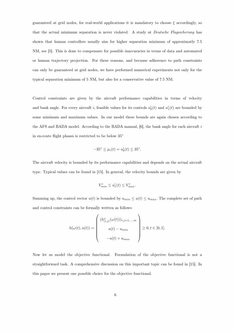
guaranteed at grid nodes, for real-world applications it is mandatory to choose ξ accordingly, so

that the actual minimum separation is never violated. A study at Deutsche Flugsicherung has

shown that human controllers usually aim for higher separation minimum of approximatly 7.5

NM, see [5]. This is done to compensate for possible inaccuracies in terms of data and automated

or human trajectory projection. For these reasons, and because adherence to path constraints

can only be guaranteed at grid nodes, we have performed numerical experiments not only for the

typical separation minimum of 5 NM, but also for a conservative value of 7.5 NM.

Control constraints are given by the aircraft performance capabilities in terms of velocity

and bank angle. For every aircraft i, feasible values for its controls ui0(t) and ui

1(t) are bounded by

some minimum and maximum values. In our model these bounds are again chosen according to

the AFS and BADA model. According to the BADA manual, [6], the bank angle for each aircraft i

in en-route flight phases is restricted to be below 35

−35 ≤ µi(t) = ui0(t) ≤ 35.

The aircraft velocity is bounded by its performance capabilities and depends on the actual aircraft

type. Typical values can be found in [15]. In general, the velocity bounds are given by

V imin ≤ ui

1(t) ≤ V imax.

Summing up, the control vector u(t) is bounded by umin ≤ u(t) ≤ umax. The complete set of path

and control constraints can be formally written as follows:

h(ω(t), u(t)) =

(hω

(i,j)(ω(t)))i,j=1,...,m

u(t)− umin

−u(t) + umax

≥ 0, t ∈ [0, 1].

Now let us model the objective functional. Formulation of the objective functional is not a

straightforward task. A comprehensive discussion on this important topic can be found in [15]. In

this paper we present one possible choice for the objective functional.

6

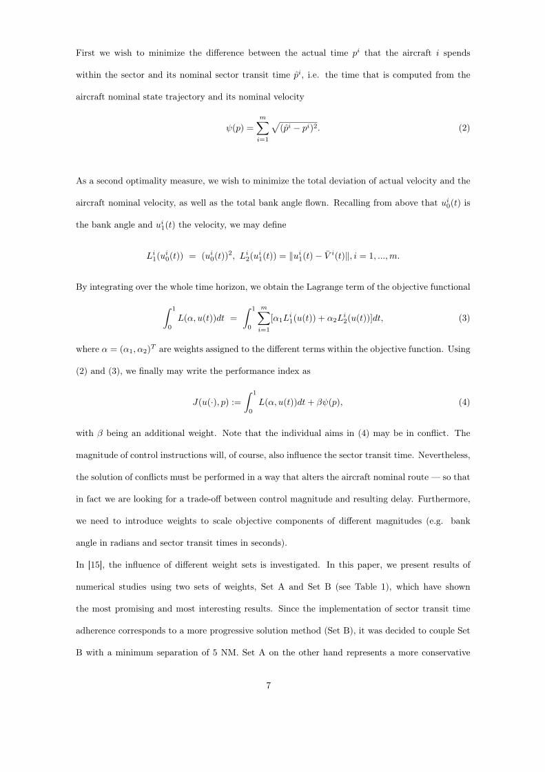
First we wish to minimize the difference between the actual time pi that the aircraft i spends

within the sector and its nominal sector transit time pi, i.e. the time that is computed from the

aircraft nominal state trajectory and its nominal velocity

ψ(p) =m∑

i=1

√(pi − pi)2. (2)

As a second optimality measure, we wish to minimize the total deviation of actual velocity and the

aircraft nominal velocity, as well as the total bank angle flown. Recalling from above that ui0(t) is

the bank angle and ui1(t) the velocity, we may define

Li1(ui

0(t)) = (ui0(t))2, Li

2(ui1(t)) = ‖ui

1(t)− V i(t)‖, i = 1, ...,m.

By integrating over the whole time horizon, we obtain the Lagrange term of the objective functional

∫ 1

0

L(α, u(t))dt =∫ 1

0

m∑i=1

[α1Li1(u(t)) + α2L

i2(u(t))]dt, (3)

where α = (α1, α2)T are weights assigned to the different terms within the objective function. Using

(2) and (3), we finally may write the performance index as

J(u(·), p) :=∫ 1

0

L(α, u(t))dt+ βψ(p), (4)

with β being an additional weight. Note that the individual aims in (4) may be in conflict. The

magnitude of control instructions will, of course, also influence the sector transit time. Nevertheless,

the solution of conflicts must be performed in a way that alters the aircraft nominal route — so that

in fact we are looking for a trade-off between control magnitude and resulting delay. Furthermore,

we need to introduce weights to scale objective components of different magnitudes (e.g. bank

angle in radians and sector transit times in seconds).

In [15], the influence of different weight sets is investigated. In this paper, we present results of

numerical studies using two sets of weights, Set A and Set B (see Table 1), which have shown

the most promising and most interesting results. Since the implementation of sector transit time

adherence corresponds to a more progressive solution method (Set B), it was decided to couple Set

B with a minimum separation of 5 NM. Set A on the other hand represents a more conservative

7

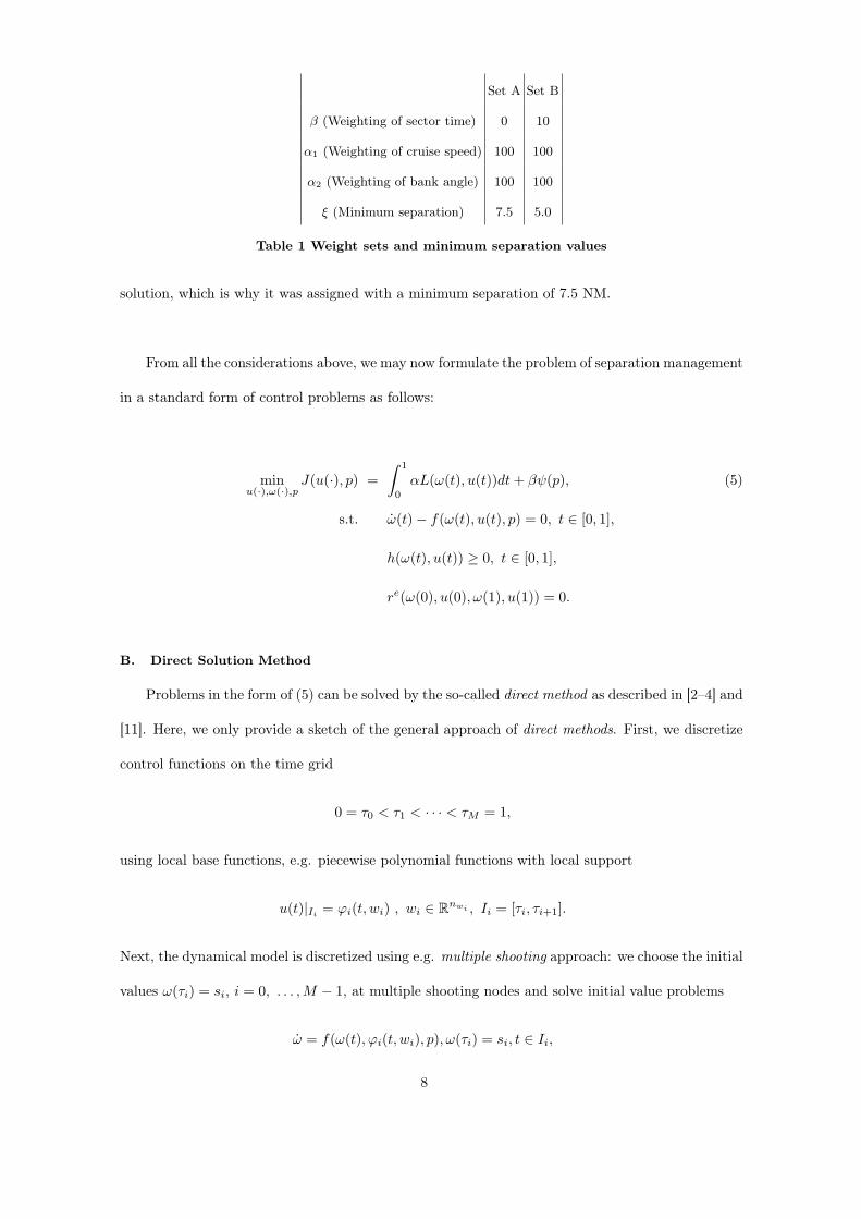
Set A Set B

β (Weighting of sector time) 0 10

α1 (Weighting of cruise speed) 100 100

α2 (Weighting of bank angle) 100 100

ξ (Minimum separation) 7.5 5.0

Table 1 Weight sets and minimum separation values

solution, which is why it was assigned with a minimum separation of 7.5 NM.

From all the considerations above, we may now formulate the problem of separation management

in a standard form of control problems as follows:

minu(·),ω(·),p

J(u(·), p) =∫ 1

0

αL(ω(t), u(t))dt+ βψ(p), (5)

s.t. ω(t)− f(ω(t), u(t), p) = 0, t ∈ [0, 1],

h(ω(t), u(t)) ≥ 0, t ∈ [0, 1],

re(ω(0), u(0), ω(1), u(1)) = 0.

B. Direct Solution Method

Problems in the form of (5) can be solved by the so-called direct method as described in [2–4] and

[11]. Here, we only provide a sketch of the general approach of direct methods. First, we discretize

control functions on the time grid

0 = τ0 < τ1 < · · · < τM = 1,

using local base functions, e.g. piecewise polynomial functions with local support

u(t)|Ii = ϕi(t, wi) , wi ∈ Rnwi , Ii = [τi, τi+1].

Next, the dynamical model is discretized using e.g. multiple shooting approach: we choose the initial

values ω(τi) = si, i = 0, . . . ,M − 1, at multiple shooting nodes and solve initial value problems

ω = f(ω(t), ϕi(t, wi), p), ω(τi) = si, t ∈ Ii,

8

resulting in the trajectories ω(t; si, wi, p), t ∈ Ii, i = 0, ...,M − 1. The continuity of the optimal

trajectory is ensured by the following constraints

ω(τi+1; si, wi, p)− si+1 = 0 , i = 0, . . . ,M − 1,

which are included into optimization problem. Furthermore, we discretize the cost functional and

path, as well as control constraints accordingly.

As a result, the optimal control problem is transformed as a finite-dimensional optimization

problem that can be written in the form

minxf(x), s.t. g(x) = 0, c(x) ≥ 0,

where the variables x include s0, w0, . . . , sM−1, wM−1, sM , p. These finite-dimensional optimization

problems are typically adressed by descent algorithms as described in [9].

Here, we chose to solve the problem using the sequential quadratic programming method (SQP)

according to which the new iteration is computed by

xk+1 = xk + tk∆xk,

where the increment ∆xk solves the quadratic problem

min∆x∈Ωk

12

∆xTHk∆x+∇f(xk)T ∆x

g(xk) +∇g(xk)T ∆x = 0, c(xk) +∇c(xk)T ∆x ≥ 0,

where Hk approximates the Hessian of the Langrange function at the current iteration. More

details on the SQP method can be found in [9]. The SQP algorithm itself can be adapted by

choosing different strategies for approximating the Hessian of the Lagrangian, and by choosing a

globalization technique. In the numerical experiments of this paper we have used the software

package MUSCOD-II, where the SQP module has been configured to use a BFGS update on the

Hessian approximation of the the Langrange function, as well as a VMCWD (Variable Metric

Constrained WatchDog) technique to determine the step length, see [14].

9

III. Numerical Experiments: Scenarios

In order to test the proposed approach to separation management six traffic scenarios have been

investigated in [15]. Due to lack of place we present the detailed results of two scenarios, namely

scenarios B and E, that proved to be the most interesting. In all scenarios we consider a synthetic

sector of 100 NM × 100 NM on a flight altitude of 35000 Ft, which is typical for en-route flight

phase. Each scenario involves four aircrafts thus having higher-order conflicts.

For each scenario, we compare the numerical solutions obtained by the optimal control procedure

with the solutions obtained by human Air Traffic Controllers (ATCO). The comparison is performed

in terms of delays, flight tracks and magnitude of clearances. For the sake of clarity, human ATCO

solutions are presented as average values. As mentioned above, we present two numerical solutions

for each scenario: a conservative solution (Cons), not considering a deviation in sector transit time

and using a separation minimum of 7.5 NM — and a more progressive solution (Pro), also aiming

for an exact match in sector transit time and using a separation minimum of 5 NM. The values of

the weights and setups for numerical solutions are presented in Table 1, Set A for a conservative

and Set B for a progressive solution.

A. Scenario B: Flight Level Rogue

In Scenario B, a slower aircraft (aircraft 4, Cessna C550) is flying ahead of aircraft 1 (B738)

— while both aircraft are heading for the eastern airspace border. Therefore, a solution must be

found that either slows down aircraft 1 significantly, or provides heading changes that enable an

overtaking maneuver. For description of Scenario B see Table 2.

No. Type Entry Exit

1 B737-800 (000, 050) (100, 050)

2 B737-800 (100, 050) (000, 050)

3 B737-800 (050, 000) (050, 100)

4 Cessna 550 (010, 050) (100, 050)

Table 2 Description of Scenario B

10

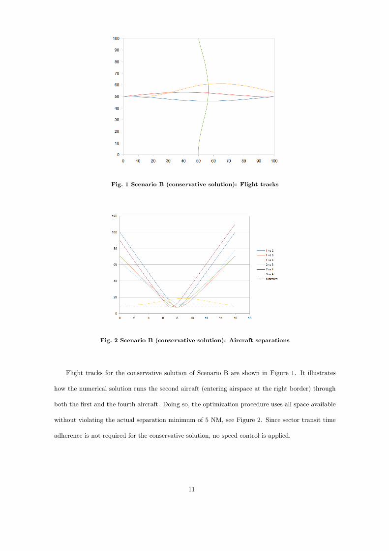
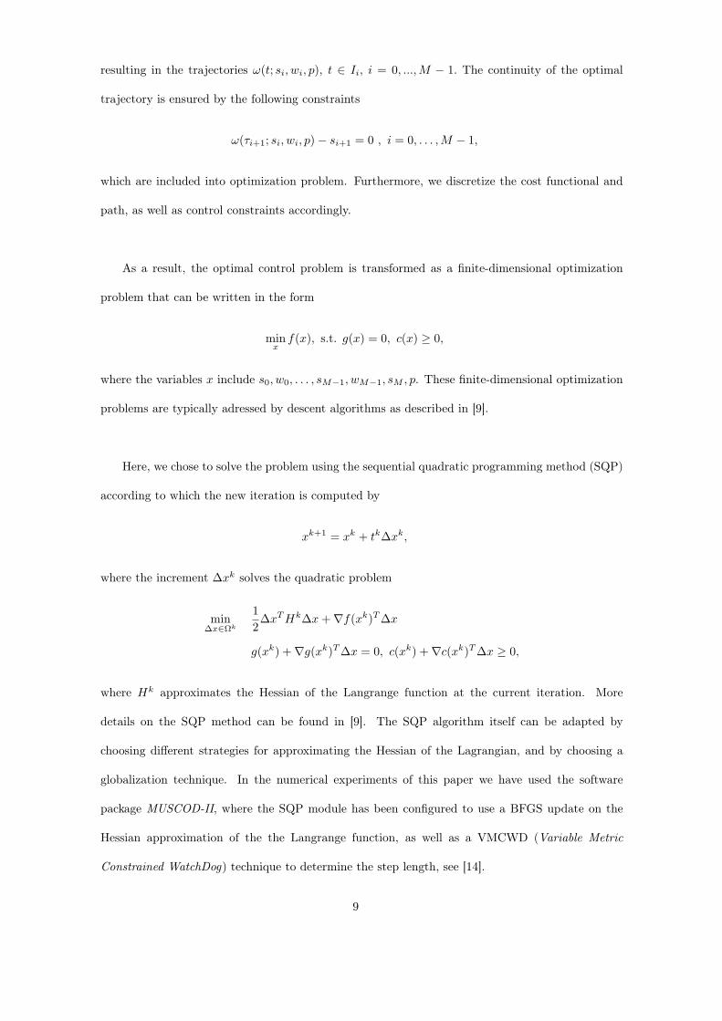
Fig. 1 Scenario B (conservative solution): Flight tracks

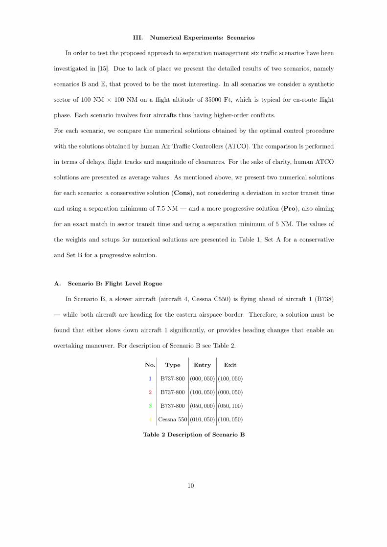
Fig. 2 Scenario B (conservative solution): Aircraft separations

Flight tracks for the conservative solution of Scenario B are shown in Figure 1. It illustrates

how the numerical solution runs the second aircaft (entering airspace at the right border) through

both the first and the fourth aircraft. Doing so, the optimization procedure uses all space available

without violating the actual separation minimum of 5 NM, see Figure 2. Since sector transit time

adherence is not required for the conservative solution, no speed control is applied.

11

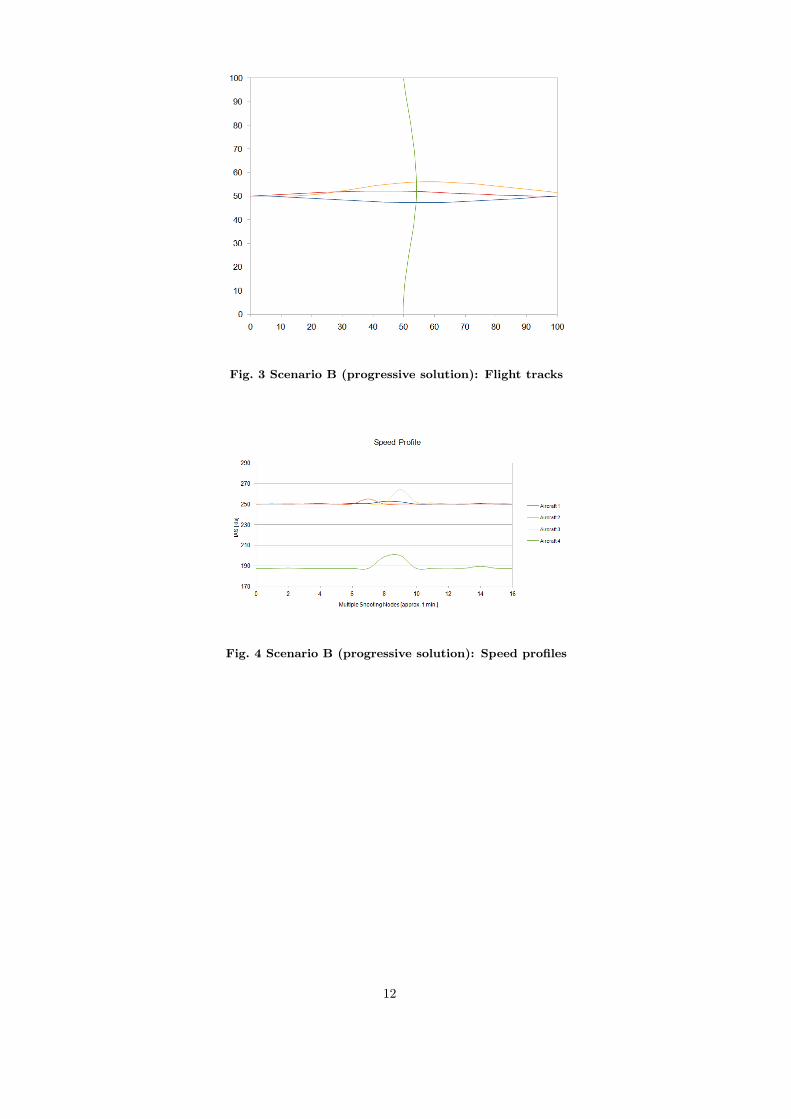
Fig. 3 Scenario B (progressive solution): Flight tracks

Fig. 4 Scenario B (progressive solution): Speed profiles

12

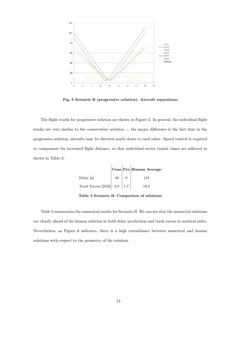
Fig. 5 Scenario B (progressive solution): Aircraft separations

The flight tracks for progressive solution are shown in Figure 3. In general, the individual flight

tracks are very similar to the conservative solution — the major difference is the fact that in the

progressive solution, aircrafts may be directed much closer to each other. Speed control is required

to compensate for increased flight distance, so that individual sector transit times are adhered as

shown in Table 3.

Cons Pro Human Average

Delay/[s] 49 0 119

Track Excess/[NM] 4.9 1.7 19.4

Table 3 Scenario B: Comparison of solutions

Table 3 summarizes the numerical results for Scenario B. We can see that the numerical solutions

are clearly ahead of the human solution in both delay production and track excess in nautical miles.

Nevertheless, as Figure 6 indicates, there is a high resemblance between numerical and human

solutions with respect to the geometry of the solution.

13

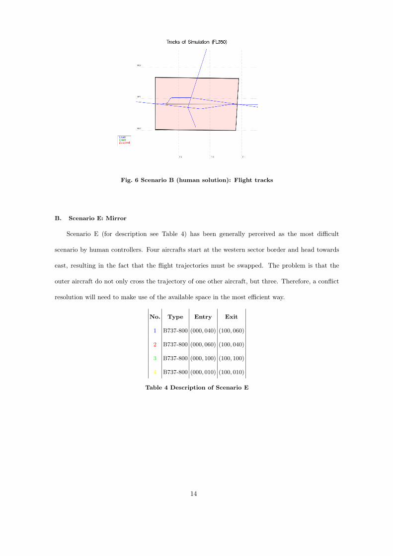
Fig. 6 Scenario B (human solution): Flight tracks

B. Scenario E: Mirror

Scenario E (for description see Table 4) has been generally perceived as the most difficult

scenario by human controllers. Four aircrafts start at the western sector border and head towards

east, resulting in the fact that the flight trajectories must be swapped. The problem is that the

outer aircraft do not only cross the trajectory of one other aircraft, but three. Therefore, a conflict

resolution will need to make use of the available space in the most efficient way.

No. Type Entry Exit

1 B737-800 (000, 040) (100, 060)

2 B737-800 (000, 060) (100, 040)

3 B737-800 (000, 100) (100, 100)

4 B737-800 (000, 010) (100, 010)

Table 4 Description of Scenario E

14

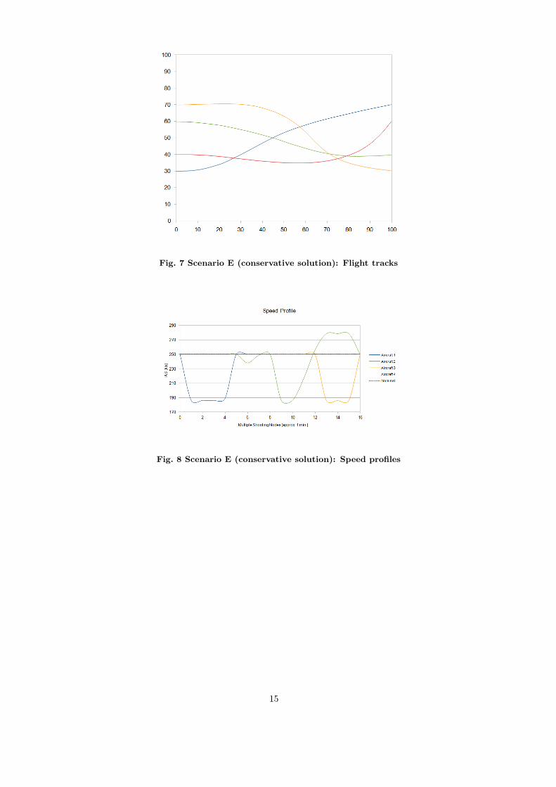
Fig. 7 Scenario E (conservative solution): Flight tracks

Fig. 8 Scenario E (conservative solution): Speed profiles

15

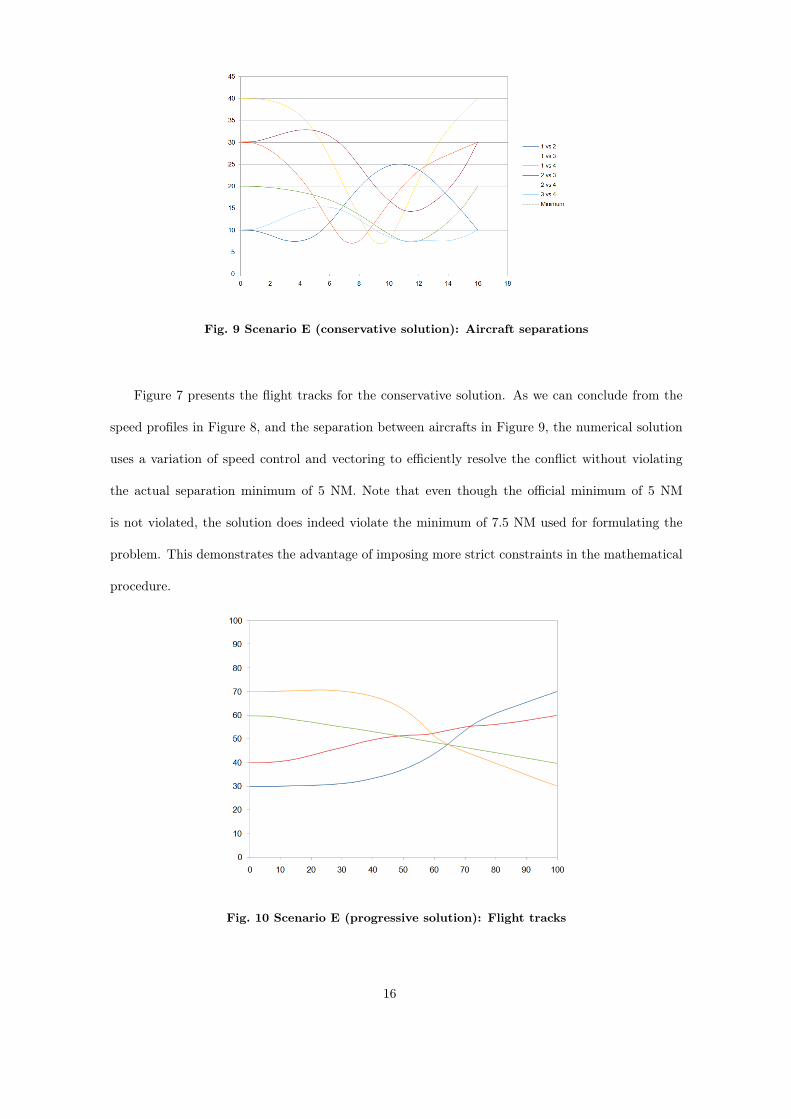
Fig. 9 Scenario E (conservative solution): Aircraft separations

Figure 7 presents the flight tracks for the conservative solution. As we can conclude from the

speed profiles in Figure 8, and the separation between aircrafts in Figure 9, the numerical solution

uses a variation of speed control and vectoring to efficiently resolve the conflict without violating

the actual separation minimum of 5 NM. Note that even though the official minimum of 5 NM

is not violated, the solution does indeed violate the minimum of 7.5 NM used for formulating the

problem. This demonstrates the advantage of imposing more strict constraints in the mathematical

procedure.

Fig. 10 Scenario E (progressive solution): Flight tracks

16

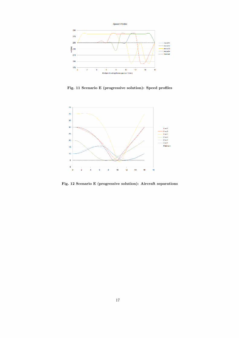
Fig. 11 Scenario E (progressive solution): Speed profiles

Fig. 12 Scenario E (progressive solution): Aircraft separations

17

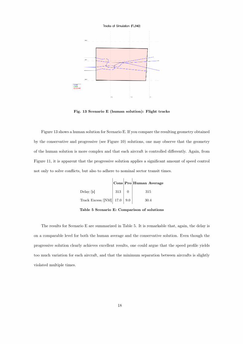
Fig. 13 Scenario E (human solution): Flight tracks

Figure 13 shows a human solution for Scenario E. If you compare the resulting geometry obtained

by the conservative and progressive (see Figure 10) solutions, one may observe that the geometry

of the human solution is more complex and that each aircraft is controlled differently. Again, from

Figure 11, it is apparent that the progressive solution applies a significant amount of speed control

not only to solve conflicts, but also to adhere to nominal sector transit times.

Cons Pro Human Average

Delay/[s] 313 0 315

Track Excess/[NM] 17.0 9.0 30.4

Table 5 Scenario E: Comparison of solutions

The results for Scenario E are summarized in Table 5. It is remarkable that, again, the delay is

on a comparable level for both the human average and the conservative solution. Even though the

progressive solution clearly achieves excellent results, one could argue that the speed profile yields

too much variation for each aircraft, and that the minimum separation between aircrafts is slightly

violated multiple times.

18

IV. Numerical Experiments: Evaluation and Discussion

As we have seen in the previous section, the results obtained by the proposed approach are

very promising. The fact that the numerical solutions yield much better results in terms of delay

and flight track excess shows the potential efficiency of the method. Similar results are obtained in

numerical experiments with other scenarios, the detailed description of which can be found in [15].

The results of the numerical experiments in all scenarios allow the following interpretations.

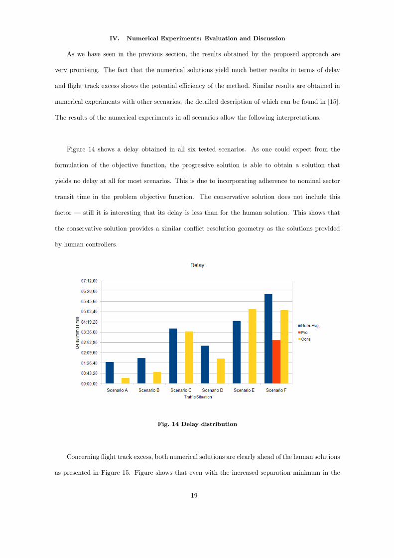
Figure 14 shows a delay obtained in all six tested scenarios. As one could expect from the

formulation of the objective function, the progressive solution is able to obtain a solution that

yields no delay at all for most scenarios. This is due to incorporating adherence to nominal sector

transit time in the problem objective function. The conservative solution does not include this

factor — still it is interesting that its delay is less than for the human solution. This shows that

the conservative solution provides a similar conflict resolution geometry as the solutions provided

by human controllers.

Fig. 14 Delay distribution

Concerning flight track excess, both numerical solutions are clearly ahead of the human solutions

as presented in Figure 15. Figure shows that even with the increased separation minimum in the

19

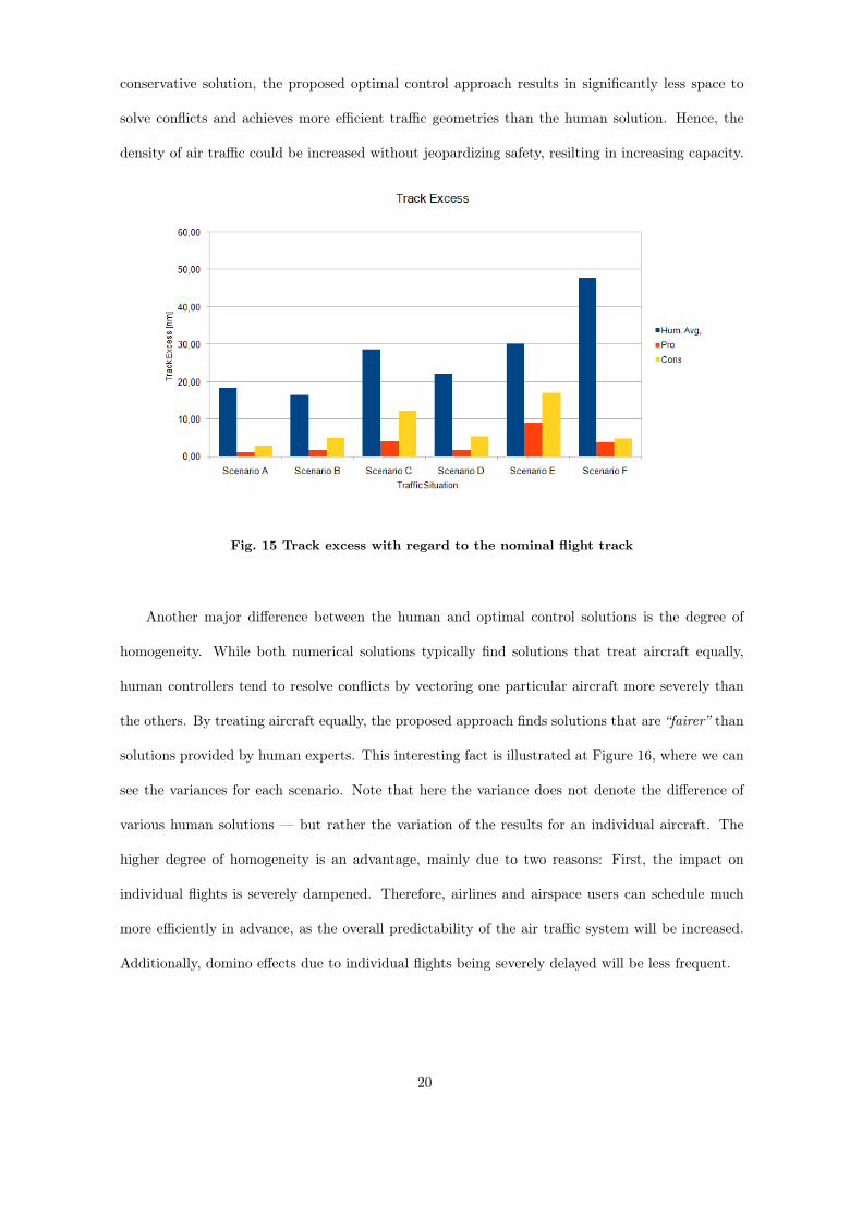
conservative solution, the proposed optimal control approach results in significantly less space to

solve conflicts and achieves more efficient traffic geometries than the human solution. Hence, the

density of air traffic could be increased without jeopardizing safety, resilting in increasing capacity.

Fig. 15 Track excess with regard to the nominal flight track

Another major difference between the human and optimal control solutions is the degree of

homogeneity. While both numerical solutions typically find solutions that treat aircraft equally,

human controllers tend to resolve conflicts by vectoring one particular aircraft more severely than

the others. By treating aircraft equally, the proposed approach finds solutions that are “fairer” than

solutions provided by human experts. This interesting fact is illustrated at Figure 16, where we can

see the variances for each scenario. Note that here the variance does not denote the difference of

various human solutions — but rather the variation of the results for an individual aircraft. The

higher degree of homogeneity is an advantage, mainly due to two reasons: First, the impact on

individual flights is severely dampened. Therefore, airlines and airspace users can schedule much

more efficiently in advance, as the overall predictability of the air traffic system will be increased.

Additionally, domino effects due to individual flights being severely delayed will be less frequent.

20

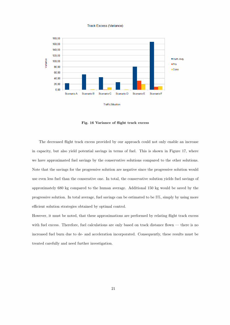
Fig. 16 Variance of flight track excess

The decreased flight track excess provided by our approach could not only enable an increase

in capacity, but also yield potential savings in terms of fuel. This is shown in Figure 17, where

we have approximated fuel savings by the conservative solutions compared to the other solutions.

Note that the savings for the progressive solution are negative since the progressive solution would

use even less fuel than the conserative one. In total, the conservative solution yields fuel savings of

approximately 680 kg compared to the human average. Additional 150 kg would be saved by the

progressive solution. In total average, fuel savings can be estimated to be 5%, simply by using more

efficient solution strategies obtained by optimal control.

However, it must be noted, that these approximations are performed by relating flight track excess

with fuel excess. Therefore, fuel calculations are only based on track distance flown — there is no

increased fuel burn due to de- and acceleration incorporated. Consequently, these results must be

treated carefully and need further investigation.

21

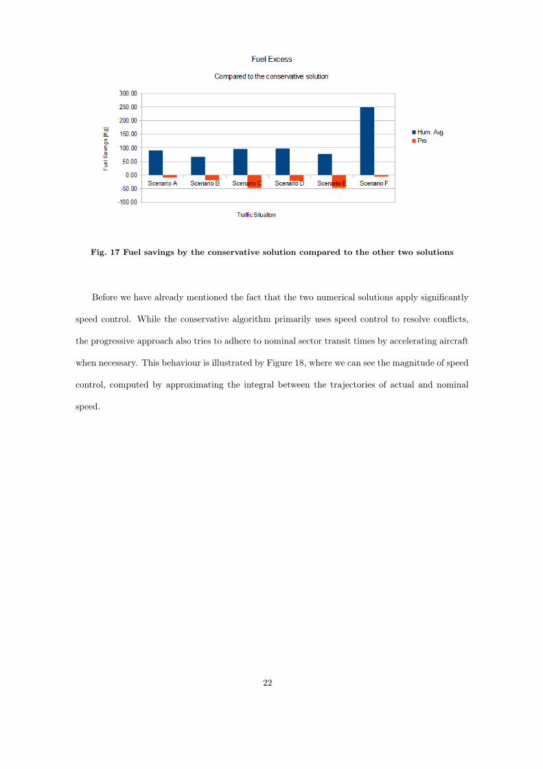
Fig. 17 Fuel savings by the conservative solution compared to the other two solutions

Before we have already mentioned the fact that the two numerical solutions apply significantly

speed control. While the conservative algorithm primarily uses speed control to resolve conflicts,

the progressive approach also tries to adhere to nominal sector transit times by accelerating aircraft

when necessary. This behaviour is illustrated by Figure 18, where we can see the magnitude of speed

control, computed by approximating the integral between the trajectories of actual and nominal

speed.

22

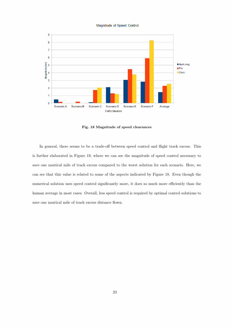
Fig. 18 Magnitude of speed clearances

In general, there seems to be a trade-off between speed control and flight track excess. This

is further elaborated in Figure 19, where we can see the magnitude of speed control necessary to

save one nautical mile of track excess compared to the worst solution for each scenario. Here, we

can see that this value is related to some of the aspects indicated by Figure 18. Even though the

numerical solution uses speed control significantly more, it does so much more efficiently than the

human average in most cases. Overall, less speed control is required by optimal control solutions to

save one nautical mile of track excess distance flown.

23

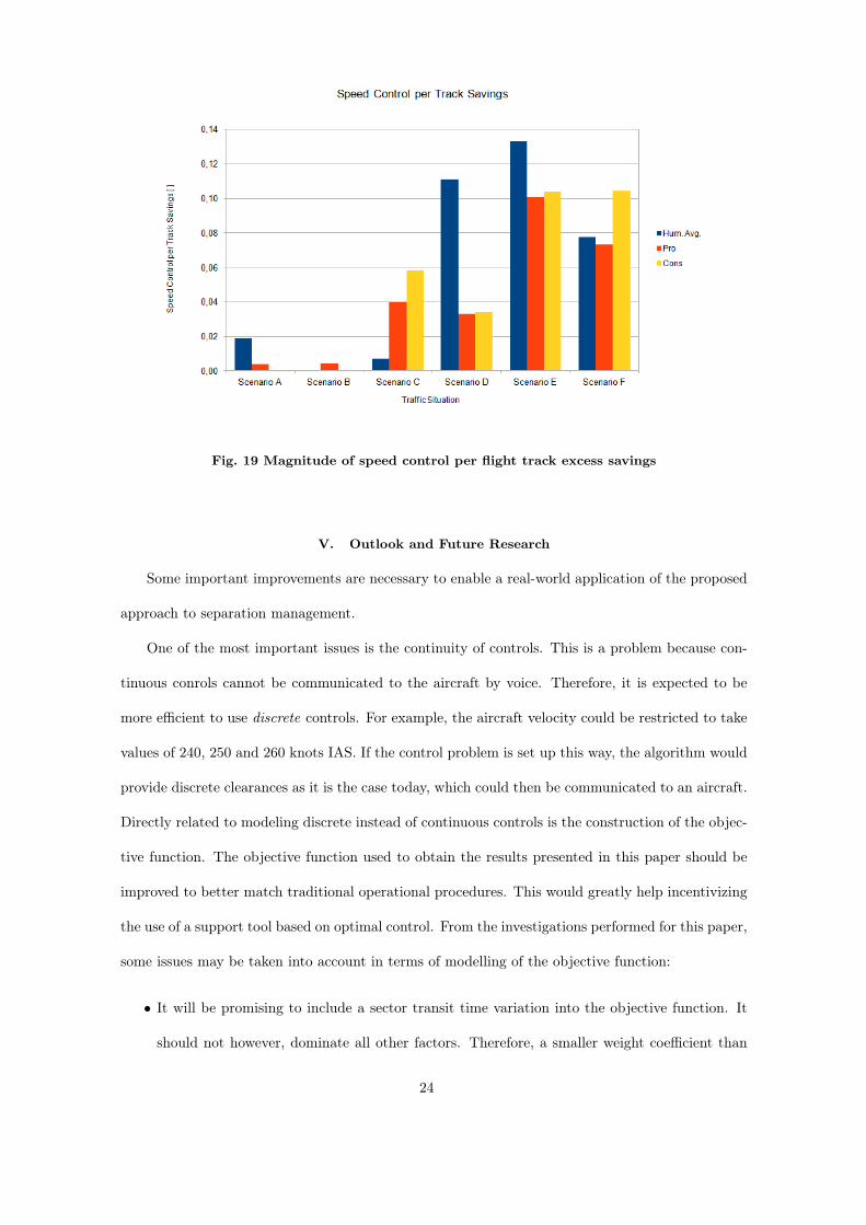
Fig. 19 Magnitude of speed control per flight track excess savings

V. Outlook and Future Research

Some important improvements are necessary to enable a real-world application of the proposed

approach to separation management.

One of the most important issues is the continuity of controls. This is a problem because con-

tinuous conrols cannot be communicated to the aircraft by voice. Therefore, it is expected to be

more efficient to use discrete controls. For example, the aircraft velocity could be restricted to take

values of 240, 250 and 260 knots IAS. If the control problem is set up this way, the algorithm would

provide discrete clearances as it is the case today, which could then be communicated to an aircraft.

Directly related to modeling discrete instead of continuous controls is the construction of the objec-

tive function. The objective function used to obtain the results presented in this paper should be

improved to better match traditional operational procedures. This would greatly help incentivizing

the use of a support tool based on optimal control. From the investigations performed for this paper,

some issues may be taken into account in terms of modelling of the objective function:

• It will be promising to include a sector transit time variation into the objective function. It

should not however, dominate all other factors. Therefore, a smaller weight coefficient than

24

used in the progressive solution seems reasonable.

• To prevent the algorithm to focus on speed control, the weight coefficient α2 for speed varia-

tions should be increased.

• Minimizing the total bank angle flown as done for this paper might not always be the best

solution. Instead, auxiliary variables should be included that compute the total variation

in flight track distance flown, so that this factor can be taken into account in the objective

function.

• More generally, since we need to optimize several sometimes conflicting objectives, numerical

studies from the point of view of multicriterial optimization would be helpfull for an appro-

priate choice of weight coefficients in the objective function.

For numerical solutions the path constraints may be violated between time discretization grid

nodes. Since the violation of the separation minimum is not allowed, one should use robustification

of the path constraints as discussed e.g. in [8].

Another important issue is repeated update of traffic situation. The constrained optimal control

problem (5) considered in this paper treats one particular traffic situation. In reality however,

air traffic is propagating in streams or flows of aircraft, where the situation in an actual airspace

will change continuously. While one aircraft will leave a particular airspace, others will enter

it. Therefore, it is reasonable to emphasize the installment of a control loop that will re-assess

the traffic situation at a constant rate, hence adapting the control problem (5) and its con-

straints. By using a loop structure of continuously connected optimal control problems we may

obtain a feedback law that will yield a control strategy able to process possible perturbations

and data inaccuracies. In case the basic structure of the problem remains the same (i.e. no air-

craft have entered or left the sector), this framework would lead to a NMPC implementation, see [3].

Last but not least, an interesting enhancenment of the model are the implementation of

three-dimensional dynamics as well as weather and wind effects.

25

VI. Conclusions

In this paper, we have presented a framework for resolving air traffic conflict situations by

providing conflict-free and optimal trajectories for all airspace users. This framework is based on

optimal control theory, which is a new approach to a centralized separation management. We

have presented details of numerical experiments for two different traffic scenarios, as well as the

discussion of the numerical experiments for the set of six scenarios presented in details in [15].

These scenarios have been designed to represent worst-case traffic situations, incorporating conflicts

between multiple aircrafts. The numerical results obtained by solution of optimal control problems

have been then compared to real-time simulations performed by human controllers who have solved

the same traffic scenarios.

Results from these experiments have clearly shown that, compared to the human average, the

optimal control solutions have achieved better results. The delays are considerably lower, partic-

ularly for the progressive solution strategy. At the same time, the numerical solutions cause less

flight track excess, i.e. the actual distance flown by the aircraft is reduced. The savings in terms of

track distance flown are significant: In total, the human average has a track excess of 27 NM, while

the automated solution yields in average 3.6 NM for the progressive solution, and 7.8 NM for the

conservative solution. These savings are primarily due to two factors: First of all, the numerical

solutions use the available airspace more efficiently. As we have seen, the optimal control process

controls aircraft such that aircraft are separated very closely to the separation minimum. While

human controllers typically aim for a separation of 7.5 NM or more (as it has been the case during

the simulations), the optimal control procedure is able to aim for a lower value while still ensuring

the official minimum separation of 5 NM. As a second reason, it can be seen that the numerical

solutions use speed control to a greater extent and more efficiently than the human average. More-

over, it is also shown that the optimal control procedure uses speed control more efficiently. Another

potential of optimal control in separation management is yielding significant fuel savings of up to

5% with no workload for the human controller in terms of actual conflict resolution.

Results of numerical experiments also indicate that the approach must be further adapted to enable

26

a possible application in the real-world as a human controller assistance tool. Further research for

the application of optimal control in air traffic control is of great importance.

Acknowledgments

The authors would like to thank Deutsche Flugsicherung GmbH (DFS) for the collaboration in

this project. In particular, this project has been supported by the DFS R&D department as well

as the department for ATM Operations & Strategy. The authors are also thankful to Prof. Dr.

Dr. h.c. Hans Georg Bock (IWR, University of Heidelberg) for support in using software package

MUSCOD-II.

References

[1] F. Bellomi, R. Bonato, V. Nanni, and A. Tedeschi. Satisficing game theory for conflict resolution and

traffic optimization. Air Traffic Control Quarterly, 16(3):211–233, 2008.

[2] H.G. Bock and K.J. Plitt. A multiple shooting algorithm for direct solution of optimal control problems.

In Proceedings of the IFAC 9th World Congress, pages 242–247, July 2-6 1984.

[3] M. Diehl. Real-Time Optimization for Large Scale Nonlinear Processes. PhD thesis, Ruprecht-Karls-

Universität Heidelberg, 2001.

[4] P.J. Enright and B.A. Conway. Discrete approximations to optimal trajectories using direct transcrip-

tion and nonlinear programming. AIAA Paper 90-2963-CP, 1990.

[5] Deutsche Flugsicherung GmbH Forschung & Entwicklung. Staffelungsverhalten ACC Frankfurt. Jour-

Fixe, June 2001.

[6] Eurocontrol Experimental Centre. User Manual for the Base of Aircraft Data (BADA), 3.7 edition,

2009.

[7] A. Lecchini, W. Glover, J. Lygeros, and J. Maciejowski. Model predictive control formulation of conflict

resolution task. Hybridge Work Package 5: Control of Uncertain Hybrid Systems, 2004.

[8] M.Diehl, E.A.Kostina, and H.G.Bock. An approximation technique for robust nonlinear optimization.

Mathematical Programming, 107:213–230, 2006.

[9] J. Nocedal and S.J. Wright. Numerical Optimization. Springer Series in Operations Research. Springer,

2 edition, 2006.

[10] J. Omer and T. Chaboud. Tactical and post-tactical air traffic control methods. 9th Innovative Research

Workshop & Exhibition, 2010.

27

[11] P. Krämer-Eis. Ein Mehrzielverfahren zur Numerischen Berechnung Optimaler Feedback-Steuerungen

bei Beschränkten Nichtlinearen Steuerungsproblemen. PhD thesis, Universität Bonn, 1985.

[12] Performance Review Commission. Performance review report 2010. 2011.

[13] Clement Peyronne, Daniel Delahaye, Marcel Mongeau, and Laurent Lapasset. Optimizing b-splines

using genetic algorithms applied to air-traffic conflict resolution. In IJCCI (ICEC)’10, pages 213–218,

2010.

[14] M.J.D. Powell. Vmcwd: a fortran subroutine for constrained optimization. Newsletter ACM SIGMAP

Bulletin, (32), 1983.

[15] L. Walter. Direct optimal control methods for a centralized approach to separation management.

Diploma Thesis, January 2012.

28