Optimal control in an inventory management problem

Bulletin of the JSME

Journal of Advanced Mechanical Design, Systems, and ManufacturingVol.13, No.1, 2019

Paper No.17-00631© 2019 The Japan Society of Mechanical Engineers[DOI: 10.1299/jamdsm.2019jamdsm0008]

Optimal control in an inventory management problemconsidering replenishment lead time based upon a

non-diffusive stochastic differential equationHiroaki T.-KANEKIYO∗ and Shinjiro AGATA∗∗

∗ Dept. of Civil, Environmental and Systems Engineering, Kansai University3-3-35 Yamate-cho, Suita-city, Osaka, 564-8680, Japan

E-mail: [email protected]∗∗ Agata Iron Works Co., Ltd.

1-1-3 Sawakihama, Mito-cho, Toyokawa-city, Aichi, 441-0304, Japan

AbstractAn inventory management problem is theoretically discussed for a factory having effects of lead times in replen-ishing the inventory, where it stocks materials used for its products. It is assumed that the factory can dynamicallycontrol the size of ordering materials. By applying the stochastic control theory, the optimal control of the orderingsize is derived, in which the expected total cost up to an expiration time is minimized. First, a new stochastic modelis constructed for describing an inventory fluctuation of the factory by the use of a non-diffusive stochastic differ-ential equation, where an analytic time is introduced so that the inventory process can be a Markov process eventhough it is affected by lead times. Next, an optimal control is formulated by introducing an evaluation functionquantifying total costs. Based upon them, the Hamilton-Jacobi-Bellman (HJB) equation is derived, whose solutiongives the optimal control. Finally, the optimal control is quantitatively examined through numerical solutions ofthe HJB equation. Numerical results indicate that if time up to an expiration time is short then the optimal controlis affected by it, otherwise, the optimal control does not depend on it.

1. Introduction

For factories and retail stores, it is undoubtedly important to keep an adequate amount of inventories, which aresupposed to be materials for products or products themselves. They generally have to spend higher cost holding too largeamount of inventory, whereas they might lose opportunities for selling their products owing to shortages of the inventory.We should always perform the best control of the inventory level.

In the mathematical theory of inventory management, we can roughly classify continuous-time models describingtemporal variation of the inventory level into two types. One is suitable for expressing the inventory level of a massproduction factory(Rempała 2005), which manufactures a large amount of products whereas it receives a large ordersfrom customers such as orders from wholesale stores. Thus, the increase of its inventory level can be treated as continuousvariation whereas the decrease can be treated as discontinuous variation with discrete jumps. The other type is used forrepresenting that of a retail store (Feng and Rao 2007), which receives small orders from many customers, such as ordersfrom consumers whereas it makes a large order for products to suppliers at some intervals. Thus, the decrease of itsinventory level can be treated as continuous variation whereas the increase can be treated as discontinuous variation withdiscrete jumps.

However, there are some factories having intermediate characteristic between these two types (Chen, Feng and Ou2006). One example is a factory which manufactures steel products for construction of buildings. The outline of work inthe factory is as follows;

1

Received: 24 November 2017; Revised: 9 September 2018; Accepted: 10 January 2019

Keywords : Inventory, Optimal control, Lead time, Stochastic differential equation, Stochastic control

2© 2019 The Japan Society of Mechanical Engineers[DOI: 10.1299/jamdsm.2019jamdsm0008]

Kanekiyo and Agata, Journal of Advanced Mechanical Design, Systems, and Manufacturing, Vol.13, No.1 (2019)

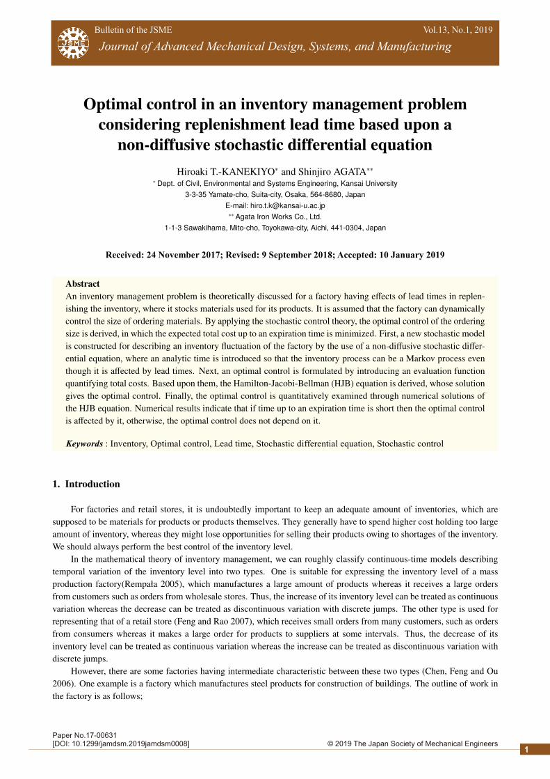
(i)The factory occasionally receives orders for steel products from several customers. The factory ordinarily manufac-tures some components for ordered products by cutting steel plates stocked in its warehouse, which is called shearingprocedure. Then it assembles the components into the ordered products.

(ii)When stocked plates get fewer, the factory orders some steel plates to a steel plate supplier. The factory has to waituntil it gets the ordered plates, which is the so-called lead time.

(iii)When the current inventory is under the amount of steel plates necessary for an order from a customer, the factoryimmediately compensates the shortage of components by ordering them to external components suppliers.

Such an intermediate characteristic expressing a diagram of works is schematically illustrated in Fig.1.

materialsupplier

factory

warehous

materials

components

products

customers

external

components

suppliers

ordinary order customer order

manufacturing

order

assembling

urgent

Fig. 1 Schematic diagram of the system of a factory and its related factors.

Taking such characteristics of the factory into consideration, we construct a stochastic model describing the inventoryfluctuation so that it is also applicable to several factories whose inventory fluctuations are similar to the intermediatecharacteristic as illustrated in Fig.1. If we rigorously formulate the inventory fluctuation reflecting characteristics above,we have a serious problem when we apply the stochastic control theory, which is often used in the inventory managementproblem to obtain the optimal control, i.e., the stochastic process describing the inventory level is not a Markov processbecause of the above-mentioned lead time. In order to remove the problem, we newly propose an improved model of theinventory fluctuation by introducing a new time variable, in which a stochastic differential equation driven by a compoundPoisson process is applied (Øksendal and Sulem 2007, Applebaum 2009 and Kanekiyo 2014). Based upon the improvedmodel, we introduce an evaluation function, which consists of two kinds of costs, to formulate the optimal control. Oneis the cost for holding the inventory and the other is the cost for ordering to external components suppliers.

The main purpose of this paper is to derive the optimal control minimizing the evaluation function. Here, we supposethat the factory orders to a material supplier when the inventory level falls below a predetermined level, and that the factorycan dynamically control the amount of materials ordered to a material supplier. Based upon the improved model and theevaluation function, we introduce the well-known Hamilton-Jacobi-Bellman (HJB) equation (Bellman 1957) giving theoptimal control. Further, we numerically derive the optimal control by solving the HJB equation.

Recently, many studies have been reported on an application of stochastic differential equations to the inventoryproblem, for instance, Li, Y. et. al. 2013, Li, S. et. al. 2015, Weerasinghe and Zhu 2016 and Ouaret et.al. 2018. A goodreview of recent developments on such studies has been given by Huang et. al. 2012. Most of such studies are basedupon stochastic differential equations of diffusive type, i.e., driven by Brownian motion processes and having continuouspath. Although a precise structure of stochastic evolution of inventory level can be effectively taken into analysis by theuse of stochastic differential equations, discontinuous variation mentioned above can not be reproduced as far as using adiffusive stochastic differential equation.

On the other hand, studies on a probabilistic model whose state shows discontinuous variation have been also reportedso far such as Markov chain models (for example, Nasr and Elshar 2018 and Schlosser 2016). Further, discussions oninventory problems having such an intermediate structure from a viewpoint of mechanical engineering have been recentlyreported, for instance, studies on supply chain management (Fatrias and Shimizu 2010, Grewal and Rogers 2015).

However, very few studies have been reported so far with respect to stochastic differential equations of non-diffusivetype such as driven by stochastic processes having discontinuous path. Probabilistic models using non-diffusive stochasticdifferential equations have great advantages such that (i) they can reproduce discontinuous increase and/or decrease ofinventory level, which enable us to apply to the inventory problem having the intermediate characteristic discussed in thispaper and (ii) precise structure of inventory system can be naturally taken into models. Add to them, discussions can be

2



easily extend to probabilistic models using a stochastic differential equation driven by noises of more general type suchas Levy processes, which leads to very flexible probabilistic models applicable to quite many fields.

2. Model of inventory fluctuation and formulation of optimal ordering policy2.1. Basic assumptions on a proposed model

As mentioned in the previous section, we consider a factory which receives orders for products from many customers(it is called customer order hereinafter in this study) whose schematic diagram is given by Fig.1. Each product consistsof some components, which the factory manufactures by the use of materials stocked in its warehouse. The factory canmake an order of materials to a material supplier at the time when the shortage of the inventory occurs. We call the orderfrom the factory to the material supplier ordinary order. The factory has to wait from the time when a decision is madefor an ordinary order to the time of warehousing the materials, which is the so-called lead time. As the factory makes anordinary order for more amount of materials, the lead time generally becomes longer.

When the current inventory is under the amount of the materials which is necessary for a customer order, the factorymanufactures the possible amount of components using the current inventory and immediately orders the shortage com-ponents to external components suppliers. We call the order from the factory to the components suppliers urgent order.The factory can make an urgent order in order only to compensate the shortage of the inventory caused by customer or-ders, since components necessary for a customer order are usually different from components for others. Although urgentorders need higher costs, a lead time in an urgent order is usually much shorter than that in ordinary orders.

2.2. Model of inventory fluctuationWe denote an inventory process of a factory, i.e., an inventory level that the factory possesses at time t, by Xt. Its

temporal variation consists of three parts: decrease caused by customer orders, increase caused by urgent orders andincrease caused by ordinary orders. Hence, Xt is given as follows;

Xt = X0 − C(c)t + C(u)

t + C(o)t , (1)

where X0 is an initial inventory. In this study, we suppose that Xt is a stochastic process expressing temporally randomvariation of the inventory level. The process C(c)

t in Eq.(1), which we call customer order process, represents the cumu-lative amount of materials needed for customer orders up to time t satisfying C(c)

0 = 0 (a.s.). The process C(u)t in Eq.(1),

which we call urgent order process, represents the cumulative amount of materials corresponding to the amount neededfor manufacturing the components due to urgent orders up to time t satisfying C(u)

0 = 0 (a.s.). The process C(o)t in Eq.(1),

which we call ordinary order process, represents the cumulative amount of materials due to ordinary orders, defined inSection 2.1, up to time t satisfying C(o)

0 = 0 (a.s.).The cumulative amount of materials needed for customer orders C(c)

t is here mathematically modeled by a compoundPoisson process, i.e.,

C(c)t =

N(c)t∑

k=1Yk , (2)

where N(c)t denotes the total number of customer orders up to time t and is described by a Poisson process with an

intensity λ and Yk denotes the amount of materials required by the k-th customer order and {Yk}k=1,2,··· is a sequence ofindependently and identically distributed (i.i.d.) positive random variables. According to the standard description style inmodern probability theory, we assume, in what follows, that all processes appearing in our inventory model have right-continuous path for describing discrete jumps occurring at customer orders as well as ordinary and urgent orders. Forexample, the value of C(c)

t at the instance of customer order represents the cumulative amount of customer orders justafter the customer order occurrence, i.e., its left-limit C(c)

t− = limu↑t C(o)u represents the cumulative amount just before the

customer order occurrence.The factory can control the inventory level only to decide when and how much amount of materials it orders on

ordinary orders. We assume that the factory makes an ordinary order with an ordering size Ht , which we call ordinaryorder size process, when Xt falls below a predetermined threshold level b(> 0). Here we assume that Ht is bounded, i.e.,

b ≤ Ht ≤ Hmax , (3)

where Hmax represents an upper bound of the ordering size.

3



The factory compensates the shortage of materials needed for customer orders by applying urgent orders. We assumethat we can ignore the length of the lead time from the urgent order until the ordered components arrival, i.e.,

∆C(u)t =

Yk − XΓk− (t = Γk (k = 1, 2, · · ·) )0 (otherwise),

(4)

provided that neither of customer order nor ordinary order is arrived at t = Γk, where Γk denotes the time when the factorymakes the k-th urgent order.

It should be noted that we have a serious problem when we apply the stochastic control theory to the above model.The temporal variation of the ordinary order process C(o)

t depends on the information both on the past behavior of theinventory process Xt and the ordinary order size process Ht, i.e., when the factory made an ordinary order and how muchamount of materials the factory ordered. Hence, considering Eq.(1), we find that the inventory process Xt is not a Markovprocess, which generally makes it very difficult to derive optimal control in applying the stochastic control theory. Thus,we provide an improved model of inventory fluctuation in the next section.

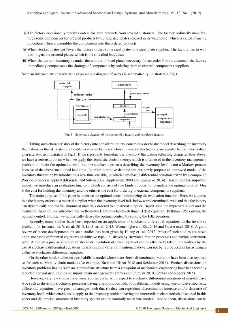
2.3. Improved model of inventory fluctuationIn order to remove the problem indicated in the previous section, we introduce a new time variable t which measures

the elapsed time except for lead time of the ordinary order, i.e., the difference between t and t corresponds to the cumulativelength of the lead time.We call the time variables t in the previous section and t in this section actual time variable andanalytic time variable, respectively. Similarly, the model in the previous section and the improved model in this sectionare called actual time model and analytic time model, respectively.

Figure 2 is a schematic diagram of each sample behavior of the inventory process in the actual time model (Fig.2(a))and the newly introduced analytic time model (Fig.2(b)). A similar approach compressing lead times is reported by Jianget.al. 2015. In what follows, we use t as a time variable.

lead time

(a) actual time model (b) analytic time model

ordinary ordermaterials arrivalXt Xt

~~

b b

t~

t

Fig. 2 Schematic diagram of each sample behavior of the inventory process in the actual time model and theanalytic time model.

Corresponding to the time variable changing from t to t, we introduce some new stochastic processes related to theinventory fluctuation. Let Ct be the cumulative amount of materials needed for customer orders arriving in the time exceptfor lead times up to time t. Since increments of C(c)

t are independent of the past, Ct can be expressed as

Ct =N(c)

t∑k=1

Yk , (5)

where N(c)t is a Poisson process with the same intensity λ as N(c)

t and Yk denotes the amount of materials required bythe k-th (counted in the time except for lead time) customer order and {Yk}k=1,2,··· is a sequence of i.i.d. positive randomvariables whose probability distribution is the same as that of {Yk}k=1,2,···. Further, let Ht be the ordinary order size processunder the new setting of time t, i.e., the factory makes an ordinary order with an ordering size Ht when the inventory levelfalls below b at time t. Let Nt be the total number of ordinary orders up to time t, which is a stochastic process that is fullydependent on the compound process Ct.

In order to take customer order behavior into the analytic time model, we newly introduce the following quantity.We assume that the length of lead time of the ordinary order depends only on how much amount of materials the factory

4



orders and let L(h0) be the length of lead time under its ordering size h0. Further, stochastic temporal variation of theinventory level within a lead time is caused only by the customer order, which is an external noise. Thus, letting Ξ be theinventory level at the end of a lead time (i.e., at the time when ordinary order arrives at the warehouse), we can express itas Ξ(x, h0) under the condition that the inventory level is x when the factory makes ordinary order and the ordering size ish0, which can be described as follows;

Ξ(x, h0) =(x −

∫ L(h0)

0dZt

)(+), (6)

where Zt is a compound Poisson process which has the same stochastic property as C(c)t and (x)(+) ≡ max{x, 0}. However,

using the expression Eq.(6), we have a serious difficulty to derive optimal control in applying the stochastic controltheory. Hence, we approximately evaluate it in terms of an expected variation of the customer order process, i.e., weredefine Ξ(x, h0) as

Ξ(x, h0) =(x − E

{∫ L(h0)

0dZt

∣∣∣h0 : given})(+). (7)

We denote an inventory process under the new time variable t by Xt, whose evolution is described by the followingstochastic differential equation;

dXt = −dCt −{Xt− − Ξ(Xt− − dCt,Ht−)

}dNt + Ht−dNt + dCtdNt, (8)

where the first, second and third terms in the right-hand side represent decrease of inventory due to customer order,decrease of inventory during the lead time and increase of inventory due to ordinary order, respectively. The forth term inthe right-hand side needs to be introduced so that the first term must be removed when the ordinary order occurs. Here,we define a constant xmax as

xmax = suph0∈[b,Hmax]

{h0 + sup

x≤b{Ξ(x, h0)}

}, (9)

which gives the upper bound of the inventory level in our model. If we suppose that the initial inventory level X0 satisfiesX0 ≤ xmax, we can easily show that an inequality Xt ≤ xmax (∀t ≥ 0) holds. Hence, we assume X0 ≤ xmax in what follows.

Let us consider temporal behavior in a time interval [s,T ] (0 ≤ s ≤ T ) and let H = {Ht; s ≤ t ≤ T } be total behaviorof the ordinary order size process in the interval. Since the solution process Xt as well as the process Nt describingordinary oder occurrences generally depend on the total variation of the ordinary order, such dependence should be takeninto notations. Thus, we newly introduce XH

t representing the solution process under the effect of H and NHt representing

the ordinary order occurrence under the effect of H. Further, we rewrite Eq.(8) as follows;

dXHt = −dCt −

{XH

t− − Ξ(XHt− − dCt,Ht−)

}dNH

t + Ht−dNHt + dCtdNH

t . (10)

It should be noted that the solution of Eq.(10)) is defined as satisfying the following stochastic integral equation;

XHt = XH

s −∫ t

sdCr −

∫ t

s

{XH

r − Ξ(XHr− − dCr,Hr−)

}dNH

r +∫ t

sHr−dNH

r +∫ t

sdCrdNH

r . (11)

Since both of Ct and NHt show only discrete jumps, Eq.(12) can be rewritten as

XHt = XH

s −∑

s<r≤tCr −

∑s<r≤t

{XH

r− − Ξ(XHr− − ∆Cr,Hr−)

}∆NH

r +∑

s<r≤tHr−∆NH

r +∑

s<r≤t∆Cr∆NH

r , (12)

where ∆Cr = Cr −Cr−, ∆NHr = NH

r −NHr− and summation is taken for all discrete jumps occurred in the time interval (s, t].

2.4. Formulation of the optimal ordinary order controlAs mentioned earlier, we suppose that the factory can dynamically control the ordinary order size, described by the

process Ht, so that it can obtain the best performance.The performance is usually quantified as costs necessary for thefactory managing its inventory level. We consider two kinds of cost: one is the cost which is spent for the factory holdingmaterials in the warehouse and the other is the cost for urgent orders. The former cost is the so-called holding cost andwe call the latter cost urgent cost. Then, we introduce the following evaluation function to quantify the performance ofordinary order size control;

JH(s, x) = Es,x{KH(s, x)}, (13)

5



where Es,x{ · } = E{ · |XHs = x} and

KH(s, x) =∫ T

sG(XH

t )dt +∫ T

sG(u)(dCt − XH

t−)dNHt +

∫ T

sβ(XH

t− − dCt,Ht−)dNHt (14)

where our control is supposed to be executed in the time interval [s,T ]. We call the total behavior H in [s,T ] simply acontrol hereinafter. In Eq.(14)), the first term of the right hand side is the total holding cost in the time except for leadtimes. The second term is the total urgent cost due to urgent orders caused by customer orders at the time of ordinaryorders. The third term is the total cost in lead times, which consists of both the holding cost and the urgent cost. Thefunctions G(x) and G(u)(y) express costs per unit time for the factory holding its inventory level x and costs for an urgentorder whose size is y respectively, which satisfy

G(x) ≡ 0 (for ∀x ≤ 0), G(u)(y) ≡ 0 (for ∀y ≤ 0). (15)

The random variable β(x, h0) represents costs in a lead time provided that the factory has made the ordinary order withsize h0 and the inventory level has been x at that time. Hence, we can express β(x, h0) as

β(x, h0) =∫ L(h0)

0G(x − Zt)dt +G(u)(Zγ − (x)(+)) +

∫ L(h0)

(γ∧L(h0))+G(u)(dZt) , (16)

where

γ = inft{t ≥ 0 | Zt > x} . (17)

Let Eβ{ · | x, h0} be an operator to take expectation with respect to β under the condition that the factory has made theordinary order with size h0 and the inventory level has been x at that time. Then, the expectation of the third term of theright hand side in Eq.(14) can be express as

Es,x{ ∫ T

sβ(XH

t− − dCt,Ht−)dNHt

}= Es,x

{ ∫ T

sEβ{β(XH

t− − dCt,Ht−) | XHt− − dCt,Ht−}dNH

t

}. (18)

Therefore, we can replace β(x, h0) by its expectation with respect to the random behavior in the lead time, denoted byβ(x, h0), i.e., Eq.(14) can be replaced as follows;

KH(s, x) =∫ T

sG(XH

t )dt +∫ T

sG(u)(dCt − XH

t−)dNHt +

∫ T

sβ(XH

t− − dCt,Ht−)dNHt . (19)

We define the optimal control H∗, which minimizes the evaluation function given by Eq.(13), as follows;

JH∗ (s, x) = infH

JH(s, x) ≡ V(s, x). (20)

2.5. Markov controlSince we improve the mathematical model of the inventory process so that the inventory process XH

t is a Markovprocess if Ht is a so-called Markov control, we consider only Markov controls in deriving the optimal control hereinafter.That is, we do not need to examine controls that depend on all the past information on the inventory system, i.e., we haveonly to examine controls that are determined by the current information. Hence, by the use of a deterministic function h,Ht is assumed to be expressed as

Ht = h(t, Xht ) , (21)

where Xht means the inventory process under the Markov control by the use of h, simply called Markov control h, which

is given as a solution of the following stochastic differential equation;

dXht = −dCt −

{Xh

t− − Ξ(Xht− − dCt, h(t−, Xh

t−))}

dNht + h(t−, Xh

t−)dNht + dCtdNh

t . (22)

In what follows, we use a notation, for example, Jh(s, x) instead of JH(s, x) provided that the control is restricted toa Markov control described by a function h(s, x).

6



3. HJB equation for optimal control3.1. Necessary condition for the optimality

To find the optimal control, we first derive a necessary condition for the optimality by applying the well-knownBellman principle.

Suppose that the optimal control H∗t is given. We define a control Ht as

Ht =

h0 for s ≤ t < s + ∆sh∗(t, Xt) for s + ∆s ≤ t ≤ T ,

(23)

with a smallness interval ∆s and an arbitrary constant h0 ∈ [b,Hmax]. Because of the optimality, the evaluation functionunder Ht, denoted by JH(s, x) can not be smaller than the evaluation function under the optimal control V(s, x), i.e., aninequality JH(s, x) ≥ V(s, x) holds, which leads to

lim∆s→0

JH(s, x) − V(s, x)∆s

≥ 0. (24)

Minimization of the left hand side in Eq.(24), the inequality is reduced to an equality as

infh0 ∈[b,Hmax]

lim∆s→0

JH(s, x) − V(s, x)∆s

= 0. (25)

Using the Bayes formula, we can obtain the following relation within first order of ∆s;

JH(s, x) = Es,x{KH(s, x)|A0}P(A0) + Es,x{KH(s, x)|A1}P(A1)

+Es,x{KH(s, x)|A2}P(A2) + Es,x{KH(s, x)|A3}P(A3) + o(∆s), (26)

where events Ai (i = 0, 1, 2, 3) mean as follows;A0 : No customer order occurs in [s, s + ∆s]A1 : One customer order occurs and an ordinary order is not made in [s, s + ∆s]A2 : One customer order occurs and an ordinary order is made in [s, s + ∆s]A3 : More than two customer orders occur in [s, s + ∆s]

Substituting Eq.(26) into Eq.(25) and calculating the left hand side of Eq.(24) (see, for example, Højgaard 2002 orØksendal and Sulem 2009), we can finally obtain the following equation;

infh∈[b,Hmax]

G(x) − λV(s, x) +∂V∂s

(s, x) + λ∫ x−b

0V(s, x − y)dF(y) + λ

∫ ∞x

G(u)(y − x)dF(y)

+λ∫ ∞

x−bβ(x − y, h)dF(y) + λ

∫ ∞x−b

V(s, h + Ξ(x − y, h))dF(y)

= 0 , (27)

where F(·) is a probability distribution function of each customer order size. Equation (27) is called HJB (Hamilton-Jacobi-Bellman) equation.

According to the cost function given by Eq.(19), we can easily derive the following terminal condition for V(s, x);

lims→T

V(s, x) = 0 . (28)

In this paper, the existence of the solution of the HJB equation (27) is verified through numerical approach in Section 4.

3.2. Sufficient condition for the optimalityNext, we show that the HJB equation also gives a sufficient condition for the optimality.Suppose that W(s, x) is a solution of the HJB equation (27) satisfying the terminal condition Eq.(26), provided that

W(s, x) is differentiable with respect to s and integrable so that integral terms in Eq.(27) exist. We construct a stochasticprocess Dt as

Dt = W(t, Xht )+

∫ t

sG(Xh

r )dr+∑

s<r≤tG(u)(∆Cr−Xh

r−)∆Nhr +

∑s<r≤tβ(Xh

r−−∆Cr, h(r, Xhr−))∆Nh

r (s ≤ t ≤ T ) ,(29)

7



where Xhs is assumed to be equal to x. Applying the well-known Ito formula (Ito 1942) for an increment of Dt, we obtain

DT − Ds =∫ T

s

∂

∂sW(r, Xh

r )dr +∑

s<r≤T∆W(r, Xh

r ) +∫ T

sG(Xh

r )dr

∑s<r≤T

G(u)(∆Cr − Xhr−)∆Nh

r +∑

s<r≤Tβ(Xh

r− − ∆Cr, h(r, Xhr−))∆Nh

r , (30)

Taking expectation of Eq.(30) by paying attention to that a jump of Cr in (r, r+ dr] occurs with probability λdr, we obtain

Jh(s, x) −W(s, x) = E{ ∫ T

sQh

r (s, x; W)dr}, (31)

where

Qhr (s, x; W) = G(Xh

r ) − λW(r, Xhr−) +

∂

∂sW(r, Xh

r ) + λ∫ Xh

r−−b

0W(r, Xh

r− − y)dF(y) + λ∫ ∞

Xhr−

G(u)(y − Xhr−)dF(y)

+λ∫ ∞

Xhr−−bβ(Xh

r− − y, h(r, Xhr−))dF(y) + λ

∫ ∞Xh

r−−bW(r, h(r, Xh

r−) + Ξ(Xhr− − y, h(r, Xh

r−)))dF(y) . (32)

Since W(s, x) is a solution of Eq.(25), an inequality Qhr (s, x; W) ≥ 0 holds for any function h(s, x) specifying a correspond-

ing Markov control. Therefore, we can conclude that W(s, x) equals to infh Jh(s, x), i.e., W(s, x) coincides with V(s, x)and a control obtained as a solution of the HJB equation gives an optimal control.

3.3. Basic algorithm for solving HJB equationIn this paper, we discuss an optimal control based upon a numerical solution of the HJB equation. To construct

a numerically solving algorithm for Eq.(25), we rewrite Eq.(25), by paying attention to that the derivative ∂V/∂s isindependent of the control variable h, as

∂V∂s

(s, x) = −G(x) + λV(s, x) − λ∫ x−b

0V(s, x − y)dF(y) − λ

∫ ∞x

G(u)(y − x)dF(y)

− infh∈[b,Hmax]

λ ∫ ∞x−bβ(x − y, h)dF(y) + λ

∫ ∞x−b

V(s, h + Ξ(x − y, h))dF(y)

. (33)

Approximating the left hand side by the use of a backward difference scheme with a small mesh size ∆s, we can obtainthe following backward recurrence formula;

V(s − ∆s) = V(s) +[G(x) − λV(s, x) + λ

∫ x−b

0V(s, x − y)dF(y) + λ

∫ ∞x

G(u)(y − x)dF(y)]∆s

+ infh∈[b,Hmax]

λ ∫ ∞x−bβ(x − y, h)dF(y) + λ

∫ ∞x−b

V(s, h + Ξ(x − y, h))dF(y)

∆s. (34)

Starting from the terminal condition given by Eq.(26), we can calculate V(s, x) by the use of Eq.(34).

4. Numerical examples

In this section, we give some numerical examples to examine optimal controls of the inventory by solving the HJBequation given by Eq.(25) based upon the recurrence formula derived in Section 3.3.

In what follows, we fix the intensity λ of the Poisson process N(c)t as λ = 1, i.e., we select a time variable so that

mean customer orders in unit time is unity. Further, we assume the probability distribution function of customer ordersize F(y) as an exponential distribution, i.e.,

F(y) =

1 − exp(− 1µy) for y ≥ 0

0 for y < 0 ,(35)

where µ is a positive constant representing mean size of each customer order. Similarly as selecting the time variable, wefix µ as µ = 1, i.e., inventory level is here supposed to be dimensionless by a normalization by the mean size of customerorder.

Based upon such setting, we fix the expiration time T and the upper bound of ordinary order size Hmax as T = 100.0,and Hmax = 30.0, respectively. The function of the holding cost G(·) is supposed to be the following bi-linear form;

G(x) =

0 for x ≤ 0g1x for 0 < x ≤ xG

g2(x − xG) + g1xG for xG < x ,(36)

8



where xG, g1 and g2 are positive constants satisfying b < xG < xmax and g1 < g2. The supposed function means that thefactory incurs higher cost for excess inventory larger than xG. We further suppose that the function of cost for an urgentorder G(u)(·) is linear, i.e.,

G(u)(y) = 0 for y ≤ 0g(u)y for y > 0 ,

(37)

where g(u) is a positive constant. Here, we fix the above constants as

g1 = 0.01, g2 = 0.02, xG = 20.0, g(u) = 0.5.

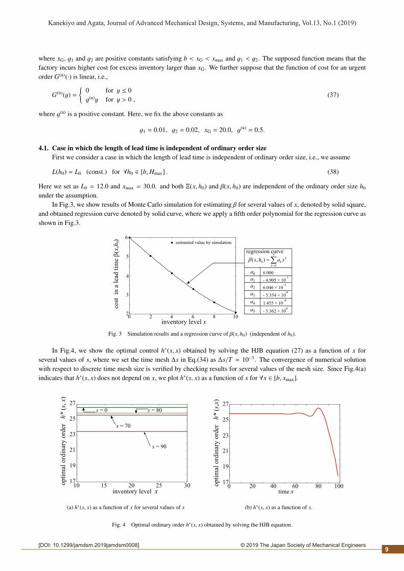
4.1. Case in which the length of lead time is independent of ordinary order sizeFirst we consider a case in which the length of lead time is independent of ordinary order size, i.e., we assume

L(h0) = L0 (const.) for ∀h0 ∈ [b,Hmax] . (38)

Here we set as L0 = 12.0 and xmax = 30.0. and both Ξ(x, h0) and β(x, h0) are independent of the ordinary order size h0

under the assumption.In Fig.3, we show results of Monte Carlo simulation for estimating β for several values of x, denoted by solid square,

and obtained regression curve denoted by solid curve, where we apply a fifth order polynomial for the regression curve asshown in Fig.3.

6

cost

in

a l

ead

tim

e β

(x,h

) 0

5

4

3

26 8 10420

estimated value by simulation

inventory level x

regression curve5

0

0

( , ) k

k

k

x h a xβ=

=∑

a5

a0

a1

a2

a3

a4

6.000

- 4.905 × 10-1

6.046 × 10-3

- 5.354 × 10-4

- 5.362 × 10-6

1.455 × 10-4

Fig. 3 Simulation results and a regression curve of β(x, h0) (independent of h0).

In Fig.4, we show the optimal control h∗(s, x) obtained by solving the HJB equation (27) as a function of x forseveral values of s, where we set the time mesh ∆s in Eq.(34) as ∆s/T = 10−3. The convergence of numerical solutionwith respect to discrete time mesh size is verified by checking results for several values of the mesh size. Since Fig.4(a)indicates that h∗(s, x) does not depend on x, we plot h∗(s, x) as a function of s for ∀x ∈ [b, xmax].

17

19

21

23

25

27

10 15 20 25 30op

tim

al o

rdin

ary

ord

er

h*

(s,

x)

inventory level x

s = 0

s = 70

s = 80

s = 90

(a) h∗(s, x) as a function of x for several values of s

0 100 17

19

21

23

25

27

op

tim

al o

rdin

ary

ord

er

h*

(s,x

)

40 20 60 80time s

(b) h∗(s, x) as a function of s.

Fig. 4 Optimal ordinary order h∗(s, x) obtained by solving the HJB equation.

9



Although Fig.4(a) shows that the optimal control h∗(s, x) is independent of x, it depends on time s only in the regionin which the rest time T − s is relatively small as shown in Fig.4(b). Further, we can see that the optimal control h∗(s, x)shows slightly oscillating behavior for 50 ≲ s ≲ 90. Here, we should note that costs in a lead time is immediately addedwithout the elapse of the lead time with respect to analytic time t. Therefore, we can expect that the optimal control tendsto reduce the frequency of ordinary orders so that the factory can reduce the total costs due to lead times. When time sbecomes close to the expiration time T , i.e., 80 ≲ s ≲ 100 in Fig.4(b), h∗(s, x) monotonically decreases as s increases sothat no ordinary order occurs after s.

On the other hand, when s is slightly smaller than 80, h∗(s, x) shows slightly increasing behavior as a function of s,which is considered to be due to a kind of balance between the costs in lead times and the holding costs. It is clear that ifthe rest time T − s is large then we can not effectively increase the probability that no ordinary order occurs after s. Thus,the optimal control abandons reducing the total costs due to lead times for reducing the total holding costs after s, thoughwe can not necessarily assert that the factory can reduce the total holding costs by making a relatively small ordinaryorder.

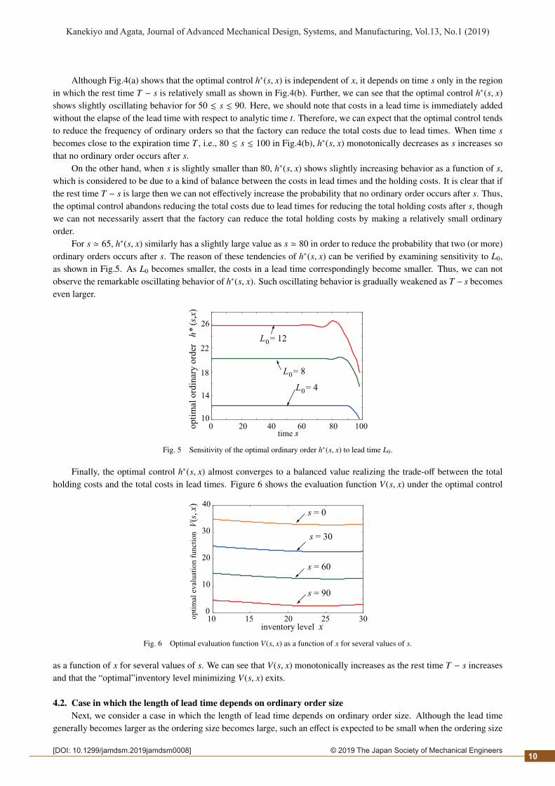
For s ≃ 65, h∗(s, x) similarly has a slightly large value as s ≃ 80 in order to reduce the probability that two (or more)ordinary orders occurs after s. The reason of these tendencies of h∗(s, x) can be verified by examining sensitivity to L0,as shown in Fig.5. As L0 becomes smaller, the costs in a lead time correspondingly become smaller. Thus, we can notobserve the remarkable oscillating behavior of h∗(s, x). Such oscillating behavior is gradually weakened as T − s becomeseven larger.

10

14

18

22

26

op

tim

al o

rdin

ary

ord

er

h*

(s,x

)

0 100 40 20 60 80time s

L = 120

L = 80

L = 40

Fig. 5 Sensitivity of the optimal ordinary order h∗(s, x) to lead time L0.

Finally, the optimal control h∗(s, x) almost converges to a balanced value realizing the trade-off between the totalholding costs and the total costs in lead times. Figure 6 shows the evaluation function V(s, x) under the optimal control

0

10

20

30

40

10 15 20 25 30inventory level x

s = 0

s = 30

s = 60

s = 90

op

tim

al e

val

uat

ion

fu

nct

ion V

(s, x)

Fig. 6 Optimal evaluation function V(s, x) as a function of x for several values of s.

as a function of x for several values of s. We can see that V(s, x) monotonically increases as the rest time T − s increasesand that the “optimal”inventory level minimizing V(s, x) exits.

4.2. Case in which the length of lead time depends on ordinary order sizeNext, we consider a case in which the length of lead time depends on ordinary order size. Although the lead time

generally becomes larger as the ordering size becomes large, such an effect is expected to be small when the ordering size

10



is small. Hence, we here assume that (i) the length of lead time is independent of ordinary order size if the ordinary ordersize is less than a threshold value and (ii) the length of lead time linearly increases as ordinary order size increases whenthe ordinary order size is larger than the threshold value, for the function L(h0), i.e., we suppose the following form;

L(h0) = L0 for b ≤ h0 < hL

l(h0 − hL) + L0 for hL ≤ h0 ≤ Hmax ,(39)

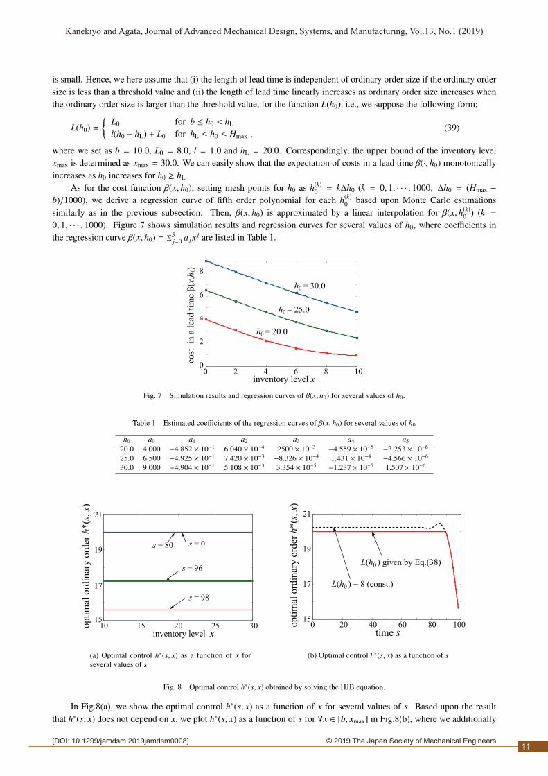
where we set as b = 10.0, L0 = 8.0, l = 1.0 and hL = 20.0. Correspondingly, the upper bound of the inventory levelxmax is determined as xmax = 30.0. We can easily show that the expectation of costs in a lead time β(·, h0) monotonicallyincreases as h0 increases for h0 ≥ hL.

As for the cost function β(x, h0), setting mesh points for h0 as h(k)0 = k∆h0 (k = 0, 1, · · · , 1000; ∆h0 = (Hmax −

b)/1000), we derive a regression curve of fifth order polynomial for each h(k)0 based upon Monte Carlo estimations

similarly as in the previous subsection. Then, β(x, h0) is approximated by a linear interpolation for β(x, h(k)0 ) (k =

0, 1, · · · , 1000). Figure 7 shows simulation results and regression curves for several values of h0, where coefficients inthe regression curve β(x, h0) = ∑5

j=0 a jx j are listed in Table 1.

0

2

4

6

8

0 2 4 6 8 10

h = 20.00

h = 25.00

h = 30.00

cost

in

a l

ead

tim

e β

(x,h

) 0

inventory level x

Fig. 7 Simulation results and regression curves of β(x, h0) for several values of h0.

Table 1 Estimated coefficients of the regression curves of β(x, h0) for several values of h0

h0 a0 a1 a2 a3 a4 a5

20.0 4.000 −4.852 × 10−1 6.040 × 10−4 2500 × 10−3 −4.559 × 10−5 −3.253 × 10−6

25.0 6.500 −4.925 × 10−1 7.420 × 10−3 −8.326 × 10−4 1.431 × 10−4 −4.566 × 10−6

30.0 9.000 −4.904 × 10−1 5.108 × 10−3 3.354 × 10−5 −1.237 × 10−5 1.507 × 10−6

op

tim

al o

rdin

ary

ord

er h

*(s

, x)

15

17

21

19


s = 0s = 80

s = 96

s = 98

(a) Optimal control h∗(s, x) as a function of x forseveral values of s

15

17

19

21

0 20 40 60 80 100op

tim

al o

rdin

ary

ord

er h

*(s

, x)

time s

L(h ) = 8 (const.)0

L(h ) given by Eq.(38)0

(b) Optimal control h∗(s, x) as a function of s

Fig. 8 Optimal control h∗(s, x) obtained by solving the HJB equation.

In Fig.8(a), we show the optimal control h∗(s, x) as a function of x for several values of s. Based upon the resultthat h∗(s, x) does not depend on x, we plot h∗(s, x) as a function of s for ∀x ∈ [b, xmax] in Fig.8(b), where we additionally

11



op

tim

al e

val

uat

ion

fu

nct

ion V

(s, x)

0

10

20

30


s = 0

s = 30

s = 60

s = 90

Fig. 9 Optimal evaluation function V(s, x) as a function of x for several values of s.

plot h∗(s, x) obtained in the case of L(h0) = 8.0 (const.), denoted by dashed curve, for comparison. Further in Fig.9, theoptimal evaluation function V(s, x) is plotted as a function of x for several values of s. As shown in Fig.8(b), there isa remarkable difference between numerical results in the previous subsection and those in this subsection. That is, theoptimal control h∗(s, x) is bounded by hL, which indicates that we should not select an ordinary order size larger than hL

so that the expected costs in a lead time is reduced.

5. Conclusions

In this paper, we have newly constructed a mathematical model using a non diffusive stochastic differential equationfor discussing the inventory management problem of a factory having effects of lead times in replenishing the inventory,in which a Markov property can be realized by effectively introducing a concept of analytical time. Consequently, wehave clarified that a technique of Markov control can be applied to such an inventory problem and thus the HJB equationcan be formulated to derive the optimal control of the ordering size for an evaluation function expressing the expectedtotal costs.

Through numerical examples, we have shown that (i) The optimal control h∗(s, x) is almost independent of an in-ventory level x just before an ordinary order, (ii) The optimal ordinary order size drastically decreases as the rest time upto the expiration time becomes small and (iii) There exists an ‘optimal’inventory level minimizing the optimal evaluationfunction.

We have clarified that the stochastic control approach can be applied to a probabilistic inventory model using stochas-tic differential equations driven by a compound Poisson process, where the HJB equation is derived and numericallysolved. Combining our result with results using diffusive model obtained so far, we can extend our discussion to moreextended and generalized probabilistic inventory models, since stochastic processes having independent increments canbe constructed as a sum of diffusive noise and a superposition of compound Poisson processes. That is, such a featureenables us to construct a probabilistic inventory model using stochastic differential equations driven by noise of moregeneral type, which has a very important meaning in the point that the discussion given by this paper can be applied toinventory problems of various types. Further, we should discuss a new mathematical model in which the factory can alsodynamically control the threshold level b in addition to its size.

References

Applebaum, D., Levy Processes and Stochastic Calculus (2009), Cambridge Univ. Press.Bellman, R., Dynamic programming (1957), Princeton Univ. Press.Chen, L., Feng, Y. and Ou, J., Joint Management of Finished Goods Inventory and Demand Process for a Make-to-Stock

Product: A Computational Approach, IEEE Transactions on Automatic Control, Vol.52, No.2 (2006), pp.258-273.Fatrias, D. and Y. Shimizu, Multi-objective analysis of periodic review inventory problem with coordinated replenishment

in two-echelon supply chain system through differential evolution, J. of Advanced Mechanical Design, Systems, andManufacturing, Vol.4, No.3 (2010), pp.637-650.

Feng, K. and Rao, U. S., Echelon-stock (R, nT ) control in two-stage serial stochastic inventory systems, OperationsResearch Letters, Vol.35 (2007), 95-104.

12



Grewal, C. S., S. T. Enns and P. Rogers, Duynamic reorder point replenishment strategies for a capacitated supply chainwith seasonal demand, Computers & Industrial Engineering, Vol. 80 (2015), pp.97-110.

Huang, J., M. Leng and L. Liang, Recent developments in dynamic advertising research, European J. of OperationalResearch, Vol. 220 (2012), pp.591-609.

Højgaard, B., Optimal dynamic premium control in non-life insurance. Maximizing dividend payouts, Scandinavian Ac-tuarial Journal, Vol. 4 (2002), pp. 225-245.

Ito, K., On Stochastic processes II: infinitely divisible laws of probability, Japanese Journal of Mathematics, Vol.18 (1942),pp.261-301.

Jian, M., X. Fang, L.-q. Jin and A. Rajapov, The impact of lead time compression on demand forecasting risk andproduction cost: A newsvendor model, Transportation Research, Part E, Vol. 84 (2015), pp.61-72.

Kanekiyo, H., Proposal of a New Probabilistic Model for Random Fatigue Crack Growth Using a Noise of Poisson Type,Journal of The Society of Materials Science, Japan, Vol.63, No.2 (2014), pp.92-97 (in Japanese).

Li, S., J. Zhang and W. Tang, Joint dynamic pricing and inventory control policy for a stochastic inventory system withperishable products, Int. J. Production Research, Vol. 53, No.10 (2015), pp.2937-2950.

Li, Y., S. Zhang and J. Han, Dynamic pricing and periodic ordering for a stochastic inventory system with deterioratingitems, Automatica, Vol. 76 (2017), pp.200-213.

Nasr, W. W. and I. J. Elshar, Continuous inventory control with stochastic and non-stationary Markovian demand, Euro-pean J. of Operational Research, Vol. 270 (2018), pp.198-217.

Øksendal, B. and A. Sulem, Applied Stochastic Control of Jump Diffusions (2007), Springer-Verlag, Berlin Heidelberg.Ouaret, S., J.-P. Kenne and A. Gharbi, Production and replacement policies for a deteriorating manufacturing system

under random demand and quality, European J. of Operational Research, Vol. 264 (2018), pp.623-636.Rempała, R., A continuous production-inventory problem with regeneration cycles, International Journal of Production

Economics, Vol.93-94 (2005), pp.447-454.Schlosser, R. Joint stochastic dynamic pricing and advertising with time-dependent demand, J. of Economic Dynamics &

Control, Vol. 73 (2016), pp.439-452.Weerasinghe, A. and C. Zhu, Optimal inventory control with path-dependent cost criteria, Stochastic Processes and their

Applications, Vol. 126 (2016), pp.1585-1621.

13

Documents

Optimal control in an inventory management problem