A

mdarTl©

K

1

MpCasScflctbSoa

sf

t(

0d

Journal of Materials Processing Technology 189 (2007) 182–191

Optimal control of induction heating for semi-solidaluminum alloy forming

H. Jiang, T.H. Nguyen, M. Prud’homme ∗Department of Mechanical Engineering, Ecole polytechnique de Montreal, C.P. 6079, Succ. Centre-ville, Montreal, Que. H3C 3A7, Canada

Received 23 February 2006; received in revised form 17 January 2007; accepted 23 January 2007

bstract

The thixoforming technique requires reheating the feedstock to a semi-solid state with a uniform temperature distribution, a uniform globularicrostructure and an optimum liquid fraction. The presence of the skin effect during induction heating results in an exponential heat source

istribution within the material as well as an uneven temperature profile from surface-to-core. In this study, the conjugate gradient method withdjoint equations is used to find an optimal heating/cooling strategy to achieve uniform temperature distribution along the radius of a cylinder in a

elatively short time. It is found that a modified conjugate gradient method may be a more suitable algorithm to solve this optimization problem.he physical and mathematical models take into account the temperature-dependent thermo-physical properties. Radiative and convective heat

osses are also considered. 2007 Elsevier B.V. All rights reserved.

lvatot

msctna

ept

eywords: Thixoforming; Heating; Optimization

. Introduction

Semi-solid metal (SSM) forming, originally introduced byerton C. Flemings at MIT in the 1970s, has become a com-

etitive technique to produce parts for the automotive industry.ompared with conventional methods like gravity die-castingnd squeeze casting, which are prone to generate various flawsuch as blowholes, segregation, and thermal defects of the die,SM requires heating the work piece to the semi-solid state withoexisting liquid and solid phases. It has the ability to increaseow viscosity and decrease the processing temperature duringasting process, resulting in laminar flow and lower solidifica-ion shrinkage and therefore a higher quality of cast productsy preventing the entrapment of gas. Additional advantages ofSM include excellent surface quality, high strength, low levelf porosity, fine microstructure of the product, energy saving,nd respect of tight tolerances [1–5].

The technique usually requires reheating pre-processed feed-tock with a fine and non-dendritic structure up to a typical liquidraction of about 40–50%. For such liquid fractions, the rheo-

∗ Corresponding author.E-mail addresses: hui.jiang@polymtl.ca (H. Jiang),

he-hung.nguyen@polymtl.ca (T.H. Nguyen), miprud@meca.polymtl.caM. Prud’homme).

fAtdtafa

924-0136/$ – see front matter © 2007 Elsevier B.V. All rights reserved.oi:10.1016/j.jmatprotec.2007.01.020

ogical properties of the semi-solid alloys are very sensitive toariations in the liquid phase. So the heating process must beccurately controlled to achieve a uniform temperature distribu-ion in the material and, in turn, in the liquid fraction. On thether hand, the heating process is required to be relatively rapido maintain the initial globular microstructure [6–7].

Induction heating is nowadays the most commonly usedethod in commercial production applications, especially in

emi-solid metal processing because it is a non-contact, clean,ompact and fast method and the input power can be easily con-rolled. However, induction heating has its inherent drawback ofon-uniform heating due to the so-called skin effect, end effectnd electromagnetic transverse edge effect.

In this paper, skin effect only is considered. The other twoffects are neglected. Because of the skin effect, most of theower density and, consequently, heat source is concentrated onhe surface, and decays exponentially with depth below the sur-ace. The outside will then heat more quickly than the inside.bout 86% of the heat is generated in a surface layer called

he current penetration depth. The non-uniform temperatureistribution along the radius of the material is called the surface-

o-core temperature profile [2,8–10]. The penetration depth isfunction of frequency and material properties, decreasing as

requency increases. In order to maximize electrical efficiencynd minimize electromagnetic forces, the commercial machines

rocessing Technology 189 (2007) 182–191 183

oc

iddmeth

locfiasfimfadsfltrwOu

tpstIdSa

2

auiatmpstpmeobi

tt

2

rdaie

ρ

wttlE

C

T

I

p b p εs εp Ap

H. Jiang et al. / Journal of Materials P

ften operate at frequencies above 10 KHz. Such high frequen-ies also allow more compact systems.

If the temperature reaches some preset maximal value, thenput power is either cut or decreased. The heating procedure isetermined from experiments and/or automatic control proce-ures. However, the drawbacks are also obvious: the strategyay not be optimal, the heating time may be long, and the

xperiments must be repeated if either the size of the object,he material itself, or the operating frequency of the inductioneater is changed.

This heating control problem is essentially an inverse prob-em of determining the time-dependent heat source required tobtain a targeted temperature distribution. This kind of optimalontrol problem in a distributed-parameter system was proposedrst by Butkovskii and Lerner [11] in 1960. To solve the linearnd nonlinear boundary control problems, Sakawa [12,13] sub-equently used a variational method, Cavin and Tandon [14] anite element method, and Meric [15,16] a conjugate gradientethod. In the last two decades, the solution algorithms were

urther improved with the rapid development of optimizationnd inverse problem techniques. Kelley and Sachs [17] intro-uced a Steihaug trust region conjugate gradient method with amoothing step at each iteration to solve a 1-D boundary heatux control problem. Huang [18] solved a similar boundary con-

rol problem with temperature-dependent thermal properties byegular conjugate gradient method. The same control problemas extended to 3-D geometries by Huang and Li [19]. Chen andzisik [20,21] estimated the optimum strength of heat sourcessing an algorithm similar to Meric’s.

These optimization techniques have not yet been appliedo semi-solid forming problems. The objective of the presentaper is to determine by conjugate gradient an optimal heatingtrategy to achieve a uniform temperature distribution alonghe radius of a cylindrical billet, within a relatively short time.n this study, all thermal properties are considered temperatureependent and the heat source is a function of time and space.urface heat radiation and convection are also taken intoccount.

. Problem definition

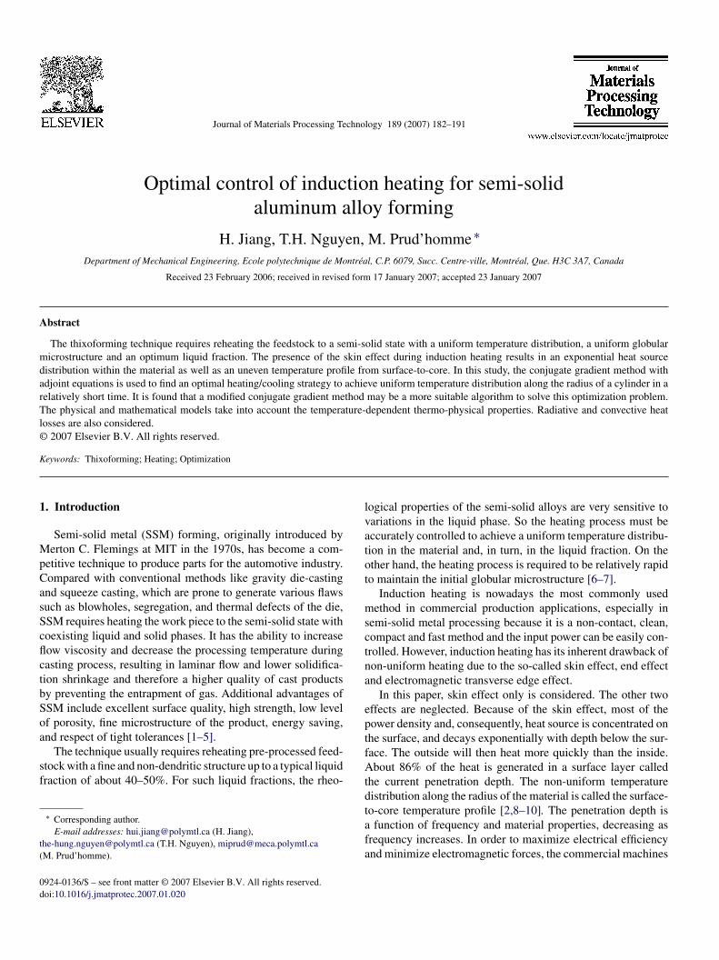
An aluminum alloy (A356) slug with a diameter of 76 mmnd a height of 152 mm is placed vertically into an induction coilnit as sketched in Fig. 1. The power supply generates alternat-ng current at 10 KHz. In order to obtain a uniform liquid fractionnd a good viscosity, the billet temperature should be kept withinhe range of 575–585 ◦C over the entire cross-section before the

aterial flows into the die cavity under pressure. Only the one-hase model is considered here, i.e., the targeted temperature iset below the melting point of the alloy. The two-phase model ishe subject of on-going research. Due to the skin effect, the tem-erature is not uniform along the radius of the billet, as Tsurfaceust be higher than Tcenter. The transverse electromagnetic edge

ffects are not considered because of the cylindrical geometryf the work-piece, and the ‘elephant foot’ effect is assumed toe controlled. If the induction heater is well designed and theres no coil overhang, then the end effects and the top-to-bottom

iTip

Fig. 1. Schematic representation of Induction Heating Coil and Slug.

hermal gradients may be ignored. The physical model can beherefore simplified to the one-dimensional case.

.1. Mathematical model

Let us consider a metal cylinder cooled by convection andadiation. The initial temperature field and the boundary con-itions are known a priori. An internal heat source which isfunction of space and time is generated by induction heat-

ng. This heat conduction problem is governed by the non-linearquation:

(T )cp(T )∂T

∂t= 1

r

∂

∂r

(k(T )r

∂T

∂r

)+ S(r, t) (1)

here S(r,t) denotes the inner heat source, ρ is the density, cphe specific heat and k the thermal conductivity. It is assumedhat the heat source may be factorized as S(r,t) = G(t)H(r) andet us introduce the volumetric heat capacity C(T) = ρ(T)cp(T).q. (1) may then be recast as:

(T )∂T

∂t= 1

r

∂

∂r

(k(T )r

∂T

∂r

)+ G(t)H(r) (2)

he corresponding boundary and initial conditions are:

k∂T

∂r

∣∣∣∣r=0

= 0, k∂T

∂r

∣∣∣∣r=R

= p(T ) + q(t), T (r, 0) = f (r) (3)

n the above, q(t) is the convective heat flux and

(T ) = σ (T 4 − T 4)

(1 + 1 − εp As

)−1

(4)

s the radiative heat flux with the Stefan-Boltzmann constant σb.he subscript ‘s’ refers to the slug surface, while ‘p’ denotes

nner surface of the heater pedestal. It is assumed that theedestal is cooled by water, and that Tp ≡ Tambient.

184 H. Jiang et al. / Journal of Materials Proc

2

ctrIodm

H

wFif

δ

FiAsIsrctm

3

btos

tt

E

ioqparas

3

d

T

Sa

Sc

T

3

t

D

I(iaa

C

sa

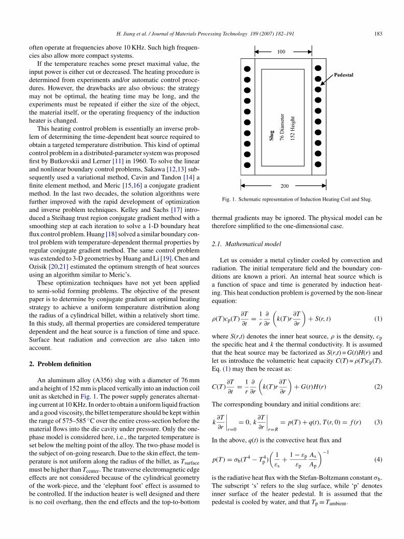
Fig. 2. Heat source distribution of A356.

.2. Heat source distribution

It can be derived from Maxwell equations that the inducedurrent density decreases exponentially from the periphery ofhe billet towards the center [22]. The distribution of cur-ent density within a cylinder-shaped material is of the form(r) = I0 exp[(r − R)/δ] where I0 is the maximum eddy currentn the surface, R the radius of the cylinder and δ the penetrationepth. From Joule’s law, the radial power density distributionay be obtained as:

(r) = H0I2

I20

= H0 e−2(R−r)/δ (5)

here H0 denotes the maximum power density on the surface.or metallic materials, δ can be expressed in terms of the resistiv-

ty χ, permeability μr of the material and the current frequencyas:

= 503.3√

χ

μrf(6)

or aluminum alloys and copper, μr ∼= 1. The load resistiv-ty is proportional to the temperature. For the aluminum alloy356, χ = 3.89 × 10−8 + 1.53 × 10−10 T (�-m). The power den-

ity distribution for A356 along the radius is shown in Fig. 2.t is found that the temperature does not influence the heatource distribution significantly within the range 20–570 ◦C. Theesistivity can be treated as a constant therefore. However, theurrent frequency considerably affects the heat source distribu-ion. Generally speaking, the temperature distribution becomes

ore uniform as the frequency decreases.

. Optimal heating control problem

According to the above discussion, the heat source distri-

ution H(r) will be determined by the operating frequency ofhe induction heater. If the surface cooling flux q(t) is given,ur objective is to determine the evolution in time of the heatource G(t) such that the final temperature T(r,tf) is equal to the

k

T

essing Technology 189 (2007) 182–191

argeted value TE(r). The solution is obtained by minimizinghe error functional E:

(G) = 1

2

∫ R

0[T (r, tf) − TE(r)]2 dr + ξ

2

∫ tf

0G2(t) dt (7)

n which ξ is a regularization parameter. Among the variousptimization techniques, the conjugate gradient method is fre-uently adopted because of its efficiency and self-regularizationroperty. As with any iterative algorithm, the search directionnd step size must be determined. The search direction iselated to the gradient of E, which is obtained by solving andjoint problem, while the optimal step size is determined byolving a sensitivity problem.

.1. Sensitivity equation

The sensitivity temperature T is defined as the directionalerivative of T at G in the direction G:

˜ = limε→0

T (G + εG) − T (G)

ε(8)

tarting from Eq. (2), the sensitivity equation is readily obtaineds:

∂(CT )

∂t= 1

r

∂

∂r

(r∂(kT )

∂r

)+ GH (9)

imilarly, one can derive the corresponding initial and boundaryonditions:

˜ (r, 0) = 0,∂(kT )

∂r

∣∣∣∣r=0

= 0,∂(kT )

∂r

∣∣∣∣r=R

= (p′T )∣∣r=R

(10)

.2. Adjoint equation

According to the definitions of the error functional and theemperature sensitivity, it follows that:

GE(G) =∫ R

0{T (r, tf)[T (r, tf) − TE]} dr + ξ

∫ tf

0(GG) dt

=∫ tf

0(∇EG) dt (11)

f the adjoint temperature T and Eq. (9) are introduced into Eq.11) as a Lagrange multiplier and as a constraint, respectively, its possible after some rearrangements and considering the initialnd boundary conditions of the sensitivity problem, to obtain thedjoint problem defined by the equation:

∂T

∂t+ k

r

∂

∂r

(r∂T

∂r

)= 0 (12)

olved backwards in time with the transformation τ = tf − t. Thessociated boundary and initial conditions are:

∂T∣∣∣∣ = 0, k

∂T∣∣∣∣ = (p′T )

∣∣r=R

,

∂r r=0 ∂r r=R

¯ (r, tf) = −T (r, tf) − TE(r)

Cr(13)

roces

T

D

Ig

3

b

G

P

Tfir

α

b

1

23456

P

β

1

3

sifiigo

ic

G

wi

Tgt

∇

Td

p

R

T(b

4

usm

E

Rb

T

Te

H. Jiang et al. / Journal of Materials P

he right-hand side of Eq. (11) then becomes:

GE(G) =∫ tf

0

(ξG −

∫ R

0THr dr

)G dt (14)

t follows by comparison of Eq. (14) with Eq. (11) that theradient of the error functional is:

E = ξG −∫ R

0T (r, t)H(r)r dr (15)

.3. Regular conjugate gradient method

The iterative formula and the conjugate search direction maye expressed as:

k+1 = Gk + αkPk (16)

k = −∇Ek + βkPk−1 (17)

he optimal step size may be determined by requiring that therst order derivative of E in the direction αk must vanish. Theesult is:

k = −∫ R

0 (T k − TE)T k dr + ξ∫ tf

0 GkPk dt∫ R

0 (T k)2 dr + ξ∫ tf

0 (Pk)2 dt(18)

The overall CGM algorithm of the Polak-Ribiere version maye summarized as follows:

. Choose an initial guess G0 = G0(t) and set the iterationcounter to k = 0.

. Solve the direct problem with Gk to obtain Tk.

. Evaluate the difference Tk(r,tf) − TE.

. Solve the adjoint problem backward in time for T k.

. Evaluate the gradient according to Eq. (15).

. Calculate the search direction Pk:

k ={

−∇Ek if k = 0

−∇Ek + βkPk−1 if k > 0(19)

k =∫ tf

0 (∇Ek − ∇Ek−1)∇Ek dt∫ tf0 (∇Ek−1)2 dt

(20)

7. Solve the sensitivity problem with G = Pk to obtain T k.8. Calculate the step size αk with Eq. (18).9. Update the guess value to Gk+1 = αkPk.0. Set k = k + 1, go back to step 2, repeat until the convergence

criterion Ek < ε is satisfied.

.4. Modified conjugate gradient method

The works presented in [17,19,23] show that the optimalolutions by regular CGM may converge over most of the timenterval to an averaged value and exhibit steep variations near the

nal time. Such a heating/cooling curve is difficult to reproduce

n engineering applications. In fact, a modification of the conju-ate direction is found to be a good way to improve the profile ofptimization solutions [24]. This modified CG method [25–28]

∇Ts

sing Technology 189 (2007) 182–191 185

s based on the assumption that the objective function G(t) is aontinuously differentiable function expressible as:

(t) =∫ t

0

dG(t′)dt′

dt′ ⇒ G(t) =∫ t

0

dG(t′)dt′

dt′ (21)

hich implies that G = G = 0 at t = 0. Differentiating under thentegral sign yields the equality:

d

dt

∫ t

tf

∫ R

0T (r, t′)H(r)rd r dt′ =

∫ R

0T (r, t)H(r)r dr (22)

his relation may be substituted back into Eq. (11). After inte-ration by parts and comparison with Eq. (14) we can concludehat:

E

(dG

dt

)= −

∫ tf

t

∫ R

0T (r, t′)H(r)r dr dt′ =

∫ tf

t∇E dt′

(23)

he modified search direction is related to the derivative of theirection of descent Rk by the formulas:

k =∫ t

0Rk dt′ (24)

k = −∇E

(dG

dt

)+ βkRk−1 (25)

he conjugate coefficient βk is still given in this case by Eq.20), where the gradient of the error function is simply replacedy the left-hand side of Eq. (23).

. Optimal cooling control problem

Let us determine the cooling flux q(t) required to achieve aniform final temperature distribution assuming that the heatource S(r,t) is known. The optimization solution is obtained byinimizing the error functional E:

(q) = 1

2

∫ R

0[T (r, tf) − TE(r)]2 dr + ξ

2

∫ tf

0q2(t) dt (26)

epeating the same procedure all over, the sensitivity problemecomes:

∂(CT )

∂t= 1

r

∂

∂r

(r∂(kT )

∂r

)(27)

˜ (r, 0) = 0,∂(kT )

∂r

∣∣∣∣r=0

= 0,∂(kT )

∂r

∣∣∣∣r=R

= (p′T )|r=R + q(t)

(28)

he adjoint problem is left unchanged, while the gradient of therror functional now becomes:

E = ξq − T (R, t)R (29)

he overall CGM algorithm remains the same as in the previousection.

186 H. Jiang et al. / Journal of Materials Processing Technology 189 (2007) 182–191

Table 1Thermo-physical and electromagnetic properties of A356

Density (kg/m3) −0.208 T (◦C) + 2680.0Specific heat (J/kg ◦C) 0.454 T (◦C) + 904.6Thermal conductivity (W/m ◦C) 0.04 T (◦C) + 153.1Solidus temperature (◦C) 555Liquid temperature (◦C) 615RR

5

ApTitmHtr

5

ta

P

I

aoGbbp

TP

CATEEME

Fc

t1

5

iat

esistivity (� m) 8.0 × 10−8

elative magnetic permeability 1.0

. Results and discussion

The solution algorithm is tested here for the specific case of356 aluminum alloy. The thermo-physical and electromagneticroperties of this light metal alloy are shown in Table 1 [7,22].he other parameters used for the calculations are presented

n Table 2. The resistivity of the material should be propor-ional to the temperature. The surface emissivity of the metal

ay vary with temperature and oxidation during the heating.owever, both parameters are treated as constants here since

heir variations would only have a minor impact on the finalesults.

.1. Optimal heating problem

In this section, the forced convection cooling flux is supposedo be known. From Eq. (5), the input power may be expresseds:

(t) = 1

ηE

∫ ∫V

∫S(x, t) dV

= G(t)

ηE

∫ H

0

∫ 2π

0

∫ R

0e−2(R−r)/δr dr dθ dz

= 2πH

ηE

(δR

2− δ2

4+ δ2

4e−2R/δ

)G(t) (30)

t follows that:

P(t)

Pmax= G(t)

Gmax(31)

It is our purpose to heat up the material to 545 ◦C as uniformlys possible. If the objective function G(t) is determined, then theptimal heating strategy, namely, P(t), is obtained. We note that

(t) should be equal to or greater than zero. This restriction muste taken into account in the optimization problem, which thenecomes a constrained minimization problem. If the maximumower of the induction heater is 9 KW and the efficiency of

able 2arameters in calculations

urrent frequency (Hz) 10,000mbient temperature (◦C) 20argeted temperature (◦C) 530 or 545missivity (aluminum alloy) 0.1missivity (ceramic pedestal) 0.94aximum input power (W) 9000

lectrical efficiency of induction heater (%) 80.0

t(wss[JlsdIadh

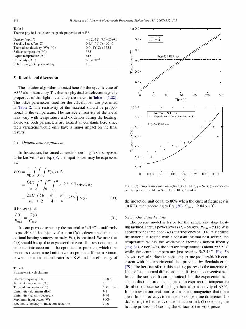
ig. 3. (a) Temperature evolution, q(t) = 0, f = 10 KHz, tf = 240 s; (b) surface-to-ore temperature profile, q(t) = 0, f = 10 KHz, tf = 240 s.

he induction unit equal to 80% when the current frequency is0 KHz, then according to Eq. (30), Gmax = 2.84 × 108.

.1.1. One stage heatingThe present model is tested for the simple one stage heat-

ng method. First, a power level P(t) = 56.85% Pmax = 5116 W ispplied to the sample for 240 s at a frequency of 10 KHz. Becausehe material is heated with a constant internal heat source, theemperature within the work-piece increases almost linearlyFig. 3a). After 240 s, the surface temperature is about 553.5 ◦Chile the central temperature just reaches 542.5 ◦C. Fig. 3b

hows a typical surface-to-core temperature profile which is con-istent with the experimental data provided by Bendada et al.29]. The heat transfer in this heating process is the outcome ofoule effect, thermal diffusion and radiative and convective heatoss at the surface. It can be noticed that the exponential heatource distribution does not yield an exponential temperatureistribution, because of the high thermal conductivity of A356.

t is known from heat transfer and electromagnetics that therere at least three ways to reduce the temperature difference: (1)ecreasing the frequency of the induction unit; (2) extending theeating process; (3) cooling the surface of the work-piece.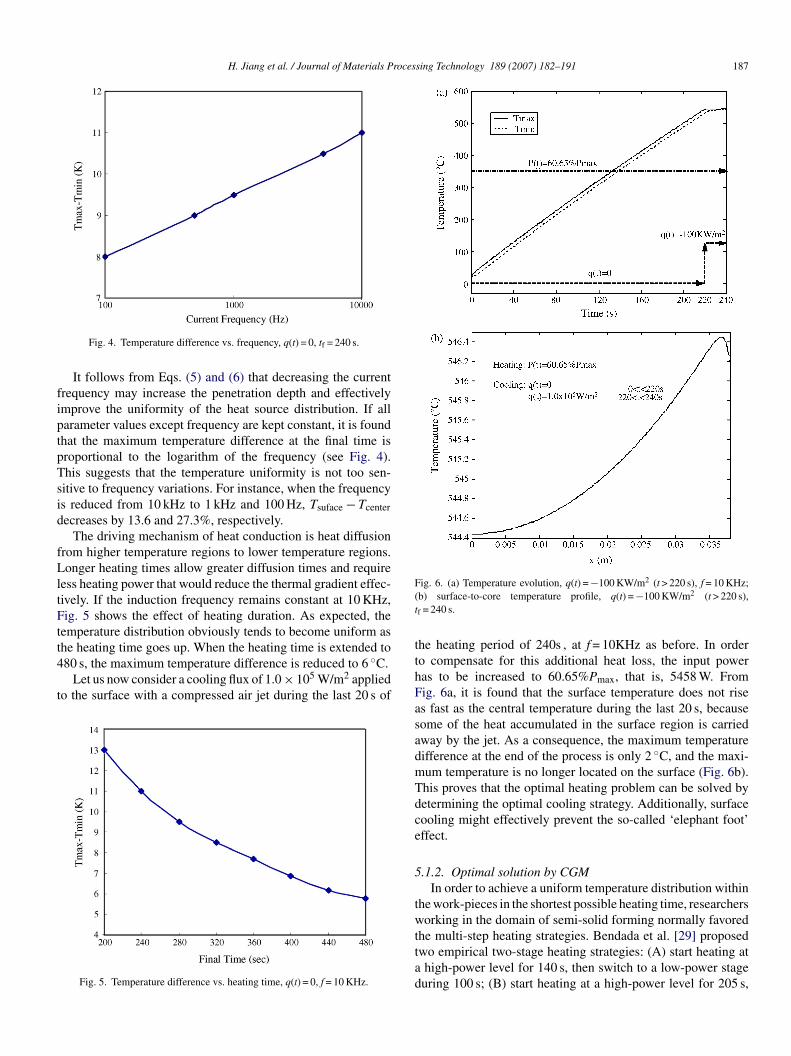

H. Jiang et al. / Journal of Materials Processing Technology 189 (2007) 182–191 187

fiptpTsid

fLltFtt4

t

F(t

Fig. 4. Temperature difference vs. frequency, q(t) = 0, tf = 240 s.

It follows from Eqs. (5) and (6) that decreasing the currentrequency may increase the penetration depth and effectivelymprove the uniformity of the heat source distribution. If allarameter values except frequency are kept constant, it is foundhat the maximum temperature difference at the final time isroportional to the logarithm of the frequency (see Fig. 4).his suggests that the temperature uniformity is not too sen-itive to frequency variations. For instance, when the frequencys reduced from 10 kHz to 1 kHz and 100 Hz, Tsuface − Tcenterecreases by 13.6 and 27.3%, respectively.

The driving mechanism of heat conduction is heat diffusionrom higher temperature regions to lower temperature regions.onger heating times allow greater diffusion times and require

ess heating power that would reduce the thermal gradient effec-ively. If the induction frequency remains constant at 10 KHz,ig. 5 shows the effect of heating duration. As expected, the

emperature distribution obviously tends to become uniform as

he heating time goes up. When the heating time is extended to80 s, the maximum temperature difference is reduced to 6 ◦C.

Let us now consider a cooling flux of 1.0 × 105 W/m2 appliedo the surface with a compressed air jet during the last 20 s of

Fig. 5. Temperature difference vs. heating time, q(t) = 0, f = 10 KHz.

tthFasadmTdce

5

twttad

ig. 6. (a) Temperature evolution, q(t) = −100 KW/m2 (t > 220 s), f = 10 KHz;b) surface-to-core temperature profile, q(t) = −100 KW/m2 (t > 220 s),

f = 240 s.

he heating period of 240s , at f = 10KHz as before. In ordero compensate for this additional heat loss, the input poweras to be increased to 60.65%Pmax, that is, 5458 W. Fromig. 6a, it is found that the surface temperature does not rises fast as the central temperature during the last 20 s, becauseome of the heat accumulated in the surface region is carriedway by the jet. As a consequence, the maximum temperatureifference at the end of the process is only 2 ◦C, and the maxi-um temperature is no longer located on the surface (Fig. 6b).his proves that the optimal heating problem can be solved byetermining the optimal cooling strategy. Additionally, surfaceooling might effectively prevent the so-called ‘elephant foot’ffect.

.1.2. Optimal solution by CGMIn order to achieve a uniform temperature distribution within

he work-pieces in the shortest possible heating time, researchersorking in the domain of semi-solid forming normally favored

he multi-step heating strategies. Bendada et al. [29] proposedwo empirical two-stage heating strategies: (A) start heating athigh-power level for 140 s, then switch to a low-power stageuring 100 s; (B) start heating at a high-power level for 205 s,

188 H. Jiang et al. / Journal of Materials Processing Technology 189 (2007) 182–191

F z, tf =( on of

tpptSe(drelbtdft

Catt

tgssz

tedsasoeec

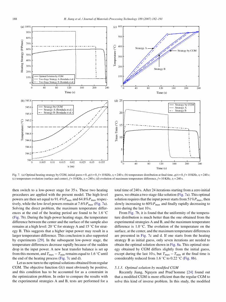
ig. 7. (a) Optimal heating strategy by CGM, initial guess = 0, q(t) = 0, f = 10 KHc) temperature evolution (surface and center), f = 10 KHz, tf = 240 s; (d) evoluti

hen switch to a low-power stage for 35 s. These two heatingrocedures are applied with the present model. The high-levelowers are then set equal to 91.4%Pmax and 64.8%Pmax respec-ively, while the low-level powers remain at 7.6%Pmax (Fig. 7a).olving the direct problem, the maximum temperature differ-nces at the end of the heating period are found to be 1.6 ◦CFig. 7b). During the high-power heating stage, the temperatureifference between the center and the surface of the sample alsoemains at a high level: 20 ◦C for strategy A and 15 ◦C for strat-gy B. This suggests that a higher input power may result in aarger temperature difference. This conclusion is also supportedy experiments [29]. In the subsequent low-power stage, theemperature differences decrease rapidly because of the suddenrop in the input power. A new heat transfer balance is set uprom this moment, and Tmax − Tmin remains equal to 1.6 ◦C untilhe end of the heating process (Fig. 7c and d).

Let us now turn to the optimal solutions obtained from regular

GM. The objective function G(t) must obviously be positive,nd this condition has to be accounted for as a constraint inhe optimization problem. In order to compare the results withhe experimental strategies A and B, tests are performed for a

5

ts

240 s; (b) temperature distribution at final time, q(t) = 0, f = 10 KHz, tf = 240 s;maximum temperature difference, f = 10 KHz, tf = 240 s.

otal time of 240 s. After 24 iterations starting from a zero initialuess, we obtain a two-stage-like solution (Fig. 7a). This optimalolution requires that the input power starts from 51%Pmax, thenlowly increasing to 60%Pmax and finally rapidly decreasing toero during the last 10 s.

From Fig. 7b, it is found that the uniformity of the tempera-ure distribution is much better than the one obtained from thexperimental strategies A and B, and the maximum temperatureifference is 1.0 ◦C. The evolution of the temperature on theurface, at the center, and the maximum temperature differencesre presented in Fig. 7c and d. If one starts from the heatingtrategy B as initial guess, only seven iterations are needed tobtain the optimal solution shown in Fig. 8a. This optimal strat-gy obtained by CGM differs slightly from the initial guess,xcept during the last 10 s, but Tmax − Tmin at the final time isonsiderably reduced from 1.6 ◦C to 0.22 ◦C (Fig. 8b).

.1.3. Optimal solution by modified CGMRecently Jiang, Nguyen and Prud’homme [24] found out

hat a modified CGM is more efficient than the regular CGM toolve this kind of inverse problem. In this study, the modified

H. Jiang et al. / Journal of Materials Processing Technology 189 (2007) 182–191 189

f = 24

aTab

Fe

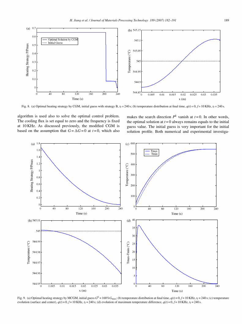
Fig. 8. (a) Optimal heating strategy by CGM, initial guess with strategy B, t

lgorithm is used also to solve the optimal control problem.he cooling flux is set equal to zero and the frequency is fixedt 10 KHz. As discussed previously, the modified CGM isased on the assumption that G = G = 0 at t = 0, which also

mtgs

ig. 9. (a) Optimal heating strategy by MCGM, initial guess G0 = 168%Gmax; (b) temvolution (surface and center), q(t) = 0, f = 10 KHz, tf = 240 s; (d) evolution of maxim

0 s; (b) temperature distribution at final time, q(t) = 0, f = 10 KHz, tf = 240 s.

akes the search direction Pk vanish at t = 0. In other words,he optimal solution at t = 0 always remains equals to the initialuess value. The initial guess is very important for the initialolution profile. Both numerical and experimental investiga-

perature distribution at final time, q(t) = 0, f = 10 KHz, tf = 240 s; (c) temperatureum temperature difference, q(t) = 0, f = 10 KHz, tf = 240 s.

1 Proc

thc

spmmltd(ihcitmpv

Fd

md

5

TsfitsotPas

90 H. Jiang et al. / Journal of Materials

ions suggest that the initial input power should be set to aigh level. The zero initial guess is then obviously not a goodhoice.

When the initial guess G0 is set equal to 168%Gmax, amooth heating control curve which requires reducing the inputower gradually from maximum to zero is predicted from theodified CGM (see Fig. 9a). The final temperature unifor-ity is perfectly achieved after 6 iterations: Tmax − Tmin is as

ittle as 0.04 ◦C (Fig. 9b). Furthermore, the surface tempera-ure also increases smoothly and the temperature variation rateT/dt monotonously decreases as the heating time increasesFig. 9c). During the last 40 s, dT/dt is very low because thenput power is almost zero. Considering the surface radiationeat loss, the surface temperature is even less than that of theenter at the final time. There is no risk of surface overheat-ng, meaning that the ‘elephant foot’ phenomenon is not likely

o occur. Comparing Fig. 9d and a, it is found that the maxi-

um temperature difference is almost proportional to the inputower. This proves again that reducing the heating power to aery low level and even to zero in the last few seconds is the

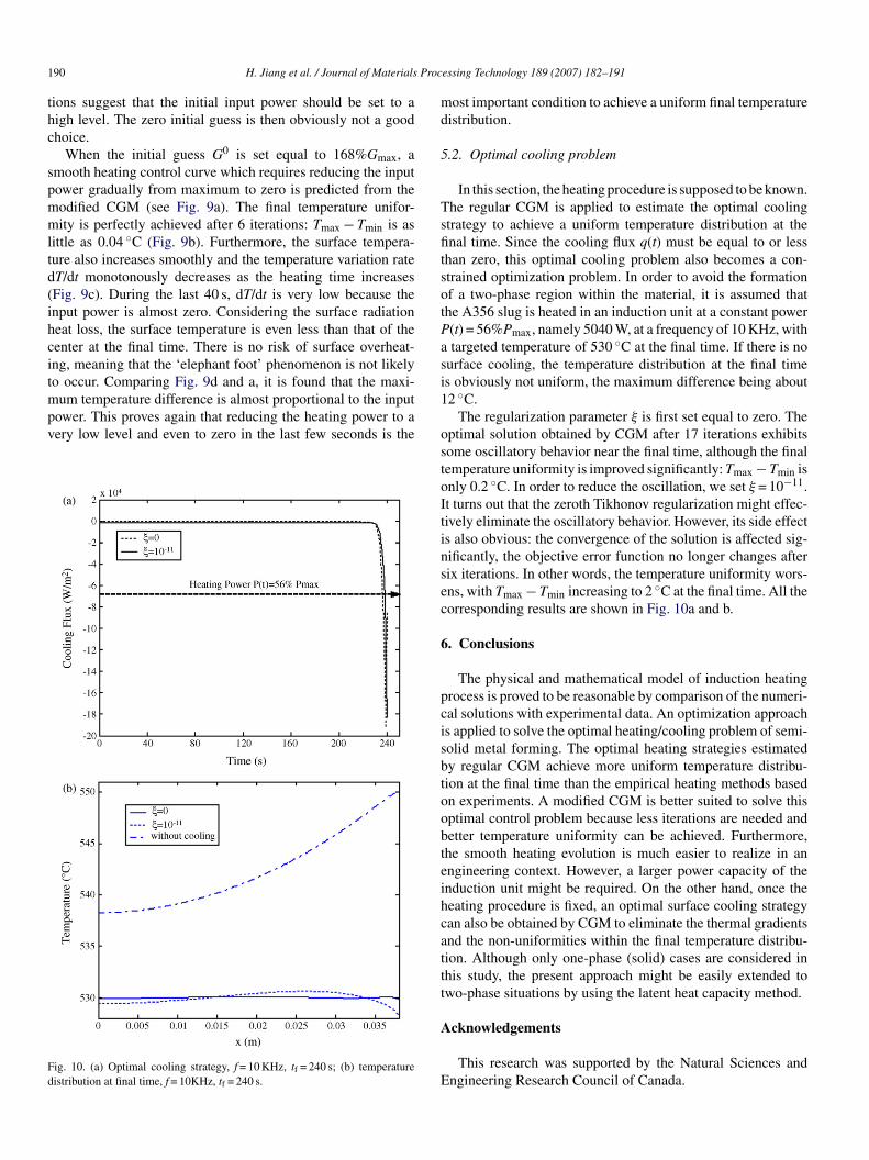
ig. 10. (a) Optimal cooling strategy, f = 10 KHz, tf = 240 s; (b) temperatureistribution at final time, f = 10KHz, tf = 240 s.

i1

ostoItinsec

6

pcisbtoobteihcattt

A

E

essing Technology 189 (2007) 182–191

ost important condition to achieve a uniform final temperatureistribution.

.2. Optimal cooling problem

In this section, the heating procedure is supposed to be known.he regular CGM is applied to estimate the optimal coolingtrategy to achieve a uniform temperature distribution at thenal time. Since the cooling flux q(t) must be equal to or less

han zero, this optimal cooling problem also becomes a con-trained optimization problem. In order to avoid the formationf a two-phase region within the material, it is assumed thathe A356 slug is heated in an induction unit at a constant power(t) = 56%Pmax, namely 5040 W, at a frequency of 10 KHz, withtargeted temperature of 530 ◦C at the final time. If there is no

urface cooling, the temperature distribution at the final times obviously not uniform, the maximum difference being about2 ◦C.

The regularization parameter ξ is first set equal to zero. Theptimal solution obtained by CGM after 17 iterations exhibitsome oscillatory behavior near the final time, although the finalemperature uniformity is improved significantly: Tmax − Tmin isnly 0.2 ◦C. In order to reduce the oscillation, we set ξ = 10−11.t turns out that the zeroth Tikhonov regularization might effec-ively eliminate the oscillatory behavior. However, its side effects also obvious: the convergence of the solution is affected sig-ificantly, the objective error function no longer changes afterix iterations. In other words, the temperature uniformity wors-ns, with Tmax − Tmin increasing to 2 ◦C at the final time. All theorresponding results are shown in Fig. 10a and b.

. Conclusions

The physical and mathematical model of induction heatingrocess is proved to be reasonable by comparison of the numeri-al solutions with experimental data. An optimization approachs applied to solve the optimal heating/cooling problem of semi-olid metal forming. The optimal heating strategies estimatedy regular CGM achieve more uniform temperature distribu-ion at the final time than the empirical heating methods basedn experiments. A modified CGM is better suited to solve thisptimal control problem because less iterations are needed andetter temperature uniformity can be achieved. Furthermore,he smooth heating evolution is much easier to realize in anngineering context. However, a larger power capacity of thenduction unit might be required. On the other hand, once theeating procedure is fixed, an optimal surface cooling strategyan also be obtained by CGM to eliminate the thermal gradientsnd the non-uniformities within the final temperature distribu-ion. Although only one-phase (solid) cases are considered inhis study, the present approach might be easily extended towo-phase situations by using the latent heat capacity method.

cknowledgements

This research was supported by the Natural Sciences andngineering Research Council of Canada.

roces

R

[

[

[

[

[

[

[

[

[

[

[

[

[

[

[

[

[

[

[

H. Jiang et al. / Journal of Materials P

eferences

[1] S. Midson, K. Brissing, Semi-solid casting of aluminum alloys: a statusreport, Mod. Cast. (1997) 41–43.

[2] S. Midson, V. Rudnev, R. Gallik, Semi-solid processing of aluminum alloys,Ind. Heat. (1999) 37–41.

[3] H.K. Jung, C.G. Kang, Induction heating process of an Al–Si aluminumalloy for semi-solid die casting and its resulting microstructure, J. Mater.Process. Technol. 120 (2002) 355–364.

[4] Y. Ono, C.Q. Zheng, F.G. Hamel, R. Charron, C.A. Loong, Experimentalinvestigation on monitoring and control of induction heating process forsemi-solid alloys using the heating coil as sensor, Meas. Sci. Technol. 13(2002) 1359–1365.

[5] D.-C. Ko, G.-S. Min, B.-M. Kim, J.-C. Choi, Finite element analysis for thesemi-solid state forming of aluminum alloy considering induction heating,J. Mater. Process. Technol. 100 (2000) 95–104.

[6] M.C. Flemings, Behavior of metal alloys in the semi-solid state, Metall.Trans. A 22 (1991) 957–981.

[7] K.T. Nguyen, A. Bendada, An inverse approach for the prediction of thetemperature evolution during induction heating of a semi-solid castingbillet, Modell. Simul. Mater. Sci. Eng. 8 (2000) 857–870.

[8] S. Midson, V. Rudnev, R. Gallik, The induction heating of semi-solid alu-minum alloys, in: Proceedings of the Fifth International Conference onSemi-Solid Processing of Alloys and Composites, Golden, CO, 1998, pp.497–504.

[9] A. Bendada, K.T. Nguyen, C.A. Loong, Application of infrared imagingin optimizing the induction heating of semi-solid aluminum alloys, in:Proceedinmgs of the International Symposium on Advanced Sensors forMetals Processing, Quebec, 1999, pp. 331–342.

10] P. Kapranos, R.C. Gibson, D.H. Kirkwood, C.M. Sellars, Induction heatingand partial melting of high melting point thixoformable alloys, in: Proceed-ings of the Fourth International Conference on Semi-Solid Processing ofAlloys and Composites, Sheffield, 1996, pp. 148–152.

11] A.G. Butkovskii, A.Y. Lerner, The optimal control systems with distributedparameter, Auto. Remote Control 21 (1960) 472–477.

12] Y. Sakawa, Solution of an optimal control problem in a distributed-parameter system, IEEE Trans. Auto. Contr. AC-9 (1964) 420–426.

13] Y. Sakawa, Optimal control of a certain type of linear distributed-parametersystem, IEEE Trans. Auto. Contr. AC-11 (1966) 35–41.

14] R.K. Cavin, S.C. Tandon, Distributed parameter system optimum con-trol design via finite element discretization, Automatica 13 (1977) 611–614.

[

sing Technology 189 (2007) 182–191 191

15] R.A. Meric, Finite element analysis of optimal heating of a slab with tem-perature dependent thermal conductivity, Int. J. Heat Mass Transfer 22(1979) 1347–1353.

16] R.A. Meric, Finite element and conjugate gradient methods for a nonlinearoptimal heat transfer control problem, Int. J. Numer. Methods Eng. 14(1979) 1851–1863.

17] C.T. Kelley, E.W. Sachs, A trust region method for parabolic boundarycontrol problems, SIAM J. Optimization 9 (1999) 1064–1081.

18] C.H. Huang, A nonlinear optimal control problem in determining thestrength of the optimal boundary heat fluxes, Numer. Heat Transfer Part B40 (2001) 411–429.

19] C.H. Huang, C.Y. Li, A three-dimensional optimal control problem in deter-mining the boundary control heat fluxes, Heat Mass Transfer 39 (2003)589–598.

20] C.J. Chen, M.N. Ozisik, Optimal heating of a slab with a plane heat source oftimewise varying strength, Numer. Heat Transfer Part A 21 (1992) 351–361.

21] C.J. Chen, M.N. Ozisik, Optimal heating of a slab with two plan heat sourcesof timewise varying strength, J. Franklin Inst. 329 (1992) 195–206.

22] M. Orfeuil, Electric Process Heating: Technologies/Equipment/Applica-tions, Battelle Press, 1981.

23] H. Jiang, T.H. Nguyen, M. Prud’homme, Control of the boundary heat fluxduring the heating process of a solid material, Int. Commun. Heat MassTransfer 32 (2005) 728–738.

24] H. Jiang, T. H. Nguyen, M. Prud’homme, Inverse unsteady heat conductionproblem of second kind, Technical Report Ecole Polytechnique de MontrealEPM-RT-2005-06, 2005.

25] O.M. Alifanov, V.V. Mikhailov, Solution of the nonlinear inverse thermalconductivity problem by the iteration method, J. Eng. Phys. 35 (1978)1501–1506.

26] C.H. Huang, M.N. Ozisik, Inverse problem of determining unknown wallheat flux in laminar flow through a parallel plate duct, Numer. Heat TransferPart A 21 (1992) 55–70.

27] H.M. Park, O.Y. Chung, An inverse natural convection problem of esti-mating the strength of a heat source, Int. J. Heat Mass Transfer 42 (1999)4259–4273.

28] H.M. Park, W.S. Jung, The Karhunen-Loeve Galerkin method for theinverse natural convection problems, Int. J. Heat Mass Transfer 44 (2001)

155–167.

29] A. Bendada, C.Q. Zheng, N. Nardini, Investigation of temperature con-trol parameters for inductive heated semi-solid light alloys using infraredimaging and inverse heat conduction, J. Phys. D: Appl. Phys. 37 (2004)1137–1144.

本文献由“学霸图书馆-文献云下载”收集自网络，仅供学习交流使用。

学霸图书馆（www.xuebalib.com）是一个“整合众多图书馆数据库资源，

提供一站式文献检索和下载服务”的24 小时在线不限IP

图书馆。

图书馆致力于便利、促进学习与科研，提供最强文献下载服务。

图书馆导航：

图书馆首页 文献云下载 图书馆入口 外文数据库大全 疑难文献辅助工具