Embed Size (px)
DESCRIPTION
HVAC
Citation preview

DK6039_half 4/4/06 10:11 AM Page 1
© 2007 by Taylor & Francis Group, LLC
MECHANICAL ENGINEERINGA Series of Textbooks and Reference Books
Founding Editor
L. L. Faulkner
Columbus Division, Battelle Memorial Instituteand Department of Mechanical Engineering
The Ohio State UniversityColumbus, Ohio
1. Spring Designer’s Handbook, Harold Carlson2. Computer-Aided Graphics and Design, Daniel L. Ryan3. Lubrication Fundamentals, J. George Wills4. Solar Engineering for Domestic Buildings, William A. Himmelman5. Applied Engineering Mechanics: Statics and Dynamics, G. Boothroyd
and C. Poli6. Centrifugal Pump Clinic, Igor J. Karassik7. Computer-Aided Kinetics for Machine Design, Daniel L. Ryan8. Plastics Products Design Handbook, Part A: Materials
and Components; Part B: Processes and Design for Processes, edited by Edward Miller
9. Turbomachinery: Basic Theory and Applications, Earl Logan, Jr.10. Vibrations of Shells and Plates, Werner Soedel11. Flat and Corrugated Diaphragm Design Handbook, Mario Di Giovanni12. Practical Stress Analysis in Engineering Design, Alexander Blake13. An Introduction to the Design and Behavior of Bolted Joints,
John H. Bickford14. Optimal Engineering Design: Principles and Applications,
James N. Siddall15. Spring Manufacturing Handbook, Harold Carlson16. Industrial Noise Control: Fundamentals and Applications,
edited by Lewis H. Bell17. Gears and Their Vibration: A Basic Approach to Understanding Gear
Noise, J. Derek Smith18. Chains for Power Transmission and Material Handling:
Design and Applications Handbook, American Chain Association19. Corrosion and Corrosion Protection Handbook, edited by
Philip A. Schweitzer20. Gear Drive Systems: Design and Application, Peter Lynwander21. Controlling In-Plant Airborne Contaminants: Systems Design
and Calculations, John D. Constance22. CAD/CAM Systems Planning and Implementation, Charles S. Knox23. Probabilistic Engineering Design: Principles and Applications,
James N. Siddall
DK6039_series.qxd 4/4/06 10:07 AM Page 1
© 2007 by Taylor & Francis Group, LLC
24. Traction Drives: Selection and Application, Frederick W. Heilich III and Eugene E. Shube
25. Finite Element Methods: An Introduction, Ronald L. Huston and Chris E. Passerello
26. Mechanical Fastening of Plastics: An Engineering Handbook, Brayton Lincoln, Kenneth J. Gomes, and James F. Braden
27. Lubrication in Practice: Second Edition, edited by W. S. Robertson28. Principles of Automated Drafting, Daniel L. Ryan29. Practical Seal Design, edited by Leonard J. Martini30. Engineering Documentation for CAD/CAM Applications, Charles S. Knox31. Design Dimensioning with Computer Graphics Applications,
Jerome C. Lange32. Mechanism Analysis: Simplified Graphical and Analytical Techniques,
Lyndon O. Barton33. CAD/CAM Systems: Justification, Implementation, Productivity
Measurement, Edward J. Preston, George W. Crawford, and Mark E. Coticchia
34. Steam Plant Calculations Manual, V. Ganapathy35. Design Assurance for Engineers and Managers, John A. Burgess36. Heat Transfer Fluids and Systems for Process and Energy Applications,
Jasbir Singh37. Potential Flows: Computer Graphic Solutions, Robert H. Kirchhoff38. Computer-Aided Graphics and Design: Second Edition, Daniel L. Ryan39. Electronically Controlled Proportional Valves: Selection
and Application, Michael J. Tonyan, edited by Tobi Goldoftas40. Pressure Gauge Handbook, AMETEK, U.S. Gauge Division,
edited by Philip W. Harland41. Fabric Filtration for Combustion Sources: Fundamentals and Basic
Technology, R. P. Donovan42. Design of Mechanical Joints, Alexander Blake43. CAD/CAM Dictionary, Edward J. Preston, George W. Crawford,
and Mark E. Coticchia44. Machinery Adhesives for Locking, Retaining, and Sealing,
Girard S. Haviland45. Couplings and Joints: Design, Selection, and Application, Jon R. Mancuso46. Shaft Alignment Handbook, John Piotrowski47. BASIC Programs for Steam Plant Engineers: Boilers, Combustion,
Fluid Flow, and Heat Transfer, V. Ganapathy48. Solving Mechanical Design Problems with Computer Graphics,
Jerome C. Lange49. Plastics Gearing: Selection and Application, Clifford E. Adams50. Clutches and Brakes: Design and Selection, William C. Orthwein51. Transducers in Mechanical and Electronic Design, Harry L. Trietley52. Metallurgical Applications of Shock-Wave and High-Strain-Rate
Phenomena, edited by Lawrence E. Murr, Karl P. Staudhammer, and Marc A. Meyers
53. Magnesium Products Design, Robert S. Busk54. How to Integrate CAD/CAM Systems: Management and Technology,
William D. Engelke
DK6039_series.qxd 4/4/06 10:07 AM Page 2
© 2007 by Taylor & Francis Group, LLC

55. Cam Design and Manufacture: Second Edition; with cam design softwarefor the IBM PC and compatibles, disk included, Preben W. Jensen
56. Solid-State AC Motor Controls: Selection and Application, Sylvester Campbell
57. Fundamentals of Robotics, David D. Ardayfio58. Belt Selection and Application for Engineers, edited by
Wallace D. Erickson59. Developing Three-Dimensional CAD Software with the IBM PC,
C. Stan Wei60. Organizing Data for CIM Applications, Charles S. Knox, with contributions
by Thomas C. Boos, Ross S. Culverhouse, and Paul F. Muchnicki61. Computer-Aided Simulation in Railway Dynamics, by Rao V. Dukkipati
and Joseph R. Amyot62. Fiber-Reinforced Composites: Materials, Manufacturing, and Design,
P. K. Mallick63. Photoelectric Sensors and Controls: Selection and Application,
Scott M. Juds64. Finite Element Analysis with Personal Computers, Edward R. Champion,
Jr. and J. Michael Ensminger65. Ultrasonics: Fundamentals, Technology, Applications: Second Edition,
Revised and Expanded, Dale Ensminger66. Applied Finite Element Modeling: Practical Problem Solving for Engineers,
Jeffrey M. Steele67. Measurement and Instrumentation in Engineering: Principles and Basic
Laboratory Experiments, Francis S. Tse and Ivan E. Morse68. Centrifugal Pump Clinic: Second Edition, Revised and Expanded,
Igor J. Karassik69. Practical Stress Analysis in Engineering Design: Second Edition,
Revised and Expanded, Alexander Blake70. An Introduction to the Design and Behavior of Bolted Joints:
Second Edition, Revised and Expanded, John H. Bickford71. High Vacuum Technology: A Practical Guide, Marsbed H. Hablanian72. Pressure Sensors: Selection and Application, Duane Tandeske73. Zinc Handbook: Properties, Processing, and Use in Design, Frank Porter74. Thermal Fatigue of Metals, Andrzej Weronski and Tadeusz Hejwowski75. Classical and Modern Mechanisms for Engineers and Inventors,
Preben W. Jensen76. Handbook of Electronic Package Design, edited by Michael Pecht77. Shock-Wave and High-Strain-Rate Phenomena in Materials, edited by
Marc A. Meyers, Lawrence E. Murr, and Karl P. Staudhammer78. Industrial Refrigeration: Principles, Design and Applications, P. C. Koelet79. Applied Combustion, Eugene L. Keating80. Engine Oils and Automotive Lubrication, edited by Wilfried J. Bartz81. Mechanism Analysis: Simplified and Graphical Techniques, Second
Edition, Revised and Expanded, Lyndon O. Barton82. Fundamental Fluid Mechanics for the Practicing Engineer,
James W. Murdock83. Fiber-Reinforced Composites: Materials, Manufacturing, and Design,
Second Edition, Revised and Expanded, P. K. Mallick
DK6039_series.qxd 4/4/06 10:07 AM Page 3
© 2007 by Taylor & Francis Group, LLC

84. Numerical Methods for Engineering Applications, Edward R. Champion, Jr.
85. Turbomachinery: Basic Theory and Applications, Second Edition, Revised and Expanded, Earl Logan, Jr.
86. Vibrations of Shells and Plates: Second Edition, Revised and Expanded,Werner Soedel
87. Steam Plant Calculations Manual: Second Edition, Revised and Expanded, V. Ganapathy
88. Industrial Noise Control: Fundamentals and Applications, Second Edition,Revised and Expanded, Lewis H. Bell and Douglas H. Bell
89. Finite Elements: Their Design and Performance, Richard H. MacNeal90. Mechanical Properties of Polymers and Composites:
Second Edition, Revised and Expanded, Lawrence E. Nielsen and Robert F. Landel
91. Mechanical Wear Prediction and Prevention, Raymond G. Bayer92. Mechanical Power Transmission Components, edited by
David W. South and Jon R. Mancuso93. Handbook of Turbomachinery, edited by Earl Logan, Jr.94. Engineering Documentation Control Practices and Procedures,
Ray E. Monahan95. Refractory Linings Thermomechanical Design and Applications,
Charles A. Schacht96. Geometric Dimensioning and Tolerancing: Applications and Techniques
for Use in Design, Manufacturing, and Inspection, James D. Meadows
97. An Introduction to the Design and Behavior of Bolted Joints: Third Edition,Revised and Expanded, John H. Bickford
98. Shaft Alignment Handbook: Second Edition, Revised and Expanded, John Piotrowski
99. Computer-Aided Design of Polymer-Matrix Composite Structures, edited by Suong Van Hoa
100. Friction Science and Technology, Peter J. Blau101. Introduction to Plastics and Composites: Mechanical Properties
and Engineering Applications, Edward Miller102. Practical Fracture Mechanics in Design, Alexander Blake103. Pump Characteristics and Applications, Michael W. Volk104. Optical Principles and Technology for Engineers, James E. Stewart105. Optimizing the Shape of Mechanical Elements and Structures,
A. A. Seireg and Jorge Rodriguez106. Kinematics and Dynamics of Machinery, Vladimír Stejskal
and Michael Valásek107. Shaft Seals for Dynamic Applications, Les Horve108. Reliability-Based Mechanical Design, edited by Thomas A. Cruse109. Mechanical Fastening, Joining, and Assembly, James A. Speck110. Turbomachinery Fluid Dynamics and Heat Transfer, edited by Chunill Hah111. High-Vacuum Technology: A Practical Guide, Second Edition,
Revised and Expanded, Marsbed H. Hablanian112. Geometric Dimensioning and Tolerancing: Workbook and Answerbook,
James D. Meadows
DK6039_series.qxd 4/4/06 10:07 AM Page 4
© 2007 by Taylor & Francis Group, LLC

113. Handbook of Materials Selection for Engineering Applications,edited by G. T. Murray
114. Handbook of Thermoplastic Piping System Design, Thomas Sixsmith and Reinhard Hanselka
115. Practical Guide to Finite Elements: A Solid Mechanics Approach, Steven M. Lepi
116. Applied Computational Fluid Dynamics, edited by Vijay K. Garg117. Fluid Sealing Technology, Heinz K. Muller and Bernard S. Nau118. Friction and Lubrication in Mechanical Design, A. A. Seireg119. Influence Functions and Matrices, Yuri A. Melnikov120. Mechanical Analysis of Electronic Packaging Systems,
Stephen A. McKeown121. Couplings and Joints: Design, Selection, and Application, Second Edition,
Revised and Expanded, Jon R. Mancuso122. Thermodynamics: Processes and Applications, Earl Logan, Jr.123. Gear Noise and Vibration, J. Derek Smith124. Practical Fluid Mechanics for Engineering Applications, John J. Bloomer125. Handbook of Hydraulic Fluid Technology, edited by George E. Totten126. Heat Exchanger Design Handbook, T. Kuppan127. Designing for Product Sound Quality, Richard H. Lyon128. Probability Applications in Mechanical Design, Franklin E. Fisher
and Joy R. Fisher129. Nickel Alloys, edited by Ulrich Heubner130. Rotating Machinery Vibration: Problem Analysis and Troubleshooting,
Maurice L. Adams, Jr.131. Formulas for Dynamic Analysis, Ronald L. Huston and C. Q. Liu132. Handbook of Machinery Dynamics, Lynn L. Faulkner and Earl Logan, Jr.133. Rapid Prototyping Technology: Selection and Application,
Kenneth G. Cooper134. Reciprocating Machinery Dynamics: Design and Analysis,
Abdulla S. Rangwala135. Maintenance Excellence: Optimizing Equipment Life-Cycle Decisions,
edited by John D. Campbell and Andrew K. S. Jardine136. Practical Guide to Industrial Boiler Systems, Ralph L. Vandagriff137. Lubrication Fundamentals: Second Edition, Revised and Expanded,
D. M. Pirro and A. A. Wessol138. Mechanical Life Cycle Handbook: Good Environmental Design
and Manufacturing, edited by Mahendra S. Hundal139. Micromachining of Engineering Materials, edited by Joseph McGeough140. Control Strategies for Dynamic Systems: Design and Implementation,
John H. Lumkes, Jr.141. Practical Guide to Pressure Vessel Manufacturing, Sunil Pullarcot142. Nondestructive Evaluation: Theory, Techniques, and Applications,
edited by Peter J. Shull143. Diesel Engine Engineering: Thermodynamics, Dynamics, Design,
and Control, Andrei Makartchouk144. Handbook of Machine Tool Analysis, Ioan D. Marinescu, Constantin Ispas,
and Dan Boboc
DK6039_series.qxd 4/4/06 10:07 AM Page 5
© 2007 by Taylor & Francis Group, LLC
145. Implementing Concurrent Engineering in Small Companies, Susan Carlson Skalak
146. Practical Guide to the Packaging of Electronics: Thermal and MechanicalDesign and Analysis, Ali Jamnia
147. Bearing Design in Machinery: Engineering Tribology and Lubrication,Avraham Harnoy
148. Mechanical Reliability Improvement: Probability and Statistics forExperimental Testing, R. E. Little
149. Industrial Boilers and Heat Recovery Steam Generators: Design, Applications, and Calculations, V. Ganapathy
150. The CAD Guidebook: A Basic Manual for Understanding and Improving Computer-Aided Design, Stephen J. Schoonmaker
151. Industrial Noise Control and Acoustics, Randall F. Barron152. Mechanical Properties of Engineered Materials, Wolé Soboyejo153. Reliability Verification, Testing, and Analysis in Engineering Design,
Gary S. Wasserman154. Fundamental Mechanics of Fluids: Third Edition, I. G. Currie155. Intermediate Heat Transfer, Kau-Fui Vincent Wong156. HVAC Water Chillers and Cooling Towers: Fundamentals, Application,
and Operation, Herbert W. Stanford III157. Gear Noise and Vibration: Second Edition, Revised and Expanded,
J. Derek Smith 158. Handbook of Turbomachinery: Second Edition, Revised and Expanded,
edited by Earl Logan, Jr. and Ramendra Roy159. Piping and Pipeline Engineering: Design, Construction, Maintenance,
Integrity, and Repair, George A. Antaki160. Turbomachinery: Design and Theory, Rama S. R. Gorla
and Aijaz Ahmed Khan161. Target Costing: Market-Driven Product Design, M. Bradford Clifton,
Henry M. B. Bird, Robert E. Albano, and Wesley P. Townsend162. Fluidized Bed Combustion, Simeon N. Oka163. Theory of Dimensioning: An Introduction to Parameterizing Geometric
Models, Vijay Srinivasan164. Handbook of Mechanical Alloy Design, edited by George E. Totten,
Lin Xie, and Kiyoshi Funatani165. Structural Analysis of Polymeric Composite Materials, Mark E. Tuttle166. Modeling and Simulation for Material Selection and Mechanical Design,
edited by George E. Totten, Lin Xie, and Kiyoshi Funatani167. Handbook of Pneumatic Conveying Engineering, David Mills,
Mark G. Jones, and Vijay K. Agarwal168. Clutches and Brakes: Design and Selection, Second Edition,
William C. Orthwein169. Fundamentals of Fluid Film Lubrication: Second Edition,
Bernard J. Hamrock, Steven R. Schmid, and Bo O. Jacobson170. Handbook of Lead-Free Solder Technology for Microelectronic
Assemblies, edited by Karl J. Puttlitz and Kathleen A. Stalter171. Vehicle Stability, Dean Karnopp172. Mechanical Wear Fundamentals and Testing: Second Edition,
Revised and Expanded, Raymond G. Bayer173. Liquid Pipeline Hydraulics, E. Shashi Menon
DK6039_series.qxd 4/4/06 10:07 AM Page 6
© 2007 by Taylor & Francis Group, LLC

174. Solid Fuels Combustion and Gasification, Marcio L. de Souza-Santos175. Mechanical Tolerance Stackup and Analysis, Bryan R. Fischer176. Engineering Design for Wear, Raymond G. Bayer177. Vibrations of Shells and Plates: Third Edition, Revised and Expanded,
Werner Soedel178. Refractories Handbook, edited by Charles A. Schacht179. Practical Engineering Failure Analysis, Hani M. Tawancy, Anwar Ul-Hamid,
and Nureddin M. Abbas180. Mechanical Alloying and Milling, C. Suryanarayana181. Mechanical Vibration: Analysis, Uncertainties, and Control,
Second Edition, Revised and Expanded, Haym Benaroya182. Design of Automatic Machinery, Stephen J. Derby183. Practical Fracture Mechanics in Design: Second Edition,
Revised and Expanded, Arun Shukla184. Practical Guide to Designed Experiments, Paul D. Funkenbusch185. Gigacycle Fatigue in Mechanical Practive, Claude Bathias
and Paul C. Paris186. Selection of Engineering Materials and Adhesives, Lawrence W. Fisher187. Boundary Methods: Elements, Contours, and Nodes, Subrata Mukherjee
and Yu Xie Mukherjee188. Rotordynamics, Agnieszka (Agnes) Musznyska189. Pump Characteristics and Applications: Second Edition, Michael W. Volk190. Reliability Engineering: Probability Models and Maintenance Methods,
Joel A. Nachlas191. Industrial Heating: Principles, Techniques, Materials, Applications,
and Design, Yeshvant V. Deshmukh192. Micro Electro Mechanical System Design, James J. Allen193. Probability Models in Engineering and Science, Haym Benaroya
and Seon Han194. Damage Mechanics, George Z. Voyiadjis and Peter I. Kattan195. Standard Handbook of Chains: Chains for Power Transmission
and Material Handling, Second Edition, American Chain Association and John L. Wright, Technical Consultant
196. Standards for Engineering Design and Manufacturing, Wasim Ahmed Khan and Abdul Raouf S.I.
197. Maintenance, Replacement, and Reliability: Theory and Applications,Andrew K. S. Jardine and Albert H. C. Tsang
198. Finite Element Method: Applications in Solids, Structures, and HeatTransfer, Michael R. Gosz
199. Microengineering, MEMS, and Interfacing: A Practical Guide, Danny Banks
200. Fundamentals of Natural Gas Processing, Arthur J. Kidnay and William Parrish
201. Optimal Control of Induction Heating Processes, Edgar Rapoport and Yulia Pleshivtseva
DK6039_series.qxd 4/4/06 10:07 AM Page 7
© 2007 by Taylor & Francis Group, LLC
DK6039_title 4/4/06 10:11 AM Page 1
CRC is an imprint of the Taylor & Francis Group,an informa business
Boca Raton London New York
© 2007 by Taylor & Francis Group, LLC

CRC PressTaylor & Francis Group6000 Broken Sound Parkway NW, Suite 300Boca Raton, FL 33487-2742
© 2007 by Taylor & Francis Group, LLC CRC Press is an imprint of Taylor & Francis Group, an Informa business
No claim to original U.S. Government worksPrinted in the United States of America on acid-free paper10 9 8 7 6 5 4 3 2 1
International Standard Book Number-10: 0-8493-3754-2 (Hardcover)International Standard Book Number-13: 978-0-8493-3754-3 (Hardcover)
This book contains information obtained from authentic and highly regarded sources. Reprinted material is quoted with permission, and sources are indicated. A wide variety of references are listed. Reasonable efforts have been made to publish reliable data and information, but the author and the publisher cannot assume responsibility for the validity of all materials or for the consequences of their use.
No part of this book may be reprinted, reproduced, transmitted, or utilized in any form by any electronic, mechanical, or other means, now known or hereafter invented, including photocopying, microfilming, and recording, or in any information storage or retrieval system, without written permission from the publishers.
For permission to photocopy or use material electronically from this work, please access www.copyright.com (http://www.copyright.com/) or contact the Copyright Clearance Center, Inc. (CCC) 222 Rosewood Drive, Danvers, MA 01923, 978-750-8400. CCC is a not-for-profit organization that provides licenses and registration for a variety of users. For organizations that have been granted a photocopy license by the CCC, a separate system of payment has been arranged.
Trademark Notice: Product or corporate names may be trademarks or registered trademarks, and are used only for identification and explanation without intent to infringe.
Library of Congress Cataloging-in-Publication Data
Optimal control of induction heating processes / Edgar Rapoport and Yulia Pleshivtseva.
p. cm.Includes bibliographical references and index.ISBN-10: 0-8493-3754-2ISBN-13: 978-0-8493-3754-31. Induction heating--Industrial applications. I. Rapoport, Edgar. II. Pleshivtseva,
Yulia.
TK4601.O67 2006621.402--dc22 2006002588
Visit the Taylor & Francis Web site athttp://www.taylorandfrancis.com
and the CRC Press Web site athttp://www.crcpress.com
T&F_LOC_G_Master.indd 1 6/12/06 10:33:23 AM
© 2007 by Taylor & Francis Group, LLC

Preface
This book introduces new approaches to the solution of optimal control problemsin induction heating process applications. The objective is to demonstrate howto apply and use new optimization techniques for different types of inductionheating installations. We describe the processes and the practically acceptedsolutions for their optimization. The book focuses on practical methods that canbe used to solve real problems. This text features a variety of specific optimizationexamples for induction heater modes and designs, focusing on the most typicaland widely used industrial applications.
With a clear and accessible approach, detailed systematic descriptions ofbasic theory and practical applications of new methods are provided for solvingengineering optimization problems. This book describes basic physical phenom-ena of induction heating processes (IHPs), IHP optimization problems, and IHPmathematical models that could be put to practical use. It explains the fundamen-tals of a new, highly effective method and the advantages that it offers over otherwell-known methods.
The book will be a valuable source for engineers, designers, scientists, lec-turers, students, the academic community, production managers, and users ofinduction heating machinery. It could be interesting to all specialists and expertswho would like to study, design, and improve processes of induction mass heating.Knowledge of the basics of heat transfer theory, mathematics, and optimal controltheory are the only requirements for understanding the material. This textbookcan be considered as a core primary or secondary supplemental textbook tostandard courses for advanced students and a new tool for design and control ofpractical, cost-effective modern induction heating processes. It can be used as anintroduction to the broad theory of optimal control that enables widening expe-rience and improving erudition for all specialists and experts in this area.
We wish to express our sincere appreciation to all who have made this bookpossible. We would like to give special thanks to Professor Alfred Mühlbauerwhose guidance, constant encouragement, and support were crucial to bringingthis work to reality. We particularly want to thank Professors Bernard Nacke andNikolay Diligenskiy for their generous help and cooperation. It is a great pleasureto acknowledge the assistance of the Samara State Technical University (Russia)in the preparation of the manuscript. Finally, we heartily appreciate the contri-bution and support of our families, colleagues, and friends.
Edgar Rapoport
Yulia Pleshivtseva
DK6039_C000.fm Page xi Monday, June 12, 2006 10:40 AM
© 2007 by Taylor & Francis Group, LLC

The Authors
Edgar Rapoport
is head of the Department of Automatics and Control in Tech-nical Systems at Samara State Technical University, Russia. He received hiselectrical engineering degree and Ph.D. from Kuibyshev Industrial Institute.Professor Rapoport has 47 years of experience in automatic control and optimi-zation of technological processes and technical systems. His current scientificand technical interests include optimal control of a variety of industrial processes,with concentration on optimization of induction heating processes; optimizationmethods; and control and synthesis of systems with distributed parameters.Professor Rapoport has been involved in the development of a number of auto-matic control systems of induction heating installations used in industry. Hiscredits include 250 scientific and engineering publications (among them morethan 20 papers in publications of the Russian Academy of Science), 75 patentsand inventor’s certificates, and 5 monographs.
Dr. Rapoport is an Honored Worker of Science and Engineering of the RussianFederation. He is a scientific expert to the Russian Ministry of Education in thefield of automation and control and head of one of the leading scientific educationalgroups (Samara State Technical University) in the field of mathematical modelingand optimization of thermoelectric processes and systems with distributed para-meters. Dr. Rapoport belongs to many professional organizations, including theNew York Academy of Sciences and Russian Academy of Nonlinear Sciences.
Yulia Pleshivtseva
, an assistant professor, teaches graduate and postgraduatecourses in the Heat and Power Engineering Department of Samara State TechnicalUniversity, Russia. She received an engineering degree and a Ph.D. from SamaraState Technical University in the field of control of heat-mass transfer of tech-nological processes. Her current research interests include optimal control ofinduction heating processes and modeling and developing control systems withdistributed parameters.
Dr. Pleshivtseva has 18 years of experience in automatic control and optimi-zation of different technological processes, including induction heating and chem-ical water purification. Her work appears in more than 50 scientific and engineer-ing publications
.
DK6039_C000.fm Page xiii Monday, June 12, 2006 10:40 AM
© 2007 by Taylor & Francis Group, LLC
Introduction
Induction heating is widely used in many advanced technologies. In the past threedecades, heating by induction has become the preferred technique in metal-working applications. This is one of the most powerful and promising methodsin modern electromagnetic processing of materials because heating by inductionprovides reliable, repeatable, noncontact, and energy-efficient heat in a minimalamount of time. Induction heaters of different types offer certain advantages oversimilar equipment.
At the same time, modern society would benefit appreciably from optimiza-tion of this energy-consuming technology. It is imperative to note here that, dueto their flexibility and controllability, electromagnetic processing technologiesare very suitable objects for automation and optimization. In time, optimal controltechnique has emerged as one of the most important and useful methods toimprove different technological processes. The problem of optimal control ofinduction heating processes can be solved using modern optimal control theoryand techniques. Some fundamental investigations primarily concerning the appli-cation to combustion furnaces, have been successfully implemented in this area.Results show that optimal control methods offer advantages over other well-known optimization techniques.
Work in the field of optimal control of induction heating processes has beenprimarily devoted to solving particular application optimization problems. Unfor-tunately, global system optimization has not been developed and general regu-larities and optimum characteristics of induction processes have not been estab-lished. Until recently, it was impossible to develop and implement the optimumdesign of an induction metal heating system and operating modes on the basisof highly effective and universal methodology.
This text describes a system approach to solve optimization problems fornonstationary heat conductivity processes. An attempt has been made to discusscomplex optimal control problems using simple terms. The material is presentedin a form applicable to any kind of static and progressive heaters at steady-stateoperational conditions, as well as to manufacturing-line “heater–hot formingequipment.” Novel and universal optimization algorithms are introduced. Practi-cal examples provide illustrations of the theoretical concepts.
The reference list provided is far from complete; it contains only sources thatwe used when we wrote this book. Feedback, comments, remarks, and suggestionsfrom readers will be appreciated.
DK6039_C000.fm Page xv Monday, June 12, 2006 10:40 AM
© 2007 by Taylor & Francis Group, LLC
Table of Contents
Chapter 1
Introduction to Theory and Industrial Application of Induction Heating Processes............................................................................1
1.1 Short Description of Operating Principles of Induction Heaters on the Level of Basic Physical Laws..........................................................11.1.1 Basic Electromagnetic Phenomena in Induction Heating ..............11.1.2 Basic Thermal Phenomena in Induction Heating ...........................5
1.2 Mathematical Modeling of Induction Heating Processes...........................71.2.1 Mathematical Modeling of Electromagnetic and
Temperature Fields ..........................................................................81.2.2 Basic Model of the Induction Heating Process ............................12
1.3 Typical Industrial Applications and Fundamental Principles of Induction Mass Heating ............................................................................19
1.4 Design Approaches of Induction Mass Heating .......................................251.5 Technological Complex “Heater–Equipment for
Metal Hot Working” .................................................................................291.6 Technological and Economic Advantages of Induction Heating .............31References ...........................................................................................................33
Chapter 2
Optimization Problems for Induction Heating Processes.............35
2.1 Overview of Induction Heating Prior to Metal Hot Working Operations as a Process under Control.....................................................35
2.2 Cost Criteria...............................................................................................382.3 Mathematical Models of a Heating Process .............................................412.4 Control Inputs............................................................................................452.5 Constraints .................................................................................................49
2.5.1 Constraints on Control Inputs .......................................................502.5.2 Technological Constraints on Temperature Distribution
during the Heating Process ...........................................................512.5.3 Constraints Related to Specifics of Subsequent Metal
Working Operations.......................................................................532.6 Disturbances ..............................................................................................542.7 Requirements of Final Temperature Distribution within
Heated Workpieces ....................................................................................572.8 General Problem of Time-Optimal Control ..............................................592.9 Model Problems of Optimal Control Respective to Typical
Cost Functions ...........................................................................................66
DK6039_C000.fm Page xvii Monday, June 12, 2006 10:40 AM
© 2007 by Taylor & Francis Group, LLC

2.9.1 Problem of Achieving Maximum Heating Accuracy ...................662.92 Problem of Minimum Power Consumption..................................69
References ...........................................................................................................72
Chapter 3
Method for Computation of Optimal Processes for Induction Heating of Metals ..........................................................................73
3.1 Universal Properties of Temperature Distribution within Workpieces at End of Time-Optimal Induction Heating Processes .........73
3.2 Extended Discussion on Properties of Final Temperature Distribution for Time-Optimal Induction Heating Processes ...................79
3.3 Typical Profiles of Final Temperature Distribution and Set of Equations for Computation of Optimal Control Parameters .........82
3.4 Computational Technique for Time-Optimal Control Processes..............903.5 Application of the Suggested Method to Model Problems
Based on Typical Cost Functions..............................................................973.6 Examples..................................................................................................101
3.6.1 Solution of Time-Optimal Control Problem...............................1013.6.2 Solution of Minimum Power Consumption Problem.................110
3.7 General Problem of Parametrical Optimization of Induction Heating Processes....................................................................................111
References .........................................................................................................116
Chapter 4
Optimal Control of Static Induction Heating Processes ............119
4.1 Time-Optimal Control for Linear One-Dimensional Models of Static IHP with Consideration of Technological Restraints...................1194.1.1 General Overview of Optimal Heating Power Control ..............1204.1.2 Power Control during the Holding Stage ...................................1274.1.3 Computational Technique for Optimal Heating Modes,
Taking into Consideration Technological Constraints ................1314.1.4 Examples......................................................................................140
4.2 Time-Optimal Problem, Taking into Consideration the Billet Transportation to Metal Forming Operation...........................................1424.2.1 Problem Statement.......................................................................1424.2.2 Computational Technique for the “Transportation”
Problem of Time-Optimal Heating .............................................1494.2.3 Technological Constraints in “Transportation” Problem............1564.2.4 Examples......................................................................................163
4.3 Time-Optimal Heating under Incomplete Information with Respect to Controlled Systems ...............................................................1654.3.1 Problem Statement.......................................................................1664.3.2 Technique for Time-Optimal Problem Solution under
Interval Uncertainties ..................................................................168
DK6039_C000.fm Page xviii Monday, June 12, 2006 10:40 AM
© 2007 by Taylor & Francis Group, LLC

4.4 Heating Process with Minimum Product Cost .......................................1744.4.1 Problem of Metal Scale Minimization........................................176
4.4.1.1 Overview of Optimal Heating Modes ..........................1764.4.1.2 Two-Parameter Power Control Algorithm of Scale
Minimization .................................................................1784.4.2 Minimization of Product Cost.....................................................187
4.5 Optimal Control of Multidimensional Linear Models of Induction Heating Processes ...................................................................1924.5.1 Linear Two-Dimensional Model of the Induction
Heating Process ...........................................................................1934.5.2 Two-Dimensional Time-Optimal Control Problem ....................1984.5.3 Time-Optimal Control of Induction Heating for
Cylindrical Billets........................................................................2004.5.4 Time-Optimal Control of Induction Heating of
Rectangular-Shaped Workpieces .................................................2154.5.4.1 Surface Heat-Generating Sources .................................2154.5.4.2 Optimization of Internal Source Heating .....................2314.5.4.3 Exploration of Three-Dimensional Optimization
Problems for Induction Heating ...................................2364.6 Optimal Control for Complicated Models of the Induction
Heating Process .......................................................................................2404.6.1 Overview......................................................................................2404.6.2 Approximate Method for Computation of the Optimal
Induction Heating Process for Ferromagnetic Billets ................2424.6.3 Optimal Control for Numerical Models of Induction
Heating Processes........................................................................245References .........................................................................................................254
Chapter 5
Optimal Control of Progressive and Continuous Induction Heating Processes .......................................................257
5.1 Optimization of Continuous Heaters at Steady-State Operating Conditions...............................................................................2585.1.1 Overview of Typical Optimization Problems and
Methods for Their Solution.........................................................2585.1.2 Design of Minimum Length Inductor.........................................2635.1.3 Optimization of the Continuous Heating of Ferromagnetic
Materials ......................................................................................2735.1.4 Optimization of the Continuous Heating Process Controlled
by a Power Supply Voltage .........................................................2815.2 Optimization of Progressive Heaters at Steady-State
Operating Conditions...............................................................................2885.2.1 Key Features of Optimization Problems for
Progressive Heaters .....................................................................288
DK6039_C000.fm Page xix Monday, June 12, 2006 10:40 AM
© 2007 by Taylor & Francis Group, LLC
5.2.2 Optimization of Induction Heater Design andOperating Modes .........................................................................290
5.2.3 Optimal Control of a Single-Section Heater ..............................2985.2.4 Two-Position Control of Slab Induction Heating .......................306
References .........................................................................................................308
Chapter 6
Combined Optimization of Production Complex for Induction Billet Heating and Subsequent Metal Hot Forming Operations.....................................................................309
6.1 Mathematical Models of Controlled Processes ......................................3106.2 General Problem of Optimization of a Technological Complex............3156.3 Maximum Productivity Problem for an Industrial Complex
“Induction Heater–Extrusion Press” .......................................................3176.4 Multiparameter Statement of the Optimization Problem for
Technological Complex “Heating–Hot Forming” .................................3226.5 Combined Optimization of Heating and Pressing Modes for
Aluminum Alloy Billets ..........................................................................3256.5.1 Time-Optimal Heating Modes.....................................................3256.5.2 Time-Optimal Pressing Modes....................................................325
6.5.2.1 Temperature Distribution within Pressurized Metal ..........................................................327
6.5.2.2 Optimal Program of Extrusion Speed Variation...........3296.5.3 Computational Results ................................................................330
6.5.3.1 Optimization of Billet Gradient Heating......................3326.6 About Optimal IHI Design in Technological Complex
“Heating–Hot Forming” ..........................................................................334References ........................................................................................................339
Conclusion
........................................................................................................341
DK6039_C000.fm Page xx Monday, June 12, 2006 10:40 AM
© 2007 by Taylor & Francis Group, LLC
1
1
Introduction to Theory and Industrial Application of Induction Heating Processes
1.1 SHORT DESCRIPTION OF OPERATING PRINCIPLES OF INDUCTION HEATERS ON THE LEVEL OF BASIC PHYSICAL LAWS
Induction heating is a complex combination of electromagnetic, heat transfer,and metallurgical phenomena involving many factors. The main components ofan induction heating system are an induction coil, power supply, load-matchingstation, quenching system (for heat treating applications), and the workpiece.Induction coils or inductors are usually designed for specific applications and aretherefore found in a wide variety of shapes and sizes.
Heat transfer and electromagnetics are tightly interrelated because the phys-ical properties of heated materials depend strongly on magnetic field intensityand temperature. This section is devoted to a discussion of the electromagneticand heat transfer phenomena and some other aspects relating to them.
1
1.1.1 B
ASIC
E
LECTROMAGNETIC
P
HENOMENA
IN
I
NDUCTION
H
EATING
The basic electromagnetic phenomena in induction heating are quite simple anddiscussed in several textbooks. An alternating voltage applied to an induction coil(e.g., solenoid coil) will result in an alternating current in the coil circuit. Analternating coil current will produce in its surroundings a time-variable magneticfield that has the same frequency as the coil current. That magnetic field strengthdepends on the current flowing in the induction coil, the coil geometry, and thedistance from the coil. The changing magnetic field induces eddy currents in theworkpiece located inside the coil. These induced currents have the same frequencyas the coil current; however, their direction is opposite to the coil current.
Alternating eddy currents induced in the workpiece produce their own mag-netic fields, which have opposite directions to the direction of the main magnetic
DK6039_C001.fm Page 1 Thursday, June 8, 2006 8:39 AM

2
Optimal Control of Induction Heating Processes
field of the coil. Therefore, the total magnetic field of the induction coil is a resultof the source magnetic field and induced magnetic fields. Alternating eddy cur-rents produce heat by the Joule effect (I
2
R). A conventional induction heatingsystem that consists of a cylindrical load surrounded by a multiturn inductioncoil is shown in Figure 1.1.
The ability of material to conduct electrical current easily is specified byelectric conductivity,
σ
. The reciprocal to the conductivity,
σ
, is electrical resis-tivity,
ρ
. The units for
ρ
and
σ
are (Ohm·m) and (Ohm·m)
–1
, respectively. Metals and alloys are considered to be good conductors and have much less
electrical resistance compared to other materials. Although metals having lowelectrical resistance are known to be good electrical conductors, they are, in turn,also divided based on their electrical resistivity. We consider some metals to below-resistive metals (e.g., silver, cooper, gold, aluminum) and others to be high-resistive metals (e.g., stainless steel, titanium, carbon steel). Electrical resistivityof a particular metal varies with temperature, chemical composition, metal micro-structure, and grain size. For most metals,
ρ
rises with temperature.Electrical resistivity is an imperative physical property. It affects practically
all important parameters of an induction heating system, including depth ofheating, heat uniformity, coil electrical efficiency, coil impedance, and others.Relative magnetic permeability,
µ
r
, and relative permittivity,
ε
, are nondimen-sional parameters and have similar meanings. Relative magnetic permeability
µ
r
indicates the ability of a metal to conduct the magnetic flux better than a vacuumor air. Relative permittivity (or dielectric constant)
ε
indicates the ability of amaterial to conduct the electric field better than a vacuum or air.
Relative magnetic permeability has a marked effect on all basic inductionheating phenomena, coil calculation, and computation of electromagnetic fielddistribution. Relative permittivity is not widely used in induction heating, but itplays a major role in dielectric heating applications.
FIGURE 1.1
A conventional induction heating system consisting of a cylindrical loadsurrounded by a multiturn induction coil.
DK6039_C001.fm Page 2 Thursday, June 8, 2006 8:39 AM

Theory and Industrial Application of Induction Heating Processes
3
The constant
µ
0
= 4
π
×
10
–7
H
/
m
is called the permeability of free space (thevacuum) and, similarly, the constant
ε
0
= 8.854
×
10
–12
F
/
m
is called the permit-tivity of free space. The product of relative magnetic permeability and perme-ability of free space is called permeability
µ
and corresponds to the ratio of themagnetic flux density (
B
) to magnetic field intensity (
H
):
or . (1.1)
Based on their magnetization ability, all materials can be divided into para-magnetic, diamagnetic, and ferromagnetic categories. Relative magnetic perme-ability of paramagnetic materials is slightly greater than 1 (
µ
r
> 1). The value of
µ
r
for diamagnetic materials is slightly less than 1 (
µ
r
< 1). Due to insignificantdifferences of
µ
r
for paramagnetic and diamagnetic materials, those materials aresimply called nonmagnetic materials in induction heating practice. Typical non-magnetic metals are aluminum, copper, titanium, tungsten, etc.
In contrast to paramagnetic and diamagnetic materials, ferromagnetic mate-rials exhibit the high value of relative magnetic permeability (
µ
r
>> 1). Only afew elements reveal the ferromagnetic properties at room temperature. Theseinclude iron, cobalt, and nickel. The ferromagnetic property of the material is acomplex function of structure, chemical composition, prior treatment, grain size,frequency, magnetic field intensity, and temperature. The temperature at which aferromagnetic body becomes nonmagnetic is called the Curie temperature (alsoknown as Curie point).
Because of several electromagnetic phenomena, the current distributionwithin an inductor and workpiece is not uniform. This heat source nonuniformitycauses a nonuniform temperature profile in the workpiece. A nonuniform currentdistribution can be caused by several electromagnetic phenomena, including skineffect, proximity effect, ring effect, and end and edge effects. These effects playan important role in understanding the induction heating phenomena.
1
Skin effect
. The phenomenon of nonuniform current distribution within theconductor cross-section is called the skin effect, which always occurs when thereis an alternating current. As one may know from the basics of electricity, whena direct current flows through a conductor that stands alone, the current distribu-tion is uniform. However, when an alternating current flows through the sameconductor, the current distribution is not uniform. The maximum value of thecurrent density will be located on the surface of the conductor; the current densitywill decrease from the surface of the conductor toward its center. Therefore, theskin effect will also be found in a workpiece located inside an induction coil(Figure 1.2).
This is one of the major factors that cause the concentration of eddy currentin the surface layer (“skin”) of the workpiece. Due to the circumferential natureof the eddy current induced in the workpiece, there is no current flow at the centerof the workpiece.
B
H r= µ µ0 B Hr= µ µ0
DK6039_C001.fm Page 3 Thursday, June 8, 2006 8:39 AM

4
Optimal Control of Induction Heating Processes
The skin effect is of great practical importance in electrical applications usingalternative current. Because of this effect, approximately 86% of the power willbe concentrated in the surface layer of the conductor. This layer is called reference(or penetration) depth.
Proximity effect
. When we discussed the skin effect, we assumed that theconductor stands alone and no other current-carrying conductors are in the sur-rounding area. In most practical applications, this is not the case. Most often,other electrically conductive parts are located in close proximity to a current-carrying conductor. These parts have their own magnetic fields, which interactwith nearby fields; as a result, the current and power density distribution will bedistorted.
An understanding of the physics of the electromagnetic proximity and skineffects is important not only in induction heating but also in power supply andbus design. The proper design of a bus network will significantly decrease itsimpedance-minimizing voltage drop and power losses.
Ring effect
. Up to now, we have discussed current density distribution instraight conductors. If a current-carrying bar is bent to shape it into a ring, thenits current will be redistributed. Magnetic flux lines will be concentrated insidethe ring and therefore the density of the magnetic field will be higher inside thering. Outside the ring, the magnetic flux lines will be disseminated. As a result,most of the current will flow within the thin inside surface layer of the ring. Thering effect takes place not only in single-turn inductors but also in multiturn coils.
The appearance of the ring effect can have a positive or negative effect onthe process. For example, in conventional induction heating of cylinders, whenthe workpiece is located inside the induction coil this effect plays a positive rolebecause, in combination with the skin and proximity effects, it will lead to aconcentration of the coil current on the inside diameter of the coil. As a result,there will be close coil–workpiece coupling, which leads to good coil efficiency.
FIGURE 1.2
Current distribution in “coil–workpiece” induction system.
R R
Current
−1 +10
Induction coilCylinder load
Coil
Coil
Load
×
×
Axis of symmetry
DK6039_C001.fm Page 4 Thursday, June 8, 2006 8:39 AM

Theory and Industrial Application of Induction Heating Processes
5
The ring effect plays a negative role in the induction heating of internalsurfaces when the induction coil is located inside the workpiece. In this case, thiseffect leads to a coil current concentration on the inside diameter of the coil. Thismakes the coil–workpiece coupling poor and therefore decreases coil efficiency.Thus, it is necessary to take the ring effect into account when designing theinduction coils, power supplies, and cooling circuit for the bus bar.
End and edge effects
. To guarantee the required uniform induction heatingof the workpiece, it is necessary to accurately predict the electromagnetic fielddistribution produced by the induction coil under different operating conditions.Among other factors, the temperature profiles along the workpiece’s length andwidth are affected by a distortion of electromagnetic field (emf) in its end andedge areas. Those field distortions and corresponding distributions of inducedcurrents and power densities are referred to as end and edge effects. These effectsand the field distortion caused by them are primarily responsible for nonuniformtemperature profiles in cylindrical, rectangular, and trapezoidal shaped work-pieces. Due to the great importance of these effects in the induction heatingapplications, much effort has been devoted to their study.
Suppose a slab is placed in an initially uniform magnetic field. If the slab’slength and width are much larger than its thickness, the emf in the slab canbe viewed as an area consisting of three zones: central part, transverse edgeeffect area, and longitudinal end effect area (Figure 1.3). In the central part,the emf distribution corresponds to the field in the infinite plate. Basically,end and edge effects have a two-dimensional space distribution, excludingonly the zone of three-edge corners where the field is three dimensional andthe corresponding field distribution is the result of mixture of the end andedge effects. For many practical applications, the separate study of end andedge effects is of great engineering interest. Depending upon applications,these effects can act differently.
1
1.1.2 B
ASIC
T
HERMAL
P
HENOMENA
IN
I
NDUCTION
H
EATING
In induction heating, all three modes of heat transfer — conduction, convection,and radiation — are present. Heat is transferred by conduction from the high-temperature regions of the workpiece toward the low-temperature regions. Thebasic law that describes heat transfer by conduction is Fourier’s law:
, (1.2)
where
q
cond
is heat flux by conduction
λ
(
t
) is thermal conductivity, W/(m
⋅ °
C)
t
is temperature.
q t grad tcond = − ⋅λ( )
DK6039_C001.fm Page 5 Thursday, June 8, 2006 8:39 AM

6
Optimal Control of Induction Heating Processes
Thermal conductivity,
λ
, designates the rate at which heat travels across athermally conductive workpiece. A material with a high
λ
value will conduct heatfaster than a material with a low
λ
value. The thermal conductivity is a nonlinearfunction of temperature.
According to Fourier’s law, a large temperature difference between surfaceand core and a high value of thermal conductivity of the metal result in intensiveheat transfer from the hot surface of the workpiece toward the cold core. Con-versely, the rate of heat transfer by conduction is inversely proportional to thedistance between regions with different temperatures.
In contrast to conduction, heat transfer by convection is carried out by fluid,gas, or air (i.e., from the surface of the heated workpiece to the ambient area).The well-known Newton’s law can describe convection heat transfer. This lawstates that the heat transfer rate is directly proportional to the temperature differ-ence between the workpiece surface and the ambient area:
FIGURE 1.3
Electromagnetic end and edge effect of the slab.
Y-X
Y-ZSlab
Y
X
X
a
Transversal
electromagnetic
edge effectb
Rectangular slab
d
Coil
Longitudinal
electromagnetic
end effect
Central part
H
P/Pc
3
2
1
0
Z
Z
DK6039_C001.fm Page 6 Thursday, June 8, 2006 8:39 AM

Theory and Industrial Application of Induction Heating Processes
7
, (1.3)
where
q
conv
is heat flux density by convection,
W
/m
2
α
is the convection surface heat transfer coefficient,
W
/(m
2
⋅
°
C)
t
sur
is the surface temperature,
°
C
t
a
is ambient temperature,
°
C
The convection surface heat transfer coefficient is primarily a function of thethermal properties of the workpiece, the thermal properties of the surroundingfluid, gas, or air, and their viscosity or the velocity of the heat-treated workpieceif the workpiece is moving at high speed. It is particularly important to take thismode into account when designing low-temperature induction heating applica-tions. In these applications, convection losses are equal to or exceed heat lossesdue to radiation.
With certain applications, the value of convection losses can vary dramati-cally, depending on the temperature of the workpiece and outside temperature,as well as workpiece geometry, surface conditions, and whether it is free or forcedconvection. In a number of induction heating applications, convection heat trans-fer cannot be considered as free convection.
In radiation mode of the heat transfer, the heat may be transferred from thehot workpiece into surrounding areas, including a nonmaterial region (vacuum).The effect of heat transfer by radiation can be introduced as a phenomenon ofelectromagnetic energy propagation due to a temperature difference. This phe-nomenon is governed by the Stefan–Boltzmann law of thermal radiation, whichstates that the heat transfer rate by radiation is proportional to a radiation losscoefficient,
C
s
, and the value of
t
sur
4
–
t
a
4
.The previously described determination of radiation heat loss is a valid
assumption for mathematical modeling of a great majority of induction heatingand heat treatment problems. However, in a few applications, the radiation heattransfer phenomenon can be complicated and such a simple approach would notbe valid.
Complete details of all three modes of heat transfer can be found in severalreferences.
2–9
In typical induction heating and heat treatment, heat transfer byconvection and radiation reflects the value of heat loss. A high value of heat lossreduces the total efficiency of the induction heater.
1
1.2 MATHEMATICAL MODELING OF INDUCTION HEATING PROCESSES
Mathematical modeling is one of the major factors in the successful design ofinduction heating systems. Theoretical models may vary from a simple hand-calculated formula to a very complicated numerical analysis that can require
q t tconv sur a= ⋅ −α ( )
DK6039_C001.fm Page 7 Thursday, June 8, 2006 8:39 AM
8
Optimal Control of Induction Heating Processes
several hours of computational work using modern supercomputers. The choiceof a particular theoretical model depends on several factors, including complexityof the engineering problem, required accuracy, time limitations, and cost.
Before an engineer starts to provide a mathematical simulation of any process,it is necessary to have a sound understanding of the nature and physics of thatprocess. Engineers should also be aware of the limitations of applied mathematicalmodels, assumptions, and possible errors and should consider correctness andsensitivity of the chosen model to poorly defined parameters such as boundaryconditions, material properties, or initial temperature conditions. One model canwork in certain applications, but give unrealistic results in another. Underestima-tion of features of the process or overly simple assumptions can lead to anincorrect mathematical model (including chosen governing equations) that willnot provide the required accuracy.
It is important to remember that any computational analysis can, at best,produce only results that are derived from the governing equations. Therefore,the first and most important step in any mathematical simulation is to choose anappropriate theoretical model that will correctly describe the technological pro-cess or phenomenon.
As mentioned earlier, induction heating is a complex combination of elec-tromagnetic, heat transfer, and metallurgical phenomena. These are tightly inter-related because the physical properties of heat-treated materials depend stronglyon magnetic field intensity and temperature as well as chemical composition.This section concentrates on mathematical modeling of the electromagnetic fieldand thermal processes that occur during induction heating.
1
1.2.1 M
ATHEMATICAL
M
ODELING
OF
E
LECTROMAGNETIC
AND
T
EMPERATURE
F
IELDS
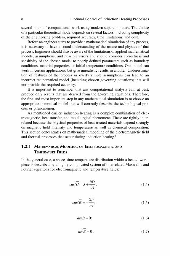
In the general case, a space–time temperature distribution within a heated work-piece is described by a highly complicated system of interrelated Maxwell’s andFourier equations for electromagnetic and temperature fields:
(1.4)
(1.5)
(1.6)
(1.7)
curlH JD= + ∂
∂τ;
curlEB= − ∂
∂τ;
divB = 0 ;
divE = 0 ;
DK6039_C001.fm Page 8 Thursday, June 8, 2006 8:39 AM

Theory and Industrial Application of Induction Heating Processes
9
, (1.8)
where
is a vector of electric field intensity.
is a vector of electric flux density.
is a vector of magnetic flux density.
is a vector of magnetic field intensity.
J
is conduction current density.
t
is temperature.
γ
(
t
) is specific density of the metal.
c(t) is specific heat.λ(t) is thermal conductivity of the metal.
is a vector of velocity.τ is time.
Equation (1.4) to Equation (1.8) includes special notations curl and div. Thesenotations are popular in vector algebra and are used to express particular differ-ential operations. For example, in a rectangular coordinate system, div and curlrepresent the following operations:
; (1.9)
(1.10)
wherei, j, k are unit vectors in the 3 standard Cartesian directions.
The technique of calculating electromagnetic fields depends on the ability tosolve Maxwell’s equations (Equation 1.4 through Equation 1.7) for general time-varying electromagnetic fields.
c t tt
div t grad t c t t Vgrad t( ) ( ) ( ( ) ) ( ) ( )γ ∂∂τ
λ γ− + = −− ⋅div E H[ ]
E
D
B
H
V
divUU
X
U
Y
U
ZX Y Z= ∂
∂+ ∂
∂+ ∂
∂
curlU
i j k
X Y ZU U U
iU
Y
U
Z
X Y Z
Z Y
= ∂∂
∂∂
∂∂
=
= ∂∂
− ∂∂
+ ∂
∂− ∂
∂
+ ∂
∂− ∂
∂
jU
Z
U
Xk
U
X
U
YX Z Y X
DK6039_C001.fm Page 9 Thursday, June 8, 2006 8:39 AM
10 Optimal Control of Induction Heating Processes
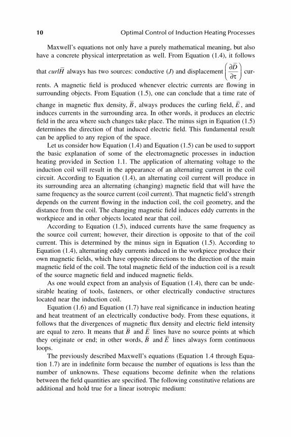
Maxwell’s equations not only have a purely mathematical meaning, but alsohave a concrete physical interpretation as well. From Equation (1.4), it follows
that always has two sources: conductive (J) and displacement cur-
rents. A magnetic field is produced whenever electric currents are flowing insurrounding objects. From Equation (1.5), one can conclude that a time rate of
change in magnetic flux density, , always produces the curling field, , andinduces currents in the surrounding area. In other words, it produces an electricfield in the area where such changes take place. The minus sign in Equation (1.5)determines the direction of that induced electric field. This fundamental resultcan be applied to any region of the space.
Let us consider how Equation (1.4) and Equation (1.5) can be used to supportthe basic explanation of some of the electromagnetic processes in inductionheating provided in Section 1.1. The application of alternating voltage to theinduction coil will result in the appearance of an alternating current in the coilcircuit. According to Equation (1.4), an alternating coil current will produce inits surrounding area an alternating (changing) magnetic field that will have thesame frequency as the source current (coil current). That magnetic field’s strengthdepends on the current flowing in the induction coil, the coil geometry, and thedistance from the coil. The changing magnetic field induces eddy currents in theworkpiece and in other objects located near that coil.
According to Equation (1.5), induced currents have the same frequency asthe source coil current; however, their direction is opposite to that of the coilcurrent. This is determined by the minus sign in Equation (1.5). According toEquation (1.4), alternating eddy currents induced in the workpiece produce theirown magnetic fields, which have opposite directions to the direction of the mainmagnetic field of the coil. The total magnetic field of the induction coil is a resultof the source magnetic field and induced magnetic fields.
As one would expect from an analysis of Equation (1.4), there can be unde-sirable heating of tools, fasteners, or other electrically conductive structureslocated near the induction coil.
Equation (1.6) and Equation (1.7) have real significance in induction heatingand heat treatment of an electrically conductive body. From these equations, itfollows that the divergences of magnetic flux density and electric field intensityare equal to zero. It means that and lines have no source points at whichthey originate or end; in other words, and lines always form continuousloops.
The previously described Maxwell’s equations (Equation 1.4 through Equa-tion 1.7) are in indefinite form because the number of equations is less than thenumber of unknowns. These equations become definite when the relationsbetween the field quantities are specified. The following constitutive relations areadditional and hold true for a linear isotropic medium:
curlH∂∂
D
τ
B E
B EB E
DK6039_C001.fm Page 10 Thursday, June 8, 2006 8:39 AM

Theory and Industrial Application of Induction Heating Processes 11
(1.11)
(1.12)
(1.13)
wherethe parameters ε, µr, and σ denote, respectively, the relative permittivity,
relative magnetic permeability, and electrical conductivity of the material;σ = 1/ρ, where ρ is electrical resistivity.
The constant µ0 is the permeability of free space (the vacuum) and, similarly, theconstant ε0 is the permittivity of free space (see Section 1.1).
By taking Equation (1.11) and Equation (1.13) into account, Equation (1.14)can be rewritten as:
. (1.14)
For most practical applications of the induction heating of metals when thefrequency of current is less than 10 MHz, the induced conduction current density,
J, is much greater than the displacement current density, ; so the last term on
the right-hand side of Equation (1.14) can be neglected. Therefore, Equation(1.14) can be rewritten as:
(1.15)
The Fourier equation (1.8) describes in general the transient (time-dependent)heat transfer process in a metal workpiece. The heating process is caused by heatsources induced by eddy currents (so-called heat generation). The heat sourcedensity, F, induced by eddy currents per unit time in a unit volume can beobtained by solving the electromagnetic problem as:
. (1.16)
The value of specific heat c (in Equation 1.8) indicates the amount of energythat must be absorbed by the workpiece to achieve the required temperaturechange. A high value of specific heat corresponds to a higher required power.
D E= εε0 ;
B Er= µ µ0 ;
J E= σ ;
curlH EE= + ∂
∂σ ε ε
τ( )0
∂∂D
τ
curlH E= σ .
F div E H= − ⋅[ ]
DK6039_C001.fm Page 11 Thursday, June 8, 2006 8:39 AM
12 Optimal Control of Induction Heating Processes
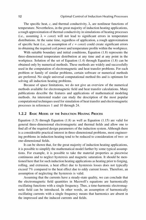
The specific heat, c, and thermal conductivity, λ, are nonlinear functions oftemperature. Nevertheless, in the great majority of induction heating applications,a rough approximation of thermal conductivity in simulations of heating processes(i.e., assuming λ = const) will not lead to significant errors in temperaturedistributions. At the same time, regardless of application, a rough approximationof specific heat (i.e., an assumption of c = const) could create significant errorsin obtaining the required coil power and temperature profile within the workpiece.
With suitable boundary and initial conditions, Equation (1.8) represents thethree-dimensional temperature distribution at any time and at any point in theworkpiece. Solution of the set of Equation (1.4) through Equation (1.8) can beobtained only by numerical methods. These methods are widely and successfullyused in the computation of electromagnetic and heat transfer problems. For eachproblem or family of similar problems, certain software or numerical methodsare preferred. No single universal computational method fits and is optimum forsolving all induction heating problems.
Because of space limitations, we do not give an overview of the numericalmethods available for electromagnetic field and heat transfer calculations. Manypublications describe the features and applications of mathematical modelingmethods. An interested reader can study the description of the most popularcomputational techniques used for simulation of heat transfer and electromagneticprocesses in references 1 and 10 through 24.
1.2.2 BASIC MODEL OF THE INDUCTION HEATING PROCESS
Equation (1.5) through Equation (1.8) as well as Equation (1.15) are valid forgeneral three-dimensional electromagnetic and thermal fields and allow one tofind all of the required design parameters of the induction system. Although thereis a considerable practical interest in three-dimensional problems, most engineer-ing problems in induction heating tend to be reduced to consideration of two- orone-dimensional fields.
It can be shown that, for the great majority of induction heating applications,it is possible to simplify the mathematical model further by some typical assump-tions. For example, it is possible to take the material properties as piecewisecontinuous and to neglect hysteresis and magnetic saturation. It should be men-tioned here that for such induction heating applications as heating prior to forging,rolling, and extrusion, a heat effect due to hysteresis losses does not typicallyexceed 7% compared to the heat effect due to eddy current losses. Therefore, anassumption of neglecting the hysteresis is valid.
Assuming that the currents have a steady-state quality, we can conclude thatthe electromagnetic field quantities in Maxwell’s equations are harmonicallyoscillating functions with a single frequency. Thus, a time-harmonic electromag-netic field can be introduced. In other words, an assumption of harmonicallyoscillating currents with a single frequency means that harmonics are absent inthe impressed and the induced currents and fields.
DK6039_C001.fm Page 12 Thursday, June 8, 2006 8:39 AM

Theory and Industrial Application of Induction Heating Processes 13
For many induction heating applications, the quantities of the magnetic field(such as magnetic vector potential, electric field intensity, and magnetic fieldintensity) may be assumed to be entirely directed. This allows one to reduce thedimensionality of governing equations. Moreover, most mathematical models ofinduction heating tend to be handled with a combination of the following assump-tions:
• Neglecting nonlinearity by averaging process parameters on the cor-responding temperature intervals;
• Mathematical description of heated workpieces as regular bodies(plate, cylinder, rectangle, sphere);
• Simplified description of the geometric input data for induction heatingsystem;
• Taking into account nonuniformity of temperature distribution onlyalong one or two coordinate axes (reducing a three-dimensional tem-perature field to a one- or two-dimensional form).
Under these assumptions, the set of Equation (1.5) through Equation (1.8)and Equation (1.15) can be reduced to the following equations in differential form:
; (1.17)
. (1.18)
Here,∇2 is the Laplacian;x is a spatial coordinate;ω = 2πf, where f is a frequency of coil current;a is average value of temperature conductivity of heated material.
Equation (1.17) is a one-dimensional linear Helmholtz’s equation with respectto complex magnetic field intensity . Equation (1.18) is a one-dimensionallinear heterogeneous equation of heat transfer with respect to temperature t(x,τ)at velocity V = 0. Equation (1.17) and Equation (1.18) can be solved separately.
F(x,τ) is a function described distribution of internal heat source densityinduced by eddy currents per unit time in a unit volume. F(x,τ) can be obtainedby solving Equation (1.17) as:
, (1.19)
∇ =20
H x j H x( , ) ( , )τ ωµ σ τ
∂ τ∂τ
τγ
τt xa t x
cF x
( , )( , ) ( , )= ∇ +2 1
H
F x Em( , )τ σ= 12
2
DK6039_C001.fm Page 13 Thursday, June 8, 2006 8:39 AM
14 Optimal Control of Induction Heating Processes
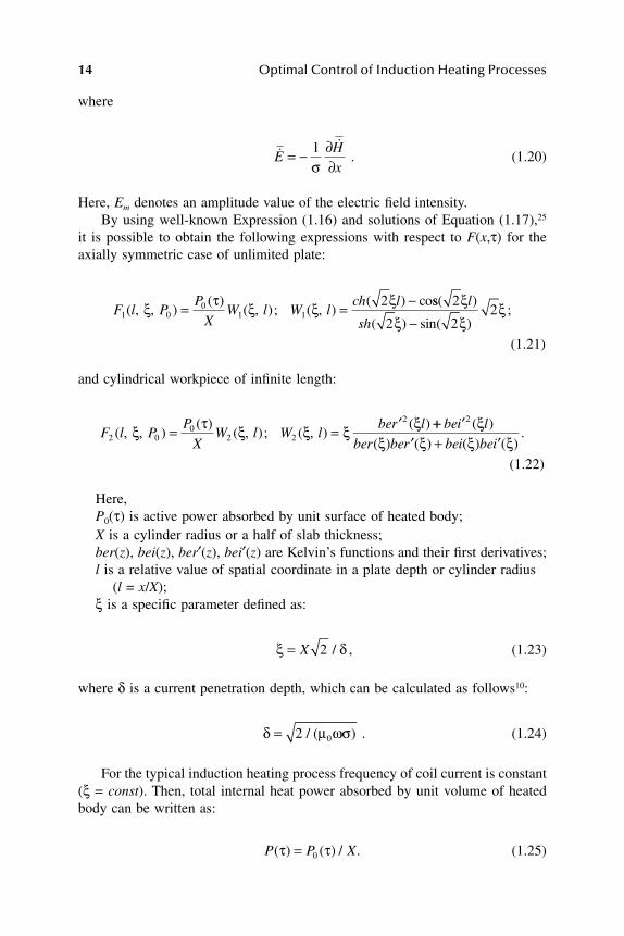
where
. (1.20)
Here, Em denotes an amplitude value of the electric field intensity.By using well-known Expression (1.16) and solutions of Equation (1.17),25
it is possible to obtain the following expressions with respect to F(x,τ) for theaxially symmetric case of unlimited plate:
(1.21)
and cylindrical workpiece of infinite length:
(1.22)
Here,P0(τ) is active power absorbed by unit surface of heated body;X is a cylinder radius or a half of slab thickness;ber(z), bei(z), ber′(z), bei′(z) are Kelvin’s functions and their first derivatives;l is a relative value of spatial coordinate in a plate depth or cylinder radius
(l = x/X);ξ is a specific parameter defined as:
, (1.23)
where δ is a current penetration depth, which can be calculated as follows10:
. (1.24)
For the typical induction heating process frequency of coil current is constant(ξ = const). Then, total internal heat power absorbed by unit volume of heatedbody can be written as:
(1.25)
EH
x= − ∂
∂1σ
F l PP
XW l W l
ch l1 0
01 1
2( , , )
( )( , ); ( , )
( ) coξ τ ξ ξ ξ= = − ss( )
( ) sin( );
2
2 22
ξξ ξ
ξl
sh −
F l PP
XW l W l
ber l2 0
02 2
2
( , , )( )
( , ); ( , )( )ξ τ ξ ξ ξ ξ= = ′ ++ ′′ + ′
bei l
ber ber bei bei
2 ( )( ) ( ) ( ) ( )
.ξ
ξ ξ ξ ξ
ξ δ= X 2 /
δ µ ωσ= 2 0/ ( )
P P X( ) ( ) / .τ τ= 0
DK6039_C001.fm Page 14 Thursday, June 8, 2006 8:39 AM
Theory and Industrial Application of Induction Heating Processes 15
There is a squared relationship between specific power P(τ) and inductorvoltage.10 The value of P(τ) is in the range of 0 to Pmax corresponding to maximuminductor voltage:
. (1.26)
Substituting F(x,τ) in the forms of Equation (1.21) and Equation (1.22) intoEquation (1.18), one can obtain the following one-dimensional linear heteroge-neous equation of heat transfer considered further as a basic mathematical modelof induction heating process:
.
(1.27)
Equation (1.27) is written with respect to relative units of temperature θ(l,ϕ)and power of internal heat sources u(ϕ). These relative values can be calculatedaccording to the formulas:
; (1.28)
. (1.29)
In Equation (1.27),Γ = 0 or Γ = 1 for the plate or cylinder, respectively.W(ξ, l) is determined according to Equation (1.21) or Equation (1.22).
is the Fourier number.
ϕ0 is the total time required for heating.tb is a basic temperature.
The formulation of a problem requiring the solution of a partial differentialequation also requires the specification of appropriate boundary conditions andinitial conditions. Specification of the dependent variable or its time derivativeat time zero is referred to as an initial condition. The initial temperature conditionrefers to the temperature profile within the workpiece at time ϕ = 0:
. (1.30)
0 0≤ ≤ ≥P P( ) ,maxτ τ
∂θ ϕ∂ϕ
∂ θ ϕ∂
∂θ ϕ∂
ξ ϕ( , ) ( , ) ( , )( , ) (
l l
l l
l
lW l u= + +
2
2
Γ)), [ , ]; [ ; ]l ∈ ∈0 1 0 0ϕ ϕ
θ ϕ τ λ( , )( , )
max
lt x t
P Xb= −
2
uP
P( )
( )
max
ϕ τ=
ϕ τ= a
X 2
θ θ( , ) ( )l l0 0=
DK6039_C001.fm Page 15 Thursday, June 8, 2006 8:39 AM
16 Optimal Control of Induction Heating Processes
The initial temperature distribution is usually uniform and corresponds to theambient temperature. In some cases, the initial temperature distribution is non-uniform due to residual heat after the previous technological process. The con-dition in Equation (1.30) is required only when dealing with a transient heattransfer problem where the temperature is a function not only of the spacecoordinates but also of time.
For physical problems, the term “boundary” literally means on the physicalboundary of the region in space in which the solution is sought. The three mostcommon boundary conditions for induction heating problems are:
1. Value of temperature is specified on the boundary of the heated body.This boundary condition is also known as a Dirichlet condition or aboundary condition of the first kind.
2. Normal derivatives of temperature are specified on the boundary. Thiscondition is known as a Neumann condition or a boundary conditionof the second kind.
3. A linear combination of conditions 1 and 2 is specified on the boundary.Convective boundary conditions in heat transfer are of this type. Thiscondition is known as a Robbins condition or a boundary condition ofthe third kind.
If the heated body is geometrically symmetrical along the axis of symmetry,the Neumann boundary conditions can be formulated as:
, (1.31)
. (1.32)
The condition in Equation (1.31) implies that the temperature gradient in adirection normal to the axis of symmetry is zero. In other words, no heat exchangetakes place at the axis of symmetry. This boundary condition can also be appliedin the case of a perfectly insulated body.
In Expression (1.32), q(ϕ) represents a relative value of heat losses and canbe determined as:
. (1.33)
Here, Qs(ϕ) is a flow of heat loss from a surface of the heated body (i.e., duringquenching or as a result of workpiece contact with cold rolls or water-cooledguides, etc.).
∂θ ϕ∂
( , )00
l=
∂θ ϕ∂
ϕ( , )( )
10
lq= <
P Xs( )( )
max
ϕ ϕ=
DK6039_C001.fm Page 16 Thursday, June 8, 2006 8:39 AM
Theory and Industrial Application of Induction Heating Processes 17
For most induction heating problems, boundary conditions include the heatlosses due to convection. In this case, the boundary condition of the third kindcan be expressed as:
, (1.34)
where∂θ/∂l is the temperature gradient in a direction normal to the surface at the
point under consideration.Bi = αX/λ is the Biot number.α is the convection surface heat transfer coefficient.θa(ϕ) denotes a relative value of ambient temperature ta(τ) calculated as:
. (1.35)
The heat losses at the workpiece surface are highly variable because of thenonlinear behavior of convection losses.
Equation (1.27) with boundary conditions in Equation (1.31), Equation (1.32),and Equation (1.34) are the most popular equations for mathematical modelingof the heat transfer processes in induction heating and heat treatment applications.
Let us assume that power of internal heat sources u(ϕ) can be changed almostin an arbitrary way. In this case, the solution of Equation (1.27) under initial andboundary conditions (1.30) through (1.32) and (1.34) can be written in the formof Duhamel integral as25:
. (1.36)
Taking into consideration appropriate boundary conditions of the second (Φ2, Λ2)and the third (Φ3, Λ3) kinds, functions Φ(l, ϕ) and Λ(l, ϕ) can be calculated as25:
; (1.37)
∂θ ϕ∂
θ ϕ θ ϕ( , )( ( ) ( , ))
11
lBi a= −
θ ϕ τ λaa bt t
P X( )
( )
max
= −2
θ ϕ ϕϕ τϕ
τ τϕ
l ll
u d, ,,( ) = ( ) + ∂ −( )∂
( )∫ΦΛ
0
Φ Γ2 00
0
1 2l q dK l
Kn,ϕ θ τ τ
µϕ
( ) = +( ) + ( )
+ ( )∫ 22
1
0
0
2 2
µ
θ µ τµ ϕ
ϕµ ϕ τ
nn
n ne K q en n
( ) ×
× + ( ) ( )
=
∞
− −
∑
∫– (( )
dτ
DK6039_C001.fm Page 17 Thursday, June 8, 2006 8:39 AM

18 Optimal Control of Induction Heating Processes
;
(1.38)
; (1.39)
. (1.40)
In Expression (1.37) through Expression (1.40), the fundamental functions K(µnl),K1(µnl) should be calculated using following expressions:
; (1.41)
(1.42)
where J0(µnl) and J1(µn) are Bessel functions of the zero and first orders, respec-tively.
Under boundary conditions of the third kind, fundamental numbers µn, n =1, 2, … represent roots of the equation:
. (1.43)
Under boundary conditions of the second kind, fundamental numbers µn, n =0, 1, 2, … represent roots of the equation:
. (1.44)
In Expression (1.37) through Expression (1.40):
, n = 0, 1, 2, ….
(1.45)
The finite and sufficient number of terms of series should always be used in givenexpressions.
ΦΓ
3
2
2 2
2
1
2
lBi K l e
Bi Bi K
n nu
n
n
,ϕµ
µ
ϕ
( ) = ( )+ + −( )( )
−
112
1
0 1
0
2
µθ µ µ θ τ τα
ϕ
µ τ
nn
n n nK e dn
( )+ ( ) ( )
=
∞
∑ ∫
Λ Γ2 0 2 21 2l WW K l
Kn n
n nn
,ϕ ξ ϕξ µ
µ µ( ) = +( ) ( ) +
( ) ( )( ) ⋅
==
∞−∑ −
1
12
e nµ ϕ
ΛΓ
3 2 2 22
1l
W K l
Bi Bi K
n n
n n
,ϕξ µ
µ µ( ) = ( ) ( )
+ + −( )( ) ( )nn
e n
=
∞−∑ ⋅ −
1
12µ ϕ
K l l Kn n n n( ) cos ; ( ) sinµ µ µ µΓ Γ= =
= =0
10
K l J l K Jn n n n( ) ( ); ( ) ( ),µ µ µ µΓ Γ= =
= =1
0 11
1
BiK K( ) ( )µ µ µ− =1 0
K1 0( )µ =
W W l l K l dl l l Kn n n nξ ξ µ θ θ µ( ) = ( ) ( ) = ( )∫ ∫0
1
0 0
0
1
, ;Γ Γ ll dl( )
DK6039_C001.fm Page 18 Thursday, June 8, 2006 8:39 AM
Theory and Industrial Application of Induction Heating Processes 19
1.3 TYPICAL INDUSTRIAL APPLICATIONS AND FUNDAMENTAL PRINCIPLES OF INDUCTION MASS HEATING
This book is devoted to a discussion of the use of induction heating principlesfor a large group of applications referred to as mass heating. This term appliesto a variety of applications in which metal is heated for forging, forming, extru-sion, coating, etc. Typically, it is required to have a uniformly heated workpiece.However, it is sometimes necessary to heat certain areas of the workpiece selec-tively and care must be taken to provide a required temperature distribution.
Temperature greatly affects the formability of metals. Heating of a componentto temperatures that correspond to the plastic deformation range creates a favor-able condition for metal to be subsequently forced by various means into a desiredshape. The most popular metal hot working processes for which induction heatingis applied follow.1
• Forging. Billets or bars are heated fully or partially, in cut length orcontinuously, and are forged in presses, hammers (repeated blows), orupsetters (which gather and form the metal). Steel components by farrepresent the majority of forged parts. At the same time, aluminum,copper, brass, bronze, cobalt, nickel, and titanium, as well as someother metal alloys, are also inductively heated and forged for a numberof commercial applications.
• Forming. Hot forming includes a variety of metal working operationsgenerally encompassing bending, expanding, and spinning. The versa-tility of induction heating is that it can selectively heat through specificareas of the workpiece or can heat areas to different temperaturesproviding required temperature gradients, making it a popular choicefor hot forming operations.
• Extrusion. Extruding is the process of forcing or squeezing metalthrough a die. Ferrous and nonferrous metals are heated by inductionprior to extrusion.
• Rolling. Bars, billets, rods, slabs, blooms, strips, and sheets are pro-cessed in rolling mills. These components are made from ingots orcontinuous cast metals and their alloys.
The goal of using induction heating in all of these applications is to providethe metal workpiece at the hot working stage with the desired (typically uniform)temperature across its diameter/thickness as well as along its length and acrossits width. The required final temperature typically depends on the material chem-ical composition and particularities of the postheating metal processing operation.For example, for steel billets, the final temperature is in the range of 1000 to1200°C and the required surface-to-core and noise-to-tail temperature uniformityin the billet is commonly specified as ±50°C for rolling and ±25°C for forming.For heating of aluminum alloy billets before extrusion, the final temperature is
DK6039_C001.fm Page 19 Thursday, June 8, 2006 8:39 AM

20 Optimal Control of Induction Heating Processes
in the range of 450 to 480°C and required uniformity is in the range of ±10 to±15°C. Certain applications may require a nonuniform end-to-end temperatureprofile (for example, heating providing required temperature gradients).
In some cases, the initial temperature of the workpiece prior to inductionheating is the ambient temperature. In other cases, the initial temperature is notuniform — for example, due to uneven cooling of the slab, transfer bar, strip, orbloom as it progresses from the caster. Surface layers, and particularly the edgeareas, become much cooler than the internal regions.
The power ratings of induction heating machines range from less than 100kW up to dozens of megawatts. The success of an induction mass heating systemis based on an in-depth understanding of the process features. This is imperativefor developing the sophisticated design concepts and precise engineering thatlead to the achievement of a reasonable, commercially acceptable compromiseamong often contradictory process requirements and design criteria.
Cylindrical and rectangular solenoid multiturn induction coils are most oftenused in induction mass heating applications. The four basic heating modes ininduction mass heating (Figure 1.4) follow.1
• Static heating. In the static heating mode, a workpiece such as a billetor slab is placed into an induction heating coil for a given period oftime while a set amount of power is applied until the componentreaches the desired heating conditions. Upon reaching the required
FIGURE 1.4 Four basic heating modes used in induction mass heating.
Multi-turn solenoid
induction coil
Heated workpiece
(a) Static heating
Coil #1
Heated workpiece
Heated workpiece
(c) Oscillating heating
(b) Progressive multi-stage heating and continous heating
Coil #2 Coil #3
Coil #1 Coil #2 Coil #3
Refractory
DK6039_C001.fm Page 20 Thursday, June 8, 2006 8:39 AM

Theory and Industrial Application of Induction Heating Processes 21
thermal conditions, the heated component is extracted from the induc-tion heater and delivered to the metal forming station. The next coldworkpiece is loaded into the coil and the process repeats.
• Progressive multistage heating. This heating mode occurs when twoor more heated workpieces (e.g., billets) are moved (via pusher, index-ing mechanism, walking beam, etc.) through a single-coil or multicoilinduction heater. Therefore, components are sequentially heated (in aprogressive manner) at certain predetermined heating stages inside theheater.
• Continuous heating. With the continuous heating mode, the workpieceis moved in a continuous motion through one or more induction heatingcoils. This heating mode is commonly used when it is required to heatlong components such as bars, slabs, strips, tubes, wires, blooms, androds.
• Oscillating heating. In this heating mode, a component moves backand forth (oscillates) during the process of heating inside a single-coilor multicoil induction heater with an oscillating stroke featuring aspace-saving design approach.
When modern induction mass heating systems are designed, temperatureuniformity of the heated component is only one of the goals. Additional designcriteria include maximum production rate, minimum metal losses, and the abilityto provide flexible and compact systems that have high electrical efficiency. Otherimportant factors include quality assurance, process repeatability, automationcapability, environmental friendless, reliability, and maintainability of the equip-ment. The last criterion, but not the least, is the competitive cost of an inductionheating system.
One of the challenges in induction heating arises from the necessity to providethe required surface-to-core temperature uniformity. Due to the physics of theprocess, the workpiece core tends to be heated more slowly than its surface. Themain reason for the heat deficit of the heated component is the skin effectdiscussed earlier.
It has been pointed out that, in induction heating, the heat transfer by con-vection and radiation reflects the value of surface heat losses. This heat loss varieswith temperature. The analysis shows that the convection losses are the majorpart of the heat loss in low-temperature applications such as induction heatingof tin, lead, and aluminum alloys. In hot working applications (including inductionheating of steel, titanium, cobalt, and nickel), radiation losses are much greaterthan convection losses, representing the major portion of total heat loss from theworkpiece surface.
It is typically much easier to provide surface-to-core temperature uniformityfor metals with high thermal conductivity, such as aluminum, silver, or copper.Metals with poor thermal conductivity, including stainless steel, titanium, andcarbon steel, require extra care to obtain the desired temperature uniformity. This
DK6039_C001.fm Page 21 Thursday, June 8, 2006 8:39 AM
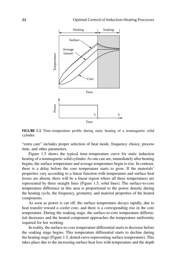
22 Optimal Control of Induction Heating Processes
“extra care” includes proper selection of heat mode, frequency choice, processtime, and other parameters.
Figure 1.5 shows the typical time–temperature curve for static inductionheating of a nonmagnetic solid cylinder. As one can see, immediately after heatingbegins, the surface temperature and average temperature begin to rise. In contrast,there is a delay before the core temperature starts to grow. If the materials’properties vary according to a linear function with temperature and surface heatlosses are absent, there will be a linear region where all three temperatures arerepresented by three straight lines (Figure 1.5, solid lines). The surface-to-coretemperature difference in this area is proportional to the power density duringthe heating cycle, the frequency, geometry, and material properties of the heatedcomponents.
As soon as power is cut off, the surface temperature decays rapidly, due toheat transfer toward a cooler core, and there is a corresponding rise in the coretemperature. During the soaking stage, the surface-to-core temperature differen-tial decreases and the heated component approaches the temperature uniformityrequired for hot working.
In reality, the surface-to-core temperature differential starts to decrease beforethe soaking stage begins. This temperature differential starts to decline duringthe heating stage (Figure 1.5, dotted curve representing surface temperature). Thistakes place due to the increasing surface heat loss with temperature and the depth
FIGURE 1.5 Time–temperature profile during static heating of a nonmagnetic solidcylinder.
Heating
Surface
Average
(mean)
Core
Time
Time
tft1
Tem
per
atu
reP
ow
er
Soaking
DK6039_C001.fm Page 22 Thursday, June 8, 2006 8:39 AM

Theory and Industrial Application of Induction Heating Processes 23
of induction heating during the heating cycle. Because the electrical resistivityof most metals increases with temperature, current penetration depth increases.
It is important to note that the soaking stage can be performed when theheated workpiece is inside the induction coil and/or during the workpiece transferstage to the hot forming machinery. The latter approach allows minimizing thetotal process time.
It should be mentioned that, in reality, the time–temperature profiles are morecumbersome than those shown in Figure 1.5. To improve the performance of aninduction heating machine and reduce the heating time while providing surface-to-core temperature uniformity, power pulsing can be applied. Power pulsingrefers to a technique that applies short bursts of power to maintain a desiredsurface temperature or a maximum allowable surface-to-core temperature differ-ence. Pulse heating consists of a series of “Heat ON” and “Heat OFF” cyclesuntil the desired uniformity is obtained (Figure 1.6). Depending upon the partic-ular application, the process time reduction with pulse heating can exceed 40%.
The heating time can be reduced even more when applying acceleratedheating (Figure 1.7). Obviously, to provide this type of heating, it is necessaryto have a power supply that allows a gradual reduction of output power. Theaccelerated heating approach may have several modifications. Figure 1.8 shows
FIGURE 1.6 Power pulsing.
Surface
Average
(mean)Core
Time
Time
tft1 t2 t3
Tem
per
atu
re
Tmax
Maximum permissible
temperature
Required
temperature
Tfinal
Po
wer
Time
reduction
compared to
single
heating time
DK6039_C001.fm Page 23 Thursday, June 8, 2006 8:39 AM

24 Optimal Control of Induction Heating Processes
FIGURE 1.7 Accelerated heating.
FIGURE 1.8 Modification of accelerated heating.
Surface
Average
(mean)
Core
Time
Time
tft1 t2
Tem
per
atu
re
Tmax
Maximum permissible
temperature
Required
temperature
Tfinal
Po
wer
Surface
Avoidance of
exceeding the
critical values of
thermal gradients
Core
Time
Time
Tem
per
atu
re
Tmax
Tfinal
Po
wer
DK6039_C001.fm Page 24 Thursday, June 8, 2006 8:39 AM

Theory and Industrial Application of Induction Heating Processes 25
one of the modifications of accelerated heating that is particularly useful whenheated bars, slabs, or billets have a tendency to crack. These cracks appear dueto excessive thermal stresses (thermal shocks) that appear when thermal gradientsexceed the maximum permissible level. These levels vary depending upon themetal’s chemical composition, microstructure, and temperature.
Although it has been mentioned that the curves shown in Figure 1.5 throughFigure 1.8 illustrate typical time–temperature profiles that take place during staticheating, these curves are practically identical for progressive multistage heatingand continuous heating modes as well. For multistage or continuous heating, thetime axis represents the length of the induction heating line or coil length. Burstsof power can represent the power of inline coils that may have different lengthand windings, and/or can be individually fed from different power supplies withthe ability to adjust the output power and frequency.1
1.4 DESIGN APPROACHES OF INDUCTION MASS HEATING
There are many different types of induction heating coils. The ability of any coilto establish a magnetic field depends upon the ampere-turns of the coil, geometry,and its electrical circuit. The selection of power, frequency, and coil length ininduction heating is highly subjective, depending upon the type of heated metal,required temperature uniformity, time of heating, and so on. Frequency is one ofthe most critical parameters in these applications. If the frequency is too low, aneddy current cancellation within the heated body will take place, resulting in poorcoil efficiency.
However, when the frequency is too high, the skin effect will be highlypronounced, resulting in a current concentration in a very thin surface layercompared to the diameter/thickness of the heated component. In this case, alengthy heating time will be required to provide sufficient heating of the internalareas and the core. Prolonged heat time results in an increase of the radiation andconvection heat losses that, in turn, reduce the thermal efficiency of the inductionheater and diminish the main advantage of induction heating. Frequency is alwaysa reasonable compromise.
The determination of the length of the coil line is another important step inspecifying an induction heating system. In determining how long the coil lineneeds to be, the time required for heating the workpiece to an acceptable tem-perature condition is actually being determined. Heating time is a complex func-tion of various factors, including the size of the workpiece, frequency, heatingmode, power density, maximum permissible temperature, material properties, andthe required surface-to-core temperature uniformity.
Coil design is, of course, an extremely important factor in developing anefficient induction heating system. Solenoid type (helical) multiturn coils are mostoften used in induction heating applications. The electrical efficiency and coilcoupling have a marked effect on the coil’s ability to deliver heating power to
DK6039_C001.fm Page 25 Thursday, June 8, 2006 8:39 AM

26 Optimal Control of Induction Heating Processes
the workpiece. Smaller gaps between the surface of the heated workpiece andthe coil result in better electromagnetic coupling and, consequently, higher coilefficiency. However, it is wise to remember that the total efficiency of the induc-tion coil is a product of coil electrical efficiency and coil thermal efficiency.
Nearly all induction coils used for heating prior to hot forming of metalsconsist of thermal isolation (also called refractory or liners) between the coil andthe heated workpiece protecting the coil windings from heat exposure and pro-viding a thermal barrier. Thus, the chance of thermal shock is reduced and heatloss is minimized in water recirculating through the induction coil.
The thermal refractory can drastically decrease the heat losses from thesurface of the heated workpiece. At the same time, the use of a refractorynecessitates larger coil-to-workpiece gaps, which in turn deteriorates the electro-magnetic coupling between the induction coil and the heated workpiece, leadingto a reduction of coil electrical efficiency (Figure 1.9). Thus, the refractory allowsone to improve coil thermal efficiency, but it also reduces coil electrical efficiency.In the great majority of mass heating applications and, in particular, in heatingprior to hot working, it is advantageous to use refractory. Its minimum thicknessis usually about 12 mm (0.5 in.). Different materials can be used for manufac-turing refractory. These include castable (i.e., Visil), silicon carbide, Alumina, H-91, Zircar, and other fibrous ceramic materials.
The two principal approaches to building coils can be categorized as the open-wound or the refractory-encased approach. The open-wound method providesmore convenient repair in the event of failure but the choice is never that simple.Replaceable refractory liners are commonly utilized in the construction of open-wound coils. Coils with replaceable liners have lower repair time and cost com-pared to cast coils.
FIGURE 1.9 Coil electrical and thermal efficiencies vs. thickness of refractory.
Thickness of refractory
Electrical efficiency
Thermal efficiency
Co
il e
ffici
enc
y
DK6039_C001.fm Page 26 Thursday, June 8, 2006 8:39 AM

Theory and Industrial Application of Induction Heating Processes 27
Although the encased coil using a castable refractory offers durability andlonger life, it still follows recommended maintenance routines that should not beneglected. To repair a cast coil, it must be shipped to a service center where it isbroken down to the bare coil. Then the coil must be repaired, reinsulated, andrecast. This process is time consuming considering that the operator can replacerefractory liners on site in a matter of minutes.
Self-supporting internal water-cooled skid rails to protect linear surfaces mustbe robust enough to carry the full load of heated billets with minimal deflection;however, from another perspective, they should be transparent enough to theelectromagnetic field that they will not be significantly heated. Water-cooled railsoccupy space inside the coil and consume additional coolant, thus increasing thekilowatt losses. These rails terminate beyond the open-wound coil box envelopeand extra expansion of longer rails must be accommodated.
To extend the life of water-cooled rails, they are wear coated. In the past,stellite was applied to the surface of the rails as a wear coating. This required anapplication process that works by fusing this material to the surface of the railby heating with an oxygen acetylene torch. By replacing this with a less labor-intensive plasma coating process, it is possible to apply a wider variety of mate-rials, including tungsten carbide and chrome carbide, providing longer rail life.
In addition to water-cooled alloy skid rails, various ceramic materials havebeen developed for use as wear plates. Ceramic liners are embedded into therefractory surface and have been successful in many applications. For high-wear/high-temperature applications, the liners are manufactured from specialalloys.
In addition to improved alloys, new tubing may be provided with an extraheavy wall section that affords a much thicker wear area comparable to weldingan additional layer of material to the top side of the water-cooled rail. These railsalso utilize a plasma-applied wear coating on the surface to afford additionalwear resistance and longer life.
In applications in which refractory liners are made from materials withextremely high wear-resistant properties, some end users actually skid or conveythe billets across the surface of the ceramic liner, thus eliminating the use of skidrails and any cold spots resulting from their use.
Most manufactured liners are round. For cylindrical billets, a round shapedliner naturally suits the coil geometry. However, when heating square billets, thismismatch of shapes may result in a noticeable increase of the coil opening inaddition to space allowances for the skid rails and thermal insulation. This reducesthe electromagnetic coupling between the coil and billet. Longer coils call for alarger thickness of the refractory to ensure mechanical strength.
To optimize the design, the manufacturers of induction heating systems havedeveloped different procedures. For example, Newelco windings are plasticcoated for insulation purposes before they are set in a high-quality refractorycement. After the winding is positioned in a carefully prepared and assembledbox, a former is centrally inserted through it to create the coil tunnel. Therefractory is poured around the winding in such manner that air pockets are
DK6039_C001.fm Page 27 Thursday, June 8, 2006 8:39 AM
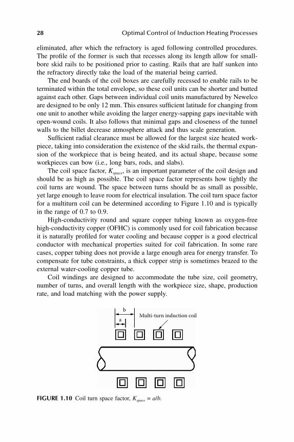
28 Optimal Control of Induction Heating Processes
eliminated, after which the refractory is aged following controlled procedures.The profile of the former is such that recesses along its length allow for small-bore skid rails to be positioned prior to casting. Rails that are half sunken intothe refractory directly take the load of the material being carried.
The end boards of the coil boxes are carefully recessed to enable rails to beterminated within the total envelope, so these coil units can be shorter and buttedagainst each other. Gaps between individual coil units manufactured by Newelcoare designed to be only 12 mm. This ensures sufficient latitude for changing fromone unit to another while avoiding the larger energy-sapping gaps inevitable withopen-wound coils. It also follows that minimal gaps and closeness of the tunnelwalls to the billet decrease atmosphere attack and thus scale generation.
Sufficient radial clearance must be allowed for the largest size heated work-piece, taking into consideration the existence of the skid rails, the thermal expan-sion of the workpiece that is being heated, and its actual shape, because someworkpieces can bow (i.e., long bars, rods, and slabs).
The coil space factor, Kspace, is an important parameter of the coil design andshould be as high as possible. The coil space factor represents how tightly thecoil turns are wound. The space between turns should be as small as possible,yet large enough to leave room for electrical insulation. The coil turn space factorfor a multiturn coil can be determined according to Figure 1.10 and is typicallyin the range of 0.7 to 0.9.
High-conductivity round and square copper tubing known as oxygen-freehigh-conductivity copper (OFHC) is commonly used for coil fabrication becauseit is naturally profiled for water cooling and because copper is a good electricalconductor with mechanical properties suited for coil fabrication. In some rarecases, copper tubing does not provide a large enough area for energy transfer. Tocompensate for tube constraints, a thick copper strip is sometimes brazed to theexternal water-cooling copper tube.
Coil windings are designed to accommodate the tube size, coil geometry,number of turns, and overall length with the workpiece size, shape, productionrate, and load matching with the power supply.
FIGURE 1.10 Coil turn space factor, Kspace = a/b.
bMulti-turn induction coil
a
DK6039_C001.fm Page 28 Thursday, June 8, 2006 8:39 AM
Theory and Industrial Application of Induction Heating Processes 29
Coil cooling is a very important aspect of a heater design. It is obvious thatcoil cooling should be as close as possible to the heating face. Tube wall thicknessis chosen based on the system operating frequency. The heating face wall thick-ness should increase as the frequency decreases. For example, a system with lowoperating frequency requires a thicker wall tube than a high-frequency system.This fact is directly related to the current penetration depth in the copper (δ1) andholds true for tubing coils and coils made from copper sheet. The coil electricallosses will be minimum if the copper tubing wall thickness is greater than 1.6δ1.A coil tubing wall smaller than 1.6δ1 results in a reduction in coil efficiency andan increase of coil tubing power losses.
In some cases, the tubing wall may be thicker than that calculated accordingto the previously mentioned recommendation. This is because it may not bemechanically reliable to use wall tubing that is too thin due to the mechanicalflexing caused by electromagnetic forces. As the frequency is lowered, moreattention must be paid to coil support because there is more vibration at lowerfrequencies, especially at the turns near both ends of multiturn solenoid coils.
High-dielectric epoxies and some nylons are often used as dielectric insulatingmaterials that eliminate arcing between coil windings. A fluidized bed processor an electrostatic coating process can provide dielectric insulation. In certaincases, some ceramic coatings afford protections from high-temperature exposureand suitable dielectric stress.1
1.5 TECHNOLOGICAL COMPLEX “HEATER–EQUIPMENT FOR METAL HOT WORKING”
The principal distinctive feature of the system approach is a necessity to take intoconsideration the whole sequence of the interconnected technological processes(preheating, transfer, hot working) as a technological complex being controlled.Overall performance indexes can be considered when optimizing technologicalcomplex heater–hot working equipment as a whole.
For a particular technological complex, it is important to reveal, by meansof valid decomposition, local cost functions for each stage of the technologicalprocess. Along with these criteria, it is possible to find proper optimal controlinputs, to determine optimal parameters for considered technologies, and to setoptimal initial data values for design solutions. Such an optimization approachoffers some advantages in comparison with typical approaches that simply relyon independent control of the individual processes.
Obtained results lead control algorithms’ abilities out beyond the frameworkof traditional tasks of “serving to” technology, thus ensuring their active partici-pation in its formation. This objective is fulfilled first by means of incidentalsolution of principal development problems for optimal technological modes and,second, by optimal design of production equipment from the point of view of itsfurther optimal operating.
DK6039_C001.fm Page 29 Thursday, June 8, 2006 8:39 AM
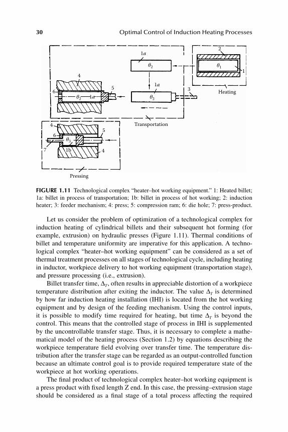
30 Optimal Control of Induction Heating Processes
Let us consider the problem of optimization of a technological complex forinduction heating of cylindrical billets and their subsequent hot forming (forexample, extrusion) on hydraulic presses (Figure 1.11). Thermal conditions ofbillet and temperature uniformity are imperative for this application. A techno-logical complex “heater–hot working equipment” can be considered as a set ofthermal treatment processes on all stages of technological cycle, including heatingin inductor, workpiece delivery to hot working equipment (transportation stage),and pressure processing (i.e., extrusion).
Billet transfer time, ∆T, often results in appreciable distortion of a workpiecetemperature distribution after exiting the inductor. The value ∆T is determinedby how far induction heating installation (IHI) is located from the hot workingequipment and by design of the feeding mechanism. Using the control inputs,it is possible to modify time required for heating, but time ∆T is beyond thecontrol. This means that the controlled stage of process in IHI is supplementedby the uncontrollable transfer stage. Thus, it is necessary to complete a mathe-matical model of the heating process (Section 1.2) by equations describing theworkpiece temperature field evolving over transfer time. The temperature dis-tribution after the transfer stage can be regarded as an output-controlled functionbecause an ultimate control goal is to provide required temperature state of theworkpiece at hot working operations.
The final product of technological complex heater–hot working equipment isa press product with fixed length Z end. In this case, the pressing–extrusion stageshould be considered as a final stage of a total process affecting the required
FIGURE 1.11 Technological complex “heater–hot working equipment.” 1: Heated billet;1a: billet in process of transportation; 1b: billet in process of hot working; 2: inductionheater; 3: feeder mechanism; 4: press; 5: compression ram; 6: die hole; 7: press-product.
4
5
5
4
Pressing
θ2
θ3
θ2
θ2 θ1
1a
1b
1a 3
2
1
Heating
Transportation
1a
6
6
7
4
DK6039_C001.fm Page 30 Thursday, June 8, 2006 8:39 AM

Theory and Industrial Application of Induction Heating Processes 31
billet temperature state. An appropriate mathematical model is needed to describehow the temperature field is changed over the stage of processing by pressure.
Hot working operation imposes the two most general requirements on thetemperature field. First, maximum value, θmax(ϕ), of the temperature within theheated workpiece volume is restricted by the certain limiting value, θadm . Second,the temperature differences within the heated workpiece should be restrictedduring the heating process so that the maximum value, σmax, of expanding thermalstresses σ(l, ϕ) (that appeared due to temperature differences) would not exceedprescribed admissible value σadm that corresponds to ultimate stress limit of theheated material. Temperature within the heated workpiece during pressing isrestricted by maximum admissible temperature in the die hole, θcr .
Heating power, F*(t), and pressing velocity, Vp, can be considered as controlinputs for heating and pressing processes. The values of these control inputs arealso restricted by certain limiting admissible values, F*
max and Vpmax.Under previously described conditions, the statement of an optimal control
problem can be formulated for technological complex heater–hot working equip-ment as follows. It is required to get a final press product of desired length andhold cost criteria at extremum value by time-varying controls that is restrictedby a preassigned set and that satisfies the constraints on a temperature distribution.
When maximum productivity is required, a minimal total heating time, τend,can be considered as a cost criterion. When a criterion of minimum cost isrequired, then, depending upon the situation, different performance indexes couldbe considered. Particular OCP formulations for the technological complex andmethods to determine optimal control inputs will be discussed in Chapter 6 ofthe book.
1.6 TECHNOLOGICAL AND ECONOMIC ADVANTAGES OF INDUCTION HEATING
Induction heating installations are of considerable current use in industry. In thepast three decades, heating by induction has become more popular. A major reasonis the ability to create high heat intensity very quickly at well-defined locationson the part. This leads to low process cycle time (high production rate) withrepeatable quality. Induction heaters offer several advantages over analogueequipment.
Induction heating is particularly useful when highly repetitive operations areperformed. Once an induction heating machine is properly adjusted, part afterpart is heated with identical results. Usually, no further attention is required,except the loading and unloading of the workpieces. The ability of inductionheating to heat successive parts identically means that the process is adaptableto completely automatic operation, in which the workpieces are loaded andunloaded mechanically with no operator present.
Induction heating can be utilized in line with other technological operations.This saves the time of transporting heated workpieces from one part of the factory
DK6039_C001.fm Page 31 Thursday, June 8, 2006 8:39 AM
32 Optimal Control of Induction Heating Processes
to another. Another attractive characteristic of induction heating is its ability toheat only a certain part of a workpiece if required.
Induction heating is more energy efficient and inherently more environmen-tally friendly than most other heat sources, including gas-fired furnaces, salt andlead baths, carburizing, or nitriding systems.26–28 Any smoke and fumes that mayoccur due to residual lubricants or other surface contaminants can be easilyremoved. A considerable reduction of heat exposure is another factor that con-tributes to the environmental friendliness of induction heaters.
Induction heating provides much better surface quality of heated metal incomparison with competitive technologies. A significant reduction of scale resultsin substantial metal savings.
Induction systems usually require far less startup and shutdown time andlower labor cost for machine operators. Other important factors of inductionheating machinery include quality assurance, automation capability, high reliabil-ity, and easy maintainability of the equipment. In many cases, induction heatingwill require minimum shop floor space and produce less distortion in the work-piece.
In the past, fuel-fired furnaces that utilized natural gas, fuel oil, or liquidpetroleum gases were often used because of the low cost of fuel. However, inrecent decades, producers have been shifting their preference toward inductionheating systems and this tendency continues to grow at an increasing pace. Thereare several reasons for this shift.
First, fuel-fired furnaces demand a very long heating tunnel to achieve thedesired temperature uniformity. The large required space often presents a problemin plants due to the limited space available on the shop floor, particularly whenthe heating systems must be incorporated into an already existing production line.For example, it is frequently necessary to locate a slab or transfer a bar edgereheater into the limited space between an existing caster and rolling mill.
On the other hand, heating in fuel-fired furnaces results in a significant metalloss and poor surface quality (due to scale formation, decarburization, oxidation,coarse grains, etc.). Scale reduction and improved surface quality of heated partslead to longer die life and minimum postprocessing operations. Unlike fuelheating in which heat is transferred by radiation, the induction-type energy trans-fer generates the heat directly in the workpiece.
Finally, fuel-fired heating increasingly faces environmental restrictions (airpollution) and restrictions from an ergonomic perspective because operators areexposed to hot air blasts and unstable work flow.
These are only some factors that have resulted in induction heating becominga more popular approach for thorough heating of slabs, blooms, billets, bars,tubes, strips, wires, rods, and other components made of ferrous and nonferrousmetals.1
DK6039_C001.fm Page 32 Thursday, June 8, 2006 8:39 AM
Theory and Industrial Application of Induction Heating Processes 33
REFERENCES
1. Rudnev, V.I. et al., Handbook of Induction Heating, Marcel Dekker, New York,2003.
2. Gebhart, B., Heat Transfer, 2nd ed., McGraw–Hill, New York, 1971.3. Patankar, S., Numerical Heat Transfer and Fluid Flow, Hemisphere, New York,
1980.4. Incropera, E.P. and Dewitt, D.P., Fundamentals of Heat Transfer, Wiley, New York,
1981.5. Myers, R.F., Conduction Heat Transfer, McGraw–Hill, New York, 1972.6. Rohsenow, W.M. and Hartnett, J.P., Handbook of Heat Transfer, McGraw–Hill,
New York, 1973.7. Siegel, R.I. and Howell, J.R., Thermal Radiation Heat Transfer, 2nd ed.,
McGraw–Hill, New York, 1980.8. Wiebelt, J.A. and Howell, J.R., Engineering Radiation Heat Transfer, Holt, Rine-
hart & Winston, New York, 1980.9. Leslie, W.C., The Physical Metallurgy of Steels, McGraw–Hill, New York, 1981.
10. Sluhotskii, A.E., Nemkov, V.S., and Pavlov, N.A., Induction Heating Installations,Energoatomizdat, St. Petersburg, 1981.
11. Nemkov, V.S., Polevodov, B.S., and Gurevich, S.G., Mathematical Modeling ofHigh Frequency Heating Equipment, Energoatomizdat, St. Petersburg, 1991.
12. Sluhotskii, A.E. et al., Induction Heating Equipment, Energoatomizdat, St. Peters-burg, 1981.
13. Nemkov, V.S. and Demidovich, V.B., Theory and Computation of Induction Heat-ing Installations, Energoatomizdat, St. Petersburg, 1988.
14. Rudnev, V.I., Mathematical simulation and optimal control of induction heatingof large-dimensional cylinders and slabs, Ph.D. thesis, Electrical EngineeringUniversity, St. Petersburg, 1986.
15. Samarskii, A.A., Theory of Finite Difference Schemes, Nauka, Moscow, 1977.16. Demirchian, K.S. and Chechurin, V.L., Computational Methods of Electromag-
netic Field Simulations, MEI, Moscow, 1986.17. Muehlbauer, A., Software for modeling induction heating equipment by using
finite element method, Appl. Therm. Eng., 23, 1647, 1991.18. Boergerding, R. and Muehlbauer, A., Numerical calculation of temperature dis-
tribution and scale formation in induction heaters for forging, Proc. UIE Sem.“Simulation and Identification of Electroheat Processes,” 134, 1997.
19. Muehlbauer, A., Aktuelle Forschungsbeiträge zur EMV — Magnetische Streufelderin der Umgebung von Induktionsanlagen, EMC Kompendium, Muenchen, 1999.
20. Jin, J.M., The Finite Element Method in Electromagnetics, Willey, New York,1993.
21. Lowther, D.A. and Silvester, P.P., Computer-Aided Design in Magnetics, Springer,Berlin, 1986.
22. Livesley, R.K., Finite Elements: an Introduction for Engineers, Cambridge Uni-versity Press, New York, 1983.
23. Tamm, I.E., Fundamentals of the Theory of Electricity, Moscow, Metallurgy, 1981.24. Hayt, W.H., Engineering Electromagnetics, McGraw–Hill, New York, 1981.25. Rapoport, E.Ya., Optimization of Induction Heating of Metals, Metallurgy,
Moscow, 1993.
DK6039_C001.fm Page 33 Thursday, June 8, 2006 8:39 AM

34 Optimal Control of Induction Heating Processes
26. Muehlbauer, A., Industrielle Elektrowärmetechnik, Vulkan Verlag, Essen, 1992. 27. Baake, E., Joern, K.-U., and Muehlbauer, A., Energiebedarf und CO2-Emission
Industrieller Prozessverfahren, Vulkan–Verlag, Essen, 1996.28. Tudbury, C.A., Basics of Induction Heating, Rider, New York, 1960.
DK6039_C001.fm Page 34 Thursday, June 8, 2006 8:39 AM
35
2
Optimization Problems for Induction Heating Processes
This chapter provides a detailed conceptual description of the optimization prob-lems for induction heating processes (IHPs) prior to metal hot working operations.The optimization problems are discussed from the standpoint of the moderntheory of optimal control with respect to systems with distributed parameters. Aninduction heating process can be considered an example of a system under control.The typical cost functions and mathematical models are provided in this chapter.Some explanations will be given to facilitate understanding such terms as con-trolled outputs and control inputs, disturbances, constraints, etc.
An overview of the most typical and important process constraints takingplace in induction heating will be provided in this chapter as well. Consideredconstraints include but are not limited to power supply limitations, technologicalrequirements, and specifics of the heater design. Requirements to final tempera-ture distribution within a billet will also be discussed in this chapter. The opti-mization problem with respect to IHP simplified models will be formulated interms typically used in the theory of applied optimal control.
The accurate and approximated approaches are presented here to transformthe complicated optimal control problem into a much simpler task of determiningunknown parameters of sought control functions. These parameters make clearphysical sense and define controls uniquely. This procedure is called parameter-ization. A highly effective special engineering parameterization technique hasbeen developed and will be demonstrated. As an example, this unique techniquewill be illustrated by solving a typical optimization problem for an IHP that willallow maximizing production rate of the heating system.
2.1 OVERVIEW OF INDUCTION HEATING PRIOR TO METAL HOT WORKING OPERATIONS AS A PROCESS UNDER CONTROL
The main purpose of induction heating installations (IHIs) is to provide a requiredworkpiece temperature state prior to further stages of the technological process(i.e., hot forming, forging, rolling, extrusion, etc.). An IHI should provide a metalworkpiece (i.e., billet, slab, or bar) at the hot working stage with the desired
DK6039_C002.fm Page 35 Friday, June 9, 2006 7:46 AM
© 2007 by Taylor & Francis Group, LLC

36
Optimal Control of Induction Heating Processes
(typically uniform) temperature distribution across its diameter/thickness as wellas along its length and across its width.
There are several ways to estimate a tolerable deviation of final temperaturedistribution from a desired one. It is typically necessary to provide the fixedmaximum absolute value of temperature variation. This means that at the end ofthe heating the temperature in any point of the billet should deviate not morethan by prescribed value
ε
from desired temperature
θ
*
(Figure 2.1). Anotherapproach might deal with an estimation of the root mean square error betweenthe required temperature distribution and the actual final temperature distribution.
Certain applications may require a nonuniform end-to-end temperature profile(for example, heating providing required temperature gradients). However, thevariation of final temperature distribution from desired one has the same meaningas in the case of uniform heating and could be estimated in the same manner.Thus, the ultimate goal of the heating process prior to consequent hot workingoperation is to obtain a desired temperature profile within a workpiece that wouldcorrespond to particular heating requirements.
In such a case, the induction heating process can be considered as a dynamiccontrolled system, evolving over time. An ability to control the heating processmeans a capability to influence a temperature field in order to achieve a desiredgoal. Therefore, temperature distribution can be defined as
an output controlledfunction
of the process. It is important to recognize that a temperature field varieswith time and spatial coordinates (within workpiece volume). Temperature dis-tribution can be affected through a set of
control inputs
(or
controls
). By choosingin every instant the value of each control input, one can modify temperaturedistribution and dynamic behavior of an induction heating system.
As the ultimate goal, required final temperature distribution could be achievedby different means, including different operating modes of heating systems, coildesign specifics, etc. To choose certain control properly, one needs to determinea cost function (performance index, cost criterion), i.e., a function reflectingtechnical and economical efficiency of an induction heating system. Therefore,we are interested in choosing a space-time-varying control input that provides arequired final temperature profile of a workpiece and minimizes (or maximizesif appropriate) the cost function.
FIGURE 2.1
Induction through heater and qualitative outlet temperature distribution inthe billet cross-section.
0
θ∗ + ε
θ∗ − ε
θ∗
R
x
A-A
A
A
DK6039_C002.fm Page 36 Friday, June 9, 2006 7:46 AM
© 2007 by Taylor & Francis Group, LLC

Optimization Problems for Induction Heating Processes
37
Control function resulting from a solution of the described problem is saidto be
optimal control
, and the considered problem is known as an
optimal controlproblem
(OCP) for a heating process. Such a formulation should be consideredas a very general description of OCP. To obtain more suitable practical solutionsfrom engineering perspectives, it is necessary to apply an exact formulation ofan optimal control problem. An explanation of optimal control theory terms mustalso be emphasized and defined more precisely.
First, it is necessary to choose a specific performance index of IHI dependingon the major features of a particular industrial system being optimized. Propercontrol inputs (one or more) need to be defined with regard to different IHIdesigns. When choosing a particular set of control inputs, it is necessary to takeinto account the possibilities of their practical implementation. Obviously, todescribe control input/output relationships, it is necessary to have an appropriatemathematical model of the heating process.
Often, an engineer is limited in his choice of controls by the set of constraintsthat defines the set of admissible control inputs. These constraints are referred toas
constraints on control inputs
and are of fundamental importance in the OCPformulation. Moreover, the technology of heating and hot working imposes anumber of the requirements to a temperature field evolving over a heating process.These requirements make a sense of technological constraints and add a com-plexity to the solution of an optimal control problem.
Physical constraints imposedby the environment in which the induction heating is to be done can also playan important role.
Factors that cause an unavoidable adverse effect on a temperature field canbe considered as
disturbances.
Fluctuations of the controlled system character-istics from their calculated deterministic models can be related to disturbancesas well. Such fluctuations are mainly caused by, first, inadequately determinedcharacteristics of a process to be controlled and, second, by uncertainty in adefinition of initial data (i.e., material properties, etc.). In any case, existence ofdisturbances results in deviations of controlled output response on control inputfrom the expected one. These deviations can be significant, and sometimes unac-ceptable. Due to the stochastic character of disturbances, it is often difficult toevaluate such deviations with required accuracy. It is assumed that disturbancescan be taken into account with respect to solving optimal control problems.
Therefore, to have a proper formulation of the optimal control problem foran induction heating process, it is necessary to define the following factorsproperly (Figure 2.2):
• Cost function for optimization of induction heating installation• Mathematical model of the process• Set of admissible control inputs• Constraints imposed on control inputs• Additional technological constraints imposed on behavior of a temper-
ature field of heated workpieces
DK6039_C002.fm Page 37 Friday, June 9, 2006 7:46 AM
© 2007 by Taylor & Francis Group, LLC

38
Optimal Control of Induction Heating Processes
• Models that describe major disturbances• Requirements to final temperature distribution within the heated work-
pieces
Descriptions and classifications of all of these factors are presented next, as wellas their definition with respect to solving optimal control problems.
2.2 COST CRITERIA
Optimal control represents a control strategy that is the best or more favorablein terms of a particular sense or criterion — i.e., in terms of a defined performancerequirement or specification. Therefore, the statement that a certain control isoptimal is fairly meaningless unless the sense in which the control is optimal isalso stated. Often, the performance specification is formulated in terms of math-ematical function. In this case, the optimal control minimizes (or maximizes ifappropriate) a particular function or parameter. A cost function that defines
FIGURE 2.2
Basic data for statement of optimal control problem for induction heatingprocess.
Cost
function
Optimal
control
inputs
Statement of
optimal control
problem for
induction
heating
installations
Mathematical
model of heating
process
Set of admissible
control
inputs
Constraints
on control
inputs
Solutions of
optimal control
problem
Disturbances
Requirements to
final temperature
distribution
Constraints on
behavior of
temperature field
Controlled system
(induction heating
installation)
Controlled output
(temperature
distribution)
DK6039_C002.fm Page 38 Friday, June 9, 2006 7:46 AM
© 2007 by Taylor & Francis Group, LLC

Optimization Problems for Induction Heating Processes
39
performance could be described by integral cost criteria considered over the timeinterval from beginning to final time. An integral cost criterion is used wheneverthe average performance over the chosen time duration is of primary importance.
In many induction heating applications, the selection of cost function, i.e.,the specified integral criterion, cannot be easily determined. A system approachshould be used when choosing the most appropriate cost function for a particularIHI optimal control problem. An overall performance index can be consideredwhen optimizing technological complex “heater–hot working equipment” as awhole. For particular technological processes, a justified choice of optimizationcriterion is carried out as a result of common OCP decomposition into an optimalcontrol problem for a heating process and a problem of hot working processoptimization.
Simultaneous solution of these problems provides optimal operationmode for the complex heater–hot working equipment.
When maximum productivity is required, a minimal total heating time,
τ
end
,can be considered as a cost function. Using the integral form of
τ
end
representation,the integral cost criterion,
I
1
, may be written as:
. (2.1)
The cost criterion (Equation 2.1) is often called a
time-optimal criterion
, and thecorresponding optimal control problem is called a
minimal
time-optimal controlproblem
.When a criterion
of minimum cost is
required, different performance indexescan be considered, depending upon the situation. An alternative cost functioncould be the one in which heating accuracy is seen as the most important specificparameter that represents the error (deviation) between actual final temperaturedistribution,
t
(
x
,
τ
end
) (within volume
Ω
of heated body), and desired distribution,
t
*
(
x
) (where
x
is the spatial coordinates of points within volume
Ω
).
1
Decreasingthis deviation (i.e., increasing heating accuracy) leads to a preferable conditionduring metal hot working operation and cost reduction at this stage.
The most common optimal control approach might deal with an estimationof heating accuracy by the norm of deviation of
t
(
x
,
τ
end
) from
t
*
(
x
) — for example,by root mean square error or by absolute maximum deviation within volume,
Ω
,of the heated body. Then, given a cost criterion,
I
2
can be defined as:
. (2.2)
This means a determination of the control inputs that would lead to a minimumdeviation of actual temperature distribution from the desired one. In Equation(2.2), denotes the norm of error.
I d end
end
1
0
= = →∫ τ ττ
min
I t x t xend2 = − →( , ) ( ) min*τ
t x t xend( , ) ( )*τ −
DK6039_C002.fm Page 39 Friday, June 9, 2006 7:46 AM
© 2007 by Taylor & Francis Group, LLC

40
Optimal Control of Induction Heating Processes
In some cases, the most essential part of the process effectiveness deals withcost of energy/power used for heating. In this case, it is proper to consider a costfunction,
I
3
, which can be represented in the integral form as:
, (2.3)
where
P
(
τ
) is consumed time-dependent electrical power. Minimization of thecost function (Equation 2.3) leads to minimization of the overall required energy.
In many cases, an essential part of the cost is material expenses. For high-temperature heating, the appreciable portion of material expenses represents ametal loss due to scale formation. As shown in Butkovskij et al.,
2,3
the value ofmetal losses can also be considered as optimization criterion
I
4
and could bewritten in the integral form as follows:
, (2.4)
where
f
(
t
sur
(
τ
)) is the known nonlinear time-dependent function of surface tem-perature
t
sur
(
τ
).An interesting and commonly encountered special case arises when it is
necessary to take into account all the previously mentioned components (or morethan one) of the cost. It appears appropriate to combine cost functions (Equation2.1 through Equation 2.4). The following overall function can be used as acombined criterion of the optimal control problem:
. (2.5)
Criterion (2.5) includes all cost components (Equation 2.2 through Equation2.4) with weighting coefficients,
C
i
, making sense of a relative costing andrepresenting the importance of each of the previously considered items of theoverall cost. Increase of the time required for heating results in the correspondingincrease of expenses according to Criterion (2.5) with correspondent weightcoefficient
C
τ
. It should be mentioned here that other expenses can be included in
I
Σ
whenneeded — for example, cost of transmission power losses in an electric circuit“a power supply inductor.”
1
When minimized by appropriate choice of controlinput, the cost function (Equation 2.5) results in the necessity to make a reasonablecompromise between certain conditions. In specific cases (in particular, if
I P dend
3
0
= →∫ ( ) minτ ττ
I f t dsur
end
4
0
= →∫ ( ( )) minτ ττ
I C I Ci i
i
endΣ = + →=∑
2
4
ττ min
DK6039_C002.fm Page 40 Friday, June 9, 2006 7:46 AM
© 2007 by Taylor & Francis Group, LLC

Optimization Problems for Induction Heating Processes
41
weighting coefficients
C
i
cannot be easily determined a priori), the problem ofmulticriteria optimization is posed with a number of separate cost functionsdescribed previously.
The considered cost criteria take into account all major IHI performancecharacteristics, including
productivity
(time-optimal criterion
I
1
),
quality
of prod-uct (heating accuracy criterion
I
2
),
power cost
(energy consumption criterion
I
3
),
material losses
(cost function
I
4
minimizing metal losses due to scale formation),and
overall
product cost
(combined cost criterion
I
Σ
) (Figure 2.3). All describedcost functions are related to steady-state operation modes of induction heatinginstallations in the technological complex “heater–hot working equipment.”
The most typical transient operation modes include but are not limited tochanges of production rate, variation of workpiece sizes and heated metals prop-erties, start-up and shut-down modes, technological breaks, etc. The ultimate goalof transient mode optimization is minimizing losses due to variations from steady-state modes.
1
Appropriate optimization problems differ by essential specificityand are not reviewed further in this book.
2.3 MATHEMATICAL MODELS OF A HEATING PROCESS
To solve an induction heating optimization problem, specifications or descriptionsof a heating process must be put into a form amenable to analysis and evaluation.The basic descriptions or mathematical models of heating processes usuallyrepresent a system of differential equations and other mathematical relations.
Generally speaking, a space–time temperature distribution within an induc-tively heated body — controlled output function — is described by a highlycomplicated system of interrelated Maxwell and Fourier equations for electro-magnetic and temperature fields (see Chapter 1). These equations allow consid-eration of all essential specifics of IHI operation, such as:
FIGURE 2.3
Basic cost criteria for optimization of induction heating process.
Productivity of IHI
II
Power cost
I3
Quality of product
I2
Criteria for
optimization of
induction heating
installations
Overall product cost
IΣ
Material losses
I4
DK6039_C002.fm Page 41 Friday, June 9, 2006 7:46 AM
© 2007 by Taylor & Francis Group, LLC
42
Optimal Control of Induction Heating Processes
• Heating of workpieces with irregular geometry as well as complexinductor geometry
• Essentially three-dimensional nonuniform distribution of internal heatsources caused by an electromagnetic field generated by induction coil,which results in nonuniform temperature distribution within work-pieces
• Nonlinear interrelated nature of Maxwell and Fourier equations andmaterial properties
• Thermal radiation and heat convection from the surface of a heatedworkpiece (nonlinear nature of boundary conditions)
These equations are used for calculation of the induction heating processes.Quite often, cumbersome numerical methods are required to solve nonlinearinterrelated electrothermal equations.
4,5
At the same time, in many cases certainassumptions could be made to obtain a reasonable simplification of the mathe-matical model. For a large number of induction heating systems, these approxi-mations and simplifications lead to mathematical models in the form of linearordinary differential equations (see Chapter 1). Even though models studied inthis chapter are linear, they are important for analysis of nonlinear systems andchoosing control strategies.
Such models usually provide maximum opportunities to analyze generalspecifics of optimal processes. Besides that, experience shows that these modelsprovide the engineering means of quantitative estimation of temperature fields.In addition, the qualitative overall conclusions with respect to simplified modelscan be extended to more complicated models. Finally, results obtained for sim-plified models can be used as initial approximations for calculations based oncomplex numerical models.
Most mathematical models of induction heating tend to be handled with acombination of the following assumptions:
• Neglecting nonlinearity by averaging process parameters on the appro-priate temperature intervals
• Concentration on mathematical description of regular-shaped work-pieces (i.e., plate, cylinder, rectangle, parallelepiped, sphere)
• Simplified description of the geometric input data for an inductionheating system
• Taking into account nonuniformity of temperature distribution onlyalong one or two coordinates (reducing a three-dimensional tempera-ture field to one- or two-dimensional forms)
Thus, it is possible to obtain analytical solutions for electromagnetic andthermal problems separately. Thermal problems can be reduced to the linearnonhomogeneous partial differential Fourier equation with corresponding linearboundary conditions (see Chapter 1). This equation describes a time-dependent
DK6039_C002.fm Page 42 Friday, June 9, 2006 7:46 AM
© 2007 by Taylor & Francis Group, LLC
Optimization Problems for Induction Heating Processes
43
heat transfer process in a metal workpiece and can be considered as a mathemat-ical model of heating process.
The right side of the Fourier equation (heat conduction equation) consists ofthe function that represents a spatial time-dependent distribution of intensity ofinternal electromagnetic heat sources. This function can be obtained as a resultof solving a linear Helmholtz equation for complex magnetic field intensity as asimplified case of the electromagnetic problem. Depending upon the particularinduction heating process, the typical simplified models can be introduced as:
• One-, two-, and three-dimensional temperature fields describing staticor continuous modes of heating (see Chapter 1)
• Multistage processes of heat treatment, including a heating stage aswell as a soaking/cooling stage that takes place during workpiecetransportation to the metal forming operation
In this chapter, a linear one-dimensional model of static induction heating ofthe regular-shape bodies (infinitely long wide plate or cylinder of infinite length(see Chapter 1) will be considered as a basic model. Furthermore, the opportunityof obtained results’ extension to other IHP models is investigated, taking intoaccount all marked essential properties of actual processes.
The basic model describes one-dimensional processes of heat distributionalong the plate thickness or cylinder radius due to heating by internal sources. Itis assumed that temperature nonuniformity along other coordinates will beneglected. The last assumption does not result in essential errors in most practicalapplications because of unessential nonuniformity of heat source distributionalong the workpiece length and relatively small heat losses from the workpiecebutt-ends. An appropriate heat conduction equation and typical boundary condi-tions of the second kind can be written for generality, using dimensionless units(
relative units
), as Equation (1.27) through Equation (1.32).Heat transfer by convection is carried out by gas or air (i.e., from the surface
of the heated workpiece to the ambient area) and heat loss flow density,
q
(
ϕ
),should be considered in Equation (1.32) according to Expression (1.34). It isimportant to mention at this point that the right side of Equation (1.27) includesthe function
W
(
ξ
,
l
)
u
(
ϕ
) that represents an internal nature of the heat sourcesinherent to induction heating.
Internal heat sources are caused by an electromagnetic field generated byinduction coil. Total specific power of these internal heat sources will be desig-nated as
u
(
ϕ
). According to Expression (1.21) through Expression (1.22), thefunction
W
(
ξ
,
l
) should be considered as a distribution of internal heat sources.Equation (1.27) with boundary conditions (Equation 1.31 and Equation 1.32)describes temperature distribution
θ
(
l
,
ϕ
) along coordinate
l
(i.e., along the platethickness or radius of cylinder) at any moment
ϕ
> 0. Temperature distribution,
θ
(
l
,
ϕ
), is obtained under conditions of arbitrary variables in time and within theworkpiece volume internal heating power
W
(ξ,l)u(ϕ). It is assumed that there areappreciable heat losses, q < 0, from the workpiece surface l = 1. It is possible to
DK6039_C002.fm Page 43 Friday, June 9, 2006 7:46 AM
© 2007 by Taylor & Francis Group, LLC

44 Optimal Control of Induction Heating Processes
find an explicit form of the expression θ(l,ϕ) thanks to obtaining an exact ana-lytical solution of a governing equation taking into account known functionsW(ξ,l) and u(ϕ).
Despite many simplified assumptions, the model (Equation 1.27 throughEquation 1.35) provides a reasonable fit for the real process of induction heatingon the appropriate temperature intervals. Such an approach is often used fordescription of temperature fields during induction heating of nonferrous cylindri-cal billets. It is also proper to use this model for computation of an inductionheating of magnetic billets during a “hot” stage (above the Curie temperature).1,6,7
Equation (1.27) through Equation (1.35) describe a temperature field in steady-state continuous heating under assumption that an effect of heat transfer in the axialdirection (along coordinate y) by heat conduction is negligibly small (Figure 2.4).The distance covered by the bar inside the heater — i.e., the value of longitudinalspatial coordinate y — represents a position of the particular area of heated bar insideinduction coil. The value y varies from zero to the length of the induction heater andis determined thus for each time step, ϕ, by the simple expression:
, (2.6)
where V is a workpiece velocity.
Therefore, for a continuously operating heater, substitution of variable ϕ =y/V in Equation (1.27) results in an equation describing steady-state distributionof temperature in an axial direction (along coordinate y) as well as in a radialdirection (along coordinate l). In this case, function u(ϕ) in Equation (1.27)describes steady-state distribution of heating power along the inductor length.Thus, the basic model (Equation 1.27 through Equation 1.35) can be applied forstatic and continuous induction heating modes. For continuous induction heating,Expression (2.6) should be taken into account as well.
FIGURE 2.4 Inline induction heating.
Tem
per
atu
re, d
eg.C
0 0.5 1 1.5 2 2.5 3
Length of the induction heating line, m
0
200
400
600
800
1000
1200
Steady-state temperature profile
Coil #1 Coil #2 Coil #3
y V= ϕ
DK6039_C002.fm Page 44 Friday, June 9, 2006 7:46 AM
© 2007 by Taylor & Francis Group, LLC

Optimization Problems for Induction Heating Processes 45
2.4 CONTROL INPUTS
One of the most important features of a modern induction heating system is theability to control the critical process parameters effectively. The control systemshould allow presetting a number of system input parameters with the expectationthat, via a specified control algorithm, the result will be the desired system output.In a mass heating application, the final temperature distribution represents themain controlled output function.
An internally generated heating power is the most significant process para-meter that affects temperature distribution. Proper control of a heating processinvolves appropriate choice of the internal power density simulated by functionF(ξ,l,ϕ) = W(ξ,l)u(ϕ). As shown earlier, the right side of Equation (1.27) consistsof this function. Therefore, in a general case, the given function should beconsidered as a space–time control function applied to a mathematical model ofa heating system in the form of differential equations (Equation 1.27 throughEquation 1.35). However, such control functions in many cases are too complexto be practically applied. Attempts to implement required function F(ξ,l,ϕ) werenot successful as well. Therefore, it is important to develop a set of particularcontrol inputs that could be relatively easily implemented in engineering practice.
At the first look, this may seem like a relatively simple process that calls forthe total consumed heating power, u(ϕ), as control input. In this respect, voltageapplied to an induction coil can be considered as a required control function. Acomplication to the control process occurs due to the difficulties in providingdesired spatial distribution of internal heat sources. It could be impractical torealize certain power distribution along the length of an induction coil. Many ofthe existing means to control power distribution face strict limitations or merelycannot produce the required spatial distribution of internal heat sources whenheating certain metals. For example, when power supplies have appreciablylimited frequency adjustability (so-called inverters with fixed frequency ξ =const), the dependence W(ξ,l) along l (i.e., heat source distribution along billetradius) is uniquely defined by the law of electromagnetic wave propagation inmetals (Equation 1.22). In this case, a spatial distribution of internal heat sourcescannot be controlled over a heating interval.
It is possible to consider a frequency as a control input parameter thataffects spatial distribution of internal heat sources when using adjustable fre-quency supplies. However, it is only possible to do this as long as heat sourcedistribution depends upon frequency (in other words, W(ξ,l) depends uponparameter ξ). Generally speaking, it is possible to control a depth of thesubsurface heat-generating layer over time, i.e., a variable current penetrationdepth (see Chapter 1).
In static heating, the spatial distribution of heat sources along heated work-piece length can be controlled using electromagnetic longitudinal end effects(Figure 1.3). Proper coil overhang is only one of the possible design approachesthat can provide required (i.e., uniform) temperature distribution along the work-piece length.
DK6039_C002.fm Page 45 Friday, June 9, 2006 7:46 AM
© 2007 by Taylor & Francis Group, LLC
46 Optimal Control of Induction Heating Processes
The majority of induction billet heaters utilize a heating mode in which billetsare moved end to end through a heater. As applied to steady-state continuousheating, a variety of design concepts of an induction heater provide required heatgeneration power distribution, u(y/V), along a heater length.
A multicoil inductor design is one of the most popular approaches (Figure1.4b). In this case, an appropriate number of inline coils is used. Each coil mayhave different diameter, length, and number of turns. In addition, each coil canhave different frequency and power. Therefore, piecewise constant dependence,u(y/V), can be implemented for each coil. This dependence represents a piecewisepower approximation along the heating line. The power of each coil varies withincertain limits and can be different from coil to coil. Air gaps between coils andend effects can be taken into consideration in a similar manner. Different circuitconnections, variable coil windings can also be considered among other meansof the heating control along the length on an induction heater (see Chapter 1).
It should be mentioned at this point that all of these mentioned means of thelongitudinal power control have certain physical and technological limitations inproviding a particular distribution of heat sources along the length of an inductionheater. Generally speaking, all control inputs suitable for induction heating pro-cesses can be divided into three groups (Figure 2.5).
The first group consists of control inputs that do not depend on space coor-dinates. These control inputs are time-dependent parameters (lumped controlinputs), including:
• Voltage, current, or frequency of operating current• Power of each coil• Production rate of progressive multistage heaters or speed of continu-
ous heating installations
All these control inputs make common sense, according to which the term “con-trol input” is associated with certain “steering wheels”; operating position ofthese “wheels” can be changed in time in a desirable way.
The lumped control inputs are used to control static heaters. They also canbe utilized to control continuously operating IHIs during transient modes ofoperation (see Chapter 1). A time-dependent control of the coil voltage can serveas a good example of the control that can be relatively simply realized usingmodern semiconductor switching devices. Inductor voltage can be easily changedalmost in an arbitrary way but within certain prescribed bounds.
Coil power represents another effective way to control heat sources. Thiscontrol input may be conducted relatively easily by appropriate variation of coilvoltage. Remember that coil power is proportional to the second power of voltage.Therefore, power density of electromagnetic heat sources u(ϕ) can be consideredas a convenient time-dependent control function typically used for an inductionheating process.
The selection of operating frequency can also be considered as an alternativecontrol input. However, a necessity to be able to adjust frequency of the power
DK6039_C002.fm Page 46 Friday, June 9, 2006 7:46 AM
© 2007 by Taylor & Francis Group, LLC

Op
timizatio
n Pro
blem
s for In
du
ction
Heatin
g Processes
47
FIGURE 2.5 Control inputs used for induction heating processes.
Time-dependent
control inputs
Production
rate or
speed
Control inputs
Space-dependent
control inputs
Voltage, current or
frequency of operating current
Power
of each
coil +
Multi-coil
inductor
design
Varying
taper
winding
Special
feed
circuits
Space-time
control inputs
Different
design of
heating
system
Inductor
coil
overhang
DK
6039_C002.fm
Page 47 Friday, June 9, 2006 7:46 AM
© 2007 by Taylor &
Francis Group, LLC

48 Optimal Control of Induction Heating Processes
supply could lead to undesirable system complexity and additional cost.1,4,7 Allthese factors noticeably limit the use of frequency as an effective control inputfor a majority of induction mass heating applications. At the same time, in someunique applications (i.e., dual frequency gear hardening) adjustable frequencyallows obtaining heat source distribution and correspondent temperature profilethat could not be obtained by any other means. Therefore, in the process model(Equation 1.27 through Equation 1.35), the frequency-dependent parameter ξ —an argument of the function W(ξ,l) in Equation (1.27) can be considered as anexample of frequency control input.
According to a steady-state operation mode, a workpiece moves through theheater with constant speed. Therefore, the output rate can be used as a controlinput only in transient operation modes. This case will not be discussed in thistext; we shall limit our consideration to choosing heat power density u(ϕ) (orappropriate inductor voltage) as the basic time-dependent control input.
In many practical applications, simple operational modes of IHI are utilized.Stabilizing an optimal coil voltage represents one of the simplest means to controlan induction heating process. This might sound simple, but in reality one canface certain problems from a perspective of choosing a cost criterion. Accordingto several criteria, it is necessary to control inductor voltage over heating time inquite a complex way. This will be discussed in detail later.
The second group includes time-invariant, but space-dependent, control func-tions (spatial or distributed control inputs). This group differs markedly fromcontrol inputs of the first group. Obviously, the space-dependent control inputsrepresent design solutions employed at the stage of IHI design. A variety ofinductor designs is available, but all of them have certain limitations. The list ofappropriate design solutions often used in practice includes but is not limited to:
1. Multicoil inductor design (number of inline coils with different geom-etry and power)
2. Proper choice of coil winding (taper winding)3. Applying special feed circuits4. Different design approaches with regard to system “power sup-
ply–inductor–metal”5. Proper choice of coil overhang
Required distribution of intensity of heat generation along the heater lengthduring a steady-state continuous heating may be achieved by using spatial controls1–4. All of these control means can be described by corresponding function u(y/V)with regard to the heating process model (Equation 1.27 through Equation 1.35).The control function u(y/V) will be considered further as a basic example ofdistributed control for steady-state continuous heating. At the same time, it isimportant to underline here that a multicoil inductor design is the most widelyused because of its comparatively simple implementation and flexibility.
Several spatial control inputs can be applied to static heating modes (forexample, a choice of coil overhang or taper coil winding). Obviously, there is no
DK6039_C002.fm Page 48 Friday, June 9, 2006 7:46 AM
© 2007 by Taylor & Francis Group, LLC

Optimization Problems for Induction Heating Processes 49
single best approach to control an induction heating process and its recipe canbe modified depending upon the applications and particular requirements. In someapplications, it is advantageous to use a combination of time-dependent controlsof the first group and space-dependent controls of the second group.
Control means that combine both features — time varying and varying alongthe space coordinates — refer to the third group of space–time control functions, ordistributed control functions. One of the most typical implementations of space–timecontrol is a multicoil design of a continuous heater with independently controlledvoltage of separate coils. Such an approach provides the desired change of heatingpower in time and along the heater length. It is also one of the most widely useddesign solutions to control transient heating modes of an induction heater.
In this text, only the preceding explanation is made about spatial–time con-trols; the appropriate control problems are not considered further.
2.5 CONSTRAINTS
As mentioned in Section 2.1, care should be taken in defining the sets of admis-sible values of controlled outputs and control inputs. These sets depend onphysical parameters of the heating system, technological requirements, powersupply limitations, IHI design parameters, and some other specifics. If controlinput is restricted or other process parameters are specified, the control techniquebecomes more complicated from a formal viewpoint and from a technical view-point. The list of the most typical process constraints taking place in inductionheating includes but is not limited to (Figure 2.6) constraints imposed on:
• Control inputs• Billets’ temperature distribution evolving over time of heating• Heating process parameters related to specifics of subsequent metal
working operations
FIGURE 2.6 Typical constraints in optimal control problems for induction heatingprocess.
Constraints on
control inputs
Constraints in
optimal control
problems
Fixed time of
workpiece
transfer
Technological
constraints
Constraints related to
subsequent metal
working operations
Tensile thermal
stresses
constraints
Maximum
temperature
constraints
DK6039_C002.fm Page 49 Friday, June 9, 2006 7:46 AM
© 2007 by Taylor & Francis Group, LLC

50 Optimal Control of Induction Heating Processes
2.5.1 CONSTRAINTS ON CONTROL INPUTS
A reasonable consideration for the optimal control is the requirement that thecontrol input remain within certain prescribed limits — i.e., satisfy the prescribedrestrictions. For example, during static heating, the maximum allowable value ofheat generation power u(ϕ) (considered as control input) is always restricted bymaximum value Umax (known a priori) defined by power supply limitations. Onthe other hand, the minimum value u(ϕ) is always equal to zero (the power supplyis switched off). Thus, it will be reasonable to select control input u(ϕ) withvalues on the restraint interval:
. (2.7)
As a result, the constraint on heating power u(ϕ) is defined in a rather simpleform of admissible limits [0;Umax]. Within these limits, the control input can varyarbitrarily during the whole heating cycle.
It is important to underline that constraint (Equation 2.7) is of primaryimportance, and it is necessary to take it into account in OCP formulation. Aswill be seen later, only extreme values u(ϕ) are applied as control inputs in themajority of optimal control algorithms.
In a similar manner, the constraint on spatial control u(y/V) can be writtenwith regard to a continuous heating process:
, (2.8)
Here,Umax is maximum heating power predetermined a priori according to prelim-
inary technical and economical analysisy0 = Vϕ0 is a heater length (in relative units) corresponding to the time ϕ0
required for a successful heating of the workpiece
In this case, we are interested in choosing an optimal control without any con-straints on its practical implementation due to design capabilities.1
However, as it was mentioned in Section 2.4, every dependence u(y/V) sat-isfying the condition (Equation 2.8) is far from being obtained by means ofrealizable spatial control (in a contrast with u(ϕ) in Equation 2.7). Thereforeoptimal control function (resulting from the OCP solution) should be approxi-mated in the class of attainable functions of heating power spatial distribution.This means that in addition to conditions (Equation 2.8), more requirementsshould be imposed on the spatial controls. These requirements are difficult toformalize.
0 0 0≤ ≤ < ≤u U( ) ,maxϕ ϕ ϕ
0 0 0≤
≤ < ≤uy
VU y ymax ,
DK6039_C002.fm Page 50 Friday, June 9, 2006 7:46 AM
© 2007 by Taylor & Francis Group, LLC

Optimization Problems for Induction Heating Processes 51
The transition to the class of attainable control functions (Section 2.4) resultsin another treatment of spatial controls u(y/V) and another constraint on theirbehavior. The voltages U1, U2, …, UN for N coils of induction heater can beconsidered as spatial control inputs for multicoil inductor design (control inputin Section 2.4). The number of sections, N, and their sizes are defined by thegiven IHI design. Extended statement of the problem (with a priori unknownnumber and lengths of coils) will not be considered further.
In this case, the spatial control u(y/V) is prescribed as a set (vector) of soughtparameters:
. (2.9)
When sought parameters (Equation 2.9) are concerned in the design of asystem “the power supply–IHI,” the optimal control problem is solved withrelaxing constraints on spatial control of the type (Equation 2.8). This means that,at the first stage of problem solving, the values of sought parameters are notlimited at all. In some cases, the optimal values of powers and voltages for oneor more coils do not satisfy any requirements. In this case, it is necessary to re-solve the optimal control problem, taking into account restraint, which was notsatisfied. For example, if the required value of voltage for any coil exceedsmaximum output voltages Umax of power supplies, then recalculation of the controlinput (Equation 2.9) should be done to satisfy the constraint:
. (2.10)
2.5.2 TECHNOLOGICAL CONSTRAINTS ON TEMPERATURE DISTRIBUTION DURING THE HEATING PROCESS
Technology of metal heating processes (before hot working operations) imposestwo of the most general requirements on the temperature distribution during theheating process. The first requirement demands that maximum value θmax(ϕ) ofthe temperature within a heated workpiece should be below a certain admissiblevalue θadm. If this value will be exceeded, then undesirable, irreversible adversechanges in material structural properties and even metal melting could take place.
Taking into consideration the model (Equation 1.27 through Equation 1.35)for static heating, this constraint can be written in the following form:
. (2.11)
uy
VU U UN
= ( )1 2, ,...,
U U k Nk ≤ =max , , ,...,1 2
θ ϕ θ ϕ θ ϕ ϕmax[ , ]
( ) max ( , ) ,= ≤ < ≤∈l adml
0 1
00
DK6039_C002.fm Page 51 Friday, June 9, 2006 7:46 AM
© 2007 by Taylor & Francis Group, LLC

52 Optimal Control of Induction Heating Processes
For steady-state processes of continuous heating, the similar condition shouldbe complied with all cross-sections of a workpiece (i.e., in all points l ∈ [0,1])along the inductor length (i.e., in all points y ∈ [0,y0]):
. (2.12)
Second, the temperature differences within the whole volume of a heatedworkpiece should be restricted during heating in such a way that the maximumvalue, σmax, of tensile thermal stresses σ(l,ϕ) (due to thermal gradients) wouldnot exceed prescribed admissible value, σadm, that corresponds to ultimate stresslimit of the heated material. Therefore, somewhat similar to Equation (2.11) andEquation (2.12), the following constraints on the thermal stress field should besatisfied:
, (2.13)
. (2.14)
Violation of these conditions could result in irreversible spoilage of a product,i.e., crack development.
Let us note that thermal stresses depend in rather complicated ways ondistribution of temperatures within a workpiece. The simplest case arises for atemperature field model (Equation 1.27 through Equation 1.35) when the valueσmax appears to be proportional to the difference of average over cross-sectiontemperature and temperature in a workpiece center, l = 0.1–3
(2.15)
Here, γ is a coefficient determined by elastic properties of a heated material.A substitution of Expression (2.15) into Equation (2.13) results in a compli-
cated constraint on a temperature field of the following type:
. (2.16)
θ θ θmax[ , ]
( ) max , ,y ly
Vy y
ladm=
≤ ≤ ≤∈ 0 1
00
σ ϕ σ ϕ σ ϕ ϕmax[ , ]
( ) max ( , ) ,= ≤ < ≤∈l
adml0 1
00
σ σ σmax[ , ]
( ) max , ,y ly
Vy y
ladm=
≤ ≤ ≤∈ 0 1
00
σ ϕ γ θ ϕ θ ϕmax ( ) ( ) ( , ) ( , )≅ + −
∫Γ Γ1 0
0
1
l l dl
γ θ ϕ θ ϕ σ ϕ( ) ( , ) ( , ) ,Γ Γ+ −
≤ ≤∫1 0 00
1
l l dl adm ≤≤ ϕ0
DK6039_C002.fm Page 52 Friday, June 9, 2006 7:46 AM
© 2007 by Taylor & Francis Group, LLC
Optimization Problems for Induction Heating Processes 53
Referring to Equation (2.14), Expression (2.16) can be rewritten as:
. (2.17)
Additional technological constraints (Equation 2.11, Equation 2.16 or Equa-tion 2.12, Equation 2.17) add complexity to an OCP solution and appropriatecontrol functions. For simplification purposes, these constraints can be neglectedduring the first stage of the process of finding the OCP solution.
If the subsequent analysis proves that a temperature field during optimalheating process does not violate technological requirements, then those techno-logical restraints are complied with “automatically.”
If obtained values θmax and/or σmax exceed permissible limits, then constraintson θmax and σmax (or only one of them) should be taken into consideration. Inmost practical cases, such preliminary analysis allows simplifying the problemby excluding at least one of those complex technological constraints, in particularthe constraint on thermal stresses.
2.5.3 CONSTRAINTS RELATED TO SPECIFICS OF SUBSEQUENT METAL WORKING OPERATIONS
One of the most typical technological constraints is imposed by a metal formingoperation (Figure 1.11). It often takes an appreciable time to deliver a heatedworkpiece from induction heater to forming station. During workpiece transpor-tation on air, the temperature distribution of the heated workpiece can be signif-icantly distorted. This transportation stage represents the last stage of the opera-tion of an IHI. Under certain circumstances, a transportation time and respectedsurface cooling phenomenon can also be considered as a specific technologicalconstraint.
The total heating time, 0ϕ1, of a workpiece is a sum of time, ϕ0, required forheating, and fixed time, ∆T, needed for workpiece delivery to the metal formingstation:
. (2.18)
The value ∆T is determined by how far the IHI is located from the hot workingequipment and also by design features of the part-feeder mechanism.
Equation (2.18) can be regarded as a constraint under the following conditions:
• If the transfer time appears sufficient for considerable distortion of aworkpiece temperature field after it exits induction heater.
• If an ultimate control goal is to provide a required temperature stateof a workpiece just before hot working operations.
γ θ θ( ) , ,Γ Γ+
−
∫1 0
0
1
ly
Vl dl
y
V ≤ ≤ ≤σadm y y, 0 0
ϕ ϕ10 0= + ∆T
DK6039_C002.fm Page 53 Friday, June 9, 2006 7:46 AM
© 2007 by Taylor & Francis Group, LLC

54 Optimal Control of Induction Heating Processes
In this case, the constraint in Equation (2.18) can be imposed on total time 0ϕ1.A proper choice of control inputs would typically allow one to modify the
time ϕ0 required for heating. In contrast, transportation time, ∆T, is usually beyondcontrol. This means that a controlled process stage (heating stage in this case) issupplemented by the uncontrollable stage (workpiece transfer stage). Equation(2.18) cannot be written in the form of inequalities (Equation 2.8 through Equa-tion 2.17).
Regarding the constraint in Equation (2.18), it is necessary to supplement themodel (Equation 1.27 through Equation 1.35) with equations describing temper-ature distortion during workpiece transportation. In this case, according to Equa-tion (2.18), the transfer stage should be considered as a final stage of a totalprocess affecting billets’ temperature state. Particular OCP formulations andmethods to determine control inputs satisfying Equation (2.18) will be discussedin subsequent chapters.
2.6 DISTURBANCES
It is assumed that admissible control inputs can properly influence workpiecetemperature distribution only if available information regarding an inductionheating process is accurate and full. With regard to a basic model of an object(Equation 1.27 through Equation 1.35), this means that the following parametersshould be precisely known:
• All electromagnetic and thermal properties of the heated material:penetration depth of current, specific heat, density, thermal conductiv-ity, and temperature conductivity, etc.
• Density of heat loss flow q(ϕ) from the workpiece surface that affectsboundary conditions (Equation 1.32 and Equation 1.34).
• Initial temperature distribution θ0(l) of the workpiece represented inEquation (1.30).
In other words, it is necessary that initial data regarding the heating systembe precisely predetermined and no fluctuations of the controlled characteristicsfrom their calculated deterministic values occur. However, practically speaking,presence of various uncertainties is unavoidable, and the system description isonly known to a certain degree of accuracy. The incompleteness of the informationis caused at first by an imperfection of our knowledge about a heating system(for example, uncertainties regarding physical properties). On the other hand,there are uncertainties with respect to particular conditions of the technologicalprocess.
Often, not well determined information includes only a limited range ofpossible variations, i.e., only minimum and/or maximum values, and within thesaid limits these values could vary in arbitrary way. In many cases, the conven-tional statistical estimations could not be applied. Therefore, conditions of limited
DK6039_C002.fm Page 54 Friday, June 9, 2006 7:46 AM
© 2007 by Taylor & Francis Group, LLC

Optimization Problems for Induction Heating Processes 55
uncertainty are typical for an induction heating process. These conditions cannotbe “corrected” in advance.
It is possible to consider all the previously discussed characteristics asunknown deviations from expected or computational values. We shall call allthese factors disturbing actions or, simply, disturbances. Disturbances affectcontrolled output regardless of control inputs. That is why they distort a temper-ature field of a workpiece — i.e., they change the expected response of a heatingprocess on control inputs. Under conditions of considerable uncertainty, thesedistortions could be quite essential. This fact results in giving proper weight todisturbances in OCP formulation.
Within the context of selected mathematical models of an induction heatingprocess, typical disturbances may be classified into two main groups: functionaldisturbances and parametric disturbances (Figure 2.7). The most typical func-tional disturbances are:
1. Heat loss variation with time that affects boundary conditions (Equa-tion 1.32 and Equation 1.34) (these variations are not completelyknown a priori).
2. Distribution of initial temperature θ0(l) along spatial coordinate inEquation (1.30).
3. Instability of power supply voltage or frequency of operating current,etc.
The third disturbances (3) are the second most important ones, that is why theywill not be taken into consideration here.
All the previously mentioned uncertainties in electromagnetic and thermalcharacteristics of the heated material could belong to a group of parametricdisturbances. Disturbances that are included in boundary conditions (Equation1.32 and Equation 1.34) of the selected mathematical model of an inductionheating process can be prescribed in the parametric form as well. In particular,for convection heat losses from a surface of heated workpiece to a surroundingarea of ambient temperature θa(ϕ), according to Equation (1.34), approximatevalue of similarity criterion Bi can be considered as a parametric disturbance. Ifinitial temperature distribution is uniform:
, (2.19)
then only θ0 would represent a parametric disturbance.Hereafter we limit our consideration to a simpler problem of considering only
disturbances in the parametric form.Uncertain factors Bi and θ0 that are involved in boundary conditions of a
model (Equation 1.27 through Equation 1.35) can be expressed by the followinginequalities:
θ θ0 0 0 1( ) ,l const l= = ≤ ≤
DK6039_C002.fm Page 55 Friday, June 9, 2006 7:46 AM
© 2007 by Taylor & Francis Group, LLC
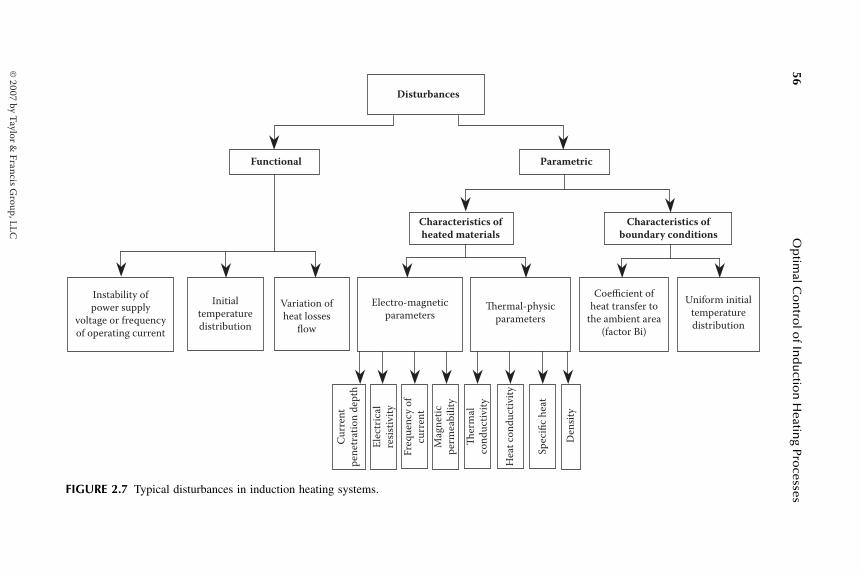
56O
ptim
al Co
ntro
l of In
du
ction
Heatin
g ProcessesFIGURE 2.7 Typical disturbances in induction heating systems.
Functional
Initial
temperature
distribution
Disturbances
Parametric
Variation of
heat losses
flow
Electro-magnetic
parameters Thermal-physic
parameters
Coefficient of
heat transfer to
the ambient area
(factor Bi)
Uniform initial
temperature
distribution
Characteristics of
heated materials
Characteristics of
boundary conditions
Mag
net
ic
per
mea
bil
ity
Ele
ctri
cal
resi
stiv
ity
Fre
qu
enc
y o
f
curr
ent
Cu
rren
t
pen
etra
tio
n d
epth
Instability of
power supply
voltage or frequency
of operating current
Ther
mal
con
du
ctiv
ity
Hea
t co
nd
uct
ivit
y
Sp
ecifi
c h
eat
Den
sity
DK
6039_C002.fm
Page 56 Friday, June 9, 2006 7:46 AM
© 2007 by Taylor &
Francis Group, LLC
Optimization Problems for Induction Heating Processes 57
; . (2.20)
Values of these disturbances are limited only by maximum and minimumvalues Bimin, Bimax and θ0min, θ0max, which usually can be calculated simply enoughfrom upper and lower limits of these parameters. Similar treatment should begiven to other parametric disturbances involved in OCP formulation.
2.7 REQUIREMENTS OF FINAL TEMPERATURE DISTRIBUTION WITHIN HEATED WORKPIECES
The ultimate goal of an induction heating process is obtaining desired temperaturedistribution within workpieces before subsequent technological operations. Thatis why proper formulation of the requirements to these temperature states is ofprimary importance. In most cases of induction heating of metals prior to hotworking, it is necessary to have uniform temperature distribution within the heatedworkpiece. Desired temperature depends on metal properties and specifics ofmetal hot working operations.
Mathematically speaking, this requirement of providing a uniform heatingcan be formulated as following: it is necessary to provide temperature uniformityat the level of prescribed value θ* = const at the end of heating process ϕ = ϕ0:
. (2.21)
However, due to the nature of induction heating, it is normally not possibleto obtain a perfectly uniform temperature distribution. One reason for that is anexistence of surface heat losses q(ϕ) < 0. Therefore, requirement (Equation 2.21)with regard to a perfectly uniform final temperature distribution is unrealizable.Indeed, if inequality q(ϕ0) < 0 in Equation (1.32) practically always remains true,then:
, (2.22)
That is why the temperature gradient on a workpiece surface always is negativeat the end of a heating process.
On the other hand, according to Equation (2.21), this gradient should be equalto zero for all values l, including l = 1 as well, which leads to contradiction. Thisproperty of an unattainability of final uniform temperature distribution (propertyof an uncontrollability of induction heating process) is a specific feature of aninduction heating process due to existence of internal heat sources.1
The condition of the uniform temperature distribution (Equation 2.21) appearstheoretically attainable for workpiece heating in installations with external heat
Bi Bi Bimin max≤ ≤ θ θ θ0 0 0min max≤ ≤
θ ϕ θ( , ) ;*l l0 0 1≡ ≤ ≤
∂∂
<θ ϕ( , )10
0
l
DK6039_C002.fm Page 57 Friday, June 9, 2006 7:46 AM
© 2007 by Taylor & Francis Group, LLC

58 Optimal Control of Induction Heating Processes
exchange (gas-fired furnaces, infrared and electric resistance furnaces, etc.).Therefore, the OCP for induction heating with the requirement (Equation 2.21)is unsolvable and should be considered as an ill-defined problem.
Evidently, it is necessary to “weaken” the condition in Equation (2.21), takinginto account practically always existing tolerances on the error (deviation)between actual final temperature distribution and desired distribution. In this case,a set of allowable temperature states (corresponding to given tolerance) shouldbe preset instead of fixed desired temperature distribution (Equation 2.21).
To provide a proper mathematical description of such a set, it is necessaryto define how the deviation from temperature distribution (Equation 2.21) shouldbe estimated. The most common approach might deal with estimation by rootmean square errors βms (within a volume of a heated body):
, (2.23)
where β*ms is an admissible value of βms, defined by given tolerances.
Moreover, estimation of accuracy by value βms is not in good compliancewith industrial technology requirements. In the most typical technological pro-cesses, maximum admissible value ε of absolute deviation of temperature distri-bution θ(l,ϕ0) from the required outlet temperature θ* is prescribed. This meansthat, at the end of a heating cycle, the temperature in any point of the billetvolume should deviate not more than by value ε from required temperature θ*:
. (2.24)
Thus, minimizing βms does not exclude inadmissible local deviations of finaltemperature arising from required one. This means that if Equation (2.23) is met,there is no assurance that necessary Equation (2.24) is complied with in somepoints l ∈ [0;1] (as a rule, on a surface of the heated body). At last, there are noeffective means to estimate acceptable values βms, starting from a practicallyrequired condition (Equation 2.24).
These statements prove that it is necessary to formulate requirements in theform of Equation (2.24) as close to actual technology as possible. Let us underlinethat, from the formal point of view, Equation (2.24) appears to be more compli-cated than the inequality in Equation (2.23). That is why only Expression (2.23)is used sometimes in engineering practice to simplify this problem. Instead ofEquation (2.24), the following inequality for maximum deviation on the interval[0,1] can be employed:
. (2.25)
β θ ϕ θ βms msl l dl= − ≤∫ ( , ) * *0 2
0
1
Γ
θ ϕ θ ε( , ) ,*l l0 0 1− ≤ ≤ ≤
max ( , )[ , ]
*
ll
∈− ≤
0 1
0θ ϕ θ ε
DK6039_C002.fm Page 58 Friday, June 9, 2006 7:46 AM
© 2007 by Taylor & Francis Group, LLC
Optimization Problems for Induction Heating Processes 59
Regarding the basic process model (Equation 1.27 through Equation 1.35),we shall consider requirements to temperature distribution at the end of a heatingcycle in the form Equation (2.25) everywhere below. Such distribution, θ(l,ϕ0),we shall call sometimes for short “final temperature distribution.” Substitutingthe variable in Equation (2.6) into Equation (2.25) results in the following formof the condition:
. (2.26)
Here, the radial temperature distribution (along coordinate l) at the heater exity = y0 is considered as final temperature distribution in steady-state mode ofcontinuous heater.
If requirements to final temperature distribution are included into cost func-tion, this means that an optimal control problem is reduced to minimizing devi-ation ε. In this case, it is not necessary to demand Equation (2.25) or any additionalrequirements of similar type.
Let us remark also that, for a number of technological processes, requirementsapplied to heating accuracy are weakened compared to Equation (2.25). In par-ticular, they can be limited to only a certain part of a heated workpiece (forexample, to surface layer) and/or required heating accuracy depends on spatialcoordinate l. In such cases, Equation (2.25) is stated as:
. (2.26a)
Here, the interval [l*; l**], 0 ≤ l* < l** ≤ 1 specifies depth and location of a layerwithin the boundaries of a heated workpiece for which requirements to finaltemperature state are set. Deviation ε(l) is a given (for example, linear) functionof coordinate l on interval [l*; l**].
2.8 GENERAL PROBLEM OF TIME-OPTIMAL CONTROL
In this section, we shall be concerned with the time-optimal control problem forthe heating process described previously. Application of obtained results to dif-ferent and more complex OCP statements is left to the following sections.
At first, we shall consider the most general optimal control problem, assumingthat complete information is available about the heating process and imposedrequirements. Let us also assume that there are no disturbances affecting theheating system and the time of workpiece transfer to hot working equipment isnegligible. We will also consider that an induction heating process is properlydescribed by Equation (1.27) through Equation (1.35). The workpiece temperature
max ,[ , ]
*
ll
y
V∈
− ≤
0 1
0
θ θ ε
max , ( )[ , ]
*
* **l l ll l
∈( ) − ≤θ ϕ θ ε0
DK6039_C002.fm Page 59 Friday, June 9, 2006 7:46 AM
© 2007 by Taylor & Francis Group, LLC

60 Optimal Control of Induction Heating Processes
distribution will be treated as an output controlled function of the process. Controlinput function is chosen from the set of admissible controls to influence temper-ature distribution and dynamic behavior of an induction heating system.
Let the control problem be formulated based upon the data presented inSection 2.2 through Section 2.7 as follows:
• The initial temperature state is defined as Equation (1.30) and requiredtemperature distribution is described by Equation (2.25).
• The control constraint set is given in a form of Equation (2.7), Equation(2.8), or Equation (2.10).
• The constraint on a temperature field can be written in one of the forms(Equation 2.11 through Equation 2.17).
• The cost function for each control input can be estimated by chosencriteria from the set (Equation 2.1 through Equation 2.5).
Then the statement of an optimal induction heating control problem can beformulated such as following. We wish to steer an initial workpiece temperaturestate to a desired target state and hold cost criteria at extremum value by space-time-varying control restricted by a preassigned set and satisfied by the constrainton a temperature field. The control input functions resulting from the precedingOCP solution are called optimal controls. To simplify the control problem, it willbe assumed that initial temperature distribution is uniform: θ0(l) ≡ 0 ≡ const. Asimilar statement can be made for large numbers of optimal control problems oftechnology and science.
Let us consider the simplest, most typical, and representative problem ofoptimal control for a static heating process. A mathematical model is describedby Equation (1.27) through Equation (1.35). Process time duration (Equation 2.1)can be considered as a cost criterion (problem of time-optimal control). Time-dependent heating power u(ϕ) is chosen as lumped control input restrained by(Equation 2.7). Technological constraints (Equation 2.11 through Equation 2.17)are not taken into account because it is assumed that they are complied with alladmissible controls. This control problem represents optimization of IHIs whenthe ultimate goal is to provide a maximum productivity under a prescribedtemperature state of a heated workpiece.
Therefore, it is necessary to select a control function u(ϕ) = u*(ϕ) that providessteering workpiece initial temperature distribution to desired temperature θ* withprescribed accuracy ε (according to Equation 2.25) in minimal optimal processtime. Control input is bounded by minimum and maximum allowable values Umax
and Umin = 0 (see Equation 2.7), and temperature field is described by Equation(1.27) through Equation (1.35).
Conventional induction heating technology represents heating when inductorvoltage is constant during the whole process. For the model (Equation 1.27through Equation 1.35), this heating mode corresponds to constant value ofheating power u(ϕ) = u0 = const. Thus, the value u0 should be chosen in such a
DK6039_C002.fm Page 60 Friday, June 9, 2006 7:46 AM
© 2007 by Taylor & Francis Group, LLC

Optimization Problems for Induction Heating Processes 61
way that, at the end of a heating cycle, the temperature difference across billetthickness does not exceed 2ε as Equation (2.25) requires (Figure 2.8, curves 1, 2).
Because the surface-to-core temperature difference, θ(1,ϕ0) – θ(0,ϕ0), is pro-portional during heating cycle to the power u0, we are forced to choose sufficientlylow heating power (smaller than Umax) to obtain allowable deviations ε from θ*.This results in increasing the required heating time ϕ0 (approximately in inverseproportion to u0), leading to a process that would not be optimal with respect tothe criterion in Equation (2.1). Heating time can be reduced when a two-stageprocess is applied. Figure 2.8 shows the typical time–temperature curves for two-stage static induction heating. As one can see, immediately after the beginningof heating with u(ϕ) ≡ Umax > u0, the surface temperature (curve 3) and averagetemperature (curve 5) begin to rise. In contrast, there is a time delay before thecore temperature (curve 4) starts to grow.
As soon as power is switched off during the second process stage, (u(ϕ) ≡0), the surface temperature rapidly decreases due to heat soaking towards a coolercore. A corresponding rise in the core temperature takes place during this stage.During the soaking stage, the surface-to-core temperature differential decreasesand the heated component approaches the temperature uniformity required forhot working.
The advantage of a two-stage process in comparison to a single-stage processdeals with lower value of ε (Figure 2.8), and optimal heating time decreases withincreasing value Umax. It is important to note that the soaking stage can beperformed when the heated workpiece is inside the induction coil and/or during
FIGURE 2.8 Time-temperature curves for one- and two-stage heating modes.
θ∗ + ε
θ∗ − ε
Min θMin θ
ϕ10 ϕ
20
Max θMax θ
θ
θ∗1
2
3
4
5
ϕ
ϕ
u Umax
u0
DK6039_C002.fm Page 61 Friday, June 9, 2006 7:46 AM
© 2007 by Taylor & Francis Group, LLC
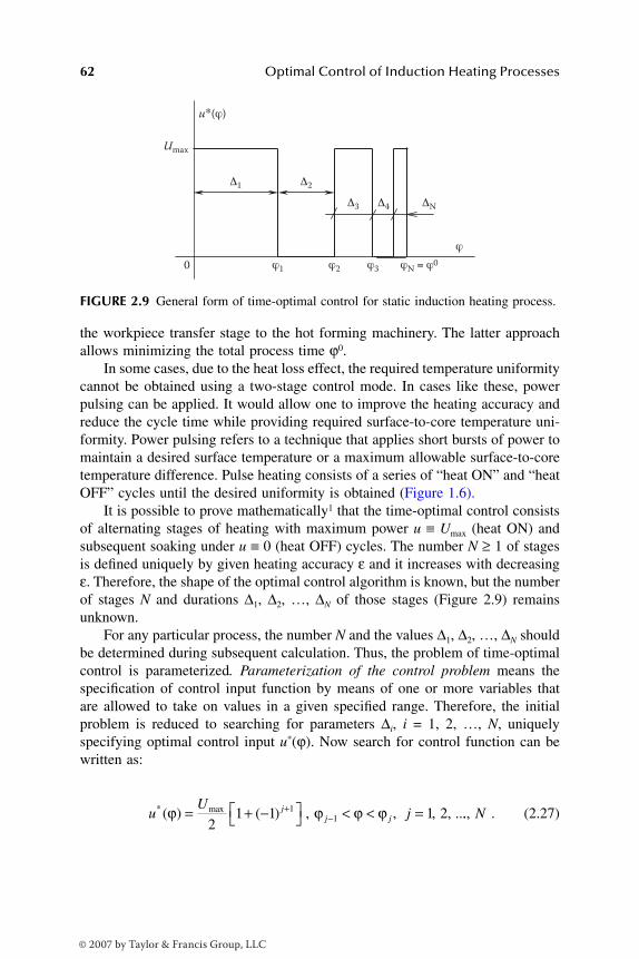
62 Optimal Control of Induction Heating Processes
the workpiece transfer stage to the hot forming machinery. The latter approachallows minimizing the total process time ϕ0.
In some cases, due to the heat loss effect, the required temperature uniformitycannot be obtained using a two-stage control mode. In cases like these, powerpulsing can be applied. It would allow one to improve the heating accuracy andreduce the cycle time while providing required surface-to-core temperature uni-formity. Power pulsing refers to a technique that applies short bursts of power tomaintain a desired surface temperature or a maximum allowable surface-to-coretemperature difference. Pulse heating consists of a series of “heat ON” and “heatOFF” cycles until the desired uniformity is obtained (Figure 1.6).
It is possible to prove mathematically1 that the time-optimal control consistsof alternating stages of heating with maximum power u ≡ Umax (heat ON) andsubsequent soaking under u ≡ 0 (heat OFF) cycles. The number N ≥ 1 of stagesis defined uniquely by given heating accuracy ε and it increases with decreasingε. Therefore, the shape of the optimal control algorithm is known, but the numberof stages N and durations ∆1, ∆2, …, ∆N of those stages (Figure 2.9) remainsunknown.
For any particular process, the number N and the values ∆1, ∆2, …, ∆N shouldbe determined during subsequent calculation. Thus, the problem of time-optimalcontrol is parameterized. Parameterization of the control problem means thespecification of control input function by means of one or more variables thatare allowed to take on values in a given specified range. Therefore, the initialproblem is reduced to searching for parameters ∆i, i = 1, 2, …, N, uniquelyspecifying optimal control input u*(ϕ). Now search for control function can bewritten as:
. (2.27)
FIGURE 2.9 General form of time-optimal control for static induction heating process.
Δ1 Δ2
Δ3 Δ4 ΔN
0
u∗(ϕ)
ϕ1
ϕ
ϕ2 ϕ3 ϕN = ϕ0
Umax
uU
jjj j
* max( ) ( ) , , , , ..ϕ ϕ ϕ ϕ= + − < < =+−2
1 1 1 211 .., N
DK6039_C002.fm Page 62 Friday, June 9, 2006 7:46 AM
© 2007 by Taylor & Francis Group, LLC
Optimization Problems for Induction Heating Processes 63
Here, ϕj is the end point of the jth stage (jth point of control switch).
Obviously, ; we assume that ϕ0 = 0. According to Equation (2.27),
during any stage with an odd number (i.e., with odd number j), u*(ϕ) = Umax and,during an even stage, u*(ϕ) = 0 (Figure 2.9). In particular, for the appropriatevalues ε, Expression (2.27) describes a two-stage process of heating if N = 2, ∆1
= ϕ1, ∆2 = ϕ0 – ϕ1. It will be shown further that, for conventional heat lossesfrom the workpiece surface and typical requirements to heating accuracy, thetwo-stage control algorithm (Equation 2.27) usually represents the time-optimalheating mode.
If initial temperature and heat losses are known and assuming applying acontrol input (Equation 2.27), at the end of the heating cycle (at ϕ = ϕ0 = ϕN)the temperature in any point l ∈ [0,1] depends only on values ∆i, i = 1, 2, …, N.This means that θ(l,ϕ0) in Equation (2.25) is described by relation θ(l,∆), where∆ = (∆i), i = is a set of ∆i (∆ — vector of time intervals of all control stages[Figure 2.9]). By substituting u(ϕ) in Equation (2.27) and taking into consider-ation initial and boundary conditions (Equation 1.30 through Equation 1.34), thisexpression can be obtained in an explicit form as a solution of the heat conductionequation (Equation 1.27) for ϕ = ϕN.
In a case (Equation 1.34 and Equation 2.19) when initial temperature distri-bution is assumed to be uniform, θ0(l) ≡ θ0 = θa = const (this corresponds to aconstant ambient temperature θa), the solution can be written as1:
. (2.28)
Here, is a temperature in the point l at the time
when the control function takes on maximum allowable value (i.e., heating poweris maximum: u(ϕ) ≡ Umax) and θ0 = 0. Function Λ(l,ϕ) is called the responsefunction — i.e., the output from a heating process (Equation 1.27 through Equa-tion 1.35), which is obtained in response to applied input u(ϕ) ≡ 1 under θ0 = 0.
For the model (Equation 1.27 through Equation 1.35), response functionΛ(l,ϕ) can be calculated using the relation in Equation (1.40) as:
. (2.29)
ϕ j i
i
j
==∑∆
1
1, N
θ ϕ θ θ( , ) ( , ) ( ) ,maxl l U lmi
i m
N
00
11≡ = + −
+
=∑∆ Λ ∆
=∑m
N
1
U l i
i m
N
max ,Λ ∆=∑
ϕ ==∑∆i
i m
N
ΛΓ
lW K l
Bi Bi Kn n
n n
,( ) ( )
( ( ) ) ( )(ϕ ξ µ
µ µ( ) =
+ + −2
12 2 2 112
1
− −
=
∞
∑ e n
n
µ ϕ )
DK6039_C002.fm Page 63 Friday, June 9, 2006 7:46 AM
© 2007 by Taylor & Francis Group, LLC

64 Optimal Control of Induction Heating Processes
Therefore, the response function represents the infinite sum of exponents withdifferent factors for each value l. All notations used in the expression for thesefactors were explained in Section 1.2.2.
It is clear that in engineering practice, only a finite number of members inconvergent series (Equation 2.29) is always regarded. Thus, the condition (Equa-tion 2.25) required for a given final temperature state can be rewritten as:
, (2.30)
where θ(l,∆) is defined by Expression (2.28) and Expression (2.29).The problem now is reduced to determination of such time intervals, ∆i,
i = , of alternating heating and soaking stages that provide satisfying require-ments (Equation 2.30) in minimal possible time. Total time is equal to the sumof all ∆i . Then, a cost criterion can be determined as a following sum:
, (2.31)
where the minimum is taken over all admissible vectors ∆.From the formal point of view, the optimal control problem is reduced to a
mathematical programming problem minimizing an object function (Equation2.31) of N variables, ∆i, where restraint on a set of admissible values, ∆I, isprescribed in the form of Equation (2.30). As it was shown earlier, the inequality(Equation 2.30) represents a set of infinite number of constraints in a form ofEquation (2.24) for each of values l ∈ [0,1]. Therein lies a principal differenceof a problem (Equation 2.30 and Equation 2.31) compared to classical mathe-matical programming problems, in which only the finite constraints number isconsidered.
Let us recall also that a priori unknown number N of sought parameters shouldbe found in the course of the problem (Equation 2.30 and Equation 2.31) solution;this number N depends on prescribed value ε in Equation (2.30). It adds additionalcomplexity to this problem compared to a conventional one.
For a steady-state process of continuous heating described by Equation (1.27)through Equation (1.35) and Equation (2.6), substitution of a variable (Equation2.6) results in optimal spatial distribution of power u*(y/V) along heater length.The curve shown in Figure 2.9 is practically identical for continuous heatingmodes. In case of continuous heating, the time axis represents the length of theinduction heating line or coil length. Bursts of power can represent the power ofinline coils, which may have different length, windings, and/or can be individuallyfed from different power supplies. Under constraint (Equation 2.8), optimal heatpower distribution can be represented as a stepwise function in the form (Equation2.27) (Figure 2.10):
Φ ∆ ∆( ) max ( , )[ , ]
*= − ≤∈l
l0 1
θ θ ε
1, N
I i
i
N
( ) min∆ ∆∆
= →=∑
1
DK6039_C002.fm Page 64 Friday, June 9, 2006 7:46 AM
© 2007 by Taylor & Francis Group, LLC
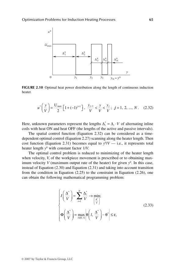
Optimization Problems for Induction Heating Processes 65
. (2.32)
Here, unknown parameters represent the lengths of alternating inlinecoils with heat ON and heat OFF (the lengths of the active and passive intervals).
The spatial control function (Equation 2.32) can be considered as a time-dependent optimal control (Equation 2.27) scanning along the heater length. Thencost function (Equation 2.31) becomes equal to y0/V — i.e., it represents totalheater length y0 with constant factor 1/V.
The optimal control problem is reduced to minimizing of the heater lengthwhen velocity, V, of the workpiece movement is prescribed or to obtaining max-imum velocity V (maximum output rate of the heater) for given y0. In this case,instead of Equation (2.30) and Equation (2.31) and taking into account transitionfrom the condition in Equation (2.25) to the constraint in Equation (2.26), onecan obtain the following mathematical programming problem:
(2.33)
FIGURE 2.10 Optimal heat power distribution along the length of continuous inductionheater.
0
u∗
Δ∗1 Δ∗2
Δ∗3 Δ∗4 Δ∗N
y1 y2 y3
y yN = y0
Umax
uy
V
y
V
y
V
y
Vj j j* ( ) , ;
= + − < <+ −Umax
21 1 1 1 jj N= 1, 2, ...,
∆ ∆i i V* = ⋅
IV V
V
i
i
N
V
∆ ∆
Φ ∆
∆
* *
*
min;*
= →
=
∑1
=
− ≤
∈
max , ,*
*
ll
V[0, 1]θ θ ε∆
DK6039_C002.fm Page 65 Friday, June 9, 2006 7:46 AM
© 2007 by Taylor & Francis Group, LLC

66 Optimal Control of Induction Heating Processes
where , and the expressions for are deter-
mined by Expression (2.28) and Expression (2.29) by substituting .
Let us assume at this point that Equation (2.30), Equation (2.31), and Equation(2.33) are solvable — i.e., the required controlled temperature distribution canbe obtained by admissible control function applied to the heating system. Here,it is still assumed that optimal control mode consists of N alternating stages ofheating and temperature soaking and that number N is a priori known. Further-more, we shall discuss how N can be defined depending on required permissiblevalue ε and how the conditions of attainability are set. We shall also extend ourresults to the solution of similar problems. Advantages of an optimal controlmethod compared to known numerical methods will be shown as well.
2.9 MODEL PROBLEMS OF OPTIMAL CONTROL RESPECTIVE TO TYPICAL COST FUNCTIONS
In the previous section, it has been shown that the general problem of time-optimal control of an induction heating process described by Equation (1.27)through Equation (1.35) is reduced to a special problem of mathematical pro-gramming in the form of Equation (2.30) and Equation (2.31):
(2.34)
As we shall see, a whole class of optimization problems can be solved in themanner indicated: problems that involve the typical cost criteria while the processis described by the model (Equation 1.27 through Equation 1.35).
2.9.1 PROBLEM OF ACHIEVING MAXIMUM HEATING ACCURACY
Among typical cost criteria (accepted for static and continuous induction heatingprocesses), an important cost function is defined as error between the requiredtemperature distribution and the actual one obtained at the end of the heatingcycle (Section 2.2). Everywhere else such error is called heating accuracy, which,according to Equation (2.25) (see Section 2.7), is estimated by absolute deviation,ε, from the desired temperature state.
If Equation (2.25) is true for certain ε = ε1, then it remains true for all ε >ε1 at the same value of ϕ0. Therefore, minimal heating time 0ϕmin decreases as ε
∆ ∆ ∆ ∆* * * *
, ,...,V V V V
N=
1 2 θ l
V,
*∆
∆ ∆i
i
V=
*
I
l
i
i
N
l
∆ ∆
Φ ∆ ∆
∆( ) = →
( ) = ( ) − ≤
=
∈
∑1
min;
max , *
[0, 1]θ θ εε.
DK6039_C002.fm Page 66 Friday, June 9, 2006 7:46 AM
© 2007 by Taylor & Francis Group, LLC
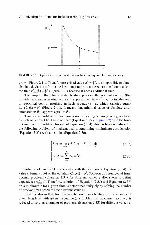
Optimization Problems for Induction Heating Processes 67
grows (Figure 2.11). Then, for prescribed value , it is impossible to obtainabsolute deviation ε from a desired temperature state less than attainable atthe time (Figure 2.11) because it needs additional time.
This implies that, for a static heating process, the optimal control (thatprovides maximum heating accuracy at prescribed time ) coincides withtime-optimal control resulting in such accuracy , which satisfies equal-ity (Figure 2.11). It means that minimal value of absolute error,attainable in , appears equal to .
Thus, in the problem of maximum absolute heating accuracy for a given time,the optimal control has the same form (Equation 2.27) (Figure 2.9) as in the time-optimal control problem. Instead of Equation (2.34), this problem is reduced tothe following problem of mathematical programming minimizing cost function(Equation 2.35) with constraint (Equation 2.36):
(2.35)
(2.36)
Solution of this problem coincides with the solution of Equation (2.34) forvalue ε being a root of the equation . Solution of a number of time-optimal problems (Equation 2.34) for different values ε allows one to definedependence 0ϕmin(ε). Therefore, solution of Equation (2.35) and Equation (2.36)on a minimum ε for a given time is determined uniquely by solving the numberof time-optimal problems for different values ε.
It can be shown that, for steady-state continuous heating (in the inductor ofgiven length y0 with given throughput), a problem of maximum accuracy isreduced to solving a number of problems (Equation 2.33) for different values ε.
FIGURE 2.11 Dependence of minimal process time on required heating accuracy.
ϕ0min
ε~
ϕ0~
ε
ϕ ϕ0 0= ε ε=
ϕ ε ϕmin ( )0 0 =
ϕ ϕ0 = ε ε=
ϕ ε ϕmin ( )0 0 =ϕ0 ε
I ll
i
i
N
∆ ∆
Φ ∆ ∆
∆( ) = ( ) − →
( ) = =
∈
=∑
max , min;*
[0, 1]θ θ
1
ϕ0 .
ϕ ε ϕmin ( )0 0=
DK6039_C002.fm Page 67 Friday, June 9, 2006 7:46 AM
© 2007 by Taylor & Francis Group, LLC

68 Optimal Control of Induction Heating Processes
In total, this problem, like Equation (2.35) and Equation (2.36), can be writtenas follows:
(2.37)
Here, all notations correspond to those for Equation (2.33).Chosen voltages U1, U2, …, UN (or corresponding heat powers u1, u2, …, uN)
for all N coils of the multicoil continuous heater can be considered as parametricspatial controls in Equation (2.9) (Section 2.4 and Section 2.5). Then, the fol-lowing modification of the problem of maximum accuracy can be obtained forsteady-state continuous heating similarly to Equation (2.35) and Equation (2.37):
. (2.38)
Here, U = (U1, U2, …, UN); voltages U1, U2, …, UN (or powers u1, u2, …, uN forseparate coils) are sought parameters instead of ∆1, ∆2, …, ∆N in Equation (2.35)and Equation (2.36) or *∆i /V in Equation (2.37). At least at the first stage, addi-tional constraints are not taken into account, in contrast to Equation (2.35) throughEquation (2.37).
The function θ(l,U) in Equation (2.38) is similar to θ(l,∆*/V) in Equation(2.37). This expression represents a temperature distribution along radial coordi-nate l at the heater exit y = y0. It is determined uniquely by vector of parametersU. Similarly to Equation (2.28), after substitution (2.6), this relation can beobtained in explicit form as solution of the heat conduction equation (Equation1.27) with boundary and initial conditions (Equation 1.30 through Equation 1.34).
For the linear process model (Equation 1.27 through Equation 1.35) andneglecting any air gaps between induction coils, a distribution, u(y), of internalheat power along the inductor length can be represented as a step function shownin Figure 2.12.
For constant voltage on each coil, the intensity of heat generation caused byan electromagnetic field is assumed constant along the whole coil length. In thiscase, the value of heating power for each coil is considered as unknown parameter.At the same time, the lengths of each coil are predetermined by coordinates y1,y2, …, yN. This case differs from the one presented in Figure 2.10, in which forprescribed value Umax, it is necessary to define lengths *∆1, *∆2, …, *∆N of intervalswith given heat powers.
It should be mentioned that the control algorithm (Equation 2.32) shown inFigure 2.10 allows using only on–off power control because there are only two
I lVl
V
i
i
∆ ∆
∆
∆( ) =
− →
∈
=
max , min ;*
*
*
*[0, 1]θ θ
11
0N
y∑ =
.
I U l Ul U
( ) = ( ) − →∈max , min*
[0, 1]θ θ
DK6039_C002.fm Page 68 Friday, June 9, 2006 7:46 AM
© 2007 by Taylor & Francis Group, LLC
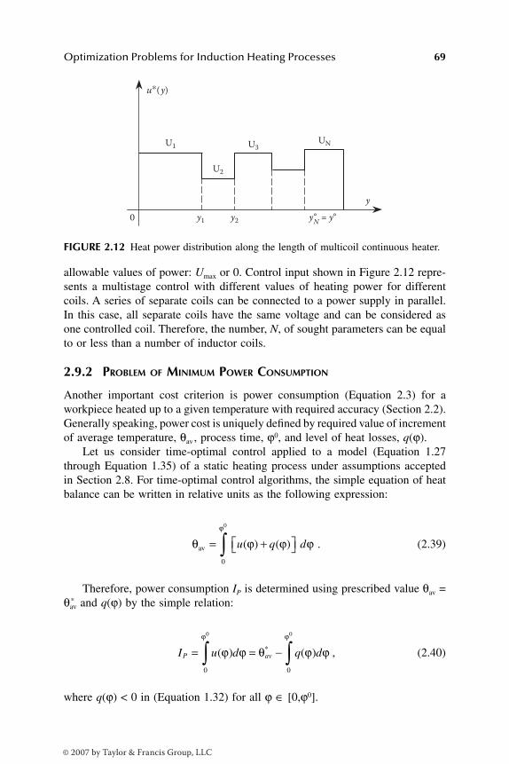
Optimization Problems for Induction Heating Processes 69
allowable values of power: Umax or 0. Control input shown in Figure 2.12 repre-sents a multistage control with different values of heating power for differentcoils. A series of separate coils can be connected to a power supply in parallel.In this case, all separate coils have the same voltage and can be considered asone controlled coil. Therefore, the number, N, of sought parameters can be equalto or less than a number of inductor coils.
2.9.2 PROBLEM OF MINIMUM POWER CONSUMPTION
Another important cost criterion is power consumption (Equation 2.3) for aworkpiece heated up to a given temperature with required accuracy (Section 2.2).Generally speaking, power cost is uniquely defined by required value of incrementof average temperature, θav , process time, ϕ0, and level of heat losses, q(ϕ).
Let us consider time-optimal control applied to a model (Equation 1.27through Equation 1.35) of a static heating process under assumptions acceptedin Section 2.8. For time-optimal control algorithms, the simple equation of heatbalance can be written in relative units as the following expression:
. (2.39)
Therefore, power consumption IP is determined using prescribed value θav =θav
* and q(ϕ) by the simple relation:
, (2.40)
where q(ϕ) < 0 in (Equation 1.32) for all ϕ ∈ [0,ϕ0].
FIGURE 2.12 Heat power distribution along the length of multicoil continuous heater.
U1
U2
y1 y2
y y°N = y°
U3 UN
0
u∗( y)
θ ϕ ϕ ϕϕ
av = + ∫ u q d( ) ( )0
0
I u d q dP av= = −∫ ∫( ) ( )*ϕ ϕ θ ϕ ϕϕ ϕ
0 0
0 0
DK6039_C002.fm Page 69 Friday, June 9, 2006 7:46 AM
© 2007 by Taylor & Francis Group, LLC

70 Optimal Control of Induction Heating Processes
Thus, it follows that cost of required power is reduced with decreasing ofprocess time due to decreasing heat losses taken into account by an integral inthe right side of Equation (2.40). Starting from Equation (2.40), this means thatthe heating mode with constant maximum permissible power u(ϕ) = u*(ϕ) ≡ Umax
during the whole process would be optimal with respect to criterion IP .As has been shown in Section 2.8, the algorithm u*(ϕ) ≡ Umax does not always
provide the final required temperature accuracy ε. Obviously, in this case, controlinput, u*(ϕ), would be optimal with respect to energy consumption at givenaccuracy ε if control function u*(ϕ) is of the same form as well as time-optimalcontrol with alternating intervals of heating with maximum power u*(ϕ) ≡ Umax
and soaking stage u*(ϕ) ≡ 0 (Section 2.8, Figure 2.8). During intervals with u*(ϕ)≡ 0, power consumption is equal to 0 and, during intervals with u*(ϕ) ≡ Umax,appropriate increase of average temperature is reached in the fastest possible way— i.e., with minimum power consumption.
Generally speaking, the similar mode is optimal with respect to criterionIP under required heating accuracy ε. Presented substantiation is proved bymathematical analysis,1 which determines single-type (ON–OFF) optimal con-trol by power of internal heat sources for static induction heating processes.Control input of this type is optimal with respect to both criteria: minimumtime and minimum power consumption. However, generally speaking, it doesnot mean that these optimal controls completely coincide for the same pre-scribed values ε.
Note that, in many cases, time optimal and power-optimal control inputs inthe form of Equation 2.27 correspond to different time periods ∆i , i = 1, 2, …,N and different number N of constancy intervals (Figure 2.9). For example, ifrequired accuracy ε = ε0 is reached in a “one-stage” heating process with constantpower, u(ϕ) ≡ Umax, over total process time, then this control would be time-optimal for this value ε. The same accuracy, but with less power consumption,could be achieved in “two-stage” mode by decreasing duration of the first intervalwith u(ϕ) ≡ Umax and adding the second interval for temperature leveling withu(ϕ) ≡ 0, when power consumption is zero. In this case, the temperature drop atthe end of heating will decrease until the required level owing to increase of thetotal process time.
As one can see, considered optimal control algorithms that belong to oneclass of control inputs can differ from one another by particular values of appro-priate parameters. As will be shown further, this does not exclude situations whenthere is a full coincidence of time-optimal control with power-optimal controlfor certain requirements to heating accuracy.
Under heating power control in Equation (2.27), power costs (Equation 2.40)are proportional to the sum of odd control intervals instead of the sum (Equation2.31) of all control intervals for the time-optimal problem. Then, an optimizationcriterion could be written as:
DK6039_C002.fm Page 70 Friday, June 9, 2006 7:46 AM
© 2007 by Taylor & Francis Group, LLC
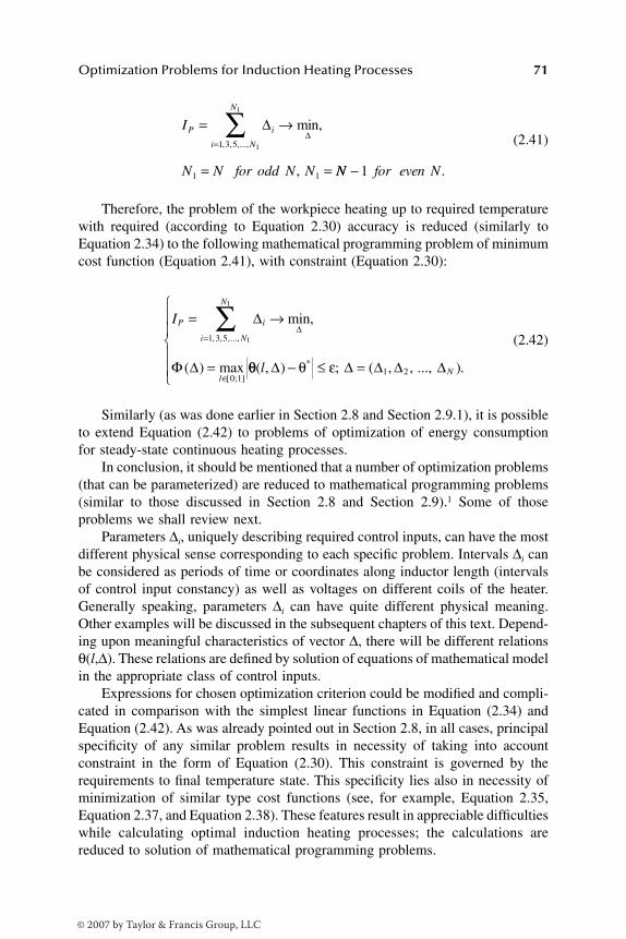
Optimization Problems for Induction Heating Processes 71
(2.41)
Therefore, the problem of the workpiece heating up to required temperaturewith required (according to Equation 2.30) accuracy is reduced (similarly toEquation 2.34) to the following mathematical programming problem of minimumcost function (Equation 2.41), with constraint (Equation 2.30):
(2.42)
Similarly (as was done earlier in Section 2.8 and Section 2.9.1), it is possibleto extend Equation (2.42) to problems of optimization of energy consumptionfor steady-state continuous heating processes.
In conclusion, it should be mentioned that a number of optimization problems(that can be parameterized) are reduced to mathematical programming problems(similar to those discussed in Section 2.8 and Section 2.9).1 Some of thoseproblems we shall review next.
Parameters ∆i, uniquely describing required control inputs, can have the mostdifferent physical sense corresponding to each specific problem. Intervals ∆i canbe considered as periods of time or coordinates along inductor length (intervalsof control input constancy) as well as voltages on different coils of the heater.Generally speaking, parameters ∆i can have quite different physical meaning.Other examples will be discussed in the subsequent chapters of this text. Depend-ing upon meaningful characteristics of vector ∆, there will be different relationsθ(l,∆). These relations are defined by solution of equations of mathematical modelin the appropriate class of control inputs.
Expressions for chosen optimization criterion could be modified and compli-cated in comparison with the simplest linear functions in Equation (2.34) andEquation (2.42). As was already pointed out in Section 2.8, in all cases, principalspecificity of any similar problem results in necessity of taking into accountconstraint in the form of Equation (2.30). This constraint is governed by therequirements to final temperature state. This specificity lies also in necessity ofminimization of similar type cost functions (see, for example, Equation 2.35,Equation 2.37, and Equation 2.38). These features result in appreciable difficultieswhile calculating optimal induction heating processes; the calculations arereduced to solution of mathematical programming problems.
I
N N for odd N N
P i
i N
N
= →
= =
=∑ ∆
∆1 3 5
1 1
1
1
, , ,...,
min,
, NN for even N− 1 .
IP i
i N
N
l
= →
=
=
∈
∑ ∆
Φ ∆
∆1 3 5
0 1
1
1
, , ,...,
[ ; ]
min,
( ) max θθ θ ε( , ) ; ( , , ..., ).*l N∆ ∆ ∆ ∆ ∆− ≤ =
1 2
DK6039_C002.fm Page 71 Friday, June 9, 2006 7:46 AM
© 2007 by Taylor & Francis Group, LLC
72 Optimal Control of Induction Heating Processes
Known formal techniques for such solution are reduced to relatively compli-cated numerical methods; their general orientation is not connected to specificcontent of the problem. An alternative effective approach to this problem issuggested in the following chapter. It is based on physical properties of investi-gated heating systems and offers many opportunities for development of simpleand effective engineering techniques of optimized process computation.1,8
REFERENCES
1. Rapoport, E.Ya., Optimization of Induction Heating of Metals, Metallurgy, Mos-cow, 1993.
2. Butkovskij, A.G., Malyj, S.A., and Andreev, Yu.N., Optimal Control of MetalsHeating, Metallurgy, Moscow, 1972.
3. Butkovskij, A.G., Malyj, S.A., and Andreev, Yu.N., Control of Metals Heating,Metallurgy, Moscow, 1981.
4. Rudnev, V.I. et al., Handbook of Induction Heating, Marcel Dekker, New York,2003.
5. Nemkov, V.S. and Demidovich, V.B., Theory and Computation of Induction Heat-ing Installations, Energoatomizdat, St. Petersburg, 1988.
6. Pavlov, N.A., Engineering Thermal Computation of Induction Heaters, Energia,Moscow, 1978.
7. Sluhotskii, A.E. et al., Induction Heating Installations, Energoatomizdat, St. Peters-burg, 1981.
8. Rapoport, E.Ya., Alternate Method for Solving Applied Optimal Control Problems,Nauka, Moscow, 2000.
DK6039_C002.fm Page 72 Friday, June 9, 2006 7:46 AM
© 2007 by Taylor & Francis Group, LLC

73
3
Method for Computation of Optimal Processes for Induction Heating of Metals
This chapter delves into basics of a new optimal control method that allows oneto solve a wide range of optimization problems for induction heating of metalsprior to hot forming. The new optimization technique is called the “alternancemethod.” This method is based on qualitative features of temperature distributionwithin the heated workpiece at the end of the optimal heating process. Thesefeatures have clear physical meaning and are similar to properties of the bestuniform approximation of given functions to zero.
1
To explain new optimal controltechniques in clear and simple form it is reasonable to consider only the generalproblem of time-optimal control for the static heating process
2–5
(see Section 2.8).Subsequent chapters will show how to extend the suggested method to the solutionof other optimization problems.
3.1 UNIVERSAL PROPERTIES OF TEMPERATURE DISTRIBUTION WITHIN WORKPIECES AT END OF TIME-OPTIMAL INDUCTION HEATING PROCESSES
As has been discussed in Section 2.8, the time-optimal control algorithm
u
*
(
ϕ
)of the static induction heating process is defined as a step function (Equation2.27) with
N
≥
1 intervals of constancy (Figure 2.9), where
u
*
(
ϕ
) is an internalheat power. Therefore, the time-optimal control consists of alternating stages ofheating with maximum power
u
≡
U
max
(“heat ON”) and subsequent soaking(“heat OFF”) under
u
≡
0 cycles. The number of stages (
N
≥
1) is defined uniquelyby given heating accuracy
ε
. Smaller
ε
requires a larger number of stages,
N
.Therefore, the shape of the optimal control algorithm is known, but the number
N
and time durations
∆
1
,
∆
2
, …,
∆
N
of the described stages (Figure 2.9) remainunknown.
For any particular process, the number
N
and the values
∆
1
,
∆
2
, …,
∆
N
couldbe determined during subsequent computations. Particular values of these vari-ables depend on required accuracy
ε
of approximation to prescribed final tem-perature distribution (according to Equation 2.30).
DK6039_C003.fm Page 73 Monday, June 12, 2006 10:22 AM
© 2007 by Taylor & Francis Group, LLC
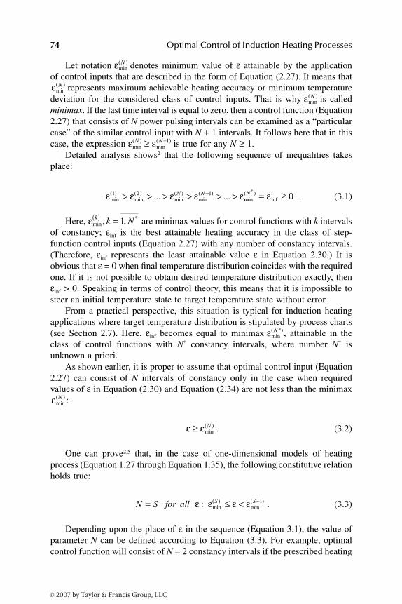
74
Optimal Control of Induction Heating Processes
Let notation denotes minimum value of
ε
attainable by the applicationof control inputs that are described in the form of Equation (2.27). It means that
represents maximum achievable heating accuracy or minimum temperaturedeviation for the considered class of control inputs. That is why is called
minimax
. If the last time interval is equal to zero, then a control function (Equation2.27) that consists of
N
power pulsing intervals can be examined as a “particularcase” of the similar control input with
N
+ 1 intervals. It follows here that in thiscase, the expression
≥
is true for any
N
≥
1. Detailed analysis shows
2
that the following sequence of inequalities takesplace:
. (3.1)
Here, are minimax values for control functions with
k
intervalsof constancy;
ε
inf
is the
best attainable heating accuracy in the class of step-function control inputs (Equation 2.27) with any number of constancy intervals.(Therefore,
ε
inf
represents the least attainable value
ε
in Equation 2.30.) It isobvious that
ε
= 0 when final temperature distribution coincides with the requiredone. If it is not possible to obtain desired temperature distribution exactly, then
ε
inf
> 0. Speaking in terms of control theory, this means that it is impossible tosteer an initial temperature state to target temperature state without error.
From a practical perspective, this situation is typical for induction heatingapplications where target temperature distribution is stipulated by process charts(see Section 2.7). Here,
ε
inf
becomes equal to minimax , attainable in theclass of control functions with
N
*
constancy intervals, where number
N
*
isunknown a priori.
As shown earlier, it is proper to assume that optimal control input (Equation2.27) can consist of
N
intervals of constancy only in the case when requiredvalues of
ε
in Equation (2.30) and Equation (2.34) are not less than the minimax:
. (3.2)
One can prove
2,5
that, in the case of one-dimensional models of heatingprocess (Equation 1.27 through Equation 1.35), the following constitutive relationholds true:
. (3.3)
Depending upon the place of
ε
in the sequence (Equation 3.1), the value ofparameter
N
can be defined according to Equation (3.3). For example, optimalcontrol function will consist of
N
= 2 constancy intervals if the prescribed heating
εmin( )N
εmin( )N
εmin( )N
εmin( )N εmin
( )N+1
ε ε ε ε εmin( )
min( )
min( )
min( )... ...1 2 1> > > > > >+N N
mmin( )
inf
*N = ≥ε 0
εmin*, ,k k N( ) = 1
εmin( *)N
εmin( )N
ε ε≥ min( )N
N S for all S S= ≤ < −ε ε ε ε: min( )
min( )1
DK6039_C003.fm Page 74 Monday, June 12, 2006 10:22 AM
© 2007 by Taylor & Francis Group, LLC

Computation of Optimal Processes for Induction Heating of Metals
75
accuracy is equal to or it is within the limits between and (i.e.,
≤
ε
< ). If the required value
ε
equals , then, according to the samerule (Equation 3.3), the value of
N
will be as
N
= 1.The values of minimaxes in the sequence of inequalities (Equation 3.1) are
unknown a priori. Therefore, it is impossible to determine in advance that theconditions in Equation (3.2) and Equation (3.3) will be satisfied for the prescribedvalue of
ε
. For that reason, the values for different
N
should be included inthe set of unknown parameters of optimal process
.
Optimal control, being the solution of the considered time-optimal problem,has definite set of intervals
0
∆
1
,
0
∆
2
, …,
0
∆
N
. Therefore, the vector
∆
0
=
0
(
∆
1
,
0
∆
2
, …,
∆
N
)
0
represents the solution of the mathematical programming problem in Equa-tion (2.34). All control inputs consisting of
N
constancy intervals with timeperiods
∆
≠
∆
0
should not be considered as optimal. Spatial temperature distri-bution
θ
(
l
,
∆
0
) at the end of an optimal process is a response to vector
∆
0
andshould satisfy the constraint (Equation (2.30)) in Equation (2.34). The temperaturedistribution
θ
(
l
,
∆
0
) differs from all other final temperature distributions
θ
(
l
,
∆
) (for
∆
≠
∆
0
) by several important properties. The suggested method takes theseproperties for solving any time-optimal problems of the type of Equation (2.34)into consideration.
Restraint (Equation 2.30), imposed on temperature distribution
θ
(
l
,
∆
0
), meansthat absolute deviations
θ
(
l
,
∆
0
) –
θ
*
of final temperature from the required oneshould not exceed the prescribed value of
ε
for all spatial coordinates,
l
∈
[0; 1].These deviations prove to be strictly less than
ε
on interval [0; 1]
∋
l
(Figure 3.1,curve 1), or they become strictly equal to ε in separate points (one or more) ofmaximum deviations within the same interval (Figure 3.1, curves 2 through 4).
FIGURE 3.1 Possible variants of temperature distribution across workpiece thickness atthe end of heating up to desired temperature θ* with required accuracy ε.
εmin( )2 εmin
( )2 εmin( )1
εmin( )2 εmin
( )1 εmin( )1
εmin( )N
0 1
l
1
2
3
θ∗ + ε
θ∗ − ε
4θ∗
θ(l, ∆0)
DK6039_C003.fm Page 75 Monday, June 12, 2006 10:22 AM
© 2007 by Taylor & Francis Group, LLC
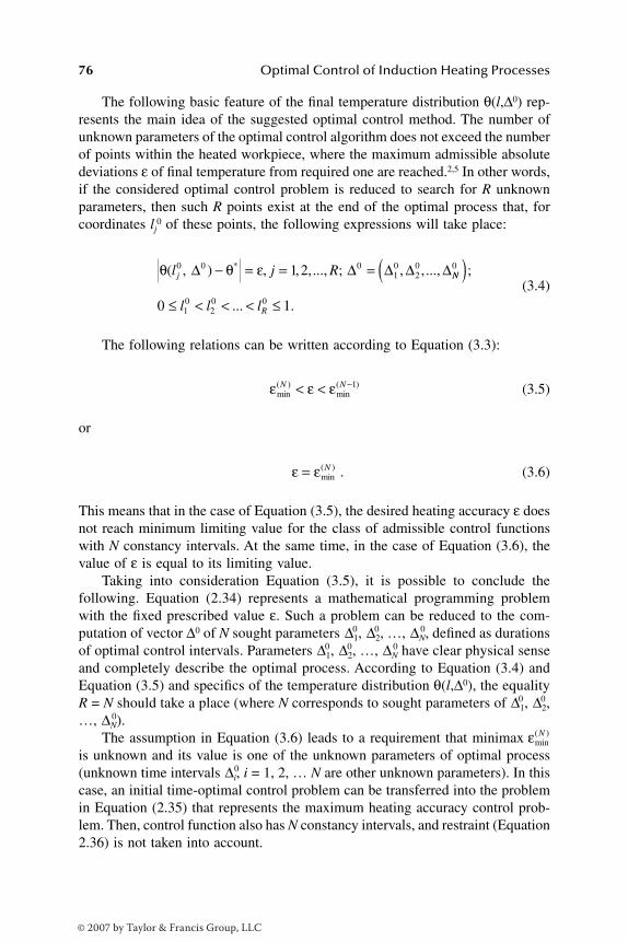
76 Optimal Control of Induction Heating Processes
The following basic feature of the final temperature distribution θ(l,∆0) rep-resents the main idea of the suggested optimal control method. The number ofunknown parameters of the optimal control algorithm does not exceed the numberof points within the heated workpiece, where the maximum admissible absolutedeviations ε of final temperature from required one are reached.2,5 In other words,if the considered optimal control problem is reduced to search for R unknownparameters, then such R points exist at the end of the optimal process that, forcoordinates lj
0 of these points, the following expressions will take place:
(3.4)
The following relations can be written according to Equation (3.3):
(3.5)
or
. (3.6)
This means that in the case of Equation (3.5), the desired heating accuracy ε doesnot reach minimum limiting value for the class of admissible control functionswith N constancy intervals. At the same time, in the case of Equation (3.6), thevalue of ε is equal to its limiting value.
Taking into consideration Equation (3.5), it is possible to conclude thefollowing. Equation (2.34) represents a mathematical programming problemwith the fixed prescribed value ε. Such a problem can be reduced to the com-putation of vector ∆0 of N sought parameters 0∆1,
0∆2, …, 0∆N, defined as durationsof optimal control intervals. Parameters 0∆1,
0∆2, …, 0∆N have clear physical senseand completely describe the optimal process. According to Equation (3.4) andEquation (3.5) and specifics of the temperature distribution θ(l,∆0), the equalityR = N should take a place (where N corresponds to sought parameters of 0∆1,
0∆2,…, 0∆N).
The assumption in Equation (3.6) leads to a requirement that minimaxis unknown and its value is one of the unknown parameters of optimal process(unknown time intervals 0∆i, i = 1, 2, … N are other unknown parameters). In thiscase, an initial time-optimal control problem can be transferred into the problemin Equation (2.35) that represents the maximum heating accuracy control prob-lem. Then, control function also has N constancy intervals, and restraint (Equation2.36) is not taken into account.
θ θ ε( , ) , , ,..., ; , ,...,*l j Rj0 0 0
10
201 2∆ ∆ ∆ ∆ ∆− = = = NN
Rl l l
0
10
20 00 1
( )≤ < < < ≤
;
... .
ε ε εmin( )
min( )N N< < −1
ε ε= min( )N
εmin( )N
DK6039_C003.fm Page 76 Monday, June 12, 2006 10:22 AM
© 2007 by Taylor & Francis Group, LLC
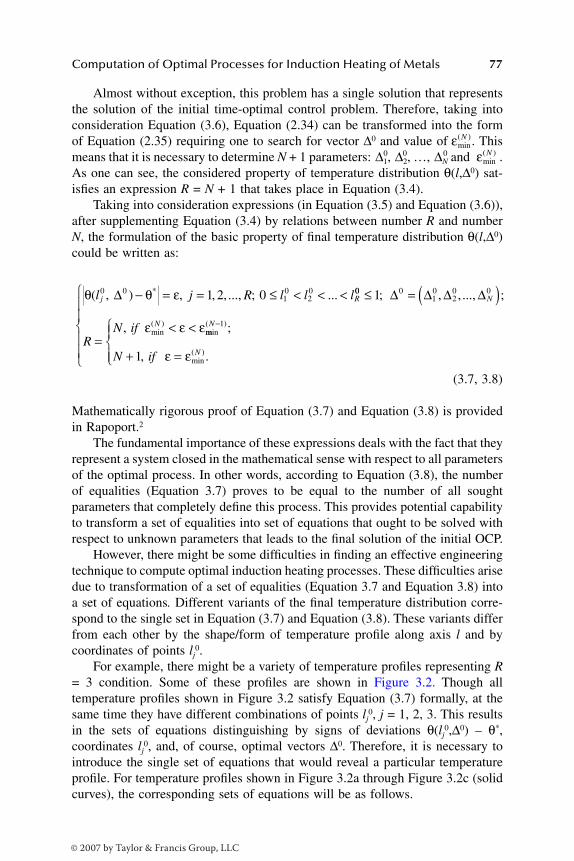
Computation of Optimal Processes for Induction Heating of Metals 77
Almost without exception, this problem has a single solution that representsthe solution of the initial time-optimal control problem. Therefore, taking intoconsideration Equation (3.6), Equation (2.34) can be transformed into the formof Equation (2.35) requiring one to search for vector ∆0 and value of . Thismeans that it is necessary to determine N + 1 parameters: 0∆1,
0∆2, …, 0∆N and .As one can see, the considered property of temperature distribution θ(l,∆0) sat-isfies an expression R = N + 1 that takes place in Equation (3.4).
Taking into consideration expressions (in Equation (3.5) and Equation (3.6)),after supplementing Equation (3.4) by relations between number R and numberN, the formulation of the basic property of final temperature distribution θ(l,∆0)could be written as:
(3.7, 3.8)
Mathematically rigorous proof of Equation (3.7) and Equation (3.8) is providedin Rapoport.2
The fundamental importance of these expressions deals with the fact that theyrepresent a system closed in the mathematical sense with respect to all parametersof the optimal process. In other words, according to Equation (3.8), the numberof equalities (Equation 3.7) proves to be equal to the number of all soughtparameters that completely define this process. This provides potential capabilityto transform a set of equalities into set of equations that ought to be solved withrespect to unknown parameters that leads to the final solution of the initial OCP.
However, there might be some difficulties in finding an effective engineeringtechnique to compute optimal induction heating processes. These difficulties arisedue to transformation of a set of equalities (Equation 3.7 and Equation 3.8) intoa set of equations. Different variants of the final temperature distribution corre-spond to the single set in Equation (3.7) and Equation (3.8). These variants differfrom each other by the shape/form of temperature profile along axis l and bycoordinates of points lj
0.For example, there might be a variety of temperature profiles representing R
= 3 condition. Some of these profiles are shown in Figure 3.2. Though alltemperature profiles shown in Figure 3.2 satisfy Equation (3.7) formally, at thesame time they have different combinations of points lj
0, j = 1, 2, 3. This resultsin the sets of equations distinguishing by signs of deviations θ(lj
0,∆0) – θ*,coordinates lj
0, and, of course, optimal vectors ∆0. Therefore, it is necessary tointroduce the single set of equations that would reveal a particular temperatureprofile. For temperature profiles shown in Figure 3.2a through Figure 3.2c (solidcurves), the corresponding sets of equations will be as follows.
εmin( )N
εmin( )N
θ θ ε( , ) , , , ..., ; ...*l j R l l lj R0 0
10
201 2 0∆ − = = ≤ < < < 00 0
10
20 01≤ = ( )
=< <
; , , ..., ;
, min( )
∆ ∆ ∆ ∆N
N
RN if ε ε εmmin
( )
min( )
;
, .
N
NN if
−
+ =
1
1 ε ε
DK6039_C003.fm Page 77 Monday, June 12, 2006 10:22 AM
© 2007 by Taylor & Francis Group, LLC

78 Optimal Control of Induction Heating Processes
For the profile shown in Figure 3.2a:
For the case in Figure 3.2b:
FIGURE 3.2 Variants of temperature profiles at the end of time-optimal heating processfor R = 3, < ε < .
a
b
c
10
R = 3
R = 3
R = 3
10
10
θ(l, ∆0) − θ∗
θ(l, ∆0) − θ∗
θ(l, ∆0) − θ∗
l10 l
20 l
30
l10 l
20 l
30
l10 l
20 l
30
l
l
l
ε
ε
−ε
ε
−ε
−ε
εmin( )3 εmin
( )2
θ θ ε
θ θ ε
θ θ
( , ) ;
( , ) ;
( , )
*
*
l
l
l
10 0
20 0
30 0
∆
∆
∆
− = −
− = +
− ** .= −
ε
DK6039_C003.fm Page 78 Monday, June 12, 2006 10:22 AM
© 2007 by Taylor & Francis Group, LLC
Computation of Optimal Processes for Induction Heating of Metals 79
For the profile shown in Figure 3.2c:
Even for the same temperature profile θ(l,∆0) – θ* (having greater than Rnumber of extremum points, which are “candidates” on the role of points lj
0),different sets of equations could be written (see dotted curves in Figure 3.2bthrough Figure 3.2c).
The proper choice of a particular temperature distribution θ(l,∆0) allowstransforming Equation (3.7) into a corresponding set of equations. This choicecan only be performed using additional information about a specific of temper-ature distribution (based on physical properties of induction heating processes).The following sections will discuss the ways to accomplish this task.
3.2 EXTENDED DISCUSSION ON PROPERTIES OF FINAL TEMPERATURE DISTRIBUTION FOR TIME-OPTIMAL INDUCTION HEATING PROCESSES
To choose a particular variant of temperature distribution θ(l,∆0), it is necessaryto apply additional information regarding qualitative properties of a temperaturefield that will be obtained at the end of the optimal heating process. The properchoice should be performed according to the required value of ε.
Detailed analysis shows that maximum admissible temperature deviationsθ(lj
0,∆0) – θ* of the final temperature distribution from the required one (seeEquation 3.7) arise with different signs for each pair of successively located pointslj
0.2 It means that these deviation signs are alternating in points lj0, where 0 ≤ l1
0
< l20 < … lR
0 ≤ 1.Taking this feature into consideration, Equation (3.7) and Equation (3.8) can
be rewritten as:
θ θ ε
θ θ ε
θ θ
( , ) ;
( , ) ;
( , )
*
*
l
l
l
10 0
20 0
30 0
∆
∆
∆
− = +
− = +
− ** .= +
ε
θ θ ε
θ θ ε
θ θ
( , ) ;
( , ) ;
( , )
*
*
l
l
l
10 0
20 0
30 0
∆
∆
∆
− = +
− = −
− ** .= −
ε
DK6039_C003.fm Page 79 Monday, June 12, 2006 10:22 AM
© 2007 by Taylor & Francis Group, LLC

80 Optimal Control of Induction Heating Processes
(3.9)
Here, a multiplier coefficient (–1)j provides a sign alternation of temperaturedeviations at points lj
0 that are consecutively located within the interval [0, 1].Coefficient ψ equals to +1 or –1 and provides signs “+” or “–” for temperaturedeviations at each point lj
0.Equation (3.9) significantly restricts the set of admissible temperature curves
θ(l,∆0). For example, Equation (3.7) and Equation (3.8) are true for all temperatureprofiles in Figure 3.2; however, only curves shown in Figure 3.2a meet require-ment (Equation 3.9). The solid curve (Figure 3.2a) corresponds to ψ = –1 and,respectively, the dashed one corresponds to ψ = +1 in Equation (3.9).
The set of points lj0 where equalities (Equation 3.9) hold true are called
Chebyshev alternance1 in approximation theory. In this case, the rule (Equation3.9) represents the fundamental alternance property of the final temperaturedistribution in time-optimal processes of induction heating. This is the reasonwhy the newly proposed optimal control method is called alternance method.
It is important to note that the rule (Equation 3.9) does not yet allow deter-mining the shape/form of curve θ(l,∆0). Additional information with regard to anumber of extremum points on the interval [0,1] is required. Figure 3.3 showsvariants of different temperature profiles θ(l,∆0) for the case of R = 5. All curvessatisfactorily fit condition (3.9). If the curve has a minimal number of extremumpoints, then its form is unambiguously fixed as shown in Figure 3.3a. If thenumber of extremum points exceeds the required minimum (R = 5), then a varietyof curves θ(l,∆0) exists. The difference would also be in locations of points lj
0.Some of these temperature profiles and corresponding points are presented inFigure 3.3b.
Based on physical properties of induction heating temperature fields, it canbe shown that maximum possible number, Mmax, of extremum points for curveθ(l,∆0) is determined according to the following expression2,5:
(3.10)
for model Equation (1.27) through Equation (1.35) with uniform initial temper-ature distribution (Section 2.8), that will be considered further.
Simple physical explanation of Equation (3.10) can be offered. Taking intoconsideration constant maximum power u(ϕ) ≡ Umax, the temperature distributionθ(l,∆1) at the end of induction heating is well known (Figure 3.4). It has two
θ θ ψε( , ) , , , ..., ; ,*l j Rjj0 0 0
10
201 1 2∆ ∆ ∆ ∆− = −( ) = = ,, ..., ,
... ;,
∆R
Rl l l RN if
0
10
20 0
1
0 1
( ) = ±
≤ < < < ≤ =
ψ
εmmin( )
min( )
min( )
,
, .
N N
NN if
< <
+ =
−ε ε
ε ε
1
1
MN if N is even number
N if N is odd numbermax
, ;
, .=
+
1
DK6039_C003.fm Page 80 Monday, June 12, 2006 10:22 AM
© 2007 by Taylor & Francis Group, LLC

Computation of Optimal Processes for Induction Heating of Metals 81
extremum points with minimum and maximum temperatures accordingly: l = le1
= 0 and l = le2, 0 < le2 < 1. The first point corresponds to a boundary condition(Equation 1.31) for l = 0. The second point is formed by negative temperaturegradient on the surface l = 1 due to heat losses, according to the boundarycondition (Equation 1.32) at l = 1. The shape of curve θ(l,∆1) is invariable overthe second bounded control interval under u(ϕ) ≡ 0 (Figure 3.4). During the thirdshort interval, a “peak” of temperature is formed within the billet surface layer.
FIGURE 3.3 Variants of temperature profiles at the end of time-optimal heating processfor R = 5.
FIGURE 3.4 Temperature distribution across workpiece thickness at the end of heatingwith constant maximum power (solid curve) and after soaking stage (dashed curve).
(a)
0
(b)
1
θ(l, ∆0) − θ∗
θ(l, ∆0) − θ∗
l10
l10
l20
l20
l30 l
50
l50l
30
l40
l40
l
1
l
ε
−ε
0
ε
−ε
0 le1 le2 le2 1
l
θ(l, ∆1, ∆2) θ(l, ∆1)
DK6039_C003.fm Page 81 Monday, June 12, 2006 10:22 AM
© 2007 by Taylor & Francis Group, LLC
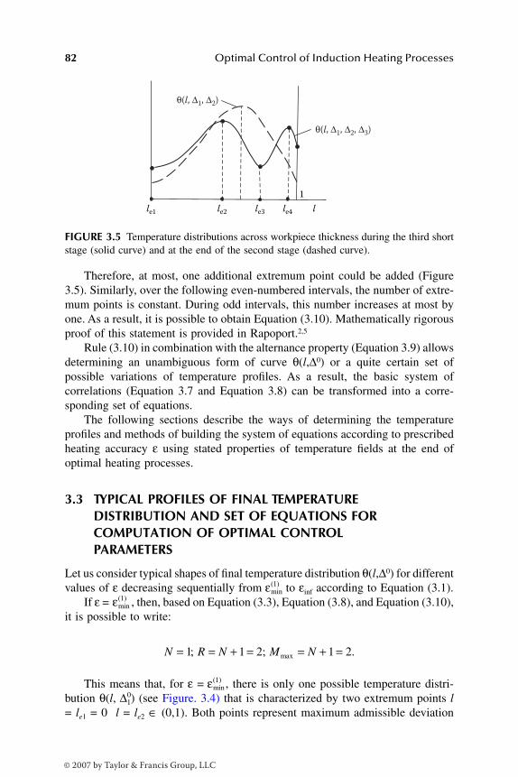
82 Optimal Control of Induction Heating Processes
Therefore, at most, one additional extremum point could be added (Figure3.5). Similarly, over the following even-numbered intervals, the number of extre-mum points is constant. During odd intervals, this number increases at most byone. As a result, it is possible to obtain Equation (3.10). Mathematically rigorousproof of this statement is provided in Rapoport.2,5
Rule (3.10) in combination with the alternance property (Equation 3.9) allowsdetermining an unambiguous form of curve θ(l,∆0) or a quite certain set ofpossible variations of temperature profiles. As a result, the basic system ofcorrelations (Equation 3.7 and Equation 3.8) can be transformed into a corre-sponding set of equations.
The following sections describe the ways of determining the temperatureprofiles and methods of building the system of equations according to prescribedheating accuracy ε using stated properties of temperature fields at the end ofoptimal heating processes.
3.3 TYPICAL PROFILES OF FINAL TEMPERATURE DISTRIBUTION AND SET OF EQUATIONS FOR COMPUTATION OF OPTIMAL CONTROL PARAMETERS
Let us consider typical shapes of final temperature distribution θ(l,∆0) for differentvalues of ε decreasing sequentially from to εinf according to Equation (3.1).
If ε = , then, based on Equation (3.3), Equation (3.8), and Equation (3.10),it is possible to write:
This means that, for ε = , there is only one possible temperature distri-bution θ(l, 0∆1) (see Figure. 3.4) that is characterized by two extremum points l= le1 = 0 l = le2 ∈ (0,1). Both points represent maximum admissible deviation
FIGURE 3.5 Temperature distributions across workpiece thickness during the third shortstage (solid curve) and at the end of the second stage (dashed curve).
1
le1 le2 le3 le4 l
θ(l, ∆1, ∆2)
θ(l, ∆1, ∆2, ∆3)
εmin( )1
εmin( )1
N R N M N= = + = = + =1 1 2 1 2; ; .max
εmin( )1
DK6039_C003.fm Page 82 Monday, June 12, 2006 10:22 AM
© 2007 by Taylor & Francis Group, LLC
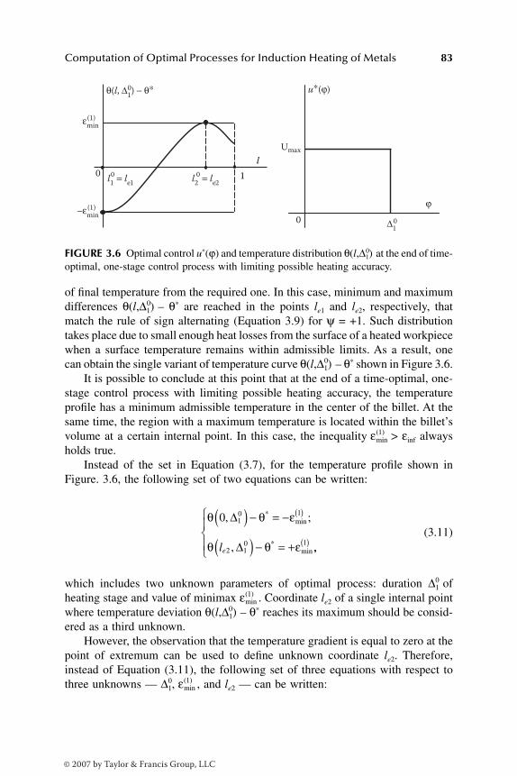
Computation of Optimal Processes for Induction Heating of Metals 83
of final temperature from the required one. In this case, minimum and maximumdifferences θ(l,∆1)
0 – θ* are reached in the points le1 and le2, respectively, thatmatch the rule of sign alternating (Equation 3.9) for ψ = +1. Such distributiontakes place due to small enough heat losses from the surface of a heated workpiecewhen a surface temperature remains within admissible limits. As a result, onecan obtain the single variant of temperature curve θ(l,∆1)
0 – θ* shown in Figure 3.6.It is possible to conclude at this point that at the end of a time-optimal, one-
stage control process with limiting possible heating accuracy, the temperatureprofile has a minimum admissible temperature in the center of the billet. At thesame time, the region with a maximum temperature is located within the billet’svolume at a certain internal point. In this case, the inequality > εinf alwaysholds true.
Instead of the set in Equation (3.7), for the temperature profile shown inFigure. 3.6, the following set of two equations can be written:
(3.11)
which includes two unknown parameters of optimal process: duration ∆10 of
heating stage and value of minimax . Coordinate le2 of a single internal pointwhere temperature deviation θ(l,∆1)
0 – θ* reaches its maximum should be consid-ered as a third unknown.
However, the observation that the temperature gradient is equal to zero at thepoint of extremum can be used to define unknown coordinate le2. Therefore,instead of Equation (3.11), the following set of three equations with respect tothree unknowns — 0∆1, , and le2 — can be written:
FIGURE 3.6 Optimal control u*(ϕ) and temperature distribution θ(l,∆1)0 at the end of time-
optimal, one-stage control process with limiting possible heating accuracy.
1
l
θ(l, ∆10) − θ∗
∆10
u∗(ϕ)
ϕ
l10 = l
e1l20 = l
e2
εmin(1)
−εmin(1)
0
Umax
0
εmin( )1
θ θ ε
θ θ ε
0 10 1
2 10 1
, ;
,
*min
*min
∆
∆
( ) − = −
( ) − = +
( )
( )le ,,
εmin( )1
εmin( )1
DK6039_C003.fm Page 83 Monday, June 12, 2006 10:22 AM
© 2007 by Taylor & Francis Group, LLC
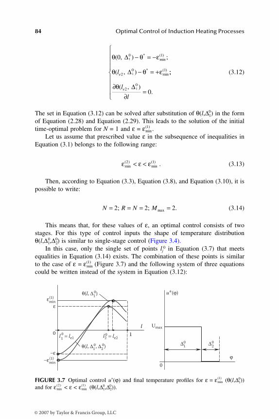
84 Optimal Control of Induction Heating Processes
(3.12)
The set in Equation (3.12) can be solved after substitution of θ(l,∆1)0 in the form
of Equation (2.28) and Equation (2.29). This leads to the solution of the initialtime-optimal problem for N = 1 and ε = .
Let us assume that prescribed value ε in the subsequence of inequalities inEquation (3.1) belongs to the following range:
. (3.13)
Then, according to Equation (3.3), Equation (3.8), and Equation (3.10), it ispossible to write:
(3.14)
This means that, for these values of ε, an optimal control consists of twostages. For this type of control inputs the shape of temperature distributionθ(l,∆1,∆2)
0 is0 similar to single-stage control (Figure 3.4).In this case, only the single set of points lj
0 in Equation (3.7) that meetsequalities in Equation (3.14) exists. The combination of these points is similarto the case of ε = (Figure 3.7) and the following system of three equationscould be written instead of the system in Equation (3.12):
FIGURE 3.7 Optimal control u*(ϕ) and final temperature profiles for ε 0= (θ(l,∆1))and for < ε < 0(θ(l,∆1,∆2)).
0
θ θ ε
θ θ ε
( , ) ;
( , )
*min( )
*min( )
0 1
1
0 1
20 1
∆
∆
− = −
− = +le ;;
( , ).
∂∂
=
θ l
le2
01
0∆
εmin( )1
ε ε εmin( )
min( )2 1< <
N R N M= = = =2 2 2; ; .max
εmin( )1
1
l
θ(l, ∆10)
θ(l, ∆10, ∆
20)
∆10 ∆
20
u∗(ϕ)
ϕ
l10 = le1 l2
0 = le2
εmin(1)
−εmin(1)
0
Umax
0
ε
−ε
εmin( )1
εmin( )2 εmin
( )1
DK6039_C003.fm Page 84 Monday, June 12, 2006 10:22 AM
© 2007 by Taylor & Francis Group, LLC
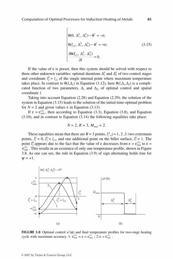
Computation of Optimal Processes for Induction Heating of Metals 85
(3.15)
If the value of ε is preset, then this system should be solved with respect tothree other unknown variables: optimal durations ∆1
0 and ∆20 of two control stages
and coordinate l20 = le2 of the single internal point where maximum temperature
takes place. In contrast to θ(l,∆1) in Equation (3.12), here θ(l,∆1,∆2) is a compli-cated function of two parameters, ∆1 and ∆2, of optimal control and spatialcoordinate l.
Taking into account Equation (2.28) and Equation (2.29), the solution of thesystem in Equation (3.15) leads to the solution of the initial time-optimal problemfor N = 2 and given values ε in Equation (3.13).
If ε = , then according to Equation (3.3), Equation (3.8), and Equation(3.10), and in contrast to Equation (3.14) the following equalities take place:
N = 2, R = 3, Mmax = 2.
These equalities mean that there are R = 3 points, lj0, j = 1, 2 ,3: two extremum
points, l10 = 0, l2
0 = le2, and one additional point on the billet surface, l30 = 1. The
point l30 appears due to the fact that the value of ε decreases from ε > to ε =
. This results in an existence of only one temperature profile, shown in Figure3.8. As one can see, the rule in Equation (3.9) of sign alternating holds true forψ = +1.
FIGURE 3.8 Optimal control u*(ϕ) and final temperature profiles for two-stage heatingcycle with maximum accuracy. 1: < ε < ; 2: ε = .
θ θ ε
θ θ ε
θ
( , , ) ;
( , , ) ;
(
*
*
0 1
1
020
20
20
∆ ∆
∆ ∆
− = −
− = +
∂
le
ll
le2
020
10
, , ).
∆ ∆∂
=
εmin( )2
εmin( )2
εmin( )2
θ(l, Δ10, Δ
20) − θ∗
Δ20 Δ
10l
10 = le1 l
20 = le2
l30
εmin(2)
−εmin(2)
0
0
(a) (b)
2
1
1
Umax
U*(ϕ)ε
−ε
εmin( )2 εmin
( )1 εmin( )2
DK6039_C003.fm Page 85 Monday, June 12, 2006 10:22 AM
© 2007 by Taylor & Francis Group, LLC
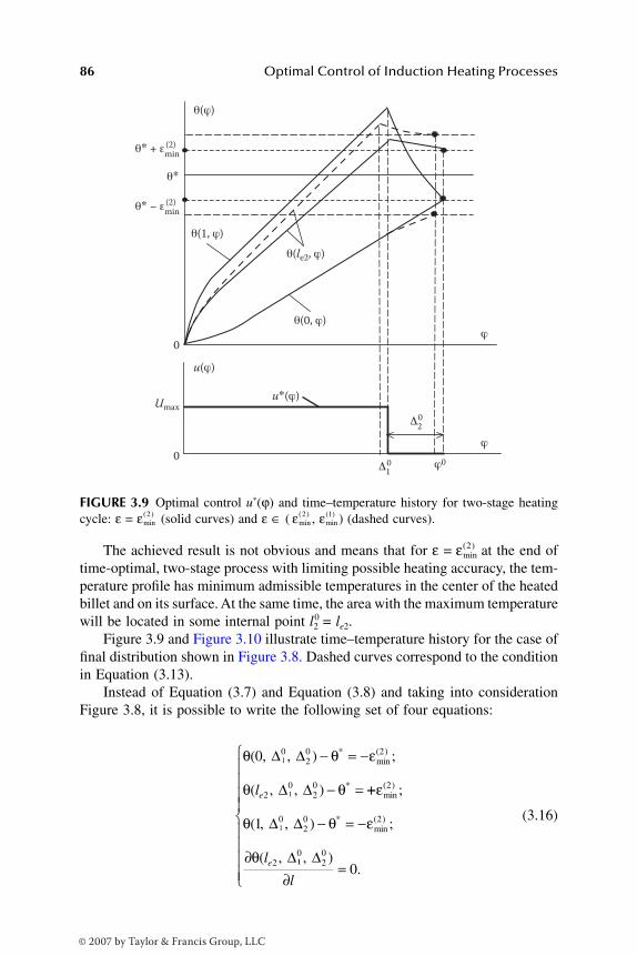
86 Optimal Control of Induction Heating Processes
The achieved result is not obvious and means that for ε = at the end oftime-optimal, two-stage process with limiting possible heating accuracy, the tem-perature profile has minimum admissible temperatures in the center of the heatedbillet and on its surface. At the same time, the area with the maximum temperaturewill be located in some internal point l2
0 = le2.Figure 3.9 and Figure 3.10 illustrate time–temperature history for the case of
final distribution shown in Figure 3.8. Dashed curves correspond to the conditionin Equation (3.13).
Instead of Equation (3.7) and Equation (3.8) and taking into considerationFigure 3.8, it is possible to write the following set of four equations:
(3.16)
FIGURE 3.9 Optimal control u*(ϕ) and time–temperature history for two-stage heatingcycle: ε = (solid curves) and ε ∈ ( , ) (dashed curves).
θ(ϕ)
u(ϕ)
u∗(ϕ)
θ(1, ϕ)
θ(0, ϕ)
θ(le2, ϕ)
Δ20
Δ10
θ∗ + εmin(2)
θ∗ − εmin(2)
0
0
Umax
θ∗
ϕ
ϕ
ϕ0
εmin( )2 εmin
( )2 εmin( )1
εmin( )2
θ θ ε
θ θ
( , , ) ;
( , , )
*min( )
*
0 1
1
020 2
20
20
∆ ∆
∆ ∆
− = −
− =le ++
− = −
∂
ε
θ θ ε
θ
min( )
*min( )
;
( , , ) ;
( ,
2
020 2
2
1 1∆ ∆
∆le 110
20
0, )
.∆
∂=
l
DK6039_C003.fm Page 86 Monday, June 12, 2006 10:22 AM
© 2007 by Taylor & Francis Group, LLC

Computation of Optimal Processes for Induction Heating of Metals 87
As one can see, this set of equations includes four unknown variables: 0∆1,0∆2,
, and le2.Therefore, for any value of ε: ≤ ε ≤ , the shapes of temperature curve
θ(l,∆0) (Figure 3.11) and appropriate computational sets of Equation (3.12),Equation (3.15), and Equation (3.16) are well determined. After substitution ofθ(l,∆0) in the form of Equation (2.28) and Equation (2.29) into equation sets andusing known numerical methods, these sets can be solved with respect to allsought parameters. Obtained optimal value ∆0 represents the solution of the initialtime-optimal problem in the form of Equation (2.34).
It should be emphasized that an ability to define minimum attainable minimaxvalues and is of special interest. This follows from solution of the com-putational systems where values and are considered as unknown para-meters of an optimal control process.
If the process demands better heating accuracy, i.e., the prescribed deviationε should be less than , then values of ε will belong to the following range:
, (3.17)
and the problem will be significantly complicated.It is feasible to determine only the set of possible variants of temperature
profiles θ(l,∆0). Every variant corresponds only to certain, but a priori unknown,initial data. It primarily depends on the value of heat losses during the heatingprocess. Generally speaking, it is not possible in advance to choose a single
FIGURE 3.10 Temperature distribution across workpiece thickness/radius at differenttime points of two-stage optimal heating cycle: ε = (solid curves) and ε ∈ ( , )(dashed curve).
1
l
ϕ = Δ10 + Δ
20
ϕ = Δ10
ϕ < Δ10
le2
θ(l, ϕ)
θ∗ + εmin(2)
θ∗ − εmin(2)
0
θ∗
εmin( )2 εmin
( )2 εmin( )1
εmin( )2
εmin( )2 εmin
( )1
εmin( )1 εmin
( )2
εmin( )1 εmin
( )2
εmin( )2
ε ε εmin( )
min( )3 2≤ <
DK6039_C003.fm Page 87 Monday, June 12, 2006 10:22 AM
© 2007 by Taylor & Francis Group, LLC
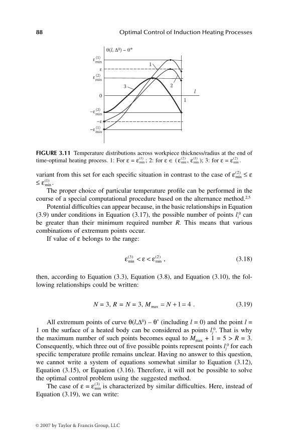
88 Optimal Control of Induction Heating Processes
variant from this set for each specific situation in contrast to the case of ≤ ε≤ .
The proper choice of particular temperature profile can be performed in thecourse of a special computational procedure based on the alternance method.2,5
Potential difficulties can appear because, in the basic relationships in Equation(3.9) under conditions in Equation (3.17), the possible number of points li
0 canbe greater than their minimum required number R. This means that variouscombinations of extremum points occur.
If value of ε belongs to the range:
, (3.18)
then, according to Equation (3.3), Equation (3.8), and Equation (3.10), the fol-lowing relationships could be written:
N = 3, R = N = 3, . (3.19)
All extremum points of curve θ(l,∆0) – θ* (including l = 0) and the point l =1 on the surface of a heated body can be considered as points lj
0. That is whythe maximum number of such points becomes equal to Mmax + 1 = 5 > R = 3.Consequently, which three out of five possible points represent points lj
0 for eachspecific temperature profile remains unclear. Having no answer to this question,we cannot write a system of equations somewhat similar to Equation (3.12),Equation (3.15), or Equation (3.16). Therefore, it will not be possible to solvethe optimal control problem using the suggested method.
The case of ε = is characterized by similar difficulties. Here, instead ofEquation (3.19), we can write:
FIGURE 3.11 Temperature distributions across workpiece thickness/radius at the end oftime-optimal heating process. 1: For ε = ; 2: for ε ∈ ( , ); 3: for ε = .
1
l 2
1
3
θ(l, Δ0) − θ∗
εmin(1)
εmin(2)
ε
−εmin(2)
−εmin(1)
−ε
0
εmin( )1 εmin
( )2 εmin( )1 εmin
( )2
εmin( )2
εmin( )1
ε ε εmin( )
min( )3 2< <
M Nmax = + =1 4
εmin( )3
DK6039_C003.fm Page 88 Monday, June 12, 2006 10:22 AM
© 2007 by Taylor & Francis Group, LLC
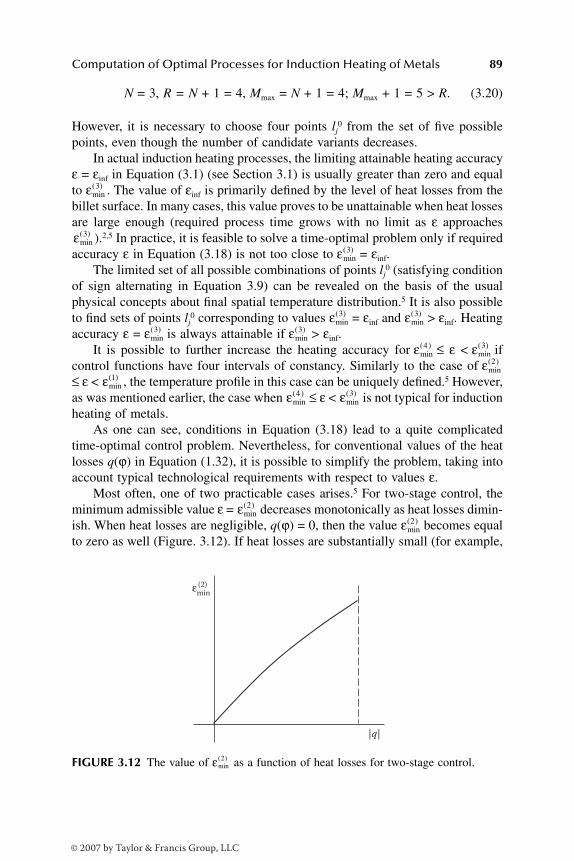
Computation of Optimal Processes for Induction Heating of Metals 89
N = 3, R = N + 1 = 4, Mmax = N + 1 = 4; Mmax + 1 = 5 > R. (3.20)
However, it is necessary to choose four points lj0 from the set of five possible
points, even though the number of candidate variants decreases.In actual induction heating processes, the limiting attainable heating accuracy
ε = εinf in Equation (3.1) (see Section 3.1) is usually greater than zero and equalto . The value of εinf is primarily defined by the level of heat losses from thebillet surface. In many cases, this value proves to be unattainable when heat lossesare large enough (required process time grows with no limit as ε approaches
).2,5 In practice, it is feasible to solve a time-optimal problem only if requiredaccuracy ε in Equation (3.18) is not too close to = εinf.
The limited set of all possible combinations of points lj0 (satisfying condition
of sign alternating in Equation 3.9) can be revealed on the basis of the usualphysical concepts about final spatial temperature distribution.5 It is also possibleto find sets of points lj
0 corresponding to values = εinf and > εinf. Heatingaccuracy ε = is always attainable if > εinf.
It is possible to further increase the heating accuracy for ≤ ε < ifcontrol functions have four intervals of constancy. Similarly to the case of≤ ε < , the temperature profile in this case can be uniquely defined.5 However,as was mentioned earlier, the case when ≤ ε < is not typical for inductionheating of metals.
As one can see, conditions in Equation (3.18) lead to a quite complicatedtime-optimal control problem. Nevertheless, for conventional values of the heatlosses q(ϕ) in Equation (1.32), it is possible to simplify the problem, taking intoaccount typical technological requirements with respect to values ε.
Most often, one of two practicable cases arises.5 For two-stage control, theminimum admissible value ε = decreases monotonically as heat losses dimin-ish. When heat losses are negligible, q(ϕ) = 0, then the value becomes equalto zero as well (Figure. 3.12). If heat losses are substantially small (for example,
FIGURE 3.12 The value of as a function of heat losses for two-stage control.
εmin( )3
εmin( )3
εmin( )3
εmin( )3 εmin
( )3
εmin( )3 εmin
( )3
εmin( )4 εmin
( )3
εmin( )2
εmin( )1
εmin( )4 εmin
( )3
εmin( )2
εmin( )2
εmin(2)
|q|
εmin( )2
DK6039_C003.fm Page 89 Monday, June 12, 2006 10:22 AM
© 2007 by Taylor & Francis Group, LLC

90 Optimal Control of Induction Heating Processes
during heating of aluminum alloy ingots prior to hot forming), then the valuebecomes appreciably small and required values ε meet inequalities ≤
ε < . Therefore, a single- or two-stage control can provide required heatingaccuracy in this case and a complicated control algorithm under N ≥ 3 is notrequired.
If surface heat losses are appreciably large (for example, during heating oftitanium and steel alloy ingots before hot forming), then, quite the contrary, heatlosses increase up to the level when inequality ε < becomes true. Here,minimax coincides with εinf > 0 and becomes unattainable. In this case, it isnecessary to solve the time-optimal problem for the control functions with threeintervals under conditions in Equation (3.18).
However, a high level of heat losses allows one to define unambiguously thesimplest possible variant of curve θ(l,∆0) – θ*.5 This variant differs by the factthat, due to the negative temperature gradient in billet surface layers (see Figure3.5), the temperature “spike” does not appear during the third interval. In otherwords, during the third interval, due to shortage of heating power and/or due torelatively short heating duration, a final temperature distribution (typical for atwo-stage control) is not distorted. In this case, the number of extremum pointsis equal to two (dotted curve in Figure 3.5) and becomes less than Mmax = 4.
As a result, the shape of curve 0θ(l,∆1,∆2,∆3)0 –0 θ* for < ε < replicates
the shape of curve 0θ(l,∆1,∆2)0 – θ* for ε = (Figure 3.13).
If a prescribed value of ε satisfies the following condition, ε < , then theappropriate set of four equations can be written as:
(3.21)
This set of equations should be solved similarly to those in Equation (3.16)with respect to sought optimal durations, ∆1,
0 ∆2,0 ∆3,
0 of three control stages andcoordinate, le2, of the point of maximum final temperature. Here, θ(l,∆1,∆2,∆3) isa complicated function of three parameters, ∆1, ∆2, ∆3, of optimal control andspatial coordinate l.
3.4 COMPUTATIONAL TECHNIQUE FOR TIME-OPTIMAL CONTROL PROCESSES
As has been shown in Section 3.3, for the most practical cases, the set of equationsin Equation (3.12), Equation (3.15), Equation (3.16), or Equation (3.21) shouldbe solved with respect to parameters of a time-optimal induction heating process.
εmin( )2 εmin
( )2
εmin( )1
εmin( )2
εmin( )3
εmin( )3 εmin
( )2
εmin( )2
εmin( )2
θ θ ε
θ θ
( , , , ) ;
( , , , )
*0 1
1
020
30
20
20
30
∆ ∆ ∆
∆ ∆ ∆
− = −
−le**
*
;
( , , , ) ;
( , ,
= +
− = −
∂
ε
θ θ ε
θ
1 1
1
020
30
20
20
∆ ∆ ∆
∆ ∆le ,, ).
∆30
0∂
=
l
DK6039_C003.fm Page 90 Monday, June 12, 2006 10:22 AM
© 2007 by Taylor & Francis Group, LLC

Computation of Optimal Processes for Induction Heating of Metals 91
For a particular application, the appropriate set of equations should be chosenand solved. The choice of set of equations can only be made if the location ofvalue ε in the subsequence of inequalities (Equation 3.1) is known. This locationis defined by Equation (3.3).
There are two quite different possible variants of value assignment forrequired accuracy ε:
1. The fixed numerical value of ε can be prescribed a priori according tospecific technological requirements. (For example, it could be neces-sary that the final temperature in any point of billet would not deviategreater than 25°C from a desired temperature distribution.)
2. It can be assumed that value ε is equal to one of the minimax valuesin Equation (3.1). This means that, at the end of the optimal heatingprocess, the deviation of final temperature distribution from therequired one should be as small as possible for the chosen class ofcontrol inputs.
In both cases, the minimax values in Equation (3.1) are not defined a priori.Under given conditions, the following simple computational procedure is
suggested for determining algorithms of optimal control for induction heatingprocesses.
At the beginning, the sets of equations in Equation (3.12) and Equation (3.16)can be solved assuming that required accuracy ε = and ε = in Equation(2.34). This leads to definition of minimax values and as well as corre-sponding vectors ∆0( ) and ∆0( ) determining optimal control intervals.Therefore, the considered problem is already solved at this stage for case 2.
The optimal control problem is also solved for case 1 if the prescribednumerical value of ε coincides with one of the obtained numerical values ofminimaxes or . Otherwise, it is necessary to compare the prescribednumerical value of ε with obtained values of and . If this value of ε
FIGURE 3.13 Final temperature profiles (a) and optimal control u*(ϕ) (b). 1: For ε ∈( , ) at high levels of heat losses; 2: for ε = .
1
l
u∗1
2
a b
Umax
0 ϕ
Δ30Δ1
0 Δ20
le2
θ(l, Δ0) − θ∗
εmin(2)
εmin(3) ε
−εmin(3)
−εmin(2)
−ε
0
εmin( )3 εmin
( )2 εmin( )2
εmin( )k
εmin( )1 εmin
( )2
εmin( )1 εmin
( )2
εmin( )1 εmin
( )2
εmin( )1 εmin
( )2
εmin( )1 εmin
( )2
DK6039_C003.fm Page 91 Monday, June 12, 2006 10:22 AM
© 2007 by Taylor & Francis Group, LLC
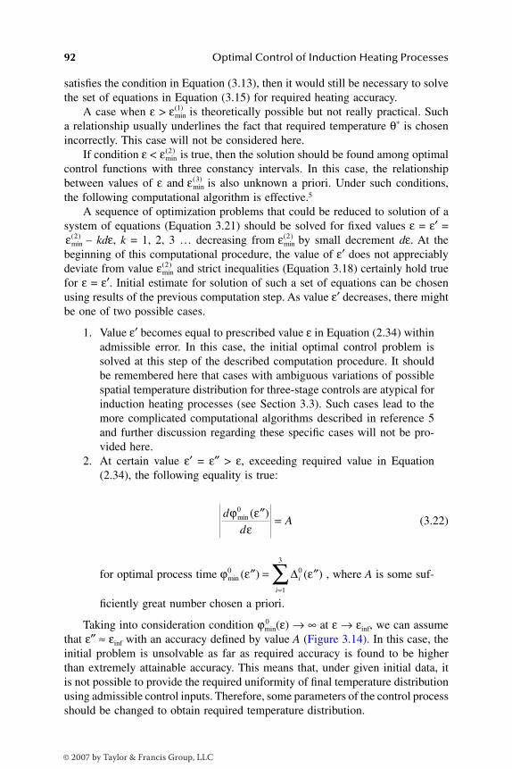
92 Optimal Control of Induction Heating Processes
satisfies the condition in Equation (3.13), then it would still be necessary to solvethe set of equations in Equation (3.15) for required heating accuracy.
A case when ε > is theoretically possible but not really practical. Sucha relationship usually underlines the fact that required temperature θ* is chosenincorrectly. This case will not be considered here.
If condition ε < is true, then the solution should be found among optimalcontrol functions with three constancy intervals. In this case, the relationshipbetween values of ε and is also unknown a priori. Under such conditions,the following computational algorithm is effective.5
A sequence of optimization problems that could be reduced to solution of asystem of equations (Equation 3.21) should be solved for fixed values ε = ε′ =
– kdε, k = 1, 2, 3 … decreasing from by small decrement dε. At thebeginning of this computational procedure, the value of ε′ does not appreciablydeviate from value and strict inequalities (Equation 3.18) certainly hold truefor ε = ε′. Initial estimate for solution of such a set of equations can be chosenusing results of the previous computation step. As value ε′ decreases, there mightbe one of two possible cases.
1. Value ε′ becomes equal to prescribed value ε in Equation (2.34) withinadmissible error. In this case, the initial optimal control problem issolved at this step of the described computation procedure. It shouldbe remembered here that cases with ambiguous variations of possiblespatial temperature distribution for three-stage controls are atypical forinduction heating processes (see Section 3.3). Such cases lead to themore complicated computational algorithms described in reference 5and further discussion regarding these specific cases will not be pro-vided here.
2. At certain value ε′ = ε″ > ε, exceeding required value in Equation(2.34), the following equality is true:
(3.22)
for optimal process time , where A is some suf-
ficiently great number chosen a priori.
Taking into consideration condition 0ϕmin(ε) → ∞ at ε → εinf, we can assumethat ε″ ≈ εinf with an accuracy defined by value A (Figure 3.14). In this case, theinitial problem is unsolvable as far as required accuracy is found to be higherthan extremely attainable accuracy. This means that, under given initial data, itis not possible to provide the required uniformity of final temperature distributionusing admissible control inputs. Therefore, some parameters of the control processshould be changed to obtain required temperature distribution.
εmin( )1
εmin( )2
εmin( )3
εmin( )2 εmin
( )2
εmin( )2
d
dA
ϕ εε
min ( )0 ′′ =
ϕ ε εmin ( ) ( )0 0
1
3
′′ = ′′=∑∆i
i
DK6039_C003.fm Page 92 Monday, June 12, 2006 10:22 AM
© 2007 by Taylor & Francis Group, LLC
Computation of Optimal Processes for Induction Heating of Metals 93
If an induction heater has improved thermal insulation (refractory) that allowsdrastic reduction of surface heat losses leading to further reduction of the valueεinf and inequality εinf < ε in Equation (2.34) becomes true, then an original optimalcontrol problem will be reduced to case 1. A similar effect can be obtained usinghigher frequency heating or increased power of internal heat sources.
All sets of equations can be solved by typical numerical methods, includingthe well-known iteration algorithm.6 According to this algorithm, each system isdivided into two blocks. The first block includes one equation, which representsthe equality of temperature gradient in the point le2 to zero (last equation insystems in Equation 3.12, Equation 3.15, Equation 3.16, and Equation 3.21). Thesecond block includes all remaining equations of the set.
For each kth approximation ∆[k] of sought vector of parameters ∆0, the appro-priate approximation of coordinate l2
0 = le2 can be determined as a solution ofthe first equation that forces temperature gradients to be equal to zeroes:
. (3.23)
The next approximation, ∆[k+1], is defined as a solution of the set of equationsof the second block, where it is assumed that le2 = . For example, in the caseof Equation (3.16), this block consists of three equations:
(3.24)
FIGURE 3.14 Minimum heating time as a function of heating accuracy.
ϕmin0
εmin(2) ε
min = εinf
(3)
εεʹεʺ
lek2
[ ]
∂ ( )∂
= =θ l
lk
ek k2
0 0 1 2[ ] [ ],
, , , , ...∆
lek2
[ ]
θ θ ε
θ
( , , ) ;
( ,
[ ] [ ] *min( )
[ ]
0 11
21 2
2
∆ ∆
∆
k k
ekl
+ + − = −
11
1
12
1 2
121
[ ] [ ] *min( )
[ ]
, ) ;
( , ,
k k
k
+ +
+
− = +∆
∆ ∆
θ ε
θ [[ ] *min( )) .k+ − = −
1 2θ ε
DK6039_C003.fm Page 93 Monday, June 12, 2006 10:22 AM
© 2007 by Taylor & Francis Group, LLC
94 Optimal Control of Induction Heating Processes
After solving this set of equations, one can obtain ∆1[k+1], ∆2
[k+1], and on each(k + 1)th step of the computational procedure (k = 0, 1, 2, ...).
The following set of three equations can be written regarding Equation (3.21):
(3.25)
Here, ∆[k+1],1
∆[k+1],2 and ∆[k+1]3 are unknown parameters; however, the value of ε is
prescribed. The sets of Equation (3.12) and Equation (3.15) are solved in a similarmanner.
The described iteration procedure is repeated for predetermined initial valueof ∆[0] until value ∆[r] coincides satisfactorily with ∆[r+1] on some step under k =r. Convergence of this procedure is typically guaranteed only if the initial valueof ∆[0] is chosen properly. Values ∆[0] can be determined with fair accuracy usingthe following algorithms.
If ε = , then the value ∆[0] = ∆1[0] can be found as a duration of the heating
interval with constant power u(ϕ) ≡ Umax that would be necessary to provide billetfinal average temperature equal to required average temperature θ*. For ε = ,it is possible to assume that duration ∆1
[0] of the first interval of two-stage processcontrol is equal to the value ∆1
[0] ( ) ≅ ∆1[0] ( ) for one-stage control. The
second time interval can be calculated approximately as5:
, (3.26)
where q0 is time-average value of heat losses in Equation (1.32), which can becalculated, according to Equation (1.34); µ1 is the first root of Equation (1.43).All other denotations are discussed in Chapter 1.
For ε = , there is a simple exponential relationship between the value∆2
[0] and value of heat losses. As shown in Rapoport,5 the following expressiontakes place:
, (3.27)
i.e., the coordinate of point of maximum temperature does not depend on optimalprocess parameters.
The values 1(∆[0],∆[0])2 are defined as a solution of the set of equations inEquation (3.16). As a rule, these values can be used as initial approximation forsolving the set of equations in Equation (3.15). In this case, values ε shouldoccupy the following range: < ε < .
εmin( )2
θ θ ε
θ
( , , , ) ;
(
[ ] [ ] [ ] *
[ ]
0 11
21
31
2
∆ ∆ ∆k k k
ekl
+ + + − = −
,, , , ) ;
( ,
[ ] [ ] [ ] *
[
∆ ∆ ∆
∆
1
1
12
13
1
11
k k k
k
+ + +
+
− = +θ ε
θ ]] [ ] [ ] *, , ) .∆ ∆21
31k k+ + − = −
θ ε
εmin( )1
εmin( )2
εmin( )1 εmin
( )2
∆20
12
12 2
1 0
1 1
14 1
[ ] ln( )
( )( ( ))≅ −
−µµ µ
ξ µK q
W K
εmin( )2
le20 2
3[ ] ≈
εmin( )2 εmin
( )1
DK6039_C003.fm Page 94 Monday, June 12, 2006 10:22 AM
© 2007 by Taylor & Francis Group, LLC

Computation of Optimal Processes for Induction Heating of Metals 95
Every set of equations (Equation 3.21) is solved for decreasing sequence ofvalues ε = ε′. These values are obtained by utilizing a three-stage control. Initialestimates ∆[0] used for solution of such systems can be chosen by applying resultsobtained from a previous step of computation. During the first step of thiscomputational procedure, the values 1∆[0]( ), 2∆[0]( ) are used as initial esti-mates of 1∆[0], ∆[0]
2 for ε = ε′ = – dε.Unknown values of minimaxes and could be excluded from calcula-
tional sets of equations in Equation (3.12) and Equation (3.16), replacing initialequations by their sums or differences. This allows reducing the system dimen-sion, decreasing the number of sought unknowns, and simplifying calculations.Therefore, by combining the first two equations in Equation (3.12), it is possibleto obtain the following set of two equations with respect to two unknowns —∆1
0 and le2:
(3.28)
Combining the first equation with the second and the second equation withthe third in Equation (3.16), it is possible to obtain the set of three equations withrespect to three unknowns — 0∆1, ∆2,
0 and le2 (instead of four equations in Equation3.16):
(3.29)
Minimax values are calculated from appropriate equalities in Equation (3.12)and Equation (3.16) after solving sets of equations in Equation (3.28) and Equa-tion (3.29). Therefore,
or
and
; , or .
εmin( )2 εmin
( )2
εmin( )2
εmin( )1 εmin
( )2
θ θ θ
θ
( , ) ( , ) ;
( , ).
*0 2 0
0
1 1
1
02
0
20
∆ ∆
∆
+ − =
∂∂
=
l
l
l
e
e
θ θ θ
θ
( , , ) ( , , ) ;
( ,
*0 2 01 1
1
020
20
20
20
∆ ∆ ∆ ∆
∆
+ − =l
l
e
e ,, ) ( , , ) ;
( , , )
*∆ ∆ ∆
∆ ∆
20 0
20
20
20
1 2 01
1
+ − =
∂∂
θ θ
θ l
le ==
0.
ε θ θmin( ) *( , )1
201= −le ∆ ε θ θmin
( ) * ( , )1 00 1= − ∆
ε θ θmin( ) *( , , )2
20 01 2= −le ∆ ∆ ε θ θmin
( ) * ( , , )2 0 00 1 2= − ∆ ∆ ε θ θmin( ) * ( , , )2 0 01 1 2= − ∆ ∆
DK6039_C003.fm Page 95 Monday, June 12, 2006 10:22 AM
© 2007 by Taylor & Francis Group, LLC

96 Optimal Control of Induction Heating Processes
Using the previously mentioned linear dependence of a set of equations fromε, it is possible to significantly simplify the computational procedure for three-stage optimal control when ε < . For this purpose, it is necessary to “swapthe roles” of values ε and ∆3
0 in Equation (3.21). It should be assumed that valueof ε is unknown instead of value ∆3
0 (which is considered as fixed third constancyinterval of optimal control function). Then, this new unknown can be excludedusing linear combinations of equations in Equation (3.21) like Equation (3.28)and Equation (3.29). As a result, the set in Equation (3.21) can be rewritten withrespect to three unknowns 0∆1, ∆2
0 le2 for preassigned value 0∆3:
(3.30)
Computation results5 show that the value ∆30 decreases with ε on the interval
[ ; ] until ∆30 = 0 at ε = (Figure 3.15). In this case, instead of solving
a sequence of sets of four equations (Equation 3.21) using small step dε, it wouldbe possible to transform an initial optimal control problem into a much simplerproblem that would require solving the sequence of sets of equations in Equation(3.30) for sequence of values ∆3
0 increasing from zero using appreciably smallstep d∆3.
0 The value ε can be calculated for the appropriate step from any of thefirst three equations in Equation (3.21). Obtained values of ε diminish withincreasing sequence of prescribed values of ∆3.
0 Here, the approach similar tosolution of the set in Equation (3.21) is used.
FIGURE 3.15 Duration of the third stage of heating cycle as a function of required heatingaccuracy.
εmin( )2
θ θ θ
θ
( , , , ) ( , , , ) ;*0 2 01 10
20
30
20
20
30∆ ∆ ∆ ∆ ∆ ∆+ − =le
(( , , , ) ( , , , ) ;*le20
20
30 0
20
30
1 11 2 0∆ ∆ ∆ ∆ ∆ ∆+ − =
∂
θ θ
θθ( , , , ).
l
le2
020
30
10
∆ ∆ ∆∂
=
εmin( )3 εmin
( )2 εmin( )2
∆30
εmin(2)ε
min(3)
ε
DK6039_C003.fm Page 96 Monday, June 12, 2006 10:22 AM
© 2007 by Taylor & Francis Group, LLC

Computation of Optimal Processes for Induction Heating of Metals 97
The finite number of terms of series in Equation (2.29) is always used ingoverning equation sets. An important question arises at this point with regardto an accuracy of obtained results that depends on computational accuracy ofinfinite series.
Let us assume that is the exact solution of a set of equations obtained forfinite number S < ∞ of the series terms in Equation (2.29). Let us also assumethat an error of temperature field computation, δ, is caused by truncation. Then,instead of basic equations in Equation (3.7), the following expressions hold trueat points lj
0:
. (3.31)
It can be shown5 that, if the value δ is appreciably small, then the variationof the exact solution ∆0 of the set of equations that is obtained with all terms ofthe series in Equation (2.29) would differ from for the value that is no greaterthan 2δ:
. (3.32)
For convergent Fourier series in Equation (2.29), δ → 0 under S → ∞.Therefore, converges to ∆0 at S → ∞ according to Equation (3.32). Experienceof practical computation shows5 that for S ≥ 10 … 20, a quite high accuracy isachieved for computation of temperature distribution. Maximum error does notexceed 0.5%. Therefore, ∆0 can be calculated with the same accuracy in allpracticable cases. Without considerable difficulties, the required number of seriesterms in the set of equations can be utilized using modern computers.
3.5 APPLICATION OF THE SUGGESTED METHOD TO MODEL PROBLEMS BASED ON TYPICAL COST FUNCTIONS
An engineering technique for solving general time-optimal control problems forinduction heating of metals has been discussed in previous chapters. It has beenshown that, with respect to the mathematical model (Equation 1.27 throughEquation 1.35), time-optimal control problems can be reduced to the nonstandardproblem of mathematical programming (Equation 2.34). Naturally, one might beinterested whether it is possible to use the suggested method for other types ofdifferent typical optimization problems discussed in Section 2.9.
First of all, let us notice that the previously described computational techniqueremains unchanged as applied to the optimization problem (Equation 2.33) forsteady-state continuous heating. Such heating processes are described by the samemathematical model (Equation 1.27 through Equation 1.35) with substitution ofthe variable (Equation 2.6). However, lengths of inductor sections, ∆i,* should be
∆0
θ θ ε δ( , ) , , , ...,*l j Rj0 0 1 2∆ − − ≤ =
∆0
∆ ∆i i for all i N0 0 2 1− ≤ = δ ,
∆0
DK6039_C003.fm Page 97 Monday, June 12, 2006 10:22 AM
© 2007 by Taylor & Francis Group, LLC
98 Optimal Control of Induction Heating Processes
considered as sought parameters instead of time intervals, ∆i , of optimal controlfor static induction heating. Moreover, all properties of spatial temperature dis-tributions at the end of optimal static heating relate to temperature distributionsover billet cross-section at the exit of a continuous heater. Therefore, all expres-sions for θ(l,∆) in the sets of equations in Equation (3.12), Equation (3.15),Equation (3.16), and Equation (3.21) should be changed for θ(l,∆*/V) by simplesubstitution .
The method can be applied to the optimization problems for heating whenmaximum accuracy is required. Such problems are formulated using Equation(2.35), Equation (2.36), and Equation (2.37). As shown in Section 2.9.1, they canbe reduced to the appropriate time-optimal problems under the absence of exces-sive heating time.
A multicoil continuous heater consists of a number of individual coils. Insteadof using the lengths of coils of the induction heater, a voltage applied to eachcoil can be used as control input in Equation (2.38). In this case, expression θ(l,U)should be used as a representation of radial temperature profile at the exit end ofthe multicoil induction heater instead of θ(l,∆*/V) in Equation (2.37). Neverthe-less, as investigations and computer modeling evaluation show, all properties offinal temperature distribution, governing sets of equations, and computationalprocedures described in Section 3.1 through Section 3.4 are kept identical to thetime-optimal problem for static heating processes. It will only be required tosubstitute analytical expressions for θ(l,U0) instead of θ(l,∆0) (see Section 2.9.1)in governing sets of equations. In addition, unknowns 0∆1,
0∆2, …, ∆N0 should be
changed to U1,0 U2,
0 …, 0UN.For the problem described by Equation (2.42) that represents optimization of
minimum power consumption during induction heating, the described methodwill have various forms (see Section 2.9.2). In this case, the general optimalcontrol algorithm is the same and time lengths of alternating intervals of heatingand soaking remain unknown. Therefore, the vector ∆ should be defined. Inaddition, basic properties in Equation (3.7) and Equation (3.8) remain valid forthe temperature distribution at the end of the optimal process. However, alternanceproperty (Equation 3.9) is violated for such distribution, and the rule in Equation(3.3) will not be appropriate for the definition of number of constancy intervalsN.2,5
Therefore, if energy saving is a goal of the optimal control algorithm, thenit will not be possible to write the set of equations by simply applying conclusionsregarding temperature profile θ(l,∆0) (appropriate validation was made in Section3.3). The difference between minimum power consuming and time-optimal con-trol algorithms (assuming similar required heating accuracy) has been discussedin Section 2.9.2. Thus, in a case when ε = , the time-optimal control algorithmwould not be optimal for power cost function. Energy consumption can becalculated as:
IE = Umax∆1. (3.33)
∆ ∆i i V i N= =* / , ,1
εmin( )1
DK6039_C003.fm Page 98 Monday, June 12, 2006 10:22 AM
© 2007 by Taylor & Francis Group, LLC

Computation of Optimal Processes for Induction Heating of Metals 99
It is possible to reduce IE by decreasing the first (and in this case single)control interval in comparison with duration of time-optimal control. To obtainrequired heating accuracy, it is necessary to apply the second interval that repre-sents temperature soaking. During soaking stage, there would be no energyapplied to induction coil: u(ϕ) ≡ 0. There is a unique correlation between thevalue of and maximum value ∆2. If that value would be exceeded, then theinverse effect would take place: temperature nonuniformity will worsen due tosurface heat losses. This situation can take place because, during the soakingstage, the surface temperature falls lower than minimum admissible level. In thisparticular case, the following expressions could be written for N = 2 accordingto basic rule R = N in Equation (3.7) and Equation (3.10):
.
As one can see, if ε = and N = 2, there is only one possible finaltemperature distribution for a minimum power consuming process. Figure 3.16shows this temperature profile. As this takes place, because additional energy isconsumed during following odd intervals, a two-stage control function would beoptimal with respect to criterion IE.
The control that optimizes energy consumption of an induction heater appre-ciably differs from time-optimal control for ε = . A minimum power con-sumption process consists of two stages (compared to a single-stage control fora time-optimal problem). Therefore, the condition in (Equation 3.3) would notbe valid in this case. The final temperature distribution is characterized by reach-ing minimum admissible temperatures in the billet center and on the billet surface.The final maximum temperature does not reach its utmost admissible value (seeFigure 3.16). Thus, the alternance condition in Equation (3.9) that has beenestablished for time-optimal processes is violated.
It is proper to remember at this point that, at the end of a time-optimal process,the maximum temperature deviations of final temperature from the required oneare reached with different signs at the points l = 0 and l = le2 (see Figure 3.6).
FIGURE 3.16 Temperature profile at the end of minimum power consumption processfor ε = .
εmin( )1
R N for M N= = = > = =2 21 2ε ε εmin( )
min( )
max;
εmin( )1
εmin( )1
1
θ(l, ∆0) − θ∗ε
min(1)
−εmin(1)
0
l
−
εmin( )1
DK6039_C003.fm Page 99 Monday, June 12, 2006 10:22 AM
© 2007 by Taylor & Francis Group, LLC

100 Optimal Control of Induction Heating Processes
As a result, according to the temperature curve in Figure 3.16, for ε = ,the governing set of equations can be written as:
(3.34)
Here, time intervals of power cost optimal control are denoted as and incontrast to parameters of the time-optimal process.
The given set of two equations can be solved with respect to twounknowns, , under prescribed value of by substitution of similar expres-sions . Computational techniques described in Section 3.4 can be usedhere.
For prescribed values ε, such as < ε < , it is also possible to passfrom time-optimal control to power cost optimal control. The results will besimilar in both cases. For a particular value of ε, the optimal control functionconsists of two constancy intervals. Temperature distribution corre-sponds to the temperature curve 2 in Figure 3.17. The set of equations will bethe same as in Equation (3.34) for fixed value of ε:
(3.35)
The unique temperature profile θ(l,∆) shown in Figure 3.8a (curve 2) corre-sponds to the value ε = . As was mentioned in Section 3.1, for this particularcase, a problem can be reduced to the problem of maximum heating accuracyfor two-stage control (Equation 2.35). Its solution is “forced” to be optimal withrespect to minimum time criterion as well as minimum energy consumption.
FIGURE 3.17 Temperature profiles at the end of minimum power consumption process.1: For ε = ; 2: for < ε < ; 3: for ε = .
εmin( )1
θ θ ε
θ θ ε
( , , ) ;
( , , )
*min( )
*
0
1
10
20 1
10
20
∆ ∆
∆ ∆
− = −
− = − mmin( ) .1
∆10 ∆2
0
∆ ∆10
20, εmin
( )1
θ( , , )l ∆ ∆1 2
εmin( )2 εmin
( )1
θ( , , )l ∆ ∆10
20
θ θ ε
θ θ ε
( , , ) ;
( , , ) .
*
*
0
1
10
20
10
20
∆ ∆
∆ ∆
− = −
− = −
εmin( )2
1
l
1
2 3
θ(l, ∆0) − θ∗ ε
min(1)
εmin(2)
ε
−εmin(2)
−εmin(1)
−ε
0
−
εmin( )1 εmin
( )2 εmin( )1 εmin
( )2
DK6039_C003.fm Page 100 Monday, June 12, 2006 10:22 AM
© 2007 by Taylor & Francis Group, LLC

Computation of Optimal Processes for Induction Heating of Metals 101
For the case < ε < , we would restrict the discussion to the temper-ature profiles that are typical for induction heating and correspond to the two-stage control (Section 3.3). There is a general analogy to the previously describedproblem of time-optimal control (Figure 3.13). Maximum deviations of finaltemperature from desired one can be reached in three possible points on thecoordinate axis. These points are l = 0, l = 1, and l = le2 — i.e., R ≤ 3 in Equation(3.7). It follows immediately that N = 3.
On the one hand, N ≥ 3 under condition < ε < . However, on the otherhand, if R ≤ 3, then N < 4 according to the basic condition R = N and thereforeR = N = 3. The only possible shape of final temperature distribution in this caseis shown in Figure 3.13a (curve 1). The set of governing equations can be writtenas Equation (3.21). The solution of this system is . This solution uniquelydefines the optimal control with respect to minimum time criterion and minimumenergy consumption.
Therefore, obtained control algorithms are optimal respectively to both con-sidered criteria when value ε satisfies the following requirement: < ε ≤ .The solution of the maximum heating accuracy problem for ε = was analyzedin Section 3.3 and Section 3.4.
3.6 EXAMPLES
3.6.1 SOLUTION OF TIME-OPTIMAL CONTROL PROBLEM
As an example, let us consider a typical problem of time-optimal control forinduction heating of cylindrical billets. This process is described by a heteroge-neous one-dimensional equation of heat conductivity (Equation 1.27 throughEquation 1.35) for radial axisymmetric temperature field θ(l,ϕ) (according tocondition Γ = 1).
Applying the previously described method, computations of optimal heatingmodes have been conducted with respect to typical relative values of final tem-perature θ* and parameter ξ under θ0 = 0 in Equation (2.28) and Equation (2.29)for required heating accuracy ε and surface heat losses, estimated by value of Bicriterion in Equation (1.34). Equations for final temperature distribution θ(l,∆)in the form of Equation (2.28) and Equation (2.29) were used in all sets ofequations. For Γ = 1, Bessel zero order functions J0(µnl) should be taken as K(µnl)(see Chapter 1).
As was shown earlier, if surface heat losses are appreciable, then shape ofthe radial temperature distribution θ(l,∆0) at the end of an optimal process is notchanged, regardless of that it was obtained when passing from two-stage controlfor ε = to three-stage control for ≤ ε < (see Section 3.3 and Section3.4). In this case, a computational algorithm considered earlier can be used forall ε that satisfy condition ≤ ε ≤ (see Section 3.4).
When surface thermal losses are not as appreciable as was considered in thepreceding case, computations become complicated but only if it is necessary toprovide the heating accuracy ε < . For such values of ε, several variants of
εmin( )3 εmin
( )2
εmin( )3 εmin
( )2
∆ ∆0 0=
εmin( )3 εmin
( )2
εmin( )3
εmin( )2 εmin
( )3 εmin( )2
εmin( )3 εmin
( )1
εmin( )2
DK6039_C003.fm Page 101 Monday, June 12, 2006 10:22 AM
© 2007 by Taylor & Francis Group, LLC

102 Optimal Control of Induction Heating Processes
temperature profile θ(l,∆0) exist. However, in each particular case, it is not toodifficult to reveal a unique profile variant from all possible ones. The choice ofparticular temperature profile is performed in the course of computational pro-cedure (Section 3.4) on the basis of the continuous nature of dependencies ∆0
and θ(l,∆0) on ε.Let us assume that values ε = ε′ < are slightly different from . Due
to previously mentioned continuity for any values of Bi > 0 (see Figure 3.18a),the shape of the curve θ(l,∆0(ε′)) is unchanged in comparison with θ(l,∆0( )).Then, for such values of ε′, the computational algorithm is always reduced to thesolution of sequence of sets of equations (Equation 3.21) for values ε = ε′ =– kdε, k = 1, 2, … decreasing by small step dε.
In a case of sufficiently large surface thermal losses, the shape of the curveθ(l,∆0(ε)) and the equations in Equation (3.21) are unchanged within the wholeinterval ≤ ε ≤ .
For small values of Bi, there are possible variations of the shape of the curveθ(l,∆0(ε′)) due to appearance (according to a rule in Equation 3.10) of additionalextremum points (Figure 3.18b). In this case, the system (Equation 3.21) remainsunchanged while ε′ decreases until inadmissible inequality θ(le,* ∆0(ε′))* – θ* >ε*′ becomes true for some value ε = ε*′ < , at least for one of the new appearingextremum points le
* ∈ (0, 1). Naturally, this point does not belong to the set ofpoints l1
0 = 0, l20 = le2, l3
0 = 1, defined by the system in Equation (3.21) (Figure3.18c). Final temperature profile varies while ε′ decreases. Two examples of these
FIGURE 3.18 Variants of final temperature profiles for different values of heating accu-racy (under low level of heat losses).
le2 le2 le∗
le∗
θ(l, ∆0) − θ∗
θ(l, ∆0) − θ∗
θ(l, ∆0) − θ∗
θ(l, ∆0) − θ∗
ε = ε′ = ε(2) − dεmin
ε∗′ < ε′ < ε(2) min
ε = −ε′
0
−ε∗′
ε′ = ε∗′
0
−ε′
0l
1
l1
le2le∗
le∗ l
1
−ε∗′
ε′ = ε∗′
0 le2
le∗ l
1
(a) (b)
(c) (d)
εmin( )2 εmin
( )2
εmin( )2
εmin( )2
εmin( )3 εmin
( )2
εmin( )2
DK6039_C003.fm Page 102 Monday, June 12, 2006 10:22 AM
© 2007 by Taylor & Francis Group, LLC

Computation of Optimal Processes for Induction Heating of Metals 103
variations are shown by continuous and dotted lines in Figure 3.18c throughFigure 3.18d.
The new temperature profile θ(l,∆0) corresponds to value ε = *ε′. This curveshould be identical to profile θ(l,∆0(ε*′ + dε)) on the previous step. In addition, itshould still satisfy the basic relationship in Equation (3.9) at R = N = 3. Also, itshould correspond to the choice le
* as one of new points, li0, in Equation (3.9).
Instead of Equation (3.21), the following set of equations corresponds to thetemperature profile shown in Figure 3.18c (solid line):
(3.36)
Then, final optimal temperature distribution will take a shape shown in Figure3.18d (solid line).
In case of the temperature profile indicated by a dashed curve in Figure 3.18c,it is possible to write the following set of equations:
(3.37)
The final optimal profile will take a shape shown in Figure 3.18d (dashed line).Updating systems of equations can be repeated several times in the process
of further ε′ decreasing from until . Thus, basic rules in Equation (3.9)and Equation (3.10) can be used with respect to each step. The shape of the curveθ(l,∆0) and appropriate set of equations can be explicitly defined in computationalprocedure for all values ε ∈ ( , ) at any Bi > 0. As examples, somecomputation results can be found in Figure 3.19 through Figure 3.22.
For prescribed values of parameter ξ and final temperature θ*, the shape oftemperature curve θ(l,∆0(ε)) is defined uniquely by the value of criterion Bi inEquation (1.34). The values of maximum achievable heating accuracy for con-sidered control inputs also depend strongly on the value of Bi (see Figure 3.19and Figure 3.20).
θ θ ε
θ
( , , , ) ;
( , , , )
**0 1
020
30
2 10
20
30
∆ ∆ ∆
∆ ∆ ∆
− = − ′
le −− = + ′
− = − ′
∂
θ ε
θ θ ε
θ
**
* **
;
( , , , ) ;
(
l
l
e
e
∆ ∆ ∆10
20
30
2 ,, , , ) ( , , , ).
*∆ ∆ ∆ ∆ ∆ ∆10
20
30
10
20
30
0∂
= ∂∂
=
l
l
leθ
θ θ ε
θ
( , , , ) ;
( , , , )
**
*
0 10
20
30
10
20
30
∆ ∆ ∆
∆ ∆ ∆
− = − ′
le −− = + ′
− = − ′
∂
θ ε
θ θ ε
θ
**
**
*
;
( , , , ) ;
( ,
1 10
20
30∆ ∆ ∆
∆le 110
20
30
0, , )
.∆ ∆
∂=
l
εmin( )2 εmin
( )3
εmin( )3 εmin
( )2
DK6039_C003.fm Page 103 Monday, June 12, 2006 10:22 AM
© 2007 by Taylor & Francis Group, LLC

104 Optimal Control of Induction Heating Processes
All variation ranges of Bi can be divided into several intervals by its charac-teristic values Bi(3), Bi*, and Bi(1). These values depend only on ξ and θ*. It shouldbe pointed out that 0 < Bi(3) < Bi* < Bi(1). Each of these values corresponds to a
FIGURE 3.19 Computation results for optimal control process parameters. a: Dependen-cies of maximum achievable heating accuracy and optimal heating time ϕmin
0 on valueBi; 1: ϕmin
0 ( ); 2: ; 3: ; 4: b: Dependencies of optimal process parameters∆i
0 on value Bi; 1: 0∆1( ); 2: 0∆1( ); 3: 0∆1( ); 4: ∆20 for ; 5: ∆2
0 for ; 6: 0∆3
× 5 for . c: Dependencies of optimal process parameters ∆i0 on heating accuracy ε ∈
( , ); 1: for ∆1,0 Bi = 0.1; 2: for ∆2,
0 Bi = 0.1; 3: for ∆30 × 102, Bi = 0.1; 4: for ∆1,
0 Bi= 0.5; 5: ∆3
0 × 10, Bi = 0.5; 6: ∆2,0 Bi = 0.5.
(a)
(b) (c)
0
0.1
0.2
0.3
0.4
0.5
0.6
0.7
0.02
0.04
0.06
0.08
0.1
0.12
0.14
0.2 0.4 0.6 0.8 1.0 1.2
ε
Bi(3)
Bi∗Bi
1
2
3
4
0.4 0.8 1.2 0
0.08
0.16
0.24
0.32
0.40
0.48
Bi∗
∆i0 ∆
i0
1
2 3
4
5
6
0.1
0.2
0.3
0.4
0.003 0.006 0.009 ε
1
2
3
4
5
6
ϕmin0
Bi(1)
Bi(1)
εmin( )N
εmin( )3 εmin
( )1 εmin( )2 εmin
( )3
εmin( )1 εmin
( )2 εmin( )3 εmin
( )2 εmin( )3
εmin( )3
εmin( )3 εmin
( )2
DK6039_C003.fm Page 104 Monday, June 12, 2006 10:22 AM
© 2007 by Taylor & Francis Group, LLC

Computation of Optimal Processes for Induction Heating of Metals 105
certain shape of a curve θ(l,∆0) for utmost heating accuracy εinf in Equation (3.1)and to an appropriate set of equations. Characteristic values Bi(3), Bi*, and Bi(1)
can be considered as additional unknown variables in a set of equations. Thesevariables can be determined during the solving process.5
FIGURE 3.20 Temperature distribution θ(l,∆0) – θ* across workpiece thickness/radius atthe end of time-optimal heating process for Γ = 1, ξ = 4, θ0 = 0, and θ* = 0.5.
1 1 1 1 1 1
1 1
ε0
ε0 = 0.143 ⋅ 10−3
ε0 = 0.772 ⋅ 10−3
ε0 = 0.654 ⋅ 10−2
ε0 = 0.128 ⋅ 10−1 ε0 = 0.112 ⋅ 10−1
ε0 = 0.634 ⋅ 10−2
ε0 = 0.72 ⋅ 10−3 ε0 = 0.672 ⋅ 10−3 ε0 = 0.5857 ⋅ 10−3
ε0 = 0.12 ⋅ 10−3
0
−ε0
ε0
0
−ε0
ε0
0
−ε0
ε0
0
−ε0
ε0
0
−ε0
ε0
0
−ε0
ε0
0
−ε0
ε0
0
−ε0
ε0
0
−ε0
ε0
0
−ε0
ε0
0
−ε0
ε0
0
−ε0
ε0
0
−ε0
ε0
0
−ε0
ε0
0
−ε0
ε0
0
−ε0
ε0
0
−ε0
ε0
0
−ε0
ε0
0
−ε0
ε0
0
−ε0
ε0
0
−ε0
1 1
Bi = 0.028 < Bi(3)
Bi∗ > Bi = 0.1 > Bi(3)
Bi = 0.5 > Bi∗
Bi = 0.7 > Bi∗
Bi = 0.5
1 1 1 1
1 1 1 1
1 1 1
le2
0
le2
0
le2
0
le2
0
le2
0 le2
0 le2
0
le2
0 le2
0 le2
0
le2
0
le2
0 le2
0
le3
0 le3
0
le3
0
le2
0 le2
0
le2
0
le2
0le2
0 le3
0 le4
0
le2
0 le2
0 le2
0 le4
0
le3
0 le3
0
ε0 = εmin
= 0.12 ⋅ 10−2(2)
ε0 = εmin
= 0.402 ⋅ 10−2(2)
ε0 = εmin
= 0.18 ⋅ 10−1(2)
ε0 = εmin
= 0.238 ⋅ 10−1(2)
ε0 = εmin
= 0.942 ⋅ 10−1(1) εmin
< ε0 = 0.66 ⋅ 10−1 < εmin
(2) (1)
ε0 = εmin
= 0.118 ⋅ 10−3 > εinf(3)
ε0 = εmin
= 0.632 ⋅ 10−2 = εinf(3)
ε0 = εmin
= 0.108 ⋅ 10−1 = εinf(3)
ε0 = εmin
= 0.18 ⋅ 10−1(2)
ε0 = εmin
= 0.585 ⋅ 10−3 = εinf
(3)
DK6039_C003.fm Page 105 Monday, June 12, 2006 10:22 AM
© 2007 by Taylor & Francis Group, LLC
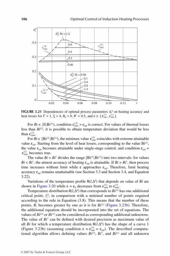
106 Optimal Control of Induction Heating Processes
For Bi ∈ [0,Bi(3)), condition > εinf is correct. For values of thermal lossesless than Bi(3), it is possible to obtain temperature deviation that would be lessthan .
For Bi ∈ [Bi(3),Bi(1)), the minimax value coincides with extreme attainablevalue εinf. Starting from the level of heat losses, corresponding to the value Bi(1),the value εinf becomes attainable under single-stage control, and condition εinf =
becomes true.The value Bi = Bi* divides the range [Bi(3),Bi(1)) into two intervals: for values
Bi < Bi*, the utmost accuracy of heating εinf is attainable. If Bi > Bi*, then processtime increases without limit while ε approaches εinf. Therefore, limit heatingaccuracy εinf remains unattainable (see Section 3.3 and Section 3.4, and Equation3.22).
Variations of the temperature profile θ(l,∆0) that depends on value of Bi areshown in Figure 3.20 while ε = ε0 decreases from to .
Temperature distribution θ(l,∆0) that corresponds to Bi(3) has one additionalcritical point, lj
0, in comparison with a minimal number of points requiredaccording to the rule in Equation (3.8). This means that the number of thesepoints, R, becomes greater by one as it is for Bi(1) (Figure 3.23b). Therefore,the additional equation should be incorporated into the set of equations. Thevalues of Bi(3) or Bi(1) can be considered as corresponding additional unknowns.The value of Bi* can be defined with desired precision as maximum value ofall Bi for which a temperature distribution θ(l,∆0) has the shape of a curve 1(Figure 3.23b) (assuming condition ε = = εinf). The described computa-tional algorithm allows defining values Bi(3), Bi*, and Bi(1) and all unknown
FIGURE 3.21 Dependencies of optimal process parameters ∆i0 on heating accuracy and
heat losses for Γ = 1, ξ = 4, θ0 = 0, θ* = 0.5, and ε ∈ [ , ].
0 0.02 0.04 0.06 0.08 0.10 0.12 ε
0.1
0.2
0.3
0.4
0.06
0.1
0.4
0.8
0.1 0.4 0.8 1.2
Δi0
Δ10; Bi = 1.2
Δ20; Bi = 0.06
(2) εmin
(2) εmin
(1) εmin
εmin( )2 εmin
( )1
εmin( )3
εmin( )3
εmin( )3
εmin( )1
εmin( )2 εmin
( )3
εmin( )3
DK6039_C003.fm Page 106 Monday, June 12, 2006 10:22 AM
© 2007 by Taylor & Francis Group, LLC
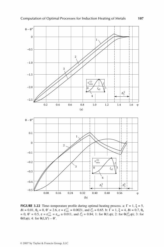
Computation of Optimal Processes for Induction Heating of Metals 107
FIGURE 3.22 Time–temperature profile during optimal heating process. a: Γ = 1, ξ = 5,Bi = 0.01, θ0 = 0, θ* = 2.6, ε = = 0.0021, and le2
0 = 0.65. b: Γ = 1, ξ = 4, Bi = 0.7, θ0
= 0, θ* = 0.5, ε = = εinf ≅ 0.011, and le20 = 0.84; 1: for θ(1,ϕ); 2: for 0θ(le2,ϕ); 3: for
θ(0,ϕ); 4: for θ(l,∆0) – θ*.
(b)
0 1
4
0.2 0.4 0.6 0.8
(a)
1.0 1.2 1.4 1.6 ϕ
ϕ
0
θ − θ∗
θ − θ∗
−0.5
−1.0
−1.5
−2.0
−2.5
1
2
3
4
0 1
0
0.1
−0.1
−0.2
−0.3
−0.4
−0.50.08 0.16 0.24 0.32 0.40 0.48 0.56
1
2
3
∆20
∆20 ∆3
0
le2
le2
l
l
εmin(2)
εmin(3)
εmin( )2
εmin( )3
DK6039_C003.fm Page 107 Monday, June 12, 2006 10:22 AM
© 2007 by Taylor & Francis Group, LLC
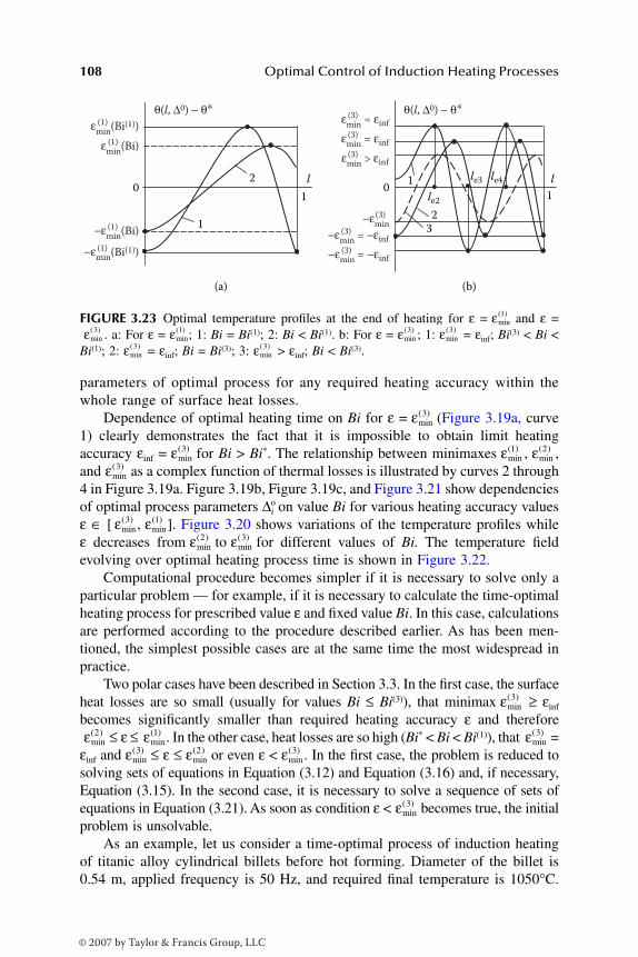
108 Optimal Control of Induction Heating Processes
parameters of optimal process for any required heating accuracy within thewhole range of surface heat losses.
Dependence of optimal heating time on Bi for ε = (Figure 3.19a, curve1) clearly demonstrates the fact that it is impossible to obtain limit heatingaccuracy εinf = for Bi > Bi*. The relationship between minimaxes , ,and as a complex function of thermal losses is illustrated by curves 2 through4 in Figure 3.19a. Figure 3.19b, Figure 3.19c, and Figure 3.21 show dependenciesof optimal process parameters ∆i
o on value Bi for various heating accuracy valuesε ∈ [ , ]. Figure 3.20 shows variations of the temperature profiles whileε decreases from to for different values of Bi. The temperature fieldevolving over optimal heating process time is shown in Figure 3.22.
Computational procedure becomes simpler if it is necessary to solve only aparticular problem — for example, if it is necessary to calculate the time-optimalheating process for prescribed value ε and fixed value Bi. In this case, calculationsare performed according to the procedure described earlier. As has been men-tioned, the simplest possible cases are at the same time the most widespread inpractice.
Two polar cases have been described in Section 3.3. In the first case, the surfaceheat losses are so small (usually for values Bi ≤ Bi(3)), that minimax ≥ εinf
becomes significantly smaller than required heating accuracy ε and therefore≤ ε ≤ . In the other case, heat losses are so high (Bi* < Bi < Bi(1)), that =
εinf and ≤ ε ≤ or even ε < . In the first case, the problem is reduced tosolving sets of equations in Equation (3.12) and Equation (3.16) and, if necessary,Equation (3.15). In the second case, it is necessary to solve a sequence of sets ofequations in Equation (3.21). As soon as condition ε < becomes true, the initialproblem is unsolvable.
As an example, let us consider a time-optimal process of induction heatingof titanic alloy cylindrical billets before hot forming. Diameter of the billet is0.54 m, applied frequency is 50 Hz, and required final temperature is 1050°C.
FIGURE 3.23 Optimal temperature profiles at the end of heating for ε = and ε =. a: For ε = ; 1: Bi = Bi(1); 2: Bi < Bi(1). b: For ε = ; 1: = εinf; Bi(3) < Bi <
Bi(1); 2: = εinf; Bi = Bi(3); 3: > εinf; Bi < Bi(3).
0
(b)
1
1
23
1
l l
(a)
1
20
le2
le3 le4
θ(l, ∆0) − θ∗ θ(l, ∆0) − θ∗ ε
min(Bi(1))(1)
εmin
(Bi)(1)
εmin
= εinf(3)
εmin
= εinf(3)
εmin
> εinf(3)
−εmin(3)
−εmin
= −εinf(3)
−εmin
= −εinf(3) −ε
min(Bi(1))(1)
−εmin
(Bi)(1)
εmin( )1
εmin( )3 εmin
( )1 εmin( )3 εmin
( )3
εmin( )3 εmin
( )3
εmin( )3
εmin( )3 εmin
( )1 εmin( )2
εmin( )3
εmin( )3 εmin
( )1
εmin( )2 εmin
( )3
εmin( )3
εmin( )2 εmin
( )1 εmin( )3
εmin( )3 εmin
( )2 εmin( )3
εmin( )3
DK6039_C003.fm Page 108 Monday, June 12, 2006 10:22 AM
© 2007 by Taylor & Francis Group, LLC

Computation of Optimal Processes for Induction Heating of Metals 109
Let us assume that the maximal surface density of heating power is about 106kW/m2. The average values of electromagnetic and thermophysical parametersare:
, , ,
whereρ is electrical resistivity.λ is thermal conductivity of the metal.a is temperature conductivity of heated material.
Let us assume that the average value of convection heat transfer coefficientduring the heating is equal to 35 to 40 W/(m2 ⋅ °C), which corresponds to thevalue of Bi ≅ 0.7 for surface thermal losses. The heating process is describedprecisely enough by model (Equation 1.27 through Equation 1.35). Using thesystem of relative units discussed in Chapter 1, we can obtain θ* = 0.5 and ξ =4 for the case when initial temperature equals ambient temperature of 30°C.
For considered initial data and calculated values of θ* and ξ, the soughtparameters of a time-optimal heating process can be obtained using computationresults presented in Figure 3.19 through Figure 3.21. Computational procedurehas been performed according to the algorithm described previously. For valuesξ = 4, θ* = 0.5, and Bi = 0.7 (Figure 3.19), the following results can be obtained:
= 0.075; = 0.0246; = εinf ≅ 0.01; Bi(3) = 0.031;
Bi* ≅ 0.460; Bi(1) = 1.400.
Therefore, Bi* < Bi = 0.7 < Bi(1).Results can be rewritten in absolute units as:
= 153°C; = 50.3°C; = εinf ≅ 21°C.
Corresponding values of optimal process intervals of heating and temperaturesoaking are presented in Table 3.1 for minimax errors. The minimax = 153°Cdefines nonuniformity of heating, which is typically unacceptable for the majorityof hot forming applications where the higher accuracy is usually required — i.e.,ε < .
If = 50.3°C ≤ ε < 153°C, then it is necessary to provide two-stage optimalcontrol, i.e., “heating–temperature soaking” mode. However, in the case of εinf =
= 21°C ≤ ε < = 50.3°C, it would be necessary to apply a three-stagecontrol process that would include heating, soaking, and reheating process stages.
Utmost heating accuracy coincides with minimax and it appears unat-tainable under conditions Bi = 0.7 > Bi* = 0.46. Therefore, for ε ≤ 21°C, the
ρ = ⋅ ⋅−180 10 8 Ohm m λ =⋅
14 0
W
m Ca
m
s= ⋅ −4 34 10 6
2
.
εmin( )1 εmin
( )2 εmin( )3
εmin( )1 εmin
( )2 εmin( )3
εmin( )1
εmin( )1
εmin( )2
εmin( )3 εmin
( )2
εmin( )3
DK6039_C003.fm Page 109 Monday, June 12, 2006 10:22 AM
© 2007 by Taylor & Francis Group, LLC
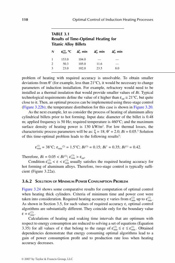
110 Optimal Control of Induction Heating Processes
problem of heating with required accuracy is unsolvable. To obtain smallerdeviations from θ* (for example, less than 21°C), it would be necessary to changeparameters of induction installation. For example, refractory would need to beinstalled as a thermal insulation that would provide smaller values of Bi. Typicaltechnological requirements define the value of ε higher than εinf ≅ 21°C, but quiteclose to it. Then, an optimal process can be implemented using three-stage control(Figure 3.22b); the temperature distribution for this case is shown in Figure 3.20.
As the next example, let us consider the process of heating of aluminum alloycylindrical billets prior to hot forming. Input data: diameter of the billet is 0.48m; applied frequency is 50 Hz; required temperature is 460°C; and the maximumsurface density of heating power is 130 kW/m2. For low thermal losses, thecharacteristic process parameters will be as: ξ = 18; θ* = 2.0; Bi = 0.05.5 Solutionof this time-optimal problem leads to the following results5:
= 38°C; εmin(2) = 1.5°C; Bi(3) = 0.15; Bi* = 0.35; Bi(1) = 0.42.
Therefore, Bi = 0.05 < Bi(3); > εinf.Condition < ε < usually satisfies the required heating accuracy for
hot forming of aluminum alloys. Therefore, two-stage control is typically suffi-cient (Figure 3.22a).
3.6.2 SOLUTION OF MINIMUM POWER CONSUMPTION PROBLEM
Figure 3.24 shows some comparative results for computation of optimal controlwhen heating thick cylinders. Criteria of minimum time and power cost weretaken into consideration. Required heating accuracy ε varies from up to .As shown in Section 3.5, for such values of required accuracy ε, optimal controlalgorithms are substantially different. They coincide only for the boundary valueε = .
Calculations of heating and soaking time intervals that are optimum withrespect to energy consumption are reduced to solving a set of equations (Equation3.35) for all values of ε that belong to the range of ≤ ε ≤ . Obtaineddependencies demonstrate that energy consuming optimal algorithms lead to again of power consumption profit and to production rate loss when heatingaccuracy decreases.
TABLE 3.1Results of Time-Optimal Heating for Titanic Alloy Billets
N (N)εεεεmin, °°°°C ∆∆∆∆1,0 min ∆∆∆∆2,
0 min ∆∆∆∆3,0 min
1 153.0 104.0 — —2 50.3 105.0 11.6 —3 23.0 102.0 23.5 8.0
εmin( )1
εmin( )3
εmin( )2 εmin
( )3
εmin( )2 εmin
( )1
εmin( )2
εmin( )2 εmin
( )1
DK6039_C003.fm Page 110 Monday, June 12, 2006 10:22 AM
© 2007 by Taylor & Francis Group, LLC
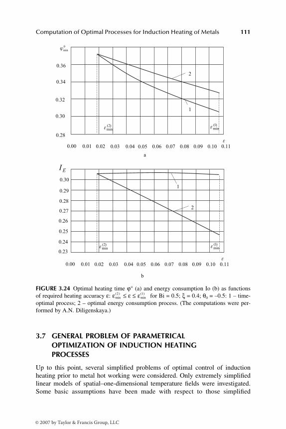
Computation of Optimal Processes for Induction Heating of Metals 111
3.7 GENERAL PROBLEM OF PARAMETRICAL OPTIMIZATION OF INDUCTION HEATING PROCESSES
Up to this point, several simplified problems of optimal control of inductionheating prior to metal hot working were considered. Only extremely simplifiedlinear models of spatial–one-dimensional temperature fields were investigated.Some basic assumptions have been made with respect to those simplified
FIGURE 3.24 Optimal heating time ϕ° (a) and energy consumption Io (b) as functionsof required heating accuracy ε: ≤ ε ≤ for Bi = 0.5; ξ = 0.4; θ0 = –0.5: 1 – time-optimal process; 2 – optimal energy consumption process. (The computations were per-formed by A.N. Diligenskaya.)
a
2
1
)2(min
)1(min
0.36
0.34
0.32
0.30
0.28
0min
0.00 0.01 0.02 0.03 0.04 0.05 0.06 0.07 0.08 0.09 0.10 0.11
2
1
)2(min
)1(min
0.30
EI
b0.00 0.01 0.02 0.03 0.04 0.05 0.06 0.07 0.08 0.09 0.10 0.11
0.29
0.28
0.27
0.26
0.25
0.24
0.23
b
εmin( )2 εmin
( )1
DK6039_C003.fm Page 111 Monday, June 12, 2006 10:22 AM
© 2007 by Taylor & Francis Group, LLC
112 Optimal Control of Induction Heating Processes
problems. This includes, but is not limited to, using one-dimensional mathemat-ical models and neglecting nonlinearity of physical properties of the heatedmetals. Obviously, these assumptions could result in noticeable error for certainapplications. More precise models should take into consideration the severalcomplex and interrelated phenomena, including nonlinear properties (particularlywhen heating ferromagnetic billets above the Curie temperature) as well as two-or three-dimensional distribution of electromagnetic and thermal fields. In addi-tion, it might be necessary to consider several additional criteria or even theircombination. The whole set of additional technological constraints, disturbances,and uncertainties of a controlled system can be added as well (see Chapter 2).
It will be shown next that even taking into consideration practically all of themost important factors, it is often possible to perform preliminary parameteriza-tion of sought optimal control inputs. Parameterization of the control problemrequires specifying control input function by one or more variables. In cases likethese, the initial problem is reduced to searching for number N and optimal valuesof parameters ∆i, 1, 2, …, N that uniquely specify optimal control input (similarlyto Equation 2.27 and Figure 2.8). These parameters make different physical sensein different problems.
The chosen cost function, I(∆), and temperature distribution, t(x,∆), withinbillet volume Ω at the end of the heating process are functions of the set ∆ = (∆1,∆2, …, ∆N) and vector x of spatial coordinates. Vector x includes coordinatesalong which the temperature distribution is essentially nonuniform. Let us assumenow that these functions could be obtained in an explicit form using any knownmethod.
Let us also assume that, at the end of a heating process, it is necessary toprovide absolute temperature deviation ε of final temperature t(x,∆) from thepreassigned one, t*, similarly to Equation (2.30). As was shown in Chapter 2,similarly to Equation (2.34) for the simplest time-optimal problem, the task ofvector ∆0 = (∆1,
0 ∆2,0 …, 0∆N) search can be reduced to the following problem of
mathematical programming:
(3.38)
The problem in Equation (3.38) proves to be more difficult than those inEquation (2.34) or Equation (2.42). This is due to the fact that the cost functionis more complicated in comparison with the simpler ones that correspond toEquation (2.31) and Equation (2.41). In addition, the basic difficulties arise herebecause the spatial distribution of final temperature t(x,∆) could be noticeablydifferent compared to cases described earlier. These features primarily deal withnonlinear and multidimensional models of temperature fields.
Nevertheless, it is possible to show5 that, if some preliminary conditions aremet, then the optimal control method offered in the present text could be applied
I
t x tx
∆
Φ ∆ ∆
∆
Ω
( ) →
( ) = ( ) − ≤
∈
min;
max , .* ε
DK6039_C003.fm Page 112 Monday, June 12, 2006 10:22 AM
© 2007 by Taylor & Francis Group, LLC
Computation of Optimal Processes for Induction Heating of Metals 113
in its basic aspects to the general case (Equation 3.38). Of course, not all optimalcontrol results discussed earlier for the simplified IHP models can be easilytransferred for these more complex cases.
High generality of the basic property of the temperature distribution at theoptimal process end allows one to extend the area of application of the consideredmethod onto the wide problem variety. Similarly to Equation (3.7) and Equation(3.8), the number, R, of points within billet where maximum admissible deviationsare reached, is not less than number N of parameters of sought optimal control.This rule does not depend on types of IHP models, cost functions, technologicalconstraints, control inputs, and other factors.5
The analysis similar to the one provided in Section 3.1 for time-optimal IHPallows writing alternance property in the form similar to relations in Equation(3.7) and Equation (3.8):
(3.39, 3.40)
where are coordinates of points within the billet, where maxi-mum deviations of the final temperature from the prescribed one are reached.
These deviations are equal to ε. In contrast to Equation (3.7), in cases ofmultidimensional thermal models, we consider xj
0 as a set of jth point coordinatesalong a corresponding axis. As stated before, in Equation (3.40) representsthe maximal possible value of the utmost heating accuracy — i.e., minimalpossible deviation from t*. Such accuracy can be achieved by applying controlactions explicitly characterized by a set of N parameters vector ∆ = (∆1, ∆2, …, ∆N).
In the general case (Equation 3.38) and similarly to time-optimal controlinputs, it is assumed that control inputs could be defined by this set of N para-meters, ∆I, for which the sequence of inequalities of the type in Equation (3.1)holds true:
. (3.41)
Let us notice that, in the general case (Equation 3.38), the condition inEquation (3.3) is no longer true. This condition directly links the number, N, withthe place of preset value, ε, in the series of inequalities in Equation (3.41). Thisfact was discussed earlier, considering as an example an optimization of consumedenergy of induction heater (Section 3.5).
Generally speaking, Equation (3.40) is only true under assumption that anumber, N, is known and does not necessarily correspond to a condition (Equation3.3).2 This situation differs from the case described earlier by Equation (3.8),where the number of optimal control parameters N directly depends on ε.
t x t j R
RN if
j
N
( , ) , , , ..., ;
, ;
*
min( )
0 0 1 2∆ − = =
=>
ε
ε ε
NN if N+ =
1, ,min
( )ε ε
x j Rj0 1∈ =Ω, ,
εmin( )N
ε ε ε ε εmin( )
min( )
min( )
min( )... ...1 2 1> > > > > >+N N
mmin( )
inf
*N = >ε 0
DK6039_C003.fm Page 113 Monday, June 12, 2006 10:22 AM
© 2007 by Taylor & Francis Group, LLC
114 Optimal Control of Induction Heating Processes
Properties in Equation (3.39) and Equation (3.40) mean that, for knownnumber N that corresponds to required accuracy ε, such R (number of the pointsxi
0 within billet) will be necessarily found, which is related with N by Equation(3.40). Thus, in reality the actual number of these points can be greater than R,and the problem of defining the value N should be solved separately for eachspecific case.
Properties in Equation (3.39) and Equation (3.40) are correct, taking intoconsideration preliminary conditions that prove to be formal enough and notrestrictive. As a rule, they are met in practice for problems of actual IHP optimi-zation.2,5 The only exception deals with simplified and uncommon cases from apractical standpoint when requirements to heating accuracy are insignificant and“automatically” satisfied for the optimal control solution ∆ = ∆0. This case takesplace if ∆0 is a minimum point of I(∆), and therefore
(3.42)
Vector ∆0 could be found from these N equations. Solution of the problem inEquation (3.38) can be found relatively easily by considering the set of N equa-tions that should be solved with respect to unknowns ∆0 for given I(∆).
We shall assume further that, considering only the main variant with an“active” constraint role in Equation (3.38), ∆0 is not an extremum point of I(∆).Similarly to techniques described earlier in this chapter, relations in Equation(3.39) and Equation (3.40) create potential possibilities for their transformationinto corresponding systems of equations with respect to sought parameters of theoptimal process. In comparison with simple IHP optimization, several importantpeculiarities take place in this case.
One of them deals with the nature of final spatial temperature distribution.Its accurate computation represents a much more difficult problem than a simpledefinition of curve θ(l,∆0) obtained from considering a one-dimensional mathe-matical model in a time-optimal control problem. Actually, in cases like this,when general alternance equalities (Equation 3.9) are not met, variants of loca-tions of points xj
0 could not be unambiguously set a priori. Therefore, finaltemperature distribution and set of governing equations also could not be foundeasily. In addition, the definition of function t(x,∆) in the explicit form representsthe separate task for complex IHP models.
Nevertheless, the alternance method can be successfully applied for a widevariety of specific IHP optimization problems of the type in Equation (3.38).2,5,7–21
This conclusion is based on the following general reasons. In the great majorityof cases, N = 1 for ε = in Equation (3.38). This simplest case corresponds tothe most typical modes of induction heating applied to various models and costfunctions. It is relatively easy in this case to predict the time history and the shapeof final temperature profile along the radius/thickness of the heated workpiece.If expression t(x,∆) ≡ t(x,∆1) is known, then conversion of relations in Equation
∂∂
= =Ii N
i
( ), , .
∆∆
0
0 1
εmin( )1
DK6039_C003.fm Page 114 Monday, June 12, 2006 10:22 AM
© 2007 by Taylor & Francis Group, LLC

Computation of Optimal Processes for Induction Heating of Metals 115
(3.39) and Equation (3.40) into the corresponding set of equations becomesstraightforward (as well as in Section 3.3).
It would be possible to determine ∆1 and using known numerical meth-ods. Under typical conditions for a given heating accuracy ε < , the soughtoptimal control (i.e., unknown vector ∆0) could be found by solving the problemin Equation (3.38) for the series of fixed values ε = ε′ descending by sufficientlysmall step dε starting from initial value . It can be done similarly to theprocedure suggested in Section 3.4 and applied to a particular example discussedin Section 3.6.
The continuous nature of the final temperature distribution and all optimalprocess parameters as functions of ε allows one to establish (using basic propertiesin Equation 3.39 and Equation 3.40) optimal final temperature profile. It ispossible to write a set of equations and to choose its initial approximation usingresults of a previous step. In the course of this algorithm implementation, thenumber N usually can be determined by some simple calculation experiments.This number grows with decreasing values of ε′.5 This procedure often becomessimpler if known physical features are employed.
The following chapters will detail the way in which the alternance methodis extended onto a wide range of IHP and IHI optimization problems for staticand continuous heaters as well as onto more general control problems for pro-duction complexes that involve interrelated heating and hot forming processes.Computational algorithms suggested later noticeably extend the optimizationtechnique, allowing its usage directly for optimal operational modes and optimalIHI design for the variety of technological processes.
The supposed method has some noticeable advantages in comparison withcomplicated and time-consuming numerical techniques developed for solution ofmathematical programming problems similar to those in Equation (3.38).22–24 Thismethod is based upon evident qualitative features of the physical nature of optimalinduction heating processes. These features are used in the course of a compu-tational procedure and also as effective means to check received results. Inaddition, these features allow one to find (depending on required heating accu-racy) the number and location of the points of maximal and minimal temperaturesat the end of an optimal process. All the foregoing allow a dramatic decrease inthe required amount of calculations by reduction of the wide range of initialoptimization problems to special, easy-to-solve sets of equations.
At the same time, the alternance method offers a way to calculate the maximalheating accuracy — i.e., values of minimaxes in Equation (3.41),including maximum achievable accuracy εinf = , within a particular class of thecontrol inputs. This opportunity represents a particular interest with respect to IHPtechnology. The alternance method also allows one to establish the outline of spatialfinal temperature distribution at the end of an optimal process for any given heatingaccuracy. This information could be used for creating technological charts and pro-grams and also for synthesis of optimal control systems with temperature feedback.
εmin( )1
εmin( )1
εmin( )1
εmin( ) *, ,i i N= 1
εmin( *)N
DK6039_C003.fm Page 115 Monday, June 12, 2006 10:22 AM
© 2007 by Taylor & Francis Group, LLC
116 Optimal Control of Induction Heating Processes
REFERENCES
1. Collatz, L. and Krabs, W., Approximations Theorie. Tschebyscheffsche Approxi-mation mit Anwendungen, B.G. Feubner, Stuttgart, 1973.
2. Rapoport, E.Ya., Alternance Method for Solving Applied Optimization Problems,Nauka, Moscow, 2000.
3. Butkovskii, A.G., Optimal Control Theory for Systems with Distributed Parame-ters, Nauka, Moscow, 1965.
4. Butkovskij, A.G., Malyj, S.A., and Andreev, Yu.N., Optimal Control of MetalsHeating, Metallurgy, Moscow, 1972.
5. Rapoport, E.Ya., Optimization of Induction Heating of Metals, Metallurgy, Mos-cow, 1993.
6. Ortega, J.M. and Rheinboldt, W.C., Iterative Solution of Nonlinear Equations inSeveral Variables, Academic Press, New York and London, 1970.
7. Rapoport, E.Ya., Exact method in problems of optimization of nonstationary heatconductivity processes, Izvestia AN SSSR, Energetika i transport, 4, 137, 1978.
8. Rapoport, E.Ya., Moving control in optimization problems for induction heatingof metals, in Mobile Control of Distributed Systems, Nauka, Moscow, 82, 1979.
9. Rapoport, E.Ya., Particular optimization problems for modes of metal heatingprior to hot working, Physica i himija obrabotki materialov, 3, 54, 1984.
10. Rapoport, E.Ya. and Zimin, L.S., Optimal control of slabs induction heating priorto rolling, Physica i himija obrabotki materialov, 3, 21, 1986.
11. Rapoport, E.Ya., Method for computation of optimal processes of materials heattreatment, Physica i himija obrabotki materialov, 5, 5, 1987.
12. Pleshivtseva, Yu.E. et al., Spatial–time control of nonstationary heat transfer pro-cesses, Vestnik SamGTU, 1, 208, 1994.
13. Rapoport, E.Ya., Optimization of induction heating processes, Proc. 40th Int.Wissenschaftliches Kolloquium, Technische Universitaet Ilmenau, Thueringen, 4,48, 1995.
14. Rapoport, E.Ya., Parametric optimization of coupled electromagnetic and temper-ature fields in induction heating, Proc. Int. Symp. Electromagn. Fields Electr. Eng.(ISEF’95), Thessaloniki, 319, 1995.
15. Rapoport, E.Ya., Alternance properties of optimal temperature distribution andcomputational algorithms in problems of induction heating processes parametricoptimization, Proc. Int. Induction Heating Semin. (IHS-98), Padua, 443, 1998.
16. Rapoport, E.Ya., Pleshivtseva, Yu.E., and Livshits, M.Yu., Alternance method inproblems of induction heating processes: basic principles and experience of appli-cations, ISEF'99, Proc. Int. Symp. Electromagn. Fields Electr. Eng., Pavia, 141,1999.
17. Rapoport, E.Ya. and Pleshivtseva, Yu.E., Optimal control of electric heating bymobile internal sources, Proc. Int. Semin. Heating Internal Sources (HIS-01),Padua, 667, 2001.
18. Pleshivtseva, Yu.E. et al., Potentials of optimal control techniques in inductionthrough heating for forging, in Proc. Int. Sci. Colloquium Modeling for Electro-magn. Process., Hannover, 145, 2003.
19. Pleshivtseva, Yu.E. et al., Optimal control techniques in induction through heatingfor forging, in Proc. Int. Symp. Heating Electromagn. Sources HES-04, Padua,97, 2004.
DK6039_C003.fm Page 116 Monday, June 12, 2006 10:22 AM
© 2007 by Taylor & Francis Group, LLC
Computation of Optimal Processes for Induction Heating of Metals 117
20. Rapoport, E.Ya., Livshits, M.Yu, and Pleshivtseva, Yu.E., Alternance method inoptimization problems for processes of technological thermal physics: basics oftheory, computational algorithms, experience of application, TeplomassoobmenMMF-2000, Minsk, 3, 298, 2000.
21. Rapoport, E.Ya. and Pleshivtseva, Yu.E., Special optimization methods in heat-conductivity inverse problems, Izvestia RAN, Energetica, Moscow, 5, 144, 2002.
22. Demjanov, V.F. and Malozemov, V.N., Introduction in Minimax, Nauka, Moscow,1972.
23. Demjanov, V.F. and Vasiljev, L.V., Nondifferentiable Optimization, Nauka, Mos-cow, 1981.
24. Polak, E., Semi-infinite optimization in engineering design, Lecture Notes inEconomics and Mathematical Systems, Springer–Verlag, New York, 215, 1981.
DK6039_C003.fm Page 117 Monday, June 12, 2006 10:22 AM
© 2007 by Taylor & Francis Group, LLC
119
4
Optimal Control of Static Induction Heating Processes
This chapter discusses the wide range of optimal control problems for staticinduction heating
of metals prior to hot forming. The suggested parametric opti-mization method will be used as a basis for solving optimization problems, takinginto consideration real-life production requirements. The variety of cost functionsapplied to static induction heating processes will be considered in this chapter.An overview of the most typical process restraints will be provided for linear andnonlinear, one- and two-dimensional, and deterministic and bounded nondeter-ministic models of static induction heating.
4.1 TIME-OPTIMAL CONTROL FOR LINEAR ONE-DIMENSIONAL MODELS OF STATIC IHP WITH CONSIDERATION OF TECHNOLOGICAL RESTRAINTS
Detailed description of the time-optimal problem for static induction heating hasbeen provided in Chapter 2 and Chapter 3 with respect to restraint on controlinput (see form of Equation 2.7). That restraint is defined by power supplylimitations (Section 2.5.1).
Metal heating processes impose the two most general requirements withregard to the temperature distribution during the heating process. The first require-ment demands that the maximum value
θ
max
(
ϕ
) of the temperature within theheated workpiece should be below a certain admissible value
θ
adm
. If this valuewill be exceeded, then irreversible adverse changes in material structural prop-erties (i.e., grain boundary liquation, burning, etc.) and even metal melting couldtake place.
Secondly, the temperature differences within the whole volume of the heatedworkpiece should be restricted during heating in such a way that the maximumvalue,
σ
max
(
ϕ
), of tensile thermal stresses
σ
(
l
,
ϕ
) (due to thermal gradients) wouldnot exceed prescribed admissible value
σ
adm
, which corresponds to ultimate stresslimit of the heated material (see Section 2.5.2). Additional technological con-straints add complexity to the OCP solution and appropriate computational pro-cedures.
1
In the present section, we shall extend the alternance method to the
DK6039_C004.fm Page 119 Thursday, June 8, 2006 12:34 PM
© 2007 by Taylor & Francis Group, LLC
120
Optimal Control of Induction Heating Processes
solution of OCP with additional restraints applied to the linear one-dimensionalmodel of static heating process.
4.1.1 G
ENERAL
O
VERVIEW
OF
O
PTIMAL
H
EATING
P
OWER
C
ONTROL
An internally generated heating power is the most significant process parameterthat affects temperature distribution within the inductively heated workpiece.Proper heating process control involves appropriate choice of the internal heatsources (eddy current) power density represented by function
F
(
ξ
,
l
,
ϕ
) =
W
(
ξ
,
l
)
u
(
ϕ
) in the right side of Equation (1.27). However, such control functionsin many cases are too complex to be practically applied
.
Therefore, it is importantto develop a set of particular control inputs that could be relatively easily appliedin engineering practice. At first look, this may seem a relatively simple processthat calls for the total consumed heating power
u
(
ϕ
) as control input. In thisrespect, voltage applied to the induction coil can be considered as a requiredcontrol function (see Section 2.4).
The time-optimal control problem (formulated in general form in Section2.8) will be considered for static heating with prescribed accuracy. The mathe-matical model is described by Equation (1.27) through Equation (1.35). Time-dependent heating power
u
(
ϕ
) is chosen as lumped control input restrained byEquation (2.7). However, in contrast to Section 2.8, the technological constraintsin Equation (2.11) and Equation (2.13) now will be taken into account. Therefore,it is necessary to select such control function
u
(
ϕ
) =
u
*
(
ϕ
) that provides steeringworkpiece initial temperature distribution to desired temperature
θ
*
with pre-scribed accuracy
ε
(according to Equation 2.25) in minimal optimal process timeunder conditions in Equation (2.11) and Equation (2.13).
It has been proved earlier (see Section 2.8) that the time-optimal controlalgorithm consists of alternating stages of heating with maximum power
u
≡
U
max
(heat ON) and subsequent soaking/cooling under
u
≡
0 (heat OFF) cycles. Con-sequently, optimal control
u
*
(
ϕ
) takes the form of Equation (2.27) (Figure 2.9).Let us now consider a solution of the optimal problem subject to additionalrestraints
.
Such a solution will look different compared to a solution of OCPdiscussed earlier in Section 2.8.
If the computations reveal that conditions in Equation (2.11) and Equation(2.13) are not violated under control input in the form of Equation (2.27) duringthe whole heating process, then the obtained OCP solution should be consideredas optimal. Thus, a necessity in variation of optimal control mode arises onlywhen at least one of inequalities in Equation (2.11) and Equation (2.13) does nothold true under the control input function (Equation 2.27). In this case, optimaltime-varying heating power can be defined according to arrangement of curves
θ
max
(
ϕ
) and
σ
max
(
ϕ
). Study of the shapes of curves
θ
max
(
ϕ
) and
σ
max
(
ϕ
) couldindicate in which process stage — heating under
u
*
(
ϕ
) =
U
max
or soaking under
u
*
(
ϕ
) = 0 — the control input should be varied to satisfy the requirements inEquation (2.11) and Equation (2.13).
DK6039_C004.fm Page 120 Thursday, June 8, 2006 12:34 PM
© 2007 by Taylor & Francis Group, LLC
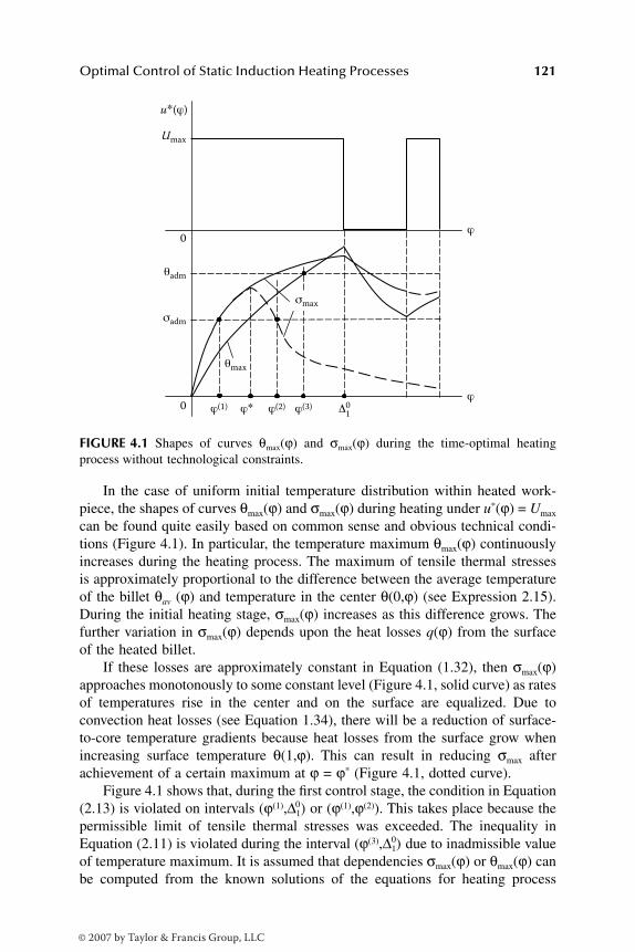
Optimal Control of Static Induction Heating Processes
121
In the case of uniform initial temperature distribution within heated work-piece, the shapes of curves
θ
max
(
ϕ
) and
σ
max
(
ϕ
) during heating under
u
*
(
ϕ
) =
U
max
can be found quite easily based on common sense and obvious technical condi-tions (Figure 4.1). In particular, the temperature maximum
θ
max
(
ϕ
) continuouslyincreases during the heating process. The maximum of tensile thermal stressesis approximately proportional to the difference between the average temperatureof the billet
θ
av
(
ϕ
) and temperature in the center
θ
(0,
ϕ
) (see Expression 2.15).During the initial heating stage,
σ
max
(
ϕ
) increases as this difference grows. Thefurther variation in
σ
max
(
ϕ
) depends upon the heat losses
q
(
ϕ
) from the surfaceof the heated billet.
If these losses are approximately constant in Equation (1.32), then
σ
max
(
ϕ
)approaches monotonously to some constant level (Figure 4.1, solid curve) as ratesof temperatures rise in the center and on the surface are equalized. Due toconvection heat losses (see Equation 1.34), there will be a reduction of surface-to-core temperature gradients because heat losses from the surface grow whenincreasing surface temperature
θ
(1,
ϕ
). This can result in reducing
σ
max
afterachievement of a certain maximum at
ϕ
=
ϕ
*
(Figure 4.1, dotted curve).Figure 4.1 shows that, during the first control stage, the condition in Equation
(2.13) is violated on intervals (
ϕ
(1)
,
∆
1
)
0
or (
ϕ
(1)
,
ϕ
(2)
). This takes place because thepermissible limit of tensile thermal stresses was exceeded. The inequality inEquation (2.11) is violated during the interval (
ϕ
(3)
,
∆
1
)
0
due to inadmissible valueof temperature maximum. It is assumed that dependencies
σ
max
(
ϕ
) or
θ
max
(
ϕ
) canbe computed from the known solutions of the equations for heating process
FIGURE 4.1
Shapes of curves
θ
max
(
ϕ
) and
σ
max
(
ϕ
) during the time-optimal heatingprocess without technological constraints.
0
u∗(ϕ)
ϕ(1)ϕ
ϕ
ϕ(2) ϕ(3) Δ10ϕ∗0
Umax
θadm
θmax
σmax
σadm
DK6039_C004.fm Page 121 Thursday, June 8, 2006 12:34 PM
© 2007 by Taylor & Francis Group, LLC
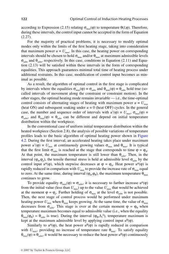
122
Optimal Control of Induction Heating Processes
according to Expression (2.15) relating
σ
max
(
ϕ
) to temperature
θ
(
l
,
ϕ
). Therefore,during these intervals, the control input cannot be accepted in the form of Equation(2.27).
For the majority of practical problems, it is necessary to modify optimalmodes only within the limits of the first heating stage, taking into considerationthat maximum power
u
≡
U
max
. In this case, the heating power on correspondingintervals should be chosen to hold
σ
max
and/or
θ
max
at maximum admissible levels
σ
adm
and
θ
adm
, respectively. In this case, conditions in Equation (2.11) and Equa-tion (2.13) will be satisfied within these intervals in the form of correspondingequalities. This approach guarantees minimal total time of heating process underadditional restraints. In this case, modification of control input becomes as min-imal as possible.
As a result, the algorithm of optimal control in the first stage is complicatedby intervals where the equalities σmax(ϕ) ≡ σadm and θmax(ϕ) ≡ θadm hold true (so-called intervals of movement along the constraint or constraint motion). In theother stages, the optimal heating mode remains invariable — i.e., the time-optimalcontrol consists of alternating stages of heating with maximum power u ≡ Umax
(heat ON) and subsequent soaking under u ≡ 0 (heat OFF) cycles. In the generalcase, the number and sequence order of intervals with u*(ϕ) ≡ Umax, σmax(ϕ) ≡σadm, and θmax(ϕ) ≡ θadm can be different and depend on initial temperaturedistribution within the workpiece.
In the conventional case of uniform initial temperature distribution within theheated workpiece (Section 2.8), the analysis of possible variations of temperatureprofiles leads to the basic algorithm of optimal heating power shown in Figure4.2. During the first interval, an accelerated heating takes place under maximumpower u*(ϕ) ≡ Umax at continuously growing values σmax and θmax. It is typicalthat the first limit σadm is reached at the stage that corresponds to time ϕ = ϕσ.At that point, the maximum temperature is still lower than θadm. Then, in theinterval (ϕσ,ϕp), the tensile thermal stress is held at admissible level σadm by thecontrol input uσ(ϕ), which stepwise decreases at ϕ = ϕσ. Heat power uσ(ϕ) israpidly reduced in comparison with Umax to provide the increase rate of σmax equalto zero. At the same time, during interval (ϕσ,ϕθ), the maximum temperature θmax
continues to grow.To provide equality σmax(ϕ) ≡ σadm, it is necessary to further increase uσ(ϕ)
from the initial value (less than Umax) up to the value Umax that would be achievedat the moment ϕ = ϕp. Further holding of σmax at the level σadm is not possible.Then, the next stage of control process would be performed under maximumheating power Umax when θmax keeps growing. At the same time, the value of σmax
decreases from σadm. This stage is over at the certain moment ϕ = ϕθ whentemperature maximum becomes equal to admissible value (i.e., when the equalityθmax(ϕθ) = θadm is true). During the interval (ϕθ,∆1
0), temperature maximum iskept at the maximum admissible level by applying control input uθ(ϕ).
Similarly to uσ(ϕ), the heat power uθ(ϕ) is rapidly reduced in comparisonwith Umax, providing no increase of temperature rate θmax. To satisfy equalityθmax(ϕ) ≡ θadm, it would be necessary to reduce the heat power uθ(ϕ) continuously
DK6039_C004.fm Page 122 Thursday, June 8, 2006 12:34 PM
© 2007 by Taylor & Francis Group, LLC

Optimal Control of Static Induction Heating Processes 123
(and therefore σmax(ϕ)). For ϕ > ∆1,0 the following stages are performed according
to the general control algorithm (Equation 2.27). The conditions θmax(ϕ) < θadm
and σmax(ϕ) < σadm usually are not violated over these stages because the valuesσmax and θmax decrease during even intervals under u(ϕ) ≡ 0. During odd intervals,these values do not reach their admissible levels.
As a result, the typical algorithm of the time-optimal heat power control withconsideration of the “real-life” technological constraints can be represented bythe following expression (Figure 4.2):
(4.1)
Certain optimal control functions (Equation 4.1) represent certain situationsor applications. If, during the stage when thermal stress is held at its maximum
FIGURE 4.2 Optimal control u*(ϕ), maximum temperature θmax, and thermal stress σmax
during the time-optimal process with technological constraints.
0
0
u∗(ϕ)
uσ uθ Δ20 Δ3
0
Δ10
Umax
θadm
θmax
σadm
σmax
ϕ
ϕ
ϕσ ϕp ϕθ
ϕ1 ϕ2 ϕ3
u
U
u
U
p
*
max
max
, , ;
, , ;
,ϕ
ϕ ϕ
ϕ ϕ ϕ ϕ
ϕ
σ
σσ
( ) =
∈( )
( ) ∈( )∈
0
ϕϕ ϕ
ϕ ϕ ϕ
θ
θθ
p
j
u
U
, ;
, , ;
max
( )( ) ∈( )
+ −( )
+
∆10
1
21 1 < < =
−, , , , ..., .ϕ ϕ ϕj j j N1 2 3
DK6039_C004.fm Page 123 Thursday, June 8, 2006 12:34 PM
© 2007 by Taylor & Francis Group, LLC

124 Optimal Control of Induction Heating Processes
permissible level σmax, the equality uσ(ϕ) = Umax is not reached until the timepoint ϕ = ϕθ, then the interval (ϕp,ϕθ) is excluded. In this case, instead of Equation(4.1), one can rewrite an optimal control function (Figure 4.3) as:
(4.2)
If, during the first heating stage under applying the maximum power, thetemperature maximum reaches admissible value θadm, but at the same time thevalue σmax still remains less than σadm, the interval of σmax holding should beexcluded (Figure 4.4):
FIGURE 4.3 Optimal control u*(ϕ) with a single stage of heating under maximum power,maximum temperature θmax, and thermal stress σmax during the time-optimal process withtechnological constraints.
0
0
u∗(ϕ)
uσ
uθ Δ20 Δ3
0
Δ10
Umax
θadm
θmax
σadm
σmax
ϕ
ϕϕσ ϕθ
ϕ1 ϕ2 ϕ3
u
U
u
u*
max , , ;
, , ;
,ϕ
ϕ ϕ
ϕ ϕ ϕ ϕ
ϕ ϕ
σ
σσ θ
θ( ) =
∈( )( ) ∈( )
( )
0
∈∈( )+ −( )
< < =+
−
ϕ
ϕ ϕ ϕ
θ , ;
, ,max
∆10
11
21 1 2
Uj
jj j ,, , ..., .3 N
DK6039_C004.fm Page 124 Thursday, June 8, 2006 12:34 PM
© 2007 by Taylor & Francis Group, LLC
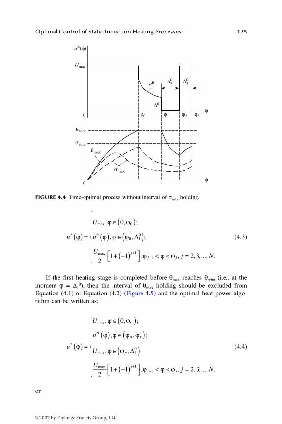
Optimal Control of Static Induction Heating Processes 125
(4.3)
If the first heating stage is completed before θmax reaches θadm (i.e., at themoment ϕ = ∆1
0), then the interval of θmax holding should be excluded fromEquation (4.1) or Equation (4.2) (Figure 4.5) and the optimal heat power algo-rithm can be written as:
(4.4)
or
FIGURE 4.4 Time-optimal process without interval of σmax holding.
0
0
u∗(ϕ)
uθ ∆20 ∆3
0
∆10
Umax
θadm
σmax
σadm
θmax
ϕ
ϕϕθ ϕ1 ϕ2 ϕ3
u
U
u
U
*
max
max
, , ;
, , ;ϕ
ϕ ϕ
ϕ ϕ ϕ
θ
θθ( ) =
∈( )
( ) ∈( )0
21
10∆
++ −( )
< < =
+
−1 2 31
1j
j j j N, , , , ..., .ϕ ϕ ϕ
u
U
u
U
p
*
max
max
, , ;
, , ;
,ϕ
ϕ ϕ
ϕ ϕ ϕ ϕ
ϕ
σ
σσ
( ) =
∈( )
( ) ∈( )∈
0
ϕϕ
ϕ ϕ ϕ
p
jj j
Uj
, ;
, , ,max
∆10
11
21 1 2
( )+ −( )
< < =+
− 33, ..., .N
DK6039_C004.fm Page 125 Thursday, June 8, 2006 12:34 PM
© 2007 by Taylor & Francis Group, LLC
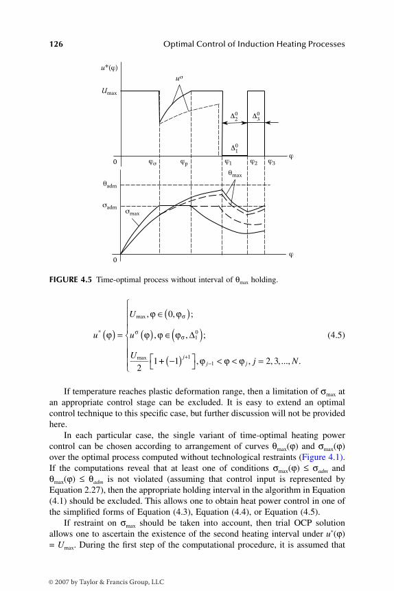
126 Optimal Control of Induction Heating Processes
(4.5)
If temperature reaches plastic deformation range, then a limitation of σmax atan appropriate control stage can be excluded. It is easy to extend an optimalcontrol technique to this specific case, but further discussion will not be providedhere.
In each particular case, the single variant of time-optimal heating powercontrol can be chosen according to arrangement of curves θmax(ϕ) and σmax(ϕ)over the optimal process computed without technological restraints (Figure 4.1).If the computations reveal that at least one of conditions σmax(ϕ) ≤ σadm andθmax(ϕ) ≤ θadm is not violated (assuming that control input is represented byEquation 2.27), then the appropriate holding interval in the algorithm in Equation(4.1) should be excluded. This allows one to obtain heat power control in one ofthe simplified forms of Equation (4.3), Equation (4.4), or Equation (4.5).
If restraint on σmax should be taken into account, then trial OCP solutionallows one to ascertain the existence of the second heating interval under u*(ϕ)= Umax. During the first step of the computational procedure, it is assumed that
FIGURE 4.5 Time-optimal process without interval of θmax holding.
0
0
u∗(ϕ)
uσ
Δ20 Δ3
0
Δ10
Umax
θadm
θmax
σadmσmax
ϕ
ϕϕσ ϕp ϕ1 ϕ2 ϕ3
u
U
u
U
*
max
max
, , ;
, , ;ϕ
ϕ ϕ
ϕ ϕ ϕ
σ
σσ( ) =
∈( )
( ) ∈( )0
21
10∆
++ −( )
< < =
+
−1 2 31
1j
j j j N, , , , ..., .ϕ ϕ ϕ
DK6039_C004.fm Page 126 Thursday, June 8, 2006 12:34 PM
© 2007 by Taylor & Francis Group, LLC
Optimal Control of Static Induction Heating Processes 127
uσ(ϕ) would not reach the value Umax. This means that, instead of Equation (4.1)or Equation (4.4), the control inputs in Equation (4.2) or Equation (4.5) shouldbe applied. If it turns out that the condition uσ(ϕθ) > Umax is true under the controlfunction in the form of Equation (4.2) or an expression uσ(∆1)
0 > Umax is valid inthe case of Equation (4.5), then the control inputs (Equation 4.1 or Equation 4.4)should be used. Time points ϕσ and ϕθ can be found as solutions of the followingequations:
σmax(ϕσ) = σadm; θmax(ϕθ) = θadm, (4.6)
where the functions σmax(ϕ) and θmax (ϕ) are known. Control functions uσ(ϕ) anduθ(ϕ) that provide holding in Equation (4.1) through Equation (4.5) can also bedetermined using the following conditions:
σmax(ϕ) σadm; θmax(ϕ) θadm. (4.7)
Let us assume that ϕσ, ϕθ, uσ(ϕ), and uθ (ϕ) in Equation (4.1) through Equation(4.5) are found; then, the shape of the optimal control algorithm is known. Atthe same time, the values of N control parameters remain unknown.Similarly to the solution described in Section 2.8, the values representdurations of control stages. However, in contrast to the time-optimal control inSection 2.8, in this case the heating mode in the first stage proves to be morecomplicated than heating under constant maximum power.
As a result, the considered time-optimal control problem is reduced to thespecial problem of mathematical programming in the form of Equation (2.34).To obtain the final temperature distribution θ(l,∆) in an explicit form, it is nec-essary to solve Equation (1.27) through Equation (1.35) with respect to powercontrol algorithms (Equation 4.1 through Equation 4.5). The values of ϕσ and ϕθand holding controls uσ(ϕ) and uθ(ϕ) can be found in the course of the compu-tational procedure.
4.1.2 POWER CONTROL DURING THE HOLDING STAGE
The holding stage in induction heating applications represents a special processwhen it is necessary to hold maximum temperature in any workpiece point at acertain permissible level. In other cases, in addition to temperature, the holdingstage incorporates holding thermal stresses.
Variation of temperature distribution during the heating cycle can be com-puted from Expression (1.36) after substitution of control functions in the formof Equation (4.1) through Equation (4.5) and using the relationship in Equation(2.15) between maximum stress σmax and temperature θ(l,ϕ). According to Equa-tion (1.38) and Equation (1.40) under θo(l) θav(ϕ) θo const, it is possibleto obtain the following results.1–5
1. The first equality in the set in Equation (4.6) can be rewritten withrespect to unknown time point ϕσ as the following equation:
∆i i N, ,= 1∆i i N, ,= 1
DK6039_C004.fm Page 127 Thursday, June 8, 2006 12:34 PM
© 2007 by Taylor & Francis Group, LLC

128 Optimal Control of Induction Heating Processes
, (4.8)
where
.
Equation (4.8) can be solved with required accuracy using well-knownnumerical methods.
2. The first equality in the set in Equation (4.7) is correct if thermal stressis held at the desired level utilizing control input uσ(ϕ), which evolvesin time according to exponential law as follows:
uσ(ϕ) ≅ a + be–β(ϕ–ϕσ), ϕ ∈ (ϕσ, ϕ*), (4.9)
where ϕ* = ϕp in Expression (4.1) or Expression (4.4), and ϕ* = ϕθ inEquation (4.2).The coefficients a, b, and β in Expression (4.9) can be calculated usingthe following relations:
, (4.10)
where
. (4.11)
These formulas take into account only the first and the second propernumbers µn
2 in Equation (2.29).3. The shape of temperature profile (Figure 3.4) is unchanged under
control input (Equation 4.1 through Equation 4.3) until the time ϕ =ϕθ. Therefore, the second equality in the set in Equation (4.6) tends tobe handled with the appropriate condition of obtaining maximum tem-perature in the workpiece’s internal point l = lmax at the time ϕ = ϕθ.Time ϕθ and coordinate le2(ϕθ) = lmax can be found by considering theequalities:
UA W
en n
nn
admn
maxγξ
µσ
σµ ϕσ( )
−( ) ==
∞−∑ 2
1
12
AK
Bi Bi Kn
n n n
n
σ µ µ µ
µ=
+( ) ( ) − + + −( )( )
2 1
1
1
2 2
Γ
Γ 22 µn( )
aL L
E Eb
E L E= +
+=
−( ) −1 2
22 1
2
1 22
2 12
22
12
1 2 2µ µµ µ
µ µ,
LL
E E E E
E E
E E
1
1 2 1 22
2 12
1 22
2 12
1
( )+( ) +( ) = +
+µ µβ µ µ
;22
L A W e E A W for n andn n n n n nn= ( ) −( ) = ( ) =−σ µ ϕ σξ ξσ1 12
; nn = 2
DK6039_C004.fm Page 128 Thursday, June 8, 2006 12:34 PM
© 2007 by Taylor & Francis Group, LLC

Optimal Control of Static Induction Heating Processes 129
. (4.12)
Here, temperature distribution θ(lmax,ϕθ) and temperature gradient∂θ(lmax,ϕθ)/∂l should be calculated according to the general expression(Equation 1.36) after substitution of heating power in the form ofEquation (4.1) through Equation (4.3) for time interval (0,ϕθ).The expressions for θ(lmax,ϕθ) and ∂θ(lmax,ϕθ)/∂l should be obtained inthe explicit form as functions of lmax and ϕθ. This allows transforminga set of equalities in Equation (4.12) into the set of two equations thatought to be solved with respect to unknowns lmax and ϕθ using knownnumerical methods.
4. Assuming that the time of holding the maximum temperature θmax inany workpiece point at the level θadm is relatively small, it is possibleto neglect a displacement of maximum temperature point during thisinterval and to obtain the control function uθ(ϕ). This control functioncan be obtained using a condition of holding temperature in point lmax
at its maximum permissible level. According to the second equationin the set in Equation (4.7) and similarly to Expression (4.9), theholding control function uθ(ϕ) can be obtained using the followingexponential form1–5:
uθ(ϕ) ≅ a + be–β(ϕ–ϕθ), ϕ ∈ (ϕθ, ∆01). (4.13)
The coefficients a, b, and β can be calculated using Equation (4.10).Here, instead of Equation (4.11), it is possible to assume:
,
(4.14)
where
.
5. If time required for heating is appreciably long, then the holdingtemperature at a point lmax under calculated control function uθ(ϕ) ofthe form in Equation (4.13) does not provide holding the maximum
θ ϕ θθ ϕ
θθl
l
ladmmax
max, ;,( ) = ∂ ( )
∂= 0
L AK
UE An n n n
n nn n= − ( )
=( ) ( )θ θθ µµ θ µ2 0 1
max
; WW n nn ξ( ) = =for and1 2
AK l
Bi Bi Kn
n n
n n
θ µ µµ µ
( ) = ( )+ + −( )( ) ( )
2
1
2
2 2 2
max ;Γ
θθ θ ϕ µθn nl l K l dl= ( ) ( )∫0
1
, Γ
DK6039_C004.fm Page 129 Thursday, June 8, 2006 12:34 PM
© 2007 by Taylor & Francis Group, LLC

130 Optimal Control of Induction Heating Processes
temperature in any workpiece point at the level θadm. As a rule, for suchheating modes, the following condition, θmax(ϕ) > θadm, is true for ϕ >ϕθ. In this case, the simple computational procedure is suggested todetermine optimal power control function uθ(ϕ), using its approxima-tion by piecewise constant function (Figure 4.6). The accuracy of theapproximation increases with the number, S, of discrete steps of dura-tion ϕ* and is held at acceptable level when S is big enough.
A sequence of optimization problems that could be reduced to solution ofthe system of equations (Equation 4.12) for fixed values ϕ(ν) = ϕθ + ˜νϕ*, ν =should be solved with respect to the control function u(v) and the point lmax.
(v) Foreach ν ∈ , a temperature distribution at the appropriate time point ϕ = ϕ(v)
can be calculated from Expression (1.36) under known control functions u(1), u(2),…, u(v–1) within the range (ϕθ,ϕ(v–1)). As a result, at time points ϕ(1), ϕ(2), …, ϕ(S),the obtained control functions u(ν), ν = allow one to hold the maximumtemperature at points , , …, at the level of θadm. This means that, foreach ϕ ∈ (ϕθ,∆1),
0 the condition θmax(ϕ) = θadm takes place and its accuracy dependsupon S. The values u(v) can be defined more precisely in the course of subsequentcomputation of optimal heating processes using the iteration method under apriori unknown value 0∆1.
To simplify implementation of optimal heating mode, it is possible to chooseconstant values of uc
σ and ucθ, which only approximately hold σmax and θmax at
the extreme admissible levels. In this case, the values ucσ and uc
θ should be definedusing the standard method — for example, by minimizing mean square deviationof σmax(ϕ) and/or θmax(ϕ) from σadm and θadm.
FIGURE 4.6 Approximation of holding control uθ(ϕ) by piecewise constant function.
u(1)
u(2)
u(ν)
uθ(ϕ)
∆10ϕθ ϕ(1) ϕ(2) ϕ(ν−1) ϕ(ν)
ϕ∗∼
ϕ
1, S
1, S
1, Slmax
( )1 lmax( )2 l S
max( )
DK6039_C004.fm Page 130 Thursday, June 8, 2006 12:34 PM
© 2007 by Taylor & Francis Group, LLC

Optimal Control of Static Induction Heating Processes 131
4.1.3 COMPUTATIONAL TECHNIQUE FOR OPTIMAL HEATING MODES, TAKING INTO CONSIDERATION TECHNOLOGICAL CONSTRAINTS
If the values ϕσ and ϕθ and functions uσ(ϕ) and uθ(ϕ) are known, then the finaltemperature distribution θ(l,∆) can be calculated from the basic formula in Equa-tion (1.36) by substituting control inputs in the form of Equation (4.1) throughEquation (4.5).
Functions uσ(ϕ) and uθ(ϕ) can be obtained in an exponential form as Equation(4.9) and Equation (4.13). Then, it is possible to write the following expressionthat describes θ(l,∆) under optimal control (Equation 4.1):
, (4.15)
where
(4.16)
Here, , aσ, bσ, βσ and aθ, bθ, βθ are constant coefficients for uσ (ϕ)
and uθ (ϕ) in Equation (4.9) and Equation (4.13), respectively.Therefore, we come to the problem in Equation (2.34); however, Expression
(4.15) and Expression (4.16) for computation of θ(l,∆) become more complicatedin comparison with Equation (2.28) and Equation (2.29). Expression for optimaltime-dependent heating power that is considered as a control function will alsobe more complex when technological constraints are taken into consideration.Therefore, previously discussed conclusions (Chapter 3) regarding an optimalspatial temperature distribution cannot be easily transferred to these cases.
Computational procedures described in Section 3.7 should be used to deter-mine the vector of optimal parameters ∆0 = (∆1,
0 ∆2,0 …, 0∆i). Our experience
shows1–5 that the established (in Chapter 3) shape of final temperature distribution
θ θξ µ
µl U
W K l
Bi Bi
n n
n
, max∆Γ
( ) = +( ) ( )
+ + −( )( )0 2 2
2
1 KKC
n
n
n2
1µ( )
⋅=
∞
∑
C e a e eb
enn
n
n n p n= − + −( ) + −µ ϕ
σµ ϕ µ ϕ σ
σ
µσ σ µµ β
2 2 2
12
2nn p p n
n n p
e
e e
2 2
2 2
ϕ β ϕ ϕ µ ϕ
µ ϕ µ ϕ
σ σ σ
θ
− −( ) −( ) +
+ − + aa e eb
en n nn
nθ
µ µ ϕ θ
θ
µ β ϕθ θµµ β
21
2 21 1
2
2∆ ∆ ∆−( ) + −
− − θθ θµ ϕ µ ϕ( ) −
+
=
−( ) +
+ −( ) − −∑
e en n
j
j
N
2 2 0
1 11
3
exp µµn m
m j
N
2 ∆=
∑
ϕ0
1
==∑∆i
i
N
DK6039_C004.fm Page 131 Thursday, June 8, 2006 12:34 PM
© 2007 by Taylor & Francis Group, LLC

132 Optimal Control of Induction Heating Processes
θ(l, ∆0) and its properties (including the condition in Equation 3.3) remainedunchanged when these properties were not in contradiction with constraints onσmax and θmax. The latter condition is always true in practice when the inequality(Equation 4.17) is valid for the required maximum admissible deviation ε:
ε ≤ θadm – θ*. (4.17)
According to the property in Equation (3.9), the maximum admissible devi-ations, θ(lj
0,∆0) – θ*, of the final temperature distribution from the required onearise with different signs for each pair of sequentially located points lj
0. Thismeans that these deviations are alternating at the points lj
0, where 0 ≤ l10 < l2
0 …< lR
0 ≤ 1 (Figure 3.11, Figure 3.13, etc.). Therefore, if the condition in Equation(4.17) is not met, then equality
θ(lk0,∆0) – θ* = ε (4.18)
violates the maximum temperature constraint (Equation 2.11) in a certain pointlk
0 ∈ [0,1].If, during the heating process, temperature drops within the heated workpiece
are substantially small, then the value of σmax proves to be less than maximumadmissible level σadm. This allows one to consider the inequality in Equation(4.17) as the single condition under which the restraints (Equation 2.11 andEquation 2.13) do not violate alternance properties of the final temperaturedistribution θ(l,∆0).
Let us consider the optimal heating process that satisfies the condition inEquation (4.17). The following computational procedure is suggested for deter-mining an optimal control algorithm for induction heating processes.
1. At the beginning, constraints should be neglected and the time-optimalcontrol problem should be solved assuming that there are no con-straints. This leads to definition of dependencies σmax(ϕ) and θmax(ϕ).As was mentioned in Section 4.1.1, the particular type of the optimalalgorithm of power control function during the first process stage canbe chosen from the set in Equation (4.1) through Equation (4.5),according to the shapes of curves θmax(ϕ) and σmax(ϕ).
2. In this case, the optimal control functions uσ(ϕ) and/or uθ(ϕ) and timesϕσ and ϕθ should be computed from expressions provided in Section4.1.2. In the general case of Equation (4.1), the values ϕσ, ϕθ, and lmax
represent roots of Equation (4.8) and the set in Equation (4.12). At thesame time, instant ϕp that satisfies inequality ϕσ < ϕp < ϕθ can bedetermined as a solution to the following equation:
aσ + bσe–βσ(ϕp–ϕσ) = Umax. (4.19)
DK6039_C004.fm Page 132 Thursday, June 8, 2006 12:34 PM
© 2007 by Taylor & Francis Group, LLC
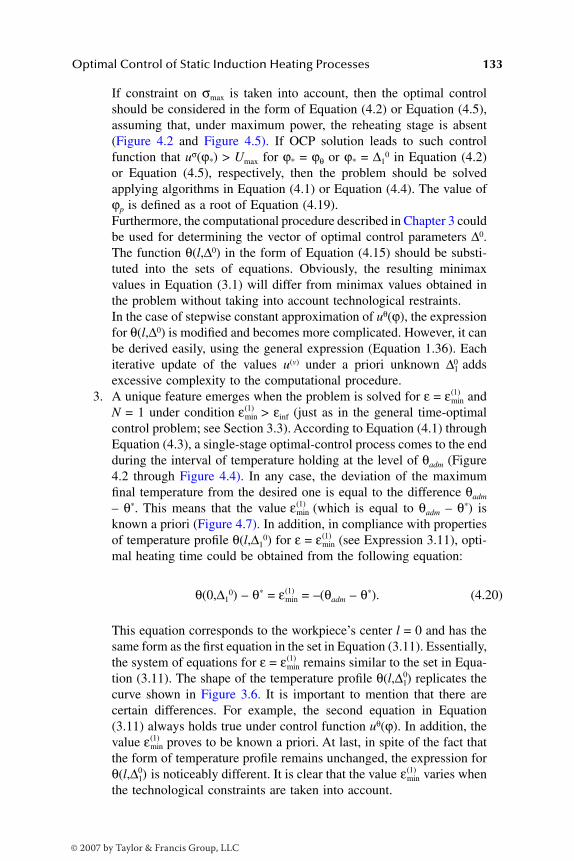
Optimal Control of Static Induction Heating Processes 133
If constraint on σmax is taken into account, then the optimal controlshould be considered in the form of Equation (4.2) or Equation (4.5),assuming that, under maximum power, the reheating stage is absent(Figure 4.2 and Figure 4.5). If OCP solution leads to such controlfunction that uσ(ϕ*) > Umax for ϕ* = ϕθ or ϕ* = ∆1
0 in Equation (4.2)or Equation (4.5), respectively, then the problem should be solvedapplying algorithms in Equation (4.1) or Equation (4.4). The value ofϕp is defined as a root of Equation (4.19).Furthermore, the computational procedure described in Chapter 3 couldbe used for determining the vector of optimal control parameters ∆0.The function θ(l,∆0) in the form of Equation (4.15) should be substi-tuted into the sets of equations. Obviously, the resulting minimaxvalues in Equation (3.1) will differ from minimax values obtained inthe problem without taking into account technological restraints.In the case of stepwise constant approximation of uθ(ϕ), the expressionfor θ(l,∆0) is modified and becomes more complicated. However, it canbe derived easily, using the general expression (Equation 1.36). Eachiterative update of the values u(v) under a priori unknown ∆1
0 addsexcessive complexity to the computational procedure.
3. A unique feature emerges when the problem is solved for ε = andN = 1 under condition > εinf (just as in the general time-optimalcontrol problem; see Section 3.3). According to Equation (4.1) throughEquation (4.3), a single-stage optimal-control process comes to the endduring the interval of temperature holding at the level of θadm (Figure4.2 through Figure 4.4). In any case, the deviation of the maximumfinal temperature from the desired one is equal to the difference θadm
– θ*. This means that the value (which is equal to θadm – θ*) isknown a priori (Figure 4.7). In addition, in compliance with propertiesof temperature profile θ(l,∆1
0) for ε = (see Expression 3.11), opti-mal heating time could be obtained from the following equation:
θ(0,∆10) – θ* = = –(θadm – θ*). (4.20)
This equation corresponds to the workpiece’s center l = 0 and has thesame form as the first equation in the set in Equation (3.11). Essentially,the system of equations for ε = remains similar to the set in Equa-tion (3.11). The shape of the temperature profile θ(l,∆1)
0 replicates thecurve shown in Figure 3.6. It is important to mention that there arecertain differences. For example, the second equation in Equation(3.11) always holds true under control function uθ(ϕ). In addition, thevalue proves to be known a priori. At last, in spite of the fact thatthe form of temperature profile remains unchanged, the expression forθ(l,∆1)
0 is noticeably different. It is clear that the value varies whenthe technological constraints are taken into account.
εmin( )1
εmin( )1
εmin( )1
εmin( )1
εmin( )1
εmin( )1
εmin( )1
εmin( )1
DK6039_C004.fm Page 133 Thursday, June 8, 2006 12:34 PM
© 2007 by Taylor & Francis Group, LLC
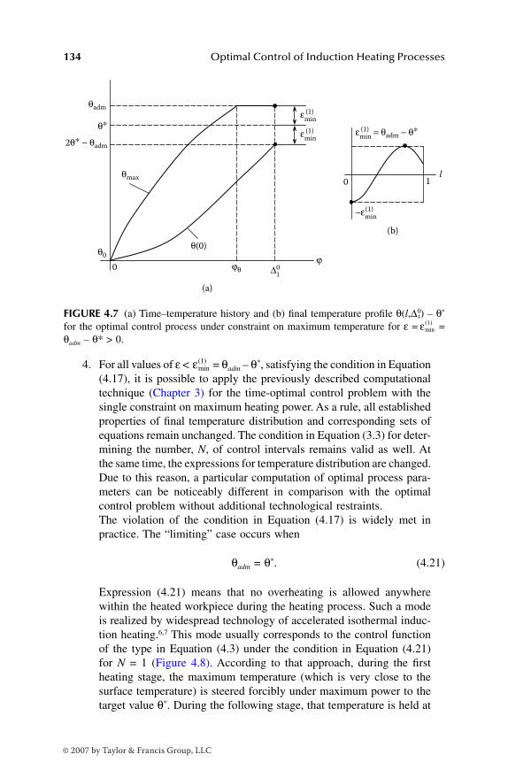
134 Optimal Control of Induction Heating Processes
4. For all values of ε < = θadm – θ*, satisfying the condition in Equation(4.17), it is possible to apply the previously described computationaltechnique (Chapter 3) for the time-optimal control problem with thesingle constraint on maximum heating power. As a rule, all establishedproperties of final temperature distribution and corresponding sets ofequations remain unchanged. The condition in Equation (3.3) for deter-mining the number, N, of control intervals remains valid as well. Atthe same time, the expressions for temperature distribution are changed.Due to this reason, a particular computation of optimal process para-meters can be noticeably different in comparison with the optimalcontrol problem without additional technological restraints.The violation of the condition in Equation (4.17) is widely met inpractice. The “limiting” case occurs when
θadm = θ*. (4.21)
Expression (4.21) means that no overheating is allowed anywherewithin the heated workpiece during the heating process. Such a modeis realized by widespread technology of accelerated isothermal induc-tion heating.6,7 This mode usually corresponds to the control functionof the type in Equation (4.3) under the condition in Equation (4.21)for N = 1 (Figure 4.8). According to that approach, during the firstheating stage, the maximum temperature (which is very close to thesurface temperature) is steered forcibly under maximum power to thetarget value θ*. During the following stage, that temperature is held at
FIGURE 4.7 (a) Time–temperature history and (b) final temperature profile θ(l,∆1)0 – θ*
for the optimal control process under constraint on maximum temperature for ε = =θadm – θ* > 0.
0 ∆10
θadm
θ0
ϕθ
θmax
θ(0)
ϕ
εmin(1)
εmin(1)
0 1l
εmin
= θadm − θ∗(1)
−εmin(1)
(a)
(b)
2θ∗ − θadm
θ∗
εmin( )1
εmin( )1
DK6039_C004.fm Page 134 Thursday, June 8, 2006 12:34 PM
© 2007 by Taylor & Francis Group, LLC

Optimal Control of Static Induction Heating Processes 135
this level until center temperature reaches the same value θ* withrequired accuracy.
It is not difficult to show that, even if the inverse sign of inequality (Equation4.17) takes place, i.e.,
ε > θadm – θ*, (4.22)
and, therefore, the correlations of the type in Equation (4.18) do not hold true,then even in this case all established properties of final temperature distributionθ(l,∆0) remain the same. This allows extending the proposed computational tech-nique to the special case in Equation (4.22).1 Keep in mind, though, that essentialfeatures arise in applying the alternance method.
One of these features deals with the necessity to replace equalities in Equation(4.18), which are not allowed due to the condition in Equation (4.22), by thefollowing equalities:
θ(lk,0 ∆0) – θ* = θadm – θ*, (4.23)
where lk0 are coordinates of points where the maximum admissible temperature
is reached.It is not necessary to incorporate these points into a set of equations because
conditions in Equation (4.23) are satisfied by control input uθ(ϕ). As a result, the
FIGURE 4.8 Optimal control u*(ϕ) and time–temperature history during accelerated iso-thermal induction heating.
0
0
u∗(ϕ)
uθ
Umax
∆10
∆10
ϕθ
ϕθ
ϕ
ϕ
θmax
θ(0)
εmin(1)θadm = θ∗
DK6039_C004.fm Page 135 Thursday, June 8, 2006 12:34 PM
© 2007 by Taylor & Francis Group, LLC
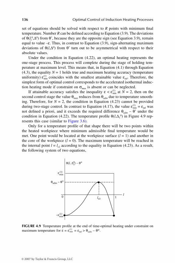
136 Optimal Control of Induction Heating Processes
set of equations should be solved with respect to R points with minimum finaltemperature. Number R can be defined according to Equation (3.9). The deviationsof θ(lj
0,∆0) from θ*, because they are the opposite sign (see Equation 3.9), remainequal to value –ε. Thus, in contrast to Equation (3.9), sign-alternating maximumdeviations of θ(l,∆0) from θ* turn out to be asymmetrical with respect to theirabsolute values.
Under the condition in Equation (4.22), an optimal heating represents theone-stage process. This process will complete during the stage of holding tem-perature at maximum level. This means that, in Equation (4.1) through Equation(4.3), the equality N = 1 holds true and maximum heating accuracy (temperatureuniformity) coincides with the smallest attainable value εinf. Therefore, thesimplest form of optimal control corresponds to the accelerated isothermal induc-tion heating mode if constraint on σmax is absent or can be neglected.
If attainable accuracy satisfies the inequality ε < at N = 2, then on thesecond control stage the value θmax reduces from θadm due to temperature smooth-ing. Therefore, for N = 2, the condition in Equation (4.23) cannot be providedduring two-stage control. In contrast to Equation (4.17), the value = εinf wasnot defined a priori, and it exceeds the required difference θadm – θ* under thecondition in Equation (4.22). The temperature profile θ(l,∆1
0) in Figure 4.9 rep-resents this case (similar to Figure 3.6).
Only for a temperature profile of that shape there will be two points withinthe heated workpiece where minimum admissible final temperature would bemet. One point would be located at the workpiece surface (l = 1) and another inthe core of the workpiece (l = 0). The maximum temperature will be reached inthe internal point l = le2 according to the equality in Equation (4.23). As a result,the following system of two equations,
FIGURE 4.9 Temperature profile at the end of time-optimal heating under constraint onmaximum temperature for ε = = εinf > θadm – θ*.
εmin( )1
εmin( )1
εmin( )1
0 le2
l1
θ(l, ∆10) − θ∗
εmin(1)
−εmin(1)
θadm − θ∗
εmin( )1
DK6039_C004.fm Page 136 Thursday, June 8, 2006 12:34 PM
© 2007 by Taylor & Francis Group, LLC

Optimal Control of Static Induction Heating Processes 137
(4.24)
should be solved with respect to two unknowns: optimal process time ∆10 and
value .Based on preliminary analysis, the following computational procedure can
be put into practice to solve the time-optimal control problem for the controlalgorithm of the type in Equation (4.1) through Equation (4.3) when at least oneconstraint on θmax is reached (Figure 4.10a and Figure 4.10b).
1. At the beginning, the optimal control problem should be solved forprescribed value ε = ε0 neglecting technological constraints. If thisproblem is solvable,* then this step should reveal that conditions inEquation (2.11) and Equation (2.13) are not violated over the computedheating cycle and, therefore, an optimal solution is obtained. Other-wise, the special type of optimal power control should be chosen fromthe set in Equation (4.1) through Equation (4.5). This selection willdepend upon the shapes of profiles θmax(ϕ) and σmax(ϕ) (Section 4.1).Furthermore, the next step should be taken.
2. Assuming that = θadm – θ* > εinf, the time-optimal control problemshould be solved under the additional technological constraints inEquation (2.11) and Equation (2.13) for providing temperature unifor-mity (heating accuracy) ε = (Figure 4.7). This problem can bereduced to solution of Equation (4.20).
3. The final surface temperature θ(l,∆1)0 can be calculated using the results
of the previous computation step and Expression (4.15) under l = 1, N= 1 (Figure 4.11). If the condition θ(1,∆1)
0 > θ(0,∆1)0 = –(θadm – θ*) is
true (curve 1, Figure 4.11), then the problem is solved as a result ofthe previous step, and step 5 should be performed next. Otherwise, itis necessary to perform step 4.
4. If results of the previous computation step satisfy the condition 0θ(1,∆1)< θ(0,∆1)
0 = –(θadm – θ*) (curve 2, Figure 4.11), then this means that theassumption regarding the value of is not valid (step 2), i.e., =εinf > θadm – θ*. Therefore, the case (Equation 4.22) takes place for ε= (Figure 4.9) and the set of equations in Equation (4.24) shouldbe solved with respect to ∆1
0 and .5. It is necessary to compare the prescribed numerical value of ε = ε0
with values of obtained in step 3 or step 4. If the prescribed valueof ε0 coincides with the obtained numerical value of minimax ,then the optimal control problem proves to be solved during one ofthe previous steps. If this value of ε satisfies the condition ε0 <
* Otherwise, the initial problem is not solvable.
θ θ ε
θ θ ε
1
0
10 1
10 1
, ;
, ;
*min
*min
∆
∆
( ) − = −
( ) − = −
( )
( )
εmin( )1
εmin( )1
εmin( )1
εmin( )1 εmin
( )1
εmin( )1
εmin( )1
εmin( )1
εmin( )1
εmin( )1
DK6039_C004.fm Page 137 Thursday, June 8, 2006 12:34 PM
© 2007 by Taylor & Francis Group, LLC
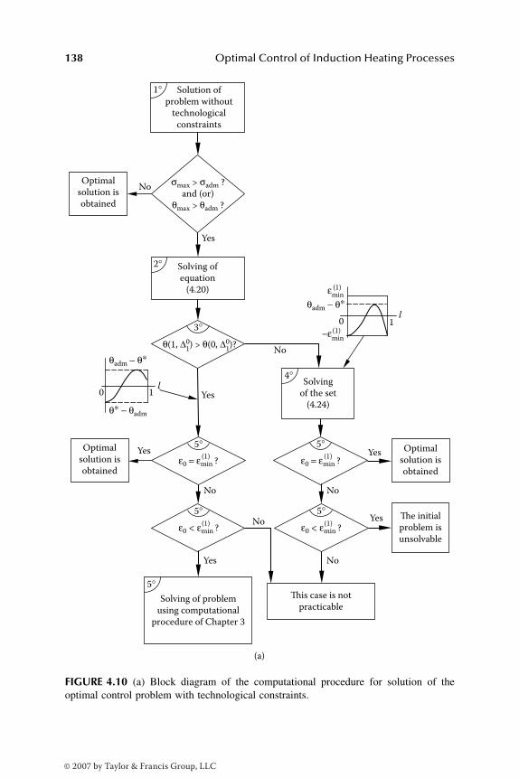
138 Optimal Control of Induction Heating Processes
FIGURE 4.10 (a) Block diagram of the computational procedure for solution of theoptimal control problem with technological constraints.
(a)
No
Yes
Yes
Solution of
problem without
technological
constraints
Solving of
equation
(4.20)
Solving of problem
using computational
procedure of Chapter 3
Solving
of the set
(4.24)
Optimal
solution is
obtained
Optimal
solution is
obtained
The initial
problem is
unsolvable
Optimal
solution is
obtained
Noσmax > σadm ?
and (or)
θmax > θadm ?
No
Yes
Yes
θ(1, ∆10) > θ(0, ∆
10)?
Yes
Yes
No
0 1l
0l
θadm − θ∗
θ∗ − θadm
(1)ε0 = εmin ?
(1)ε0 < εmin ?(1)ε0 < εmin ?
(1)ε0 = εmin ?
1
1°
This case is not
practicable
No
No
2°
3°
4°
5°
5°
5°
5°
5°
εmin(1)
−εmin(1)
θadm − θ∗
DK6039_C004.fm Page 138 Thursday, June 8, 2006 12:34 PM
© 2007 by Taylor & Francis Group, LLC
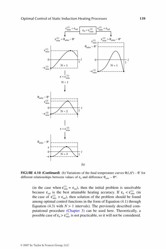
Optimal Control of Static Induction Heating Processes 139
(in the case when = εinf), then the initial problem is unsolvablebecause εinf is the best attainable heating accuracy. If ε0 < (inthe case of > εinf), then solution of the problem should be foundamong optimal control functions in the form of Equation (4.1) throughEquation (4.3) with N > 1 intervals). The previously described com-putational procedure (Chapter 3) can be used here. Theoretically, apossible case of ε0 > is not practicable, so it will not be considered.
FIGURE 4.10 (Continued) (b) Variations of the final temperature curves θ(l,∆0) – θ* fordifferent relationships between values of ε0 and difference θadm – θ*.
(b)
εmin
> εinf(1)
εmin(1)
ε < εmin(1)
εmin(1)
−εmin(1)
εmin
= εinf(1)
εmin
= θadm − θ∗(1) εmin
> θadm − θ∗(1)
θadm − θ∗
ε0 = εmin(1)
01
N = 1
N = 2
N = 3
N > 1
N = 1
l
1l
1l
1l
−εmin(1)
0
εmin(2)
ε
−ε
θadm − θ∗
θadm − θ∗
−εmin(2)
0
0
ε < εmin(2)
εmin( )1
εmin( )1
εmin( )1
εmin( )1
DK6039_C004.fm Page 139 Thursday, June 8, 2006 12:34 PM
© 2007 by Taylor & Francis Group, LLC

140 Optimal Control of Induction Heating Processes
Similarly to the optimal control problem with neglected technologicalrestraints (see Section 3.3 and Section 3.6), the optimal power control algorithmin Equation (4.1) through Equation (4.5) consists of N ≤ 3 stages that correspondto the most typical modes of induction heating. The computational procedure iskept identical to the one described in Section 3.4 and Section 3.6. It is importantto notice that the simplest possible cases are, at the same time, the most practicalcases. Variations of the temperature profile θ(l,∆0) for different relationshipsbetween values of ε0 and difference θadm – θ* that depends upon the value of ε0
are shown in Figure 4.10b. For the case of ε0 > θadm – θ*, the optimal controlprocess comes to the end after the single stage of isothermal soaking.
4.1.4 EXAMPLES
Figure 4.12 shows the results of the optimal processes of static heating underconstraints on σmax and θmax when the condition in Equation (4.17) is met.Computations have been performed according to the previously described tech-nique. Expressions for final temperature distribution θ(l,∆0) in the form of Equa-tion (4.15) and Equation (4.16) were used in all sets of equations. At least 20terms of infinite series in Equation (4.15) were included in governing equationsets. This example shows an optimal control mode when it is necessary to providethe maximum heating accuracy ε0 = using two-stage optimal control: heatingwith maximum power and subsequent soaking.
Figure 4.12a shows how power should be changed during the heating cycleaccording to the optimal control algorithm in Equation (4.1) for N = 2. It isobvious that the heating power uσ(ϕ) reaches maximum admissible value Umax
before reaching maximum temperature. Figure 4.12b shows the temperatureprofile θ(l,∆0) that takes place at the end of the optimal heating cycle. Onecan conclude that it is identical to the temperature profile for the similar case of
FIGURE 4.11 Variations of the final temperature profile for optimal process time obtainedfrom Equation (4.20). 1: under condition θ(l,∆1)
0 ≥ θ(0, 0∆1); 2: under condition 0θ(l,∆1)<θ(0,∆1
0).
0 1l
1
2
θadm − θ∗
−(θadm − θ∗)
θ(l, ∆10) − θ∗
εmin( )2
DK6039_C004.fm Page 140 Thursday, June 8, 2006 12:34 PM
© 2007 by Taylor & Francis Group, LLC
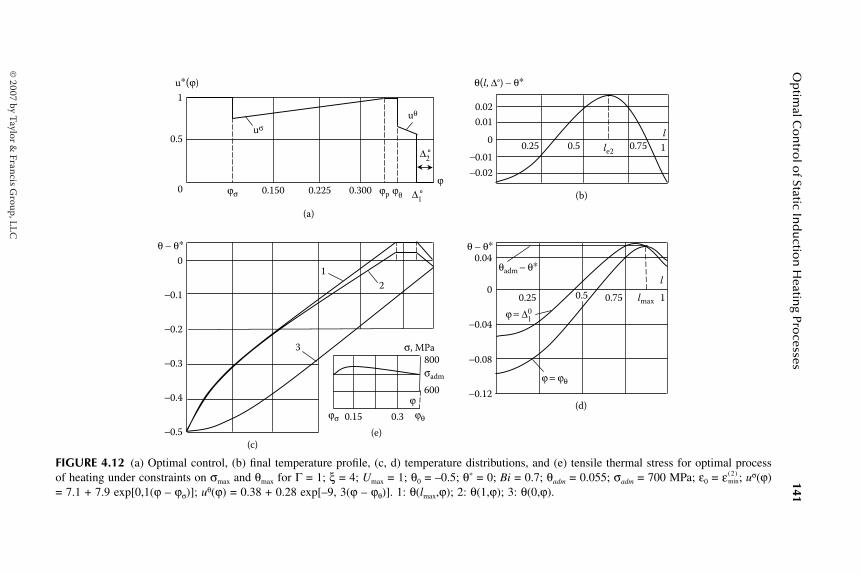
Op
timal C
on
trol o
f Static Ind
uctio
n H
eating Pro
cesses141
FIGURE 4.12 (a) Optimal control, (b) final temperature profile, (c, d) temperature distributions, and (e) tensile thermal stress for optimal processof heating under constraints on σmax and θmax for Γ = 1; ξ = 4; Umax = 1; θ0 = –0.5; θ* = 0; Bi = 0.7; θadm = 0.055; σadm = 700 MPa; ε0 = ; uσ(ϕ)= 7.1 + 7.9 exp[0,1(ϕ – ϕσ)]; uθ(ϕ) = 0.38 + 0.28 exp[–9, 3(ϕ – ϕθ)]. 1: θ(lmax,ϕ); 2: θ(1,ϕ); 3: θ(0,ϕ).
(a)
(b)
(d)
(c) (e)
0
−0.02
−0.01
0.02
0.01
0.25 0.5 0.75 1
uθ
∆2°
∆1°
uσ
1
0.5
0 0.150 0.225 0.300
u∗(ϕ)
ϕpϕσ
θ − θ∗ θ − θ∗
ϕθ
ϕ
0
−0.5
−0.4
−0.3
−0.2
−0.1
1
2
3
0.25 0.5 0.75 1
l 0
−0.04
−0.08
−0.12
0.04
σ, MPa
0.15 0.3
σadm
θadm − θ∗
ϕ = ∆10
ϕ = ϕθ
ϕϕσ ϕθ
600
800
le2
l
lmax
θ(l, ∆°) − θ∗
εmin( )2
DK
6039_C004.fm
Page 141 Thursday, June 8, 2006 12:34 PM
© 2007 by Taylor &
Francis Group, LLC
142 Optimal Control of Induction Heating Processes
ε0 = when the optimal control problem is solved neglecting technologicalconstraints (see Figure 3.8). It is clear that the inequality < θadm – θ* holdstrue under the condition in Equation (4.17).
Figure 4.12c shows time–temperature profiles for the two-stage heating cycle.Workpiece temperature reaches the maximum admissible value at some point lmax
at time ϕ = ϕθ. Maximum of temperature at the point lmax should be held at theadmissible level θadm during the time interval (ϕθ,∆1).
0 Control function uθ(ϕ) canbe written in the form of Expression (4.13). Temperature distributions at thebeginning (ϕ = ϕθ) and at the end (ϕ = ∆1)
0 of the holding stage are presented inFigure 4.12d. As seen in Figure 4.12e, optimal control uσ(ϕ) in the form ofEquation (4.9) provides holding σmax with reasonable accuracy during the interval(ϕσ,ϕp).
Let us now consider as an example an optimal heating process for the extremecase θadm = θ* meeting the condition in Equation (4.22) when the constraint onσmax is not taken into account (accelerated isothermal heating). The optimalprogram of heating power variation according to Expression (4.3) under N = 1is shown in Figure 4.13a. For ε0 = = εinf, the control function during the stageof isothermal soaking θ(lmax,ϕ) ≡ θadm takes the form of Equation (4.13). Depen-dence of this stage duration on required heating accuracy (ε0 > ) is presentedin Figure 4.13b. Figure 4.13c illustrates time–temperature history within work-piece volume for the case of ε0 = . Figure 4.13d shows the final temperaturedistribution for ε0 ≥ . Little fallibility could be seen in Figure 4.13d fortemperature maximum holding. This maximum shifts over time towards the billetcenter when temperature is held at the level of θadm = θ* at the single point lmax.
4.2 TIME-OPTIMAL PROBLEM, TAKING INTO CONSIDERATION THE BILLET TRANSPORTATION TO METAL FORMING OPERATION
4.2.1 PROBLEM STATEMENT
Let us consider the time-optimal control problem for the static induction heatingprocesses, taking into consideration billet transportation to the metal formingoperation. It is imperative to have a proper temperature state of the heated billetnot at the end of induction heating but at the beginning of the metal formingstage. After completion of the heating stage, it is necessary to transport the billetto the next technological operation (i.e., forging, rolling, stamping, upsetting,extrusion, etc.). Time of billet transportation depends upon the application, includ-ing but not limited to billet sizes, weight, layout of the machinery, and necessityof intermediate operation (for example, deposition of lubricant or scale removal).
Long transportation time leads to increase of the heat losses from the surfaceof the heated workpiece due to heat radiation and thermal convection. Therefore,transportation time should be minimized. However, due to previously mentionedtechnological restrictions, a transportation time is usually kept within 5 to 20 s.
εmin( )2
εmin( )2
εmin( )1
εmin( )1
εmin( )1
εmin( )1
DK6039_C004.fm Page 142 Thursday, June 8, 2006 12:34 PM
© 2007 by Taylor & Francis Group, LLC

Op
timal C
on
trol o
f Static Ind
uctio
n H
eating Pro
cesses143
FIGURE 4.13 Results of computation for the optimal process under constraint on θmax at θadm = θ* = 0 for Γ = 1; ξ = 4; Umax = 1; Bi = 0.7; θ0 =–0.5; uθ(ϕ) = 0.32 + 0.28 exp[–9.1(ϕ – ϕθ)]. a: Optimal control (ε0 = ); b: optimal process time (ε0 ≥ ); c: time–temperature history duringoptimal heating process (ε0 = ) d: final temperature distribution (ε0 ≥ ). 1: θ(lmax,ϕ); 2: θ(1,ϕ); 3: θ(0,ϕ); 4: θ(l,∆1
0) for ε0 = ; 5: θ(l,∆10)
for ε0 = 0.095 > ; 6: θ(l,ϕθ).
(a) (b)
(c) (d)
0
uθ
ϕθ
u∗
0.5
0.06 0.12 0.18 0.24 0.30 0.36
0.06 0.12 0.18 0.24 0.30 0.36 ϕ
ϕ
Δ10 − ϕθ
0.06
εmin(1)
0.12
0.06 0.05 0.07 0.08 ε0
0
−0.1
−0.2
−0.3
−0.4
θ − θ∗ θ − θ∗
1
2
3
0 1
l
−0.08
−0.12
−0.04
−0.16
0.25 0.5 0.75
4
5
6
εmin( )1 εmin
( )1
εmin( )1 εmin
( )1 εmin( )1
εmin( )1
DK
6039_C004.fm
Page 143 Thursday, June 8, 2006 12:34 PM
© 2007 by Taylor &
Francis Group, LLC
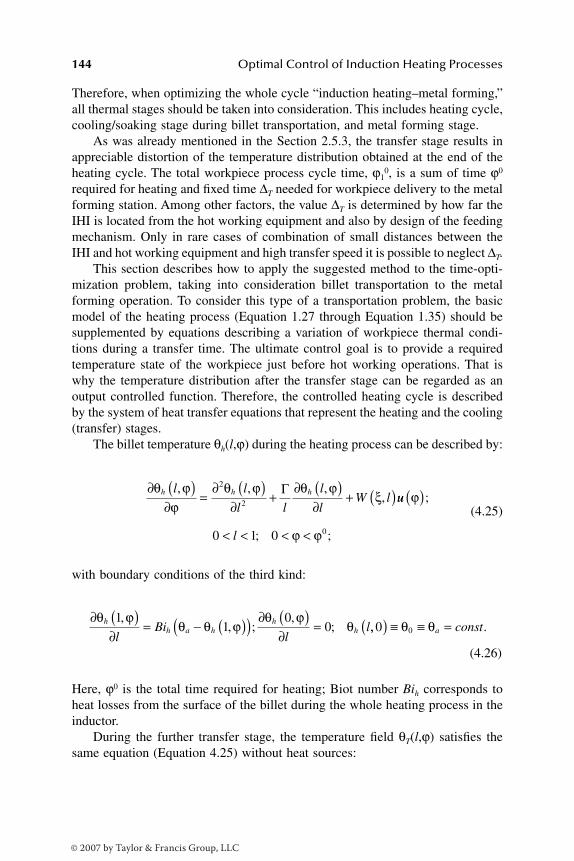
144 Optimal Control of Induction Heating Processes
Therefore, when optimizing the whole cycle “induction heating–metal forming,”all thermal stages should be taken into consideration. This includes heating cycle,cooling/soaking stage during billet transportation, and metal forming stage.
As was already mentioned in the Section 2.5.3, the transfer stage results inappreciable distortion of the temperature distribution obtained at the end of theheating cycle. The total workpiece process cycle time, ϕ1
0, is a sum of time ϕ0
required for heating and fixed time ∆T needed for workpiece delivery to the metalforming station. Among other factors, the value ∆T is determined by how far theIHI is located from the hot working equipment and also by design of the feedingmechanism. Only in rare cases of combination of small distances between theIHI and hot working equipment and high transfer speed it is possible to neglect ∆T.
This section describes how to apply the suggested method to the time-opti-mization problem, taking into consideration billet transportation to the metalforming operation. To consider this type of a transportation problem, the basicmodel of the heating process (Equation 1.27 through Equation 1.35) should besupplemented by equations describing a variation of workpiece thermal condi-tions during a transfer time. The ultimate control goal is to provide a requiredtemperature state of the workpiece just before hot working operations. That iswhy the temperature distribution after the transfer stage can be regarded as anoutput controlled function. Therefore, the controlled heating cycle is describedby the system of heat transfer equations that represent the heating and the cooling(transfer) stages.
The billet temperature θh(l,ϕ) during the heating process can be described by:
(4.25)
with boundary conditions of the third kind:
(4.26)
Here, ϕ0 is the total time required for heating; Biot number Bih corresponds toheat losses from the surface of the billet during the whole heating process in theinductor.
During the further transfer stage, the temperature field θT(l,ϕ) satisfies thesame equation (Equation 4.25) without heat sources:
∂ ( )∂
=∂ ( )
∂+
∂ ( )∂
+ ( )θ ϕϕ
θ ϕ θ ϕξh h hl l
l l
l
lW l
, , ,,
2
2
Γuu
l
ϕ
ϕ ϕ
( )
< < < <
;
; ;0 1 0 0
∂ ( )∂
= − ( )( ) ∂ ( )∂
=θ ϕ
θ θ ϕθ ϕ
θhh a h
hh
lBi
ll
11
00
,, ;
,; ,, .0 0( ) ≡ ≡ =θ θa const
DK6039_C004.fm Page 144 Thursday, June 8, 2006 12:34 PM
© 2007 by Taylor & Francis Group, LLC

Optimal Control of Static Induction Heating Processes 145
(4.27)
with boundary conditions
.
(4.28)
Time ∆T should be considered here as a total transportation time. Heat lossesduring the transfer stage can be estimated by the value BiT in Equation (4.28)that vastly increases in comparison with heat losses inside the induction coil (BiT
> Bih). This leads to intensive billet cooling during the transfer stage.Initial temperature distribution θT(l,ϕ0) at the beginning of the transfer stage
complies with final temperature distribution θh(l,ϕ0) at the end of the heatingstage. This fact, written in the form of equality in Equation (4.28), is imperativeto bind the workpiece temperature field during the heating stage to that duringthe transfer stage.
At the time ϕ = ϕ0 + ∆T , instead of Equation (2.25), the condition for therequired absolute accuracy of heating can be formulated as:
. (4.29)
The time-optimal control problem will be considered based upon the follow-ing assumptions:
1. Equation (4.25) through Equation (4.28) represent the heating process.2. Initial billet temperature distribution prior to the induction heating
stage is assumed to be uniform, and required temperature distributionis described by Equation (4.29).
3. Heating power u(ϕ) is chosen as a control input function and the controlconstraint set is given in the form of Equation (2.7).
4. The cost function can be estimated by the time-optimal criterion (Equa-tion 2.1).
The statement of the time-optimal control problem can be formulated as thefollowing. It is necessary to select this control function u(ϕ) = u*(ϕ) bounded bythe preassigned set in Equation (2.7) that provides steering the workpiece initialtemperature distribution to the desired temperature θ* with prescribed accuracyε (according to Equation 4.29) for the moment ϕ = ϕ0 + ∆T. The control functionu*(ϕ) should hold cost criterion at extremum value.
∂ ( )∂
=∂ ( )
∂+
∂ ( )∂
+ < <θ ϕ
ϕθ ϕ θ ϕT T Tl l
l l
l
ll
, , ,;
2
2 0 1Γ ϕϕ ϕ ϕ0 0< < + ∆T ;
∂ ( )∂
= − ( )( ) ∂ ( )∂
=θ ϕ
θ θ ϕθ ϕ
θTT a T
TT
lBi
ll
11
00
,, ;
,; ,, ,ϕ θ ϕ0 0( ) ≡ ( )h l
max ,,
*
lTl
∈[ ]+( ) − ≤
0 1
0θ ϕ θ ε∆
DK6039_C004.fm Page 145 Thursday, June 8, 2006 12:34 PM
© 2007 by Taylor & Francis Group, LLC

146 Optimal Control of Induction Heating Processes
Obviously, in the case of fixed value of ∆T , the process of billet heating tothe certain a priori unknown temperature distribution θh(l,ϕ0) (complying withθT(l,ϕ0)) must be time optimal. In this case, the total process time proves to beminimal.
Similarly to Section 2.8, it is possible to prove mathematically1 that, withregard to the considered models, the time-optimal control algorithm consists ofalternating stages of heating with maximum power u ≡ Umax (heat ON) andsubsequent soaking/cooling under power u ≡ 0 (heat OFF) cycles. Consequently,optimal control u*(ϕ) can be written in the form of Equation (2.27) (Figure 2.8).
Let us consider the transfer stage of known fixed duration ∆T as an additionallast stage of the heating cycle under u(ϕ) ≡ 0. Optimal control u**(ϕ) of the wholeheating cycle described by the system of Equation (4.25) through Equation (4.28)can be written in the same form (Equation 2.27). However, duration of the transferstage and billet cooling rate are beyond the control — i.e., control stages of theheating cycle are supplemented by the uncontrollable transfer stage of fixedduration ∆T. This leads to a number of the essential features in contrast to thecontrol function u*(ϕ) when the billet was inside the induction coil.
Total number N1 of u**(ϕ) stages always proves to be even because, in thelast interval, the control u**(ϕ) is equal to zero (during billet transfer), and on thefirst stage it is always equal to Umax. The last control stage could be longer thanthe transfer stage. In this case, the remaining time of this stage takes place whenthe billet is inside the inductor section that has no power (so-called passivesection). Therefore, the number N of u*(ϕ) stages proves to be equal to N1. If theduration of the last control stage coincides with the transfer stage, then it ispossible to assume the following expression: N = N1 – 1.
Let us consider as an example a single-stage heating with u*(ϕ) ≡ Umax (N =1). The control u**(ϕ) consists of two stages (N1 = N + 1) with the no-powersecond interval realized under u(ϕ) = 0 during workpiece transfer (Figure 4.14).The two-stage heating cycle (N = 2) means that, after heating under maximumpower, the next interval of temperature soaking takes place inside the inductioncoil. The following mandatory transfer stage only prolongs duration of the second(heat OFF) interval of the control function u**(ϕ) and N1 remains equal to N(Figure 4.15).
FIGURE 4.14 Time-optimal control with consideration of the transfer stage in the caseof N = 1, N1 = 2, αT = 1.
0
Umax
u∗∗(ϕ)
∆10 ∆T
ϕϕ0
DK6039_C004.fm Page 146 Thursday, June 8, 2006 12:34 PM
© 2007 by Taylor & Francis Group, LLC
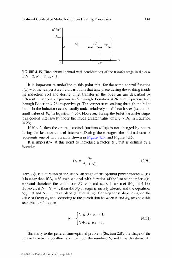
Optimal Control of Static Induction Heating Processes 147
It is important to underline at this point that, for the same control functionu(ϕ) = 0, the temperature field variations that take place during the soaking insidethe induction coil and during billet transfer in the open air are described bydifferent equations (Equation 4.25 through Equation 4.26 and Equation 4.27through Equation 4.28, respectively). The temperature soaking through the billetthat is in the inductor occurs usually under relatively small heat losses (i.e., undersmall value of Bih in Equation 4.26). However, during the billet’s transfer stage,it is cooled intensively under the much greater value of BiT > Bih in Equation(4.28).
If N > 2, then the optimal control function u**(ϕ) is not changed by natureduring the last two control intervals. During these stages, the optimal controlrepresents one of two variants shown in Figure 4.14 and Figure 4.15.
It is imperative at this point to introduce a factor, αT, that is defined by aformula:
. (4.30)
Here, ∆0N1
is a duration of the last N1-th stage of the optimal power control u*(ϕ).It is clear that, if N1 = N, then we deal with duration of the last stage under u(ϕ)= 0 and therefore the conditions ∆0
N1> 0 and αT < 1 are met (Figure 4.15).
However, if N = N1 – 1, then the N1-th stage is merely absent, and the equalities∆0
N1= 0 and αT = 1 take place (Figure 4.14). Consequently, depending on the
value of factor αT and according to the correlation between N and N1, two possiblescenarios could exist:
(4.31)
Similarly to the general time-optimal problem (Section 2.8), the shape of theoptimal control algorithm is known, but the number, N, and time durations, ∆1,
FIGURE 4.15 Time-optimal control with consideration of the transfer stage in the caseof N = 2, N1 = 2, αT < 1.
0
Umax
u∗∗(ϕ)
∆20∆
10 ∆T
ϕϕ0
αTT
T N
=+∆
∆ ∆ 10
NN if
N if
T
T
1
0 1
1 1=
< <
+ =
, ;
, .
α
α
DK6039_C004.fm Page 147 Thursday, June 8, 2006 12:34 PM
© 2007 by Taylor & Francis Group, LLC
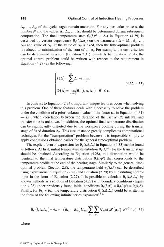
148 Optimal Control of Induction Heating Processes
∆2, …, ∆N, of the cycle stages remain uncertain. For any particular process, thenumber N and the values ∆1, ∆2, …, ∆N should be determined during subsequentcomputation. The final temperature state θT(l,ϕ0 + ∆T) in Equation (4.29) isdescribed by certain dependency θT(l,∆,∆T) on the parameters ∆ = (∆1, ∆2, …,∆N) and value of ∆T . If the value of ∆T is fixed, then the time-optimal problemis reduced to minimization of the sum of all ∆i. For example, the cost criterioncan be determined as a sum (Equation 2.31). Similarly to Equation (2.34), theoptimal control problem could be written with respect to the requirement inEquation (4.29) as the following:
(4.32, 4.33)
In contrast to Equation (2.34), important unique features occur when solvingthis problem. One of these features deals with a necessity to solve the problemunder the condition of a priori unknown value of the factor αT in Equation (4.31)— i.e., when correlation between the duration of the last u**(ϕ) interval andtransfer time is unknown. In addition, the optimal final temperature distributioncan be significantly distorted due to the workpiece cooling during the transferstage of fixed duration ∆T . This circumstance greatly complicates computationaltechniques for the “transportation” problem because it is impossible simply toapply conclusions obtained earlier for the general time-optimal problem.
The explicit form of expression for θT (l,∆,∆T) in Equation (4.33) can be foundas follows. At first, initial temperature distribution θT(l,ϕ0) for the transfer stageshould be obtained. According to Equation (4.28), this distribution would beidentical to the final temperature distribution θh(l,ϕ0) that corresponds to thetemperature profile at the end of the heating stage. Similarly to the general time-optimal problem (Section 2.8), the temperature field θh(l,ϕ0) can be describedusing expressions in Equation (2.28) and Equation (2.29) by substituting controlinput in the form of Equation (2.27). It is possible to calculate θT (l,∆,∆T) byknown methods as a solution of Equation (4.27) with boundary conditions (Equa-tion 4.28) under previously found initial conditions θT(l,ϕ0) = θh(l,ϕ0) = θh(l,∆).Finally, for BiT ≠ Bih, the temperature distribution θT(l,∆,∆T) could be written inthe form of the following infinite series expansion1,2,8:
,(4.34)
where
I
l
i
i
N
lT T
∆ ∆
Φ ∆ ∆ ∆
∆( ) = →
( ) = ( )=
∈[ ]
∑1
0 1
min;
max , ,,
θ −− ≤
θ ε* .
θ θT T T h ns
ns
nl Bi Bi U N M, , max∆ ∆( ) = + −( )=
∞
=
∞
∑∑0
11
4 KK l ess Tµ µ( ) ⋅ − 2∆
DK6039_C004.fm Page 148 Thursday, June 8, 2006 12:34 PM
© 2007 by Taylor & Francis Group, LLC

Optimal Control of Static Induction Heating Processes 149
(4.35)
, (4.36)
and µn and µs represent corresponding roots of the equations:
BihK(µ) – µK1(µ) = 0; BiTK(µ) – µK1(µ) = 0. (4.37)
Thus, this optimal control problem is reduced to solution of the mathematicalprogramming problem (Equation 4.32 through Equation 4.37), which should beconsidered as a particular case of the general problem (Equation 3.38).
4.2.2 COMPUTATIONAL TECHNIQUE FOR THE “TRANSPORTATION” PROBLEM OF TIME-OPTIMAL HEATING
The basic properties (Equation 3.39 and Equation 3.40) remain valid for the finaltemperature distribution θT (l,∆,∆T) in the transportation problem of time-optimalheating (see conclusions made in Section 3.7). The proposed engineering tech-nique is based on these universal features as they are used in the course ofcomputational procedure.
It is important to notice that the fixed value ∆T is not included in the set ofsought parameters. Because N1 is always an even value, the appropriate inequal-ities sequence (Equation 3.41) contains only minimax temperature deviations
with even indices:
. (4.38)
The sign “~” is used to indicate a minimax temperature deviation consideredin the class of “general” control inputs u**(ϕ) with N1 intervals. It is possible toprove1 that in this case the basic relation in Equation (3.3) holds true aftersubstituting N1 and εmin
(s) instead of N and , respectively:
. (4.39)
Number N1 of u**(ϕ) constancy intervals depends on the place of ε in the sequencein Equation (4.38) and can be defined according to Equation (4.39).
N W Bi Bi Bins n s s T T n h= ( ) + + −( )( ) ⋅ + + −ξ µ µ µ2 2 2 2 21 1Γ ΓΓ( )( ) ⋅
−( ) ⋅ ( ) ⋅ ( )−
Bi
K K
h
s n s nµ µ µ µ2 21,
Mnr
r
N
n m
m r
N
= −( ) − −
+
= =∑ ∑1 1
1
1
2exp µ ∆
εmin*, ,k k N( ) = 1
ε ε ε εmin min min inf...*
2 4 0( ) ( ) ( )> > > = >N
εmin( )s
N S for all S S1
1= ≤ <( ) −( )ε ε ε ε: min min
DK6039_C004.fm Page 149 Thursday, June 8, 2006 12:34 PM
© 2007 by Taylor & Francis Group, LLC

150 Optimal Control of Induction Heating Processes
On the basis of the universal properties in Equation (3.39) and Equation(3.40), the particular temperature profile of final temperature distribution shouldbe revealed depending on the given time of transfer stage that represents thespecifics of the transportation time-optimal control problem.
It is important to note that the previously mentioned deal with the case of αT
= 1. It is easy to understand that, under αT < 1, all basic rules and properties ofthe temperature profile stated in Chapter 3 for time-optimal problem (with ∆T =0) remain the same for the considered case of ∆T > 0. Obviously, if αT = 1, thenthe sum 0∆N1
+ ∆T represents total duration of the last interval of control functionu*(ϕ) (Figure 4.15). Therefore, it turns out that duration of the last interval ofu*(ϕ) can be changed by varying the value 0∆N1
> 0. This means that the lastinterval time is under control as well as all intervals . All constancyintervals of control function u**(ϕ) can be chosen freely as well as in the generaltime-optimal problem.
Conclusions regarding dependency of number N on ε prove to be the same.The shape of the curve that represents temperature distribution at the end of theoptimal process will also be the same as in the general OCP. At the same time,only the case of αT = 1 (under 0∆N1
= 0 [Figure 4.14]) should be considered asan exception because duration of the last N1-th interval of control u**(ϕ) becomesfixed and equal to ∆T. Essentially, the number of sought parameters decreases byone. This is the main reason that the properties of final temperature distributionare changed under αT = 1.
If the value of the factor αT in Equation (4.30) is unknown a priori, then thefollowing solution algorithm is suggested for the transportation time-optimalcontrol problem (Figure 4.16):
1. The first term, , of the inequalities series (Equation 4.38) representsthe best heating accuracy for the class of two-stage control inputsu**(ϕ). Obviously, depends on the value ∆T . The accuracy canbe reached using control inputs with different values ∆T for αT = 1 orαT < 1 (Figure 4.14 and Figure 4.15). It is clear that condition αT = 1is met if the value ∆T is appreciably large and billet soaking inside theinduction coil becomes unnecessary because sufficient temperatureequalization takes place during the transfer stage. On the other hand,the condition αT < 1 is true if the value ∆T is substantially small, leadingto too short duration of this stage for providing required temperatureequalization. Taking this fact into consideration, it is possible to choosecertain minimum (unknown a priori) value ∆T = ∆T2
* from all ∆T valuesfor which αT = 1 (Figure 4.17). This value will correspond to a certainvalue of (∆T2).* The problem in Equation (4.32) through Equation (4.37) can be solvedassuming that required heating accuracy complies with (∆T2)
* andgiven transportation time is equal to ∆T2.* Let us consider two valuesof ∆T : ∆T = ∆T2
* and ∆T = ∆T2* – δ∆T , where δ∆T > 0 is a small enough
value.
∆i i N0 1, ,=
εmin( )2
εmin( )2 εmin
( )2
εmin( )2
εmin( )2
DK6039_C004.fm Page 150 Thursday, June 8, 2006 12:34 PM
© 2007 by Taylor & Francis Group, LLC
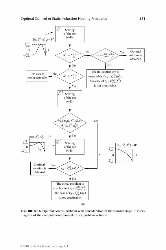
Optimal Control of Static Induction Heating Processes 151
FIGURE 4.16 Optimal control problem with consideration of the transfer stage. a: Blockdiagram of the computational procedure for problem solution.
(a)
Solving
of the set
(4.40) θ(l, ∆
10, ∆∗
T2) − θ∗
max θT(l, ∆10, ∆0
T) >
θT(0, ∆10, ∆°
T)?
∆T0 = ∆∗
T2?
∆T0 > ∆∗
T2?
Solving
of the set
(4.42)
Solving
of the set
(4.41)
Optimal
solution is
obtained
Optimal
solution is
obtained
Yes
No
No
Yes
Yes
Yes
1°
Yes 1 0 l
1 0 l le2
1
2°
This case is
not practicable
No
No
No
2°
εmin(2) ~
−εmin(2) ~
θ(l, ∆10, ∆0
T) − θ∗
εmin(2) ~
−εmin(2) ~
0 l
θ(l, ∆10, ∆0
T) − θ∗
εmin(2) ~
−εmin(2) ~
The initial problem is
unsolvable if ε0 < εmin(∆T0
).
The case of ε0 > εmin(∆T0
)
is not practicable.
~(2)
~(2)
The initial problem is
unsolvable if ε0 < εmin(∆T0
).
The case of ε0 > εmin(∆T0
)
is not practicable.
~(2)
~(2)
ε0 = εmin(∆T0
)?~(2)
ε0 = εmin(∆T° )?~(2)
DK6039_C004.fm Page 151 Thursday, June 8, 2006 12:34 PM
© 2007 by Taylor & Francis Group, LLC
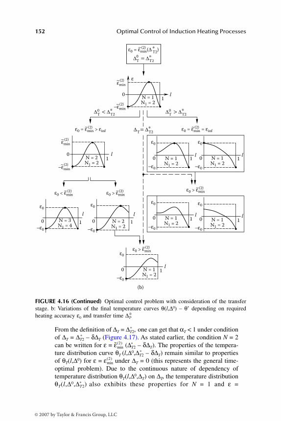
152 Optimal Control of Induction Heating Processes
From the definition of ∆T = ∆T2,* one can get that αT < 1 under conditionof ∆T = ∆T2
* – δ∆T (Figure 4.17). As stated earlier, the condition N = 2can be written for ε = (∆T2
* – δ∆T). The properties of the tempera-ture distribution curve θT (l,∆0,∆T2
* – δ∆T) remain similar to propertiesof θT(l,∆0) for ε = under ∆T = 0 (this represents the general time-optimal problem). Due to the continuous nature of dependency oftemperature distribution θT(l,∆0,∆T) on ∆T, the temperature distributionθT(l,∆0,∆T2)* also exhibits these properties for N = 1 and ε =
FIGURE 4.16 (Continued) Optimal control problem with consideration of the transferstage. b: Variations of the final temperature curves θ(l,∆0) – θ* depending on requiredheating accuracy ε0 and transfer time ∆T.
0
(b)
εmin(2)~
−εmin(2)~
∆T0 = ∆∗
T2
ε0 = εmin(∆∗T2
)~(2)
∆T = ∆∗
T2
∆T0 < ∆∗
T2∆
T0 > ∆∗
T2
ε0 = εmin > εinf~(2)
ε0 < εmin~(2) ε0 > εmin
~(2)
ε0 > εmin~(2)
ε0 > εmin~(2)
ε0 = εmin = εinf~(2)
0
εmin(2)~
−εmin(2)~
0
l1
l1
l1
N = 1N1 = 2
N = 2N1 = 2
N = 3N1 = 4
ε
ε0
0
−ε0
l1
l1
l1
l1N = 2
N1 = 2
N = 1N1 = 2
N = 1N1 = 2
N = 1N1 = 2
ε0
0
−ε0
ε0
0
−ε0
ε0
0
−ε0
ε0
0
−ε0
l1
l1N = 1
N1 = 2N = 1N1 = 2
ε0
0
−ε0
ε0
0
−ε0
εmin( )2
εmin( )2
DK6039_C004.fm Page 152 Thursday, June 8, 2006 12:34 PM
© 2007 by Taylor & Francis Group, LLC
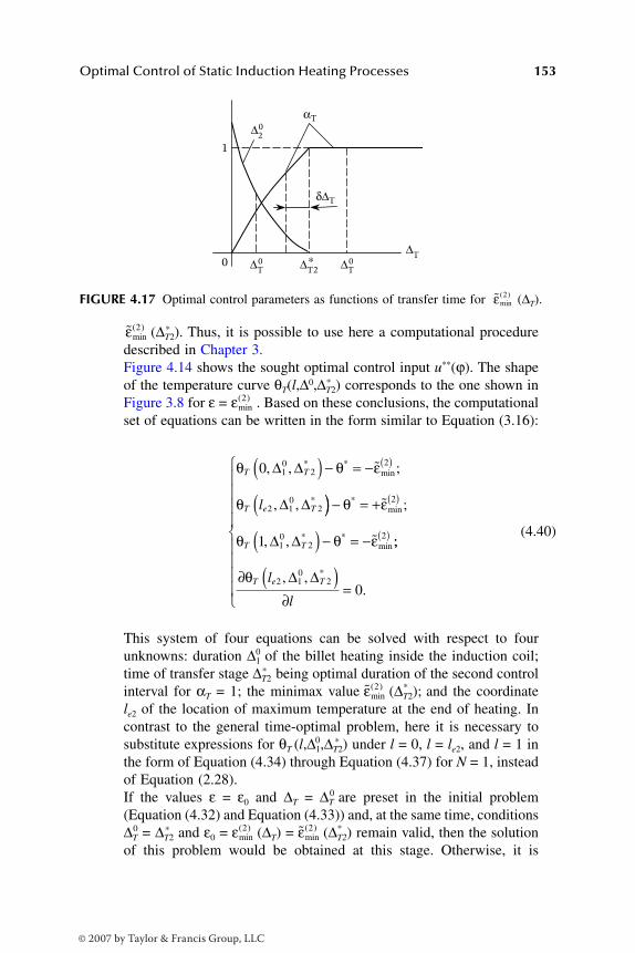
Optimal Control of Static Induction Heating Processes 153
(∆T2).* Thus, it is possible to use here a computational proceduredescribed in Chapter 3.Figure 4.14 shows the sought optimal control input u**(ϕ). The shapeof the temperature curve θT(l,∆0,∆T2)* corresponds to the one shown inFigure 3.8 for ε = . Based on these conclusions, the computationalset of equations can be written in the form similar to Equation (3.16):
(4.40)
This system of four equations can be solved with respect to fourunknowns: duration ∆1
0 of the billet heating inside the induction coil;time of transfer stage ∆T2
* being optimal duration of the second controlinterval for αT = 1; the minimax value (∆T2);
* and the coordinatele2 of the location of maximum temperature at the end of heating. Incontrast to the general time-optimal problem, here it is necessary tosubstitute expressions for 0θT (l,∆1,∆T2)* under l = 0, l = le2, and l = 1 inthe form of Equation (4.34) through Equation (4.37) for N = 1, insteadof Equation (2.28).If the values ε = ε0 and ∆T = ∆T
0 are preset in the initial problem(Equation (4.32) and Equation (4.33)) and, at the same time, conditions∆T
0 = ∆T2* and ε0 = (∆T) = (∆T2)
* remain valid, then the solutionof this problem would be obtained at this stage. Otherwise, it is
FIGURE 4.17 Optimal control parameters as functions of transfer time for (∆T).
1
0 ∆T0 ∆
T0
∆20
∆T
αT
δ∆T
∆T∗
2
εmin( )2
εmin( )2
εmin( )2
θ θ ε
θ
T T
T e Tl
0 10
22
2 10
2
, , ;
, ,
* *min
*
∆ ∆
∆ ∆
( ) − = −
(
( )
)) − = +
( ) − = −
( )
( )
θ ε
θ θ ε
*min
* *min
;
, ,
2
10
221T T∆ ∆ ;;
, ,.
*∂ ( )∂
=
θT e Tl
l
2 10
20
∆ ∆
εmin( )2
εmin( )2 εmin
( )2
DK6039_C004.fm Page 153 Thursday, June 8, 2006 12:34 PM
© 2007 by Taylor & Francis Group, LLC
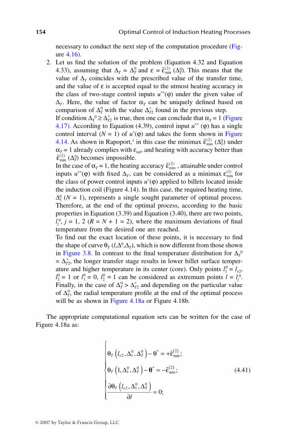
154 Optimal Control of Induction Heating Processes
necessary to conduct the next step of the computation procedure (Fig-ure 4.16).
2. Let us find the solution of the problem (Equation 4.32 and Equation4.33), assuming that ∆T = ∆T
0 and ε = (∆T).0 This means that thevalue of ∆T coincides with the prescribed value of the transfer time,and the value of ε is accepted equal to the utmost heating accuracy inthe class of two-stage control inputs u**(ϕ) under the given value of∆T . Here, the value of factor αT can be uniquely defined based oncomparison of ∆T
0 with the value ∆T2* found in the previous step.
If condition ∆T0 ≥ ∆T2
* is true, then one can conclude that αT = 1 (Figure4.17). According to Equation (4.39), control input u** (ϕ) has a singlecontrol interval (N = 1) of u*(ϕ) and takes the form shown in Figure4.14. As shown in Rapoport,1 in this case the minimax (∆T)0 underαT = 1 already complies with εinf, and heating with accuracy better than
(∆T)0 becomes impossible.In the case of αT = 1, the heating accuracy , attainable under controlinputs u**(ϕ) with fixed ∆T , can be considered as a minimax forthe class of power control inputs u*(ϕ) applied to billets located insidethe induction coil (Figure 4.14). In this case, the required heating time,∆1
0 (N = 1), represents a single sought parameter of optimal process.Therefore, at the end of the optimal process, according to the basicproperties in Equation (3.39) and Equation (3.40), there are two points,lj
0, j = 1, 2 (R = N + 1 = 2), where the maximum deviations of finaltemperature from the desired one are reached.To find out the exact location of these points, it is necessary to findthe shape of curve θT (l,∆0,∆T), which is now different from those shownin Figure 3.8. In contrast to the final temperature distribution for ∆T
0
= ∆T2,* the longer transfer stage results in lower billet surface temper-ature and higher temperature in its center (core). Only points l1
0 = le2,l2
0 = 1 or l10 = 0, l2
0 = 1 can be considered as extremum points l = lj0.
Finally, in the case of ∆T0 > ∆T2
* and depending on the particular valueof ∆T,0 the radial temperature profile at the end of the optimal processwill be as shown in Figure 4.18a or Figure 4.18b.
The appropriate computational equation sets can be written for the case ofFigure 4.18a as:
(4.41)
εmin( )2
εmin( )2
εmin( )2
εmin( )2
εmin( )1
θ θ ε
θ
T e T
T T
l 2 10 0 2
10 01
, , ;
, ,
*min∆ ∆
∆ ∆
( ) − = +
( ) −
( )
θθ ε
θ
*min;
, ,;
= −
∂ ( )∂
=
( ) 2
2 10 0
0T e Tl
l
∆ ∆
DK6039_C004.fm Page 154 Thursday, June 8, 2006 12:34 PM
© 2007 by Taylor & Francis Group, LLC
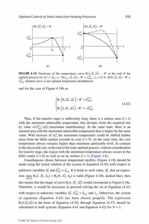
Optimal Control of Static Induction Heating Processes 155
and for the case of Figure 4.18b as:
(4.42)
Thus, if the transfer stage is sufficiently long, there is a surface area (l = 1)with the minimum admissible temperature that deviates from the required oneby value of (∆T)
0 (maximum underheating). At the same time, there is aninternal area with the maximum admissible temperature that is higher by the samevalue. With increase of ∆T,0 the maximum temperature could be shifted furtheraway from the billet surface towards its core (l = 0). At the same time, the coretemperature always remains higher than minimum admissible level. In contrastto the discussed case, at the end of the time-optimal process, without considerationfor transfer stage, the region with the minimum temperature always occurs in thebillet center (l = 0) as well as on its surface (l = 1) (Figure 3.8).
Unambiguous choice between temperature profiles (Figure 4.18) should bemade using the tested solution of the system in Equation (4.42) with respect to
unknown variables ∆10 and = εinf . If it leads to such value, ∆1,
0 that an expres-
sion θT(l, ∆1,0 ∆T) > θT(0, ∆1,
0 ∆T) is valid (Figure 4.18b, dashed line), then
this means that the shape of curve θT(l, ∆1,0 ∆T)
0 would correspond to Figure 4.18a.Therefore, it would be necessary to proceed solving the set in Equation (4.41)
with respect to unknown variables ∆1,0 = εinf, and le2. Otherwise, the system
of equations (Equation 4.42) has been chosen properly. The expressionθT(l,∆1,∆T)0 in0 the form of Equation (4.34) through Equation (4.37) should besubstituted in both systems (Equation 4.41 and Equation 4.42) for N = 1.
FIGURE 4.18 Variations of the temperature curve θ – θ* at the end of theoptimal process for ∆T
0 > *∆T2: a – θ – θ* = , le2 > 0; b –θ – θ* = (dashed curve is not optimal temperature distribution).
(a) (b)
0 1l
le20 1
θ(l, ∆10, ∆0
T) − θ∗ θ(l, ∆
10, ∆0
T) − θ∗
εmin(2)~
−εmin(2)~
l
εmin(2)~
−εmin(2)~
l ∆10 ∆T
0, ,( )le2 ∆1
0 ∆T0, ,( ) εmin
2( ) 0 ∆10 ∆T
0, ,( )εmin
2( )
θ θ ε
θ θ
T T
T T
0
1
10 0 2
10 0
, , ;
, ,
*min
*
∆ ∆
∆ ∆
( ) − =
( ) − =
( )
−−
( )εmin .2
εmin( )2
εmin( )2
max,l∈[ ]0 1
εmin( )2
DK6039_C004.fm Page 155 Thursday, June 8, 2006 12:34 PM
© 2007 by Taylor & Francis Group, LLC
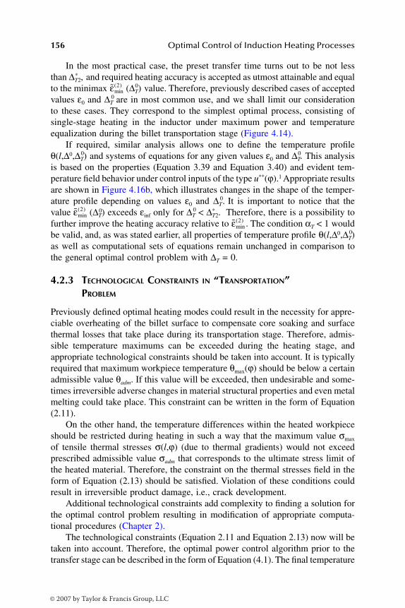
156 Optimal Control of Induction Heating Processes
In the most practical case, the preset transfer time turns out to be not lessthan ∆T2,* and required heating accuracy is accepted as utmost attainable and equalto the minimax (∆T)
0 value. Therefore, previously described cases of acceptedvalues ε0 and ∆T
0 are in most common use, and we shall limit our considerationto these cases. They correspond to the simplest optimal process, consisting ofsingle-stage heating in the inductor under maximum power and temperatureequalization during the billet transportation stage (Figure 4.14).
If required, similar analysis allows one to define the temperature profileθ(l,∆0,∆T)
0 and systems of equations for any given values ε0 and ∆T.0 This analysis
is based on the properties (Equation 3.39 and Equation 3.40) and evident tem-perature field behavior under control inputs of the type u**(ϕ).1 Appropriate resultsare shown in Figure 4.16b, which illustrates changes in the shape of the temper-ature profile depending on values ε0 and ∆T.0 It is important to notice that thevalue (∆T)0 exceeds εinf only for ∆T
0 < ∆T2.* Therefore, there is a possibility tofurther improve the heating accuracy relative to . The condition αT < 1 wouldbe valid, and, as was stated earlier, all properties of temperature profile 0θ(l,∆0,∆T)as well as computational sets of equations remain unchanged in comparison tothe general optimal control problem with ∆T = 0.
4.2.3 TECHNOLOGICAL CONSTRAINTS IN “TRANSPORTATION” PROBLEM
Previously defined optimal heating modes could result in the necessity for appre-ciable overheating of the billet surface to compensate core soaking and surfacethermal losses that take place during its transportation stage. Therefore, admis-sible temperature maximums can be exceeded during the heating stage, andappropriate technological constraints should be taken into account. It is typicallyrequired that maximum workpiece temperature θmax(ϕ) should be below a certainadmissible value θadm. If this value will be exceeded, then undesirable and some-times irreversible adverse changes in material structural properties and even metalmelting could take place. This constraint can be written in the form of Equation(2.11).
On the other hand, the temperature differences within the heated workpieceshould be restricted during heating in such a way that the maximum value σmax
of tensile thermal stresses σ(l,ϕ) (due to thermal gradients) would not exceedprescribed admissible value σadm that corresponds to the ultimate stress limit ofthe heated material. Therefore, the constraint on the thermal stresses field in theform of Equation (2.13) should be satisfied. Violation of these conditions couldresult in irreversible product damage, i.e., crack development.
Additional technological constraints add complexity to finding a solution forthe optimal control problem resulting in modification of appropriate computa-tional procedures (Chapter 2).
The technological constraints (Equation 2.11 and Equation 2.13) now will betaken into account. Therefore, the optimal power control algorithm prior to thetransfer stage can be described in the form of Equation (4.1). The final temperature
εmin( )2
εmin( )2
εmin( )2
DK6039_C004.fm Page 156 Thursday, June 8, 2006 12:34 PM
© 2007 by Taylor & Francis Group, LLC

Optimal Control of Static Induction Heating Processes 157
distribution θT(l,∆0,∆T)0 at the end of this stage is described by Expression (4.34),
in which it is necessary to replace Mn to Cn in the form of Equation (4.16).If condition ∆T
0 < ∆T2* holds true and Expression (4.17) is valid for given
heating accuracy, then the optimal computational technique described in Section4.1 remains unchanged for the transportation problem. The foregoing conclusionfollows from the fact that lengths of all u**(ϕ) intervals remain under controlwhen αT becomes less than 1. This conclusion can be extended to the case of 0∆T
= *∆T2. Here, ∆T2* makes the same sense as in Section 4.2.2. The difference lies in
the fact that the earlier obtained expression for final temperature distributionθT(l,∆0,∆T)
0 should be substituted into computational sets of equations. Noticeabledistinctions emerge only when these conditions are not met.
1. Let us first consider the case when condition ε > θadm – θ* holds true(Section 4.1.3). Because temperature maximum, which is limited dur-ing the whole heating process by value θadm, can only decrease duringthe transfer stage, then only negative admissible deviations of finaltemperature from a required one could be reached. These deviationsare equal to –ε.Let us assume that ε = (∆T).
0 If technological constraints will betaken into account, the shape of temperature distribution 0θT(l,∆0,∆T)typically remains the same. Then the area with the minimum temper-atures can be reached only at two points: l = 0 and l = 1 for N = 1 (ifαT = 1) or N = 2 (if αT < 1) (Figure 4.16b). At the same time, if αT <1 and N = 2, then the value ε = in the class of controls u**(ϕ) canbe considered as in the class of u*(ϕ) for fixed value ∆T . In thatcase, according to Equation (3.39) and Equation (3.40), three pointswith minimum temperature θ∗ – should exist. Therefore the condition αT < 1 is impossible and αT = 1, N = 1 (Figure4.14). Similarly to other cases for αT = 1 (Section 4.2.2), the condition
= εinf would hold true. Minimax can be treated as a val-ue in the class of controls u*(ϕ) for the same fixed value ∆T. As a
FIGURE 4.19 Time-optimal transportation problem with technological restraints for ε = > θadm – θ* and ∆1
0 > ϕθ. a: optimal control; b: final temperature profile.
εmin( )2
εmin( )2
εmin( )2
εmin( )2
εmin( )2 εmin
( )2
εmin( )1
(a) (b)
0
0
u∗∗(ϕ)
Umax
1l
θ(l, ∆10, ∆0
T) − θ∗
θadm − θ∗εmin
(2)~
−εmin(2)~ϕσ ϕθ
∆10 ∆
T0
ϕ
εmin2( )
DK6039_C004.fm Page 157 Thursday, June 8, 2006 12:34 PM
© 2007 by Taylor & Francis Group, LLC

158 Optimal Control of Induction Heating Processes
result, in practice an optimal process with ultimately allowable devia-tion εinf > θadm – θ* can be applied relatively easily. It consists of twostages. The first one is heating with maximum power under constrainedcontrol, thermal stresses, and maximum temperature according to algo-rithm (Equation 4.1). The second stage is workpiece transfer duringfixed time ∆T
0 (Figure 4.19a).According to Equation (3.39) and Equation (3.40), at the end of optimalprocess the minimum temperatures θ∗ – should be reached at twopoints: in the center, l = 0, and on the surface, l = 1, of the billet (Figure4.19b; compare to Figure 4.9). An appropriate set of equations takesthe following form:
(4.43)
This set can be solved with respect to ∆10 and .
If transfer stage duration ∆T0 is sufficiently long, only the second equal-
ity in Equation (4.43) can be met. This is so in our case because onlya single point of minimum temperature exists on the billet surface(Figure 4.20). Therefore, one can obtain that R = 1 for ε = εmin
(N) inEquation (3.39) and Equation (3.40). This means that optimal controlproves to be completely determined a priori and there are no unknownparameters (i.e., N = 0!). This conclusion holds true for ϕθ = ∆1
0 inEquation (4.1) — i.e., when the transfer stage begins at the momentof obtaining maximum admissible temperature θadm.
FIGURE 4.20 Variations of final temperature profile for the time-optimal transportationproblem with technological constraints: ε = (∆T)
0 > θadm – θ* and ∆10 = ϕθ.
εmin( )2
θ θ ε
θ θ
T T
T T
0
1
10 0 2
10 0
, , ;
, ,
*min
*
∆ ∆
∆ ∆
( ) − = −
( ) −
( )
== −
( )εmin .2
εmin( )2
(a) (b)
0 1l l
0 1
θT(l, ∆10, ∆0
T) − θ∗
θadm − θ∗εmin
(2)~
−εmin(2)~
θT(l, ∆10, ∆0
T) − θ∗
θadm − θ∗εmin
(2)~
−εmin(2)~
εmin2( )
DK6039_C004.fm Page 158 Thursday, June 8, 2006 12:34 PM
© 2007 by Taylor & Francis Group, LLC
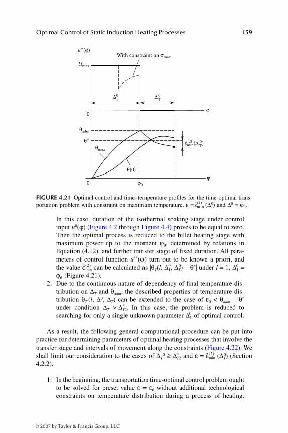
Optimal Control of Static Induction Heating Processes 159
In this case, duration of the isothermal soaking stage under controlinput uθ(ϕ) (Figure 4.2 through Figure 4.4) proves to be equal to zero.Then the optimal process is reduced to the billet heating stage withmaximum power up to the moment ϕθ, determined by relations inEquation (4.12), and further transfer stage of fixed duration. All para-meters of control function u**(ϕ) turn out to be known a priori, andthe value can be calculated as |θT(l, ∆1,
0 ∆T)0 – θ*| under l = 1, 0∆1 =
ϕθ (Figure 4.21). 2. Due to the continuous nature of dependency of final temperature dis-
tribution on ∆T and θadm, the described properties of temperature dis-tribution θT (l, ∆0, ∆T) can be extended to the case of ε0 < θadm – θ*
under condition ∆T > *∆T2. In this case, the problem is reduced tosearching for only a single unknown parameter ∆1
0 of optimal control.
As a result, the following general computational procedure can be put intopractice for determining parameters of optimal heating processes that involve thetransfer stage and intervals of movement along the constraints (Figure 4.22). Weshall limit our consideration to the cases of ∆T
0 ≥ ∆T2* and ε = (∆T)0 (Section
4.2.2).
1. In the beginning, the transportation time-optimal control problem oughtto be solved for preset value ε = ε0 without additional technologicalconstraints on temperature distribution during a process of heating.
FIGURE 4.21 Optimal control and time–temperature profiles for the time-optimal trans-portation problem with constraint on maximum temperature. ε = (∆T)
0 and ∆10 = ϕθ.
u∗(ϕ)
Umax
0
With constraint on σmax
0
θadm
θmax
θ(0)
θ∗
∆10 ∆
T0
ϕ
ϕϕθ
εmin(∆T0)∼(2)
εmin2( )
εmin( )2
εmin( )2
DK6039_C004.fm Page 159 Thursday, June 8, 2006 12:34 PM
© 2007 by Taylor & Francis Group, LLC

160 Optimal Control of Induction Heating Processes
FIGURE 4.22 Time-optimal transportation problem with constraints on θmax and σmax. a:Block diagram of the computational procedure for problem solution.
(a)
Solving of the set (4.44)
Solution of “transportation”
problem without technological
constraints (Section 4.2.2)
Computation of optimal
process for ∆T = 0, ε = εmin(Section 4.1.3)
Optimal
solution is
obtained
Optimal
solution is
obtained
Optimal
solution is
obtained
No
l N = 1 N1 = 2
0
θadm − θ∗
~(2) −εmin
~(2) εmin
l
l
l
N = 1 N1 = 2
0
0
θadm − θ∗
θadm − θ∗
~(2) εmin
~(2) −εmin
0
θadm − θ∗
~(2) −εmin
~(2) −εmin
l N = 1 N1 = 2
0
θadm − θ∗
~(2) −εmin
~(2) εmin
(1)
(1)
εmin > εinf ?
No
Yes
Yes
Yes
Yes
2°
Solving of the set (4.40)
Solving of the set (4.43)
Yes
Yes Solving of the second
equation in (4.43)
for ∆10 = ϕθ
No
No
1
1
1
1
1
No
∆T0 = ∆
T2
∆T0 > ∆
T∗
2 ?
∆T0 < ∆
T2
∆T0 = ∆
T2
Optimal solution
is obtained
Yes
This case is not
practicable
No
No
3°
4°
4°
4°, 5°
1°
σmax(ϕ) ≥ σadm ?and (or)
θmax(ϕ) ≥ θadm?
ε
ε0 = εmin(∆T0 ) ?
(2) ~
The initial problem is
unsolvable if ε0 < εmin(∆T0
).
The case of ε0 > εmin(∆T0
)
is not practicable.
~(2)
~(2)
∗∗∗∗
∗
DK6039_C004.fm Page 160 Thursday, June 8, 2006 12:34 PM
© 2007 by Taylor & Francis Group, LLC
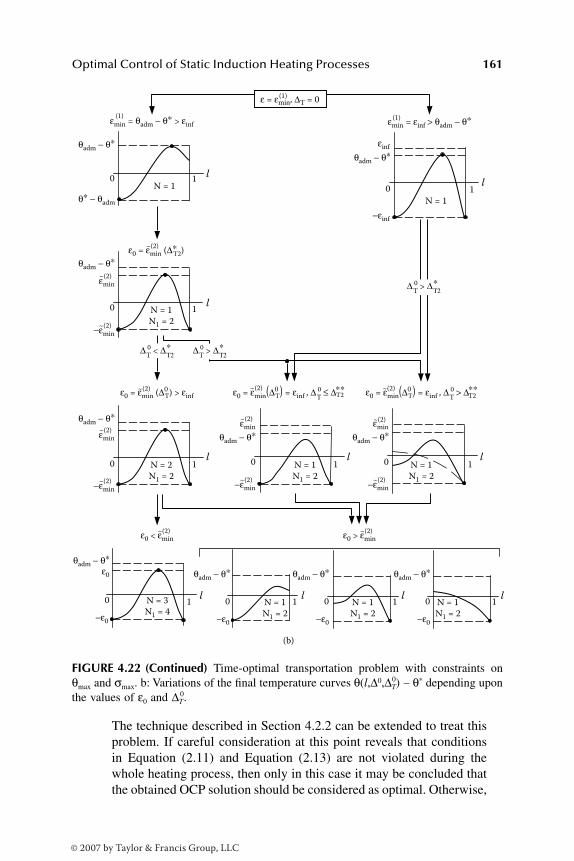
Optimal Control of Static Induction Heating Processes 161
The technique described in Section 4.2.2 can be extended to treat thisproblem. If careful consideration at this point reveals that conditionsin Equation (2.11) and Equation (2.13) are not violated during thewhole heating process, then only in this case it may be concluded thatthe obtained OCP solution should be considered as optimal. Otherwise,
FIGURE 4.22 (Continued) Time-optimal transportation problem with constraints onθmax and σmax. b: Variations of the final temperature curves θ(l,∆0,∆T)
0 – θ* depending uponthe values of ε0 and ∆T.0
(b)
εmin = θadm − θ∗ > εinf
(1)εmin = εinf > θadm − θ∗(1)
ε = εmin, ∆T = 0(1)
∆T0 > ∆∗
Τ2
∆T0 > ∆∗
Τ2∆T0 < ∆∗
Τ2
θadm − θ∗
θadm − θ∗
θadm − θ∗
θ∗ − θadm
0
0
N = 1
N = 1
N = 1
N1 = 2
N = 2
N1 = 2
N = 1
N1 = 2
N = 1
N1 = 2
N = 1
N1 = 2
N = 1
N1 = 2
N = 3
N1 = 4
1l
1l
1l
1l
1l
1l
1l
1l
ε0 = εmin (∆∗T2)
~(2)
ε0 < εmin~(2) ε0 > εmin
~(2)
ε0 = εmin (∆0T) > εinf
~(2)
εmin~(2)
εmin~(2)
−εmin~(2)
0
−εmin~(2)
θadm − θ∗εmin~(2)
0
−εmin~(2)
N = 1
N1 = 2
1l
θadm − θ∗εmin~(2)
0
−εmin~(2)
θadm − θ∗ε0
−ε0
0
θadm − θ∗
−ε0
0
θadm − θ∗
−ε0
0
θadm − θ∗
−ε0
0
θadm − θ∗
0 1l
εinf
−εinf
ε0 = εmin(∆0T) = εinf , ∆T
0 ≤ ∆∗∗~(2)T2 ε0 = εmin(∆0
T) = εinf , ∆T0 > ∆∗∗~(2)
T2
DK6039_C004.fm Page 161 Thursday, June 8, 2006 12:34 PM
© 2007 by Taylor & Francis Group, LLC
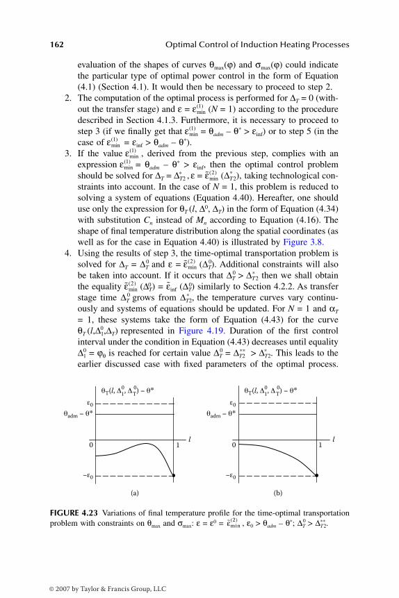
162 Optimal Control of Induction Heating Processes
evaluation of the shapes of curves θmax(ϕ) and σmax(ϕ) could indicatethe particular type of optimal power control in the form of Equation(4.1) (Section 4.1). It would then be necessary to proceed to step 2.
2. The computation of the optimal process is performed for ∆T = 0 (with-out the transfer stage) and ε = (N = 1) according to the proceduredescribed in Section 4.1.3. Furthermore, it is necessary to proceed tostep 3 (if we finally get that = θadm – θ* > εinf) or to step 5 (in thecase of = εinf > θadm – θ*).
3. If the value , derived from the previous step, complies with anexpression = θadm – θ* > εinf, then the optimal control problemshould be solved for ∆T = ∆T2 ,* ε = (∆T2),
* taking technological con-straints into account. In the case of N = 1, this problem is reduced tosolving a system of equations (Equation 4.40). Hereafter, one shoulduse only the expression for θT (l, ∆0, ∆T) in the form of Equation (4.34)with substitution Cn instead of Mn according to Equation (4.16). Theshape of final temperature distribution along the spatial coordinates (aswell as for the case in Equation 4.40) is illustrated by Figure 3.8.
4. Using the results of step 3, the time-optimal transportation problem issolved for ∆T = ∆T
0 and ε = (∆T).0 Additional constraints will also
be taken into account. If it occurs that ∆T0 > *∆T2 then we shall obtain
the equality (∆T)0 = εinf (∆T)0 similarly to Section 4.2.2. As transferstage time ∆T
0 grows from ∆T2,* the temperature curves vary continu-ously and systems of equations should be updated. For N = 1 and αT
= 1, these systems take the form of Equation (4.43) for the curveθT (l,∆1,∆T)
0 represented in Figure 4.19. Duration of the first controlinterval under the condition in Equation (4.43) decreases until equality∆1
0 = ϕθ is reached for certain value ∆T0 = ∆T2
** > ∆T2.* This leads to theearlier discussed case with fixed parameters of the optimal process.
FIGURE 4.23 Variations of final temperature profile for the time-optimal transportationproblem with constraints on θmax and σmax: ε = ε0 = , ε0 > θadm – θ*; ∆T
0 > ∆T2.**
εmin( )1
εmin( )1
εmin( )1
εmin( )1
εmin( )1
εmin( )2
εmin( )2
εmin( )2
0 1 1
(a) (b)
l l
θT(l, Δ10, Δ
T0) − θ∗ θT(l, Δ
10, Δ
T0) − θ∗
θadm − θ∗
−ε0
ε0
0
θadm − θ∗
−ε0
ε0
εmin2( )
DK6039_C004.fm Page 162 Thursday, June 8, 2006 12:34 PM
© 2007 by Taylor & Francis Group, LLC

Optimal Control of Static Induction Heating Processes 163
Then, the system of equations (Equation 4.43) for ∆10 = ϕθ takes the
following form:
(4.44)
This set can be solved with respect to unknown values ∆T2** and
(∆T2)** = (∆T2).** For all ∆T
0 > ∆T2,** the equalities N = 1, αT = 1, and ϕθ = ∆10 hold true
as before and optimal control proves to be known a priori. In this case,the maximum deviation of the final temperature from the required oneis equal to – (∆T)
0 and it is reached at the unique point l = 1 for theshape of curve 0θT(l,∆1,∆T)
0 shown in Figure 4.23a or Figure 4.23b. Thevalue of minimax (∆T)
0 = (∆T)0 can be computed directly from
the second equation in Equation (4.43).As ∆T
0 increases from ∆T2,* first, (∆T)0 < θadm – θ* and, second, the
sign of this inequality is changed to the inverse one. Therefore, depend-ing on the relationship between ∆T
0 and ∆T2,** the problem for ∆T =0∆T
and ε = (∆T)0 is reduced now to solution of the equations system
(Equation 4.43) under ∆T0 < ∆T2.** If ∆T
0 > **∆T2, then the second equationin Equation (4.43) should be solved for ∆1
0 = ϕθ.5. If the value derived from step 2 satisfies the expression = εinf
> θadm – θ* at ∆T = 0, then for any ∆T > 0 the following expression(∆T) = (∆T) > θadm – θ* would be valid. In the case of values
ε = (∆T)0 the optimal heating process is completed within one stage(N = 1) under u*(ϕ) ≡ Umax at αT = 1. In this case, the “transportation”problem is solved again for ∆T = ∆T2
** and ε = (∆T2)** under tech-nological constraints. Solution of the equations set (Equation 4.44) canbe found similarly to one described at step 4. If ∆T
0 = ∆T2,** ε0 =(∆T2),** then the initial problem proves to be solved at this stage. Under∆T
0 < ∆T2** or ∆T
0 > ∆T2,** the computational procedure is continued forε = (∆T)0 according to the technique described in step 4 (the caseof ∆T
0 > ∆T2).** In a similar manner, the alternance method can be generalized to allother possible cases. Computational sets are updated according to arequired heating accuracy ε0, transfer time ∆T,
0 and admissible temper-ature θadm. Figure 4.22b shows the variations of temperature curvesθT(l,∆0,∆T)
0 depending upon the values of ε0 and ∆T.0
4.2.4 EXAMPLES
Figure 4.24 and Figure 4.25 illustrate some computational results of time-optimalheating processes, taking into consideration the transfer stage without technological
θ ϕ θ ε
θ ϕ
θ
θ
T T
T T
0
1
22
2
, , ;
, ,
** *min
**
∆
∆
( ) − = −
( ) −
( )
θθ ε*min .= −
( ) 2
εmin( )2 εinf
εmin( )2
εmin( )2 εinf
εmin( )2
εmin( )2
εmin( )1 εmin
( )1
εmin( )2 εinf
εmin( )2
εmin( )2
εmin( )2
εmin( )2
DK6039_C004.fm Page 163 Thursday, June 8, 2006 12:34 PM
© 2007 by Taylor & Francis Group, LLC
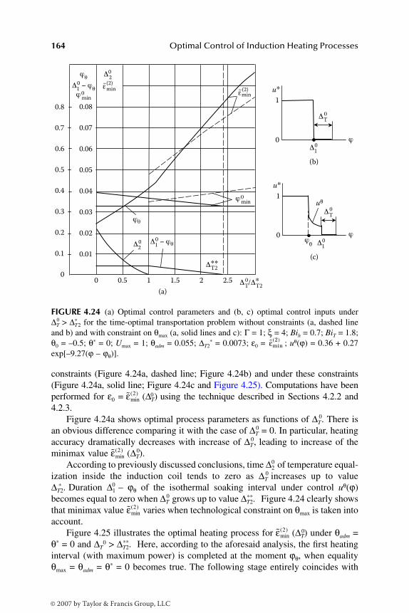
164 Optimal Control of Induction Heating Processes
constraints (Figure 4.24a, dashed line; Figure 4.24b) and under these constraints(Figure 4.24a, solid line; Figure 4.24c and Figure 4.25). Computations have beenperformed for ε0 = (∆T)0 using the technique described in Sections 4.2.2 and4.2.3.
Figure 4.24a shows optimal process parameters as functions of ∆T.0 There isan obvious difference comparing it with the case of ∆T
0 = 0. In particular, heatingaccuracy dramatically decreases with increase of ∆T,0 leading to increase of theminimax value (∆T).
0 According to previously discussed conclusions, time ∆2
0 of temperature equal-ization inside the induction coil tends to zero as ∆T
0 increases up to value∆T2.* Duration ∆1
0 – ϕθ of the isothermal soaking interval under control uθ(ϕ)becomes equal to zero when ∆T
0 grows up to value ∆T2.** Figure 4.24 clearly showsthat minimax value varies when technological constraint on θmax is taken intoaccount.
Figure 4.25 illustrates the optimal heating process for (∆T)0 under θadm =θ* = 0 and ∆T
0 > ∆T2.** Here, according to the aforesaid analysis, the first heatinginterval (with maximum power) is completed at the moment ϕθ, when equalityθmax = θadm = θ* = 0 becomes true. The following stage entirely coincides with
FIGURE 4.24 (a) Optimal control parameters and (b, c) optimal control inputs under∆T
0 > *∆T2 for the time-optimal transportation problem without constraints (a, dashed lineand b) and with constraint on θmax (a, solid lines and c): Γ = 1; ξ = 4; Bih = 0.7; BiT = 1.8;θ0 = –0.5; θ* = 0; Umax = 1; θadm = 0.055; ∆T2
* = 0.0073; ε0 = ; uθ(ϕ) = 0.36 + 0.27exp[–9.27(ϕ – ϕθ)].
0
1
0.01
0.02
0.03
0.04
0.05
0.06
0.07
0.08
min
Δ02
ε~(2)
0 0 0.5 1 1.5 2 2.5
0.1
0.2
0.3
0.4
0.5
0.6
0.7
0.8
ϕθ
Δ10 − ϕθϕ0
min
Δ20
0
1
u∗
u∗
uθ
(a)
(b)
(c)
Δ10 − ϕθ
ΔT2∗∗
ΔT0
ΔT0
ϕ0min
ϕθ
min ε~(2)
ϕ
ϕ
Δ10
Δ10ϕ
θ
ΔT0/Δ
T2∗
εmin2( )
εmin( )2
εmin( )2
εmin( )2
εmin( )2
DK6039_C004.fm Page 164 Thursday, June 8, 2006 12:34 PM
© 2007 by Taylor & Francis Group, LLC
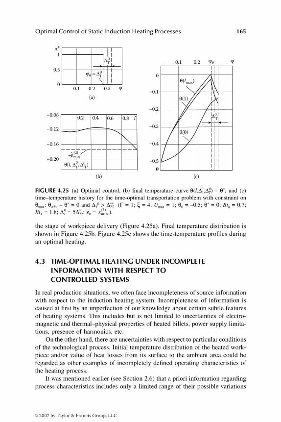
Optimal Control of Static Induction Heating Processes 165
the stage of workpiece delivery (Figure 4.25a). Final temperature distribution isshown in Figure 4.25b. Figure 4.25c shows the time-temperature profiles duringan optimal heating.
4.3 TIME-OPTIMAL HEATING UNDER INCOMPLETE INFORMATION WITH RESPECT TO CONTROLLED SYSTEMS
In real production situations, we often face incompleteness of source informationwith respect to the induction heating system. Incompleteness of information iscaused at first by an imperfection of our knowledge about certain subtle featuresof heating systems. This includes but is not limited to uncertainties of electro-magnetic and thermal–physical properties of heated billets, power supply limita-tions, presence of harmonics, etc.
On the other hand, there are uncertainties with respect to particular conditionsof the technological process. Initial temperature distribution of the heated work-piece and/or value of heat losses from its surface to the ambient area could beregarded as other examples of incompletely defined operating characteristics ofthe heating process.
It was mentioned earlier (see Section 2.6) that a priori information regardingprocess characteristics includes only a limited range of their possible variations
FIGURE 4.25 (a) Optimal control, (b) final temperature curve 0θ(l,∆1,∆T)0 – θ*, and (c)
time–temperature history for the time-optimal transportation problem with constraint onθmax: θadm – θ* = 0 and ∆T
0 > ∆T2** (Γ = 1; ξ = 4; Umax = 1; θ0 = –0.5; θ* = 0; Bih = 0.7;
BiT = 1.8; ∆T0 = 5∆T2;
* ε0 = ).
−0.080.2 0.4 0.6 0.8 l
−0.12
−0.16
−0.20
0
0.5
0.1
ϕθ = ∆10
0.2 0.3
1u∗
0
−0.1
−0.2
−0.3
−0.4
−0.5
0.1 0.2 ϕθ ϕ∆T0
(a)
(b) (c)
θ(0)
ϕ
θ
θ(1)
θ(lmax)
θ(l, ∆10, ∆0
T)
∆0T
−εmin(2)~
εmin2( )
DK6039_C004.fm Page 165 Thursday, June 8, 2006 12:34 PM
© 2007 by Taylor & Francis Group, LLC
166 Optimal Control of Induction Heating Processes
— i.e., only minimum and/or maximum values — and within these limits thesevalues could vary in an arbitrary way at each moment of time. This type ofuncertainty is often called interval uncertainty. Conditions of limited uncertaintyare quite typical for the induction heating process. In the simplest case, limiteduncertainty can be presented in the parametric form, when the appropriate char-acteristic is uniquely defined by the value of some parameter, and its value lieswithin the given range. We limit our consideration to the most typical incom-pletely determined factors that can be expressed in parametric form by theinequalities in Equation (2.20), such as the initial temperature state and value ofheat losses.
Here, the initial temperature θ0 represents the single parameter characterizinginitial temperature distribution under the assumption that it is uniform along spacecoordinates. The value of the Biot number uniquely defines heat losses from thesurface assuming heat exchange by convection at constant heat transfer coeffi-cient. Interval uncertainties of the type in Equation (2.20) could be regarded aspossible deviations (within a given range) of varied parameters from their nominalvalues, which represent constant calculated values θ0 and Bi. These deviationscould be neglected only in the case when their influence upon calculation resultsproves to be insignificant. Optimization problems considered previously havebeen solved under such assumption. However, the range of uncertainty cannot beestimated in advance. Therefore, the solution of the optimal control problemunder condition of incomplete information with respect to the heating systemcharacteristics is of vital importance.
This section shows that the proposed approach of optimal mode calculationcould be used for incompletely determined induction heating systems. To facilitateunderstanding of the proposed method, the explanations will be given with respectto the simplest IHP model and time-optimal control function.
4.3.1 PROBLEM STATEMENT
Similarly to Section 2.8, let us consider the time-optimal control problem of billetheating with given accuracy up to required temperature (the additional techno-logical constraints and transportation time will not be taken into account). Weshall assume that complete information with respect to initial temperature andheat losses is not available and that their interval uncertainty can be written inthe form of Equation (2.20). Let us suppose that each separate billet is heatedunder constant heat losses from its surface estimated by Bi number, which cantake on any invariable in time value within the range [Bimin,Bimax]. Obviously, thevalues θ0 and Bi can differ from one billet to another for different heating cycles.Keep in mind that results obtained next can be extended to other types of uncer-tainties. The technique discussed in Section 4.1 and Section 4.2 can be effectivelyapplied to the problems subject to additional constraints and the billet transferstage.
Under conditions in Equation (2.20), the problem description should berevised. Because specific values of θ0 and Bi were not defined a priori for the
DK6039_C004.fm Page 166 Thursday, June 8, 2006 12:34 PM
© 2007 by Taylor & Francis Group, LLC

Optimal Control of Static Induction Heating Processes 167
heating cycle of a particular billet, all possible values within given intervals wouldbe equally probable. Therefore, a set of controlled heating processes could beconsidered instead of one controlled system under uncertainty (Equation 2.20).Each process of this set provides the full information regarding values of θ0 andBi chosen from the range of all possible values of these uncertain factors.
In other words, each combination of fixed admissible values of θ0 and Bi (thenumber of such combinations is infinite) should be in accordance with the appro-priate heating process described by Equation (1.27) through Equation (1.31) andEquation (1.34). This means that the infinite set of such “auxiliary” heatingsystems with full information about their properties will replace real IHP underthe condition in Equation (2.20).
When governing the whole set of these objects by means of a single powercontrol, the requirement (Equation 2.25) to final temperature must be providedunder any admissible values θ0 and Bi. If we denote the final temperature distri-bution for each combination of fixed values θ0 and Bi as θ(l,θ0,Bi,ϕ0), then, insteadof Equation (2.25), the requirement to temperature distribution with given accu-racy at the end of the heating cycle can be obtained in the following form:
(4.45)
In contrast to Section 2.8, the time-optimal control problem for the heatingprocess described by Equation (1.27) through Equation (1.31) and Equation (1.34)could be formulated as follows. It is necessary to choose time-dependent powercontrol restricted by Equation (2.7) that provides steering workpiece initial tem-perature distribution to the target state (Equation 4.45) in minimal possible timeϕ0 = ϕmin.0
The optimal control algorithm, which is the solution of this problem, guar-antees that, under any possible combination of values θ0 and Bi, the requiredheating accuracy is provided at the end of the heating process. Obviously, heatingtime ϕmin,0 obtained by this algorithm, will comply with minimal possible timefor the most unfavorable combination of values θ0 and Bi. However, this timecertainly exceeds the minimal possible time for all other admissible values ofuncertain factors. Therefore, the value of the time-optimal cost function exceedsthe appropriate value attainable for the system with complete initial informationwith respect to θ0 and Bi. This cost loss is a “compensation” for guaranteedheating quality under conditions of interval uncertainty. This control algorithmimplies the guaranteed cost control approach, well known in control theory.9
It can be shown1,10 that the optimal control algorithm has the same form ofstepwise function (Equation 2.27) (Figure 2.8) as in the time-optimal problemfor the IHP model with full information about the heating system. Therefore, thetime-optimal control algorithm consists of alternating stages of heating with
max max , , , ;, ,
*
Bi ll Bi
θθ θ ϕ θ ε
0 0 10
0
∈[ ] ( ) −
≤
BBi Bi Bi∈[ ] ∈[ ]min max, , , .min maxθ θ θ0 0 0
DK6039_C004.fm Page 167 Thursday, June 8, 2006 12:34 PM
© 2007 by Taylor & Francis Group, LLC
168 Optimal Control of Induction Heating Processes
maximum power u ≡ Umax (heat ON) and subsequent soaking (heat OFF) cycles,u ≡ 0. The number of stages (N ≥ 1) is defined uniquely by given heating accuracyε. Smaller ε requires a larger number of stages N. Therefore, the profile of theoptimal control algorithm is known, but the number, N, and time durations, ∆1,∆2, …, ∆N, of the described stages remain unknown. With regard to the inequalityin Equation (4.45), the problem is reduced to the following form (similar toEquation 2.34):
(4.46)
Here, θ(l,θ0,Bi,∆) is defined as θ(l,∆) in Equation (2.34); however, in this caseθ0 and Bi represent unknown parameters meeting conditions in Equation (2.20).
4.3.2 TECHNIQUE FOR TIME-OPTIMAL PROBLEM SOLUTION UNDER INTERVAL UNCERTAINTIES
Let us introduce the vector parameter v = (l,Bi,θ0) that denotes a set of any fixedvalues:
l ∈ [0;1], Bi ∈ [Bimin; Bimax], θ0 ∈ [θ0min; θ0max].
Then, similarly to Equation (3.38), the problem (Equation 4.46) can be writtenin the following form:
(4.47)
Resemblance between the problems in Equation (3.38) and Equation (4.47)consists of the fact that, in the general statement (Equation 3.38), it is also possibleto explore the maximum of temperature deviation inside multidimensional areaΩ — i.e., within the set of spatial coordinate vectors x. At the same time, theproblem in Equation (4.47) differs from Equation (3.38) in a way that the vectorparameter v contains the parameters θ0 and Bi in addition to spatial coordinate l.
Finally, this problem becomes sufficiently complicated in comparison withEquation (2.34) due to consideration of the maximum of temperature deviationwithin the set of vector v values (instead of the set of spatial coordinate l values).
I
l
i
i
N
Bi l
∆ ∆
Φ ∆
∆( ) = →
( ) =
=
∈[ ]
∑1
0 10
min;
max max, ,θ
θ ,, , , .*θ θ ε0 Bi ∆( ) −
≤
I i
i
N
∆ ∆
Φ ∆ ∆
∆( ) = →
( ) = ( ) − ≤
=∑
1
min;
max , .*
νθ ν θ ε
DK6039_C004.fm Page 168 Thursday, June 8, 2006 12:34 PM
© 2007 by Taylor & Francis Group, LLC
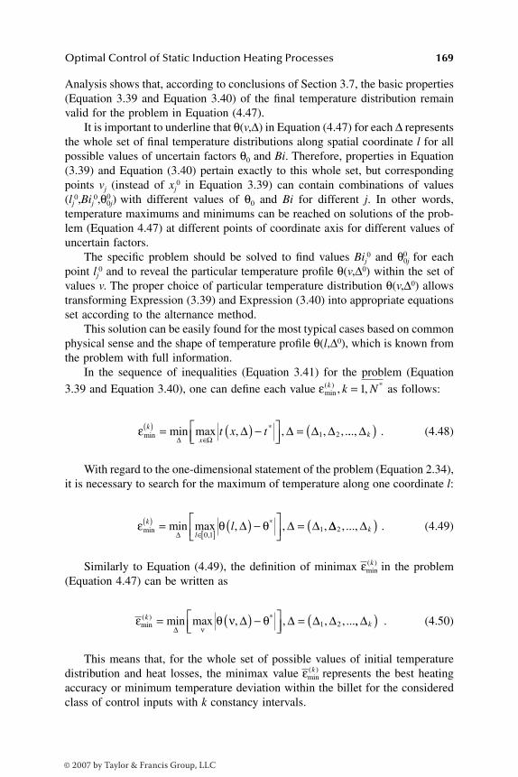
Optimal Control of Static Induction Heating Processes 169
Analysis shows that, according to conclusions of Section 3.7, the basic properties(Equation 3.39 and Equation 3.40) of the final temperature distribution remainvalid for the problem in Equation (4.47).
It is important to underline that θ(v,∆) in Equation (4.47) for each ∆ representsthe whole set of final temperature distributions along spatial coordinate l for allpossible values of uncertain factors θ0 and Bi. Therefore, properties in Equation(3.39) and Equation (3.40) pertain exactly to this whole set, but correspondingpoints vj (instead of xj
0 in Equation 3.39) can contain combinations of values(lj
0,Bij0,θ0j)
0 with different values of θ0 and Bi for different j. In other words,temperature maximums and minimums can be reached on solutions of the prob-lem (Equation 4.47) at different points of coordinate axis for different values ofuncertain factors.
The specific problem should be solved to find values Bij0 and θ0j
0 for eachpoint lj
0 and to reveal the particular temperature profile θ(v,∆0) within the set ofvalues v. The proper choice of particular temperature distribution θ(v,∆0) allowstransforming Expression (3.39) and Expression (3.40) into appropriate equationsset according to the alternance method.
This solution can be easily found for the most typical cases based on commonphysical sense and the shape of temperature profile θ(l,∆0), which is known fromthe problem with full information.
In the sequence of inequalities (Equation 3.41) for the problem (Equation
3.39 and Equation 3.40), one can define each value as follows:
. (4.48)
With regard to the one-dimensional statement of the problem (Equation 2.34),it is necessary to search for the maximum of temperature along one coordinate l:
. (4.49)
Similarly to Equation (4.49), the definition of minimax in the problem(Equation 4.47) can be written as
. (4.50)
This means that, for the whole set of possible values of initial temperaturedistribution and heat losses, the minimax value represents the best heatingaccuracy or minimum temperature deviation within the billet for the consideredclass of control inputs with k constancy intervals.
εmin( ) *, ,k k N= 1
εmin*min max , , , , .k
xt x t( )
∈= ( ) −
=
∆ Ω∆ ∆ ∆ ∆1 2 ..., ∆k( )
ε θ θmin,
*min max , , ,k
ll( )
∈[ ]= ( ) −
=∆
∆ ∆ ∆0 1
1 ∆∆ ∆2 , ..., k( )
εmin( )k
ε θ ν θν
min( ) *min max , , , , ...k = ( ) −
=
∆∆ ∆ ∆ ∆1 2 ,, ∆k( )
εmin( )k
DK6039_C004.fm Page 169 Thursday, June 8, 2006 12:34 PM
© 2007 by Taylor & Francis Group, LLC

170 Optimal Control of Induction Heating Processes
In contrast to Equation (4.49), where the values θ0 and Bi are considered asprecisely known, the search for maximum in Equation (4.50) should be imple-mented on extended argument set v = (l,Bi,θ0) rather than along the spatialcoordinate l only.
Similarly to Equation (3.1) and Equation (3.41), the following inequalitysequence holds true for values :
. (4.51)
Based on previously discussed conclusions, the following computational pro-cedure is suggested to determine optimal control algorithms for the problem(Equation 4.46).
1. At the beginning, the problem should be solved assuming that requiredheating accuracy ε in Equation (4.46) is equal to in Equation(4.51). Obviously, in this case the equality N = 1 is true, and the time-optimal heating process with accuracy consists of a single-stageheating under constant maximum power.When the surface heat losses are small enough, the temperature distri-bution θ(l,∆0) has the shape of solid curves shown in Figure 3.4 andFigure 3.6 for all possible combinations of values θ0 and Bi. In thiscase, the inequality > εinf is met, and heating accuracy could beimproved comparatively to by supplementing the process with thefurther stage of temperature soaking.According to basic properties (Equation 3.39 and Equation 3.40), forε = under N = 1, two points, v1
0 = 0(l1,Bi1,θ01)0 and0 v2
0 = 0(l2,Bi20 ,θ02
0 ) ,should be found that correspond to maximum admissible absolutedeviation of final temperature from required temperature θ*. If thetemperature profile θ(l,∆1)
0 has the shape shown in Figure 3.6, thenequalities l1
0 = 0 and l20 = le2 follow for any fixed pair of values θ0 and
Bi. The appropriate values Bi10 and θ01
0 and Bi20 and θ02
0 should be foundto reveal particular temperature profiles for which the temperatureminimum at the point l1
0 = 0 and maximum at the point l20 = le2 (Figure
4.26) are reached under the conditions in Equation (2.20). Values 0Bi1
and θ010 and Bi2
0 and θ020 respectively specify the “lower” and “upper”
temperature curves between which the possible final temperature pro-files for all other combinations of variables Bi′ and θ0′ satisfyingEquation (2.20) are situated. It is clear that temperature maximum at the point l2
0 = le2 is reachedunder maximal possible initial temperature and minimal level of heatlosses. The temperature minimum at the point l1
0 = 0, on the contrary,is reached under minimal initial temperature and maximal losses.Therefore, it follows that
εmin( )k
ε ε ε ε εmin min min min... ...1 2 1( ) ( ) ( ) +( )> > > > > >N Nmmin inf
*N( ) = ≥ε 0
εmin( )1
εmin( )1
εmin( )1
εmin( )1
εmin( )1
DK6039_C004.fm Page 170 Thursday, June 8, 2006 12:34 PM
© 2007 by Taylor & Francis Group, LLC

Optimal Control of Static Induction Heating Processes 171
. (4.52)
As a result, instead of Equation (3.12), we get the system of equations:
(4.53)
that can be solved in the same manner as Equation (3.12) with respectto ∆1, and le2.If it is necessary to provide the best heating accuracy attainableunder a single-stage control, then the initial problem is already solvedat this stage. The optimal control problem is also solved for case 1 ifthe prescribed numerical value of ε = ε0 in Equation (4.46) coincideswith the obtained numerical value of minimax . Even though ε0 <
, it is still necessary to perform step 2.
FIGURE 4.26 Variations of temperature profile for ε = at the end of time-optimalheating under incomplete information with respect to initial temperature and heat loss level.
0
Bi′, θ′0
Bi01, θ0
01
Bi02, θ0
02
1le2
l
εmin(1)−
−εmin(1)−
θ(n, ∆10) − θ∗
εmin2( )
Bi Bi Bi Bi10
010
0 20
020
0= = = =max min, ; ,min maxθ θ θ θ
θ θ θ ε
θ θ
0 0 10 1
2 0
, , , ;
,
min max*
min
max
Bi
le
∆( ) − = − ( )
,, , ;
, ,
min*
min
max min
Bi
l Bie
∆10 1
2 0
( ) − = +
∂
( )θ ε
θ θ ,,,
∆10
0( )
∂=
l
εmin( )1
εmin( )1
εmin( )1
εmin( )1
DK6039_C004.fm Page 171 Thursday, June 8, 2006 12:34 PM
© 2007 by Taylor & Francis Group, LLC

172 Optimal Control of Induction Heating Processes
2. If inequality > εinf is true, then the following computational algo-rithm is effective under condition ε0 < (see Section 3.7). Asequence of optimization problems should be solved for fixed valuesε = ε′ decreasing from by small decrement dε. Similarly to theproblem in Equation (2.34) (see Expression 3.15 and Figure 3.7), atthe beginning of this computational procedure, the value of ε′ does notappreciably deviate from value . Thus, the shape of final tempera-ture distribution and points v1
0 and v20 remains the same (even under
optimal two-stage control) as for the case of ε = (Figure 4.26).Then, instead of Equation (3.15), the following computational equa-tions set can be written:
(4.54)
In the case of fixed value ε′, this system can be solved with respect tooptimal durations ∆1
0 and ∆20 of heating/soaking intervals and
coordinate le2 of the temperature maximum. Analysis shows1 that underN = 2, the temperature distribution profile is not distorted and the setof equations (Equation 4.54) remains valid up to the value of ε′ =in Equation (4.51). According to basic properties (Equation 3.39 andEquation 3.40), for ε′ = , the third point, 0v3
0= 0(l3,Bi3,θ03),0 appears,
where maximum deviation of final temperature from the prescribedone is reached. Similarly to the problem in Equation (2.34), it ispossible to show that the expression l3
0 = 1 (see Equation 3.16 andFigure 3.8) takes place under the conditions1:
Bi30 = Bi1
0 = Bimax, θ030 = θ01
0 = θ0min.
Therefore, for ε′ = at the end of the time-optimal two-stage controlprocess, the minimal admissible temperatures are reached in the centerand on the surface of the billet if its initial temperature is minimal andthe heat loss level is maximal. At the same time, the temperaturemaximum will be located at some internal point that corresponds tothe values Bi = Bimin, θ0 = θ0max (Figure 4.27).Then, instead of Equation (3.16), the computational set of equationsfor ε′ = can be written as:
εmin( )1
εmin( )1
εmin( )1
εmin( )1
εmin( )1
θ θ θ ε
θ θ
0 0 10
20
2 0
, , , , ;
, ,
min max*
max
Bi
le
∆ ∆( ) − = − ′
BBi
l Bie
min*
max min
, , ;
, , ,
∆ ∆
∆
10
20
2 0
( ) − = + ′
∂
θ ε
θ θ 110
20
0,
.∆( )
∂=
l
εmin( )2
εmin( )2
εmin( )2
εmin( )2
DK6039_C004.fm Page 172 Thursday, June 8, 2006 12:34 PM
© 2007 by Taylor & Francis Group, LLC

Optimal Control of Static Induction Heating Processes 173
(4.55)
This set of four equations can be solved with respect to four unknowns:∆1,
0 ∆2,0 , and le2.
3. Because sets of equations are defined unambiguously depending onthe value of ε′ ∈[ ; ], for any particular value of requiredaccuracy ε = ε0 ∈[ ; ] in Equation (4.46), the computationalprocedure turns out to be quite simple.At the beginning, two problems should be solved for required accuracyvalues ε = and ε = . These problems are reduced to solutionof the equations systems (Equation 4.53 and Equation 4.55), whichallows one to find minimax values and .The optimal control problem is solved if the value of ε0 coincides withone of obtained minimaxes or . Otherwise, if the value of ε0
satisfies the condition < ε0 < , then it would still be necessaryto solve the set (Equation 4.54) for required heating accuracy. In all
FIGURE 4.27 Variations of temperature profile for ε = at the end of time-optimalheating under incomplete information with respect to initial temperature and heat losslevels.
0 1
Bi′, θ′0
Bimax, θ0 min
Bimin, θ0 max
le2
l
εmin(2)−
−εmin(2)−
θ(n, ∆0) − θ∗
εmin2( )
θ θ θ ε
θ θ
0 0 10
20 2
2
, , , , ;
,
min max*
minBi
le
∆ ∆( ) − = − ( )
00 10
20 2
01
max min*
min
min
, , , ;
, ,
Bi ∆ ∆( ) − = + ( )θ ε
θ θ BBi
l Bie
max*
min
max
, , ;
, ,
∆ ∆10
20 2
2 0
( ) − = −
∂
( )θ ε
θ θ mmin , ,.
∆ ∆10
20
0( )
∂=
l
εmin( )2
εmin( )2 εmin
( )1
εmin( )2 εmin
( )1
εmin( )1 εmin
( )2
εmin( )1 εmin
( )2
εmin( )1 εmin
( )2
εmin( )2 εmin
( )1
DK6039_C004.fm Page 173 Thursday, June 8, 2006 12:34 PM
© 2007 by Taylor & Francis Group, LLC
174 Optimal Control of Induction Heating Processes
equations, the temperature dependencies are calculated by formulas(Equation 2.28 and Equation 2.29) under appropriate values of θ0 andBi.If condition ε0 < is true, then the solution should be found usingthe computational technique for optimal processes with complete infor-mation with respect to the controlled system (Chapter 3).
Figure 4.28 shows some results of computation that are provided as anexample of the proposed method for time-optimal induction heating of an infinitecylinder under conditions in Equation (2.20).
Calculations were performed for values ε ∈[ , ]. Optimal final tem-perature distributions along the cylinder radius are shown in Figure 4.28a andFigure 4.28b for the most typical values of required heating accuracy and
. Figure 4.28c shows optimal process time as a function of ε compared toresults for the controlled system with complete information with respect to initialdata. Figure 4.28d (as well as Figure 4.28c) illustrates the total process time lossin contrast to optimal process calculated for precisely determined values of θ0
and Bi.
4.4 HEATING PROCESS WITH MINIMUM PRODUCT COST
The cost of product can be regarded as one of the IHP quality indexes in certainproduction situations (Section 2.2). When a criterion of minimum cost is required,depending upon application, all major IHI performance characteristics can beconsidered, including productivity, quality of product, power cost, and materiallosses. The overall product cost can be estimated by a combined criterion (Equa-tion 2.5) that includes all cost components (Equation 2.2 through Equation 2.4)with weighting coefficients Ci making sense of a relative costing and representingthe importance of each of the items of the overall cost.
Some aspects of the minimum cost problem in application to static inductionheating prior to hot forming of metals are discussed in this section. To makeunderstanding easier, the one-dimensional linear model of the heating processwill be used here. To simplify discussion, the technological constraints can beneglected during the first stage of the process of finding the OCP solution. Theheated billet’s transfer stage and incomplete information regarding the heatingsystem will also not be considered. It is important to keep in mind that obtainedresults can be extended onto problems subject to technological constraints andother complicating factors by using techniques described in Section 4.1 throughSection 4.3.
Heating accuracy, energy consumption, metal loss due to scale, and heatingprocess time represent main components of product cost (Section 2.2). It wasshown earlier that the alternance method has been successfully applied for opti-mization of the heating process with respect to maximum accuracy or minimum
εmin( )2
εmin( )2 εmin
( )1
εmin( )1
εmin( )2
DK6039_C004.fm Page 174 Thursday, June 8, 2006 12:34 PM
© 2007 by Taylor & Francis Group, LLC
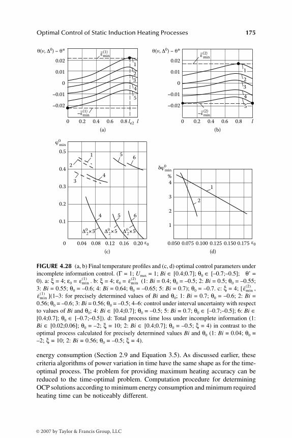
Optimal Control of Static Induction Heating Processes 175
energy consumption (Section 2.9 and Equation 3.5). As discussed earlier, thesecriteria algorithms of power variation in time have the same shape as for the time-optimal process. The problem for providing maximum heating accuracy can bereduced to the time-optimal problem. Computation procedure for determiningOCP solutions according to minimum energy consumption and minimum requiredheating time can be noticeably different.
FIGURE 4.28 (a, b) Final temperature profiles and (c, d) optimal control parameters underincomplete information control. (Γ = 1; Umax = 1; Bi ∈ [0.4;0.7]; θ0 ∈ [–0.7;–0.5]; θ* =0). a: ξ = 4; ε0 = . b: ξ = 4; ε0 = (1: Bi = 0.4; θ0 = –0.5; 2: Bi = 0.5; θ0 = –0.55;3: Bi = 0.55; θ0 = –0.6; 4: Bi = 0.64; θ0 = –0.65; 5: Bi = 0.7); θ0 = –0.7. c: ξ = 4; [ ,
](1–3: for precisely determined values of Bi and θ0; 1: Bi = 0.7; θ0 = –0.6; 2: Bi =0.56; θ0 = –0.6; 3: Bi = 0.56; θ0 = –0.5; 4–6: control under interval uncertainty with respectto values of Bi and θ0; 4: Bi ∈ [0.4;0.7]; θ0 = –0.5; 5: Bi = 0.7; θ0 ∈ [–0.7;–0.5]; 6: Bi ∈[0.4;0.7]; θ0 ∈ [–0.7;–0.5]). d: Total process time loss under incomplete information (1:Bi ∈ [0.02;0.06]; θ0 = –2; ξ = 10; 2: Bi ∈ [0.4;0.7]; θ0 = –0.5; ξ = 4) in contrast to theoptimal process calculated for precisely determined values Bi and θ0 (1: Bi = 0.04; θ0 =–2; ξ = 10; 2: Bi = 0.56; θ0 = –0.5; ξ = 4).
0.1
0
0.2
0.3
0.4
0.5
0.04 0.08 0.12 0.16 0.20
1
2
3 4
5
4
Δ02×5 Δ0
2×5 Δ02×5
5 6
6
1
2
3
4
0.050 0.075 0.100 0.125 0.150 0.175
%
1
2
0
−0.02
−0.01
0.02
0.01
0.2 0.4 0.6 0.8 le2 l 0 0.2 0.4
(b) (a)
(c) (d)
0.6 0.8 l 0
1
2
3
4
5
1
2
3
4
5
θ(v, Δ0) − θ∗
ϕ0min
δϕ0min
ε0 ε0
0
−0.02
−0.01
0.02
0.01
θ(v, Δ0) − θ∗εmin‒(1)
εmin
−εmin −εmin
‒(2)
‒(2) ‒(1)
εmin1( ) εmin
2( )
εmin2( )
εmin1( )
DK6039_C004.fm Page 175 Thursday, June 8, 2006 12:34 PM
© 2007 by Taylor & Francis Group, LLC

176 Optimal Control of Induction Heating Processes
Metal losses due to scale formation represent one of the most essentialexpense components of IHP product cost. Problems of minimum metal loss dueto scale formation differ significantly from the optimization problems studiedearlier and will be discussed later. Several approaches will be considered to defineheating modes that are optimal with respect to overall cost function (Equation2.5).
4.4.1 PROBLEM OF METAL SCALE MINIMIZATION
4.4.1.1 Overview of Optimal Heating Modes
Cost of material represents an essential part of product cost. For high-temperatureheating applications, the appreciable portion of material expenses deals with metalloss due to scale formation. As shown in Butkovskij et al.,11,12 the value of metalloss can also be considered as the optimization criterion and could be written inintegral form (Equation 2.4). The integrand in Expression (2.4) can be representedin an exponential form. Using the system of relative units (see Chapter 1), acriterion of metal scale minimization can be written as:
(4.56)
where
(4.57)
Expression (4.57) is obtained under assumption that the process of metal oxida-tion (scale formation) occurs only when the billet’s surface temperature θsur
exceeds the given value θq.Let us consider the heating process that can be described by Equation (1.27)
through Equation (1.35). The surface temperature θsur can be easily found bysubstituting l = 1 in the function θ(l,ϕ). This process calls for total consumedheating power u(ϕ) as a lumped control input. Formula (2.25) can be used fortemperature requirements at the end of the heating cycle.
The statement of the problem for minimizing metal loss due to scale can beformulated as follows. It is necessary to select such power control function u*(ϕ)bounded by restraint (Equation 2.7) that provides steering workpiece initial tem-perature distribution to the desired temperature θ* with prescribed accuracy ε(according to Equation 2.25) for the given time ϕ0 and holds the cost criterion(Equation 4.56 and Equation 4.57) at the minimal level.
I f dsur= ( )( ) →∫0
0ϕ
θ ϕ ϕ min
fif
ifsur
sur q
sur qS
sur
θ ϕθ θ
θ θ θ( )( ) =
≤
−( ) ≥+
0
1
, ;
, θθq .
DK6039_C004.fm Page 176 Thursday, June 8, 2006 12:34 PM
© 2007 by Taylor & Francis Group, LLC

Optimal Control of Static Induction Heating Processes 177
At the beginning, it is necessary to define the shape of optimal control functionu*(ϕ). In this case, the optimal power control does not consist of alternating stagesof heating with maximum power u ≡ Umax (heat ON) and subsequent soaking/cool-ing under u ≡ 0 (heat OFF) cycles. Therefore, control will look quite differentcompared to solutions of OCP for minimum time, maximum heating accuracy,and minimum energy consumption criteria.
If desired final temperature θ* exceeds θq (usually θsur ≅ 600 to 650°), thenthe minimal amount of scale is obtained for the fixed time ϕ0, if the billet’s surfacetemperature will vary in time, in the following way. On the one hand, the surfacetemperature at any moment ϕ0 (see Equation 4.56 and Equation 4.57) must beas close to the value of θq as possible. On the other hand, to achieve the requiredtemperature distribution that satisfies the condition θ* > θq, the expression θsur >θq should be valid during a certain stage of the process. It is clear that acceleratedheating mode under u(ϕ) ≡ Umax does not meet this purpose because it results inmaximum temperature gradients (under maximum values of θsur) and, therefore,leads to a greater amount of metal loss due to scale.
It is possible to show11,12 that if the required final temperature θ* exceedstemperature θq of intensive oxidation, then metal losses become minimum underexponential variation of θsur over time:
θsur(ϕ) = AeBϕ + θq , (4.58)
where A, B > 0 are positive coefficients.Let us notice that the optimal surface temperature already exceeds θq at initial
moment ϕ = 0. Optimal power control u*(ϕ), which provides variation of billetsurface temperature according to Expression (4.58), can be found based on thegeneral expression (Equation 1.36) for temperature distribution. If function θsur(ϕ)is given in the form of Equation (4.58) then Equation (1.36) at l = 1 could beconsidered as the integral equation with respect to control function u* (ϕ). Itssolution can be found in the same way as in the case of the functions uσ(ϕ) anduθ(ϕ) (Section 4.1).
However, it turns out that, as a rule, realization of the algorithm in Equation(4.58) by means of admissible controls over the whole duration of the heatingprocess is impossible. This conclusion is stipulated by a number of certainpractical conditions.
In reality, the initial surface temperature is less than the oxidation thresholdθq. Obviously, it is impossible to raise the value of θsur momentarily up to thevalue θsur(0) > θq under limited heating power Umax in Expression (2.7) as isrequired in Equation (4.58). Thus, the initial stage of the optimal process can beconducted under maximum power u*(ϕ) ≡ Umax that leads to the maximal possiblerise of surface temperature up to the values, which are required according to thealgorithm (Equation 4.58).
Optimal heating mode depends to a greater extent upon given duration ϕ0 ofthe heating process. Expression (4.58) remains valid if sufficient slack time existsbecause it provides minimal possible excess of θsur over θq. If there is no extratime, then it is impossible to apply this algorithm during the whole process.
DK6039_C004.fm Page 177 Thursday, June 8, 2006 12:34 PM
© 2007 by Taylor & Francis Group, LLC
178 Optimal Control of Induction Heating Processes
As an example, let us consider the case of value ϕ0 that is equal to minimumtime ϕmin
0 required for heating with the same accuracy ε up to the same finaltemperature θ* in Equation (2.25). As shown earlier, the optimal control algorithmu*(ϕ) in this case could be represented by only the time-dependent stepwisefunction in the form of Equation (2.27). Such control does not allow reducingthe scale. This means that for ϕ0 = 0ϕmin the value of the criterion (Equation (4.56)should be considered as optimal under control function Equation (2.27)).
If the condition ϕ0 > ϕmin0 is met, then the optimal process includes separate
stages of heating according to the algorithm (Equation 4.58). The optimal algo-rithm comprises stages of heating with maximum power u*(ϕ) ≡ Umax and sub-sequent soaking under u*(ϕ) ≡ 0 that conform to time-optimal control.
Therefore, one can conclude that the sought optimal algorithm consists ofstages of heating with maximum power u ≡ Umax and subsequent soaking/coolingunder u ≡ 0, as well as different intervals, that provide the exponential law ofsurface temperature growth. The latter intervals can be called singular intervalsand appropriate control functions us(ϕ) can be called singular control functions.13
In the general case, the number of control stages and their sequence depend upongiven accuracy ε in Equation (2.25) and cannot be easily defined. Calculation ofsingular control functions adds additional complexity to this problem comparedto the conventional one. An approximate solution of such a problem is considerednext for the most typical values of required heating accuracy.
4.4.1.2 Two-Parameter Power Control Algorithm of Scale Minimization
Let us consider the case of ϕ0 = ϕmin0 in Equation (4.56) that allows one to
transform the problem of minimum scale into the time-optimal problem (Equation2.34). Let us assume that ε = . Figure 3.8 shows the shape of the time-optimalcontrol algorithm that can be defined by two parameters: durations ∆1
0 and ∆20 of
heating and soaking intervals. Parameters ∆10 and ∆2
0 can be found after solvingthe set of equations in Equation (3.16). Figure 3.8a (curve 2) shows the appro-priate spatial temperature distribution at the end of the optimal process. Fortemperature profile of that shape, there will be three points within the heatedworkpiece (l = 0, l = le2, and l = 1) where maximum admissible deviations of thefinal temperature from the required one exist.
Let us assume that the given heating time exceeds the time ϕmin0 ( ) by the
relatively small value of dϕ0 > 0. We shall consider the problem of minimumscale under ϕ0 = 0ϕmin( ) + dϕ0 for a certain attainable value ε in Equation(2.25) that differs from by value dε of order dϕ0.
The continuous nature of all optimal process parameters as functions of ϕ0
and ε allows one to conclude that small variations of dϕ0 and dε lead to smallvariations in the optimal control algorithm and the final temperature distributionprofile. This means that there will be a maximum of three points within the heatedworkpiece where maximum admissible deviations of the final temperature fromthe required one exist. In contrast to the time-optimal problem, the minimum
εmin( )2
εmin( )2
εmin( )2
εmin( )2
DK6039_C004.fm Page 178 Thursday, June 8, 2006 12:34 PM
© 2007 by Taylor & Francis Group, LLC
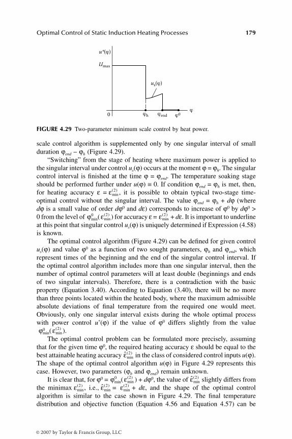
Optimal Control of Static Induction Heating Processes 179
scale control algorithm is supplemented only by one singular interval of smallduration ϕend – ϕh (Figure 4.29).
“Switching” from the stage of heating where maximum power is applied tothe singular interval under control us(ϕ) occurs at the moment ϕ = ϕh. The singularcontrol interval is finished at the time ϕ = ϕend. The temperature soaking stageshould be performed further under u(ϕ) ≡ 0. If condition ϕend = ϕh is met, then,for heating accuracy ε = , it is possible to obtain typical two-stage time-optimal control without the singular interval. The value ϕend = ϕh + dϕ (wheredϕ is a small value of order dϕ0 and dε) corresponds to increase of ϕ0 by dϕ0 >0 from the level of 0ϕmin( ) for accuracy ε = + dε. It is important to underlineat this point that singular control us(ϕ) is uniquely determined if Expression (4.58)is known.
The optimal control algorithm (Figure 4.29) can be defined for given controlus(ϕ) and value ϕ0 as a function of two sought parameters, ϕh and ϕend, whichrepresent times of the beginning and the end of the singular control interval. Ifthe optimal control algorithm includes more than one singular interval, then thenumber of optimal control parameters will at least double (beginnings and endsof two singular intervals). Therefore, there is a contradiction with the basicproperty (Equation 3.40). According to Equation (3.40), there will be no morethan three points located within the heated body, where the maximum admissibleabsolute deviations of final temperature from the required one would meet.Obviously, only one singular interval exists during the whole optimal processwith power control u*(ϕ) if the value of ϕ0 differs slightly from the value
0ϕmin( ).The optimal control problem can be formulated more precisely, assuming
that for the given time ϕ0, the required heating accuracy ε should be equal to thebest attainable heating accuracy in the class of considered control inputs u(ϕ).The shape of the optimal control algorithm u(ϕ) in Figure 4.29 represents thiscase. However, two parameters (ϕh and ϕend) remain unknown.
It is clear that, for ϕ0 = 0ϕmin( ) + dϕ0, the value of slightly differs fromthe minimax , i.e., = + dε, and the shape of the optimal controlalgorithm is similar to the case shown in Figure 4.29. The final temperaturedistribution and objective function (Equation 4.56 and Equation 4.57) can be
FIGURE 4.29 Two-parameter minimum scale control by heat power.
0
Umax
u*(ϕ)
us(ϕ)
ϕh ϕend ϕ0ϕ
εmin( )2
εmin( )2 εmin
( )2
εmin( )2
ˆmin( )ε 2
εmin( )2 ˆ
min( )ε 2
εmin( )2 ˆ
min( )ε 2 εmin
( )2
DK6039_C004.fm Page 179 Thursday, June 8, 2006 12:34 PM
© 2007 by Taylor & Francis Group, LLC
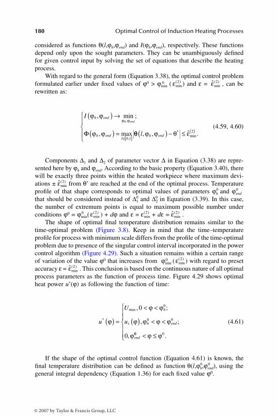
180 Optimal Control of Induction Heating Processes
considered as functions θ(l,ϕh,ϕend) and I(ϕh,ϕend), respectively. These functionsdepend only upon the sought parameters. They can be unambiguously definedfor given control input by solving the set of equations that describe the heatingprocess.
With regard to the general form (Equation 3.38), the optimal control problemformulated earlier under fixed values of ϕ0 > ϕmin
0 ( ) and ε = , can berewritten as:
(4.59, 4.60)
Components ∆1 and ∆2 of parameter vector ∆ in Equation (3.38) are repre-sented here by ϕh and ϕend. According to the basic property (Equation 3.40), therewill be exactly three points within the heated workpiece where maximum devi-ations ± from θ* are reached at the end of the optimal process. Temperatureprofile of that shape corresponds to optimal values of parameters ϕh
0 and ϕend0
that should be considered instead of ∆10 and ∆2
0 in Equation (3.39). In this case,the number of extremum points is equal to maximum possible number underconditions ϕ0 = 0ϕmin( ) + dϕ and ε = + dε = .
The shape of optimal final temperature distribution remains similar to thetime-optimal problem (Figure 3.8). Keep in mind that the time–temperatureprofile for process with minimum scale differs from the profile of the time-optimalproblem due to presence of the singular control interval incorporated in the powercontrol algorithm (Figure 4.29). Such a situation remains within a certain rangeof variation of the value ϕ0 that increases from 0ϕmin
( ) with regard to presetaccuracy ε = . This conclusion is based on the continuous nature of all optimalprocess parameters as the function of process time. Figure 4.29 shows optimalheat power u*(ϕ) as following the function of time:
(4.61)
If the shape of the optimal control function (Equation 4.61) is known, thefinal temperature distribution can be defined as function 0θ(l,ϕh,ϕend),
0 using thegeneral integral dependency (Equation 1.36) for each fixed value ϕ0.
εmin( )2 ˆ
min( )ε 2
I h end
h endl
h end
ϕ ϕ
ϕ ϕ
ϕ ϕ, min ;
, max
,
,
( ) →
( ) =∈[ ]
Φ0 1
θθ ϕ ϕ θ εl h end, , ˆ .*min( ) − ≤
( )2
ˆmin( )ε 2
εmin( )2 εmin
( )2 ˆmin( )ε 2
εmin( )2
ˆmin( )ε 2
u
U
u
h
s h end
end
*
max , ;
, ;
,
ϕ
ϕ ϕ
ϕ ϕ ϕ ϕ
ϕ
( ) =< <
( ) < <
0
0
0
0 0
00 0< ≤
ϕ ϕ .
DK6039_C004.fm Page 180 Thursday, June 8, 2006 12:34 PM
© 2007 by Taylor & Francis Group, LLC

Optimal Control of Static Induction Heating Processes 181
If the final temperature profile replicates the curve in Figure 3.8, then, accord-ing to basic properties (Equation 3.39 and Equation 3.40) and similar to Equation(3.16), the computational set of equations should be considered in the followingform with respect to ϕh
0 and ϕend:0
(4.62)
This system differs from Equation (3.16) by expression θ(l,ϕh,ϕend) with respectto a final temperature distribution in comparison with 0θ(l,∆1,∆2).
0 Similarly to Equa-tion (3.16), the set in Equation (4.62) can be solved with respect to four unknownvariables: optimal values ϕh
0 and ϕend0 of the beginning and the end of the singular
control interval; minimax ; and an intermediate unknown variable — coordi-nate le2 of the point of temperature maximum.
The optimal power control algorithm in the form of Equation (4.61) can befound only under a priori known singular control us(ϕ) during the interval[ϕh;ϕend]. It is possible to show that if two terms of the infinite series are used inexpression for temperature field, then singular control can be found as a solutionof the appropriate integral equation. In the conventional case of uniform initialtemperature distribution θ0(l) ≡ θ0 = θa = const, the singular control function canbe obtained under the boundary condition (Equation 1.34) in Equation (1.27)through Equation (1.35) as follows1,14:
. (4.63)
Constant coefficients C1, C2, C3, and A1, A2 should be calculated accordingto the following formulas:
θ ϕ ϕ θ ε
θ ϕ ϕ
0 0 0 2
20 0
, , ˆ ;
, ,
*minh end
e h endl
( ) − = −
(
( )
)) − = +
( ) − = −
( )
( )
θ ε
θ ϕ ϕ θ ε
*min
*min
ˆ ;
, , ˆ
2
0 0 21 h end ;;
, ,.
∂ ( )∂
=
θ ϕ ϕl
l
e h end20 0
0
ˆmin( )ε 2
u C e C e Cs
A
s Ah end
hhϕ ϕ ϕ ϕ
ϕ ϕ ϕ ϕ( ) = + + ∈−( ) −( )
1 2 3
12 , ,[[ ]
DK6039_C004.fm Page 181 Thursday, June 8, 2006 12:34 PM
© 2007 by Taylor & Francis Group, LLC
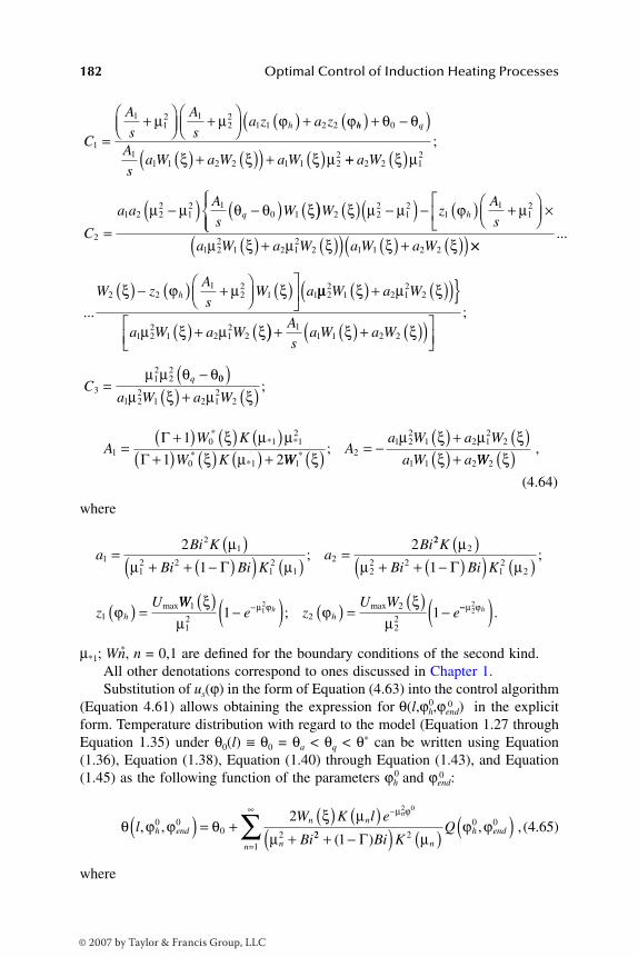
182 Optimal Control of Induction Heating Processes
,
(4.64)
where
µ*1; Wn,* n = 0,1 are defined for the boundary conditions of the second kind.All other denotations correspond to ones discussed in Chapter 1. Substitution of us(ϕ) in the form of Equation (4.63) into the control algorithm
(Equation 4.61) allows obtaining the expression for 0θ(l,ϕh,ϕend)0 in the explicitform. Temperature distribution with regard to the model (Equation 1.27 throughEquation 1.35) under θ0(l) ≡ θ0 = θa < θq < θ* can be written using Equation(1.36), Equation (1.38), Equation (1.40) through Equation (1.43), and Equation(1.45) as the following function of the parameters ϕh
0 and ϕend:0
, (4.65)
where
C
A
s
A
sa z a zh
1
112 1
22
1 1 2 2
=+
+
( ) +µ µ ϕ ϕhh q
A
sa W a W a W
( ) + −( )( ) + ( )( ) + ( )
θ θ
ξ ξ ξ µ
0
11 1 2 2 1 1 2
2 ++ ( )
=−( ) −( ) (
a W
C
a aA
sWq
2 2 12
2
1 2 22
12 1
0 1
ξ µ
µ µ θ θ ξ
;
)) ( ) −( ) − ( ) +
×
W zA
sh2 2
212
11
12ξ µ µ ϕ µ
( ) + ( )( ) ( ) + ( )( )a W a W a W a W1 2
21 2 1
22 1 1 2 2µ ξ µ ξ ξ ξ ××
( ) − ( ) +
( )
...
...
W zA
sW ah2 2
122
1 1ξ ϕ µ ξ µµ ξ µ ξ
µ ξ µ ξ
22
1 2 12
2
1 22
1 2 12
2
W a W
a W a W
( ) + ( )( )( ) + ( )) + ( ) + ( )( )
=−
A
sa W a W
Cq
11 1 2 2
312
22
ξ ξ
µ µ θ θ
;
00
1 22
1 2 12
2
( )( ) + ( )a W a Wµ ξ µ ξ
;
AW K
W K1
0 1 12
0 1
1
1 2=
+( ) ( ) ( )+( ) ( ) ( ) +Γ
Γ
** *
**
ξ µ µξ µ WW
Aa W a W
a W a12
1 22
1 2 12
2
1 1 2* ;
ξµ ξ µ ξ
ξ( ) = −( ) + ( )( ) + WW2 ξ( )
aBi K
Bi Bi Ka
Bi1
21
12 2
12
12
2
1
2= ( )
+ + −( )( ) ( )=
µµ µΓ
;22
2
22 2
12
2
1
1
K
Bi Bi K
zU
h
µµ µ
ϕ
( )+ + −( )( ) ( )
( ) =
Γ;
maxWWe z
U Weh
h1
12 2
2
221 11
2ξµ
ϕξ
µµ ϕ( )
−( ) ( ) = ( )−− ;
max −−( )µ ϕ22
h .
θ ϕ ϕ θξ µ
µ
µ ϕ
lW K l e
Bih end
n n
n
n
, ,0 00 2
22 0
( ) = +( ) ( )
+
−
22 20 0
11+ −( ) ( ) ( )
=
∞
∑ ( ),
Γ Bi KQ
n
h end
nµ
ϕ ϕ
DK6039_C004.fm Page 182 Thursday, June 8, 2006 12:34 PM
© 2007 by Taylor & Francis Group, LLC

Optimal Control of Static Induction Heating Processes 183
(4.66)
Expression (4.66) should be used to solve the set of equations in Equation (4.62).It is important to underline that the optimal algorithm (Equation 4.61) is
found approximately using a singular control in the form of Equation (4.63) andtaking into account only two terms of the Fourier series that describes temperaturefield within the billet. However, the final temperature distribution is preciselydefined based on the mathematical model in the form of an infinite series in(Equation 4.65). A sufficiently large number of series terms in Equation (4.65)must be considered for calculating the temperature distribution with satisfactoryaccuracy. Therefore, exact OCP solution provides the desired final temperaturedistribution under the control input that can be considered only as approximatelyoptimal with respect to the criterion of scale minimization.
Let us consider as an example the optimal control mode when it is necessaryto provide the best heating accuracy ε = . Figure 4.30 shows the results of
FIGURE 4.30 a: Optimal control and time–temperature history; b: radial temperatureprofile θ(l,ϕh
0,ϕend)0 – θ* at the end of minimum scale heating. Γ = 1; ξ = 4; Umax = 1 θ0
= –0.5; θ* = 0; θq = –0.125; S = 3.5; ε0 = ; ϕ0 = 0.44 > ϕend.0
Q U eC e
A
s
h end
A
sn h
h
ϕ ϕ
µ
µ ϕϕ
0 0 1
1
2 0
1 0
1, max( ) = −( ) +−
nn
A
s
A
se en end n h
2 1
1 2 0 1 2 0
+−
+
+
µ ϕ µ ϕ
+
++
−−
+( )C eA
e eA
n
A Ahn end2
22
20
22 0
1
ϕµ ϕ
µ
222 0 2 0 2 0
3+( )
+ −( )µ ϕ µ ϕ µ ϕn h n end n hC e e .
ˆmin( )ε 2
0.1 0.2 0.3 ϕ 0
0.5
(a)
(b)
1
u∗
u∗
−0.1
−0.2
−0.3
−0.4
θq θ(0)
θ − θ∗
ϕh0 ϕ0 ϕ0
end
θ(1)
0
0.01
−0.01
10.4 0.8
l le2
–εmin(2)^
εmin2( )
DK6039_C004.fm Page 183 Thursday, June 8, 2006 12:34 PM
© 2007 by Taylor & Francis Group, LLC

184 Optimal Control of Induction Heating Processes
the optimal problem for minimizing metal loss due to scale formation. Compu-tations have been performed according to the previously described technique.Expressions for final optimal control u*(ϕ) and temperature distributionθ(l,ϕh,ϕend)
0 in0 the form of Equation (4.61), Equation (4.63), and Equation (4.65)were used in all sets of equations. Figure 4.30a shows optimal control andtime–temperature profiles for the billet surface (l = 1) and its center during theheating process. Figure 4.30b represents radial temperature distribution that takesplace at the end of the optimal heating cycle.
A sequence of optimization problems should be solved for fixed values ϕ0,increasing from 0ϕmin( ) by a relatively small step. Study of obtained resultscould reveal a sensitivity of optimal control algorithms as a function of valuesof ϕ0 with regard to basic properties (Equation 3.39 and Equation 3.40). Com-putational results for initial data in Figure 4.30 allow one to conclude that theshape of the final temperature curve and, therefore, sets of computational equa-tions, the optimal control algorithm, and expression for final temperature distri-bution remain unchanged in spite of the increase of given value ϕ0. At the sametime, duration of soaking interval under u*(ϕ) ≡ 0 reduces monotonously, and thedifference ϕ0 – ϕend
0 tends to zero (Figure 4.29). The equality ϕ10 = ϕend
0 becomesvalid under the certain value ϕ0 = ϕ1,
0 and the optimal heating process comes tothe end during the singular control interval (Figure 4.31).
In this case, one should accept ϕ0 = ϕ10 = ϕend
0 in Expression (4.65) andExpression (4.66) for temperature distribution 0θ(l,ϕh,ϕend).0 The value of ϕ0, whichin this case is equal to ϕ1,
0 can be found by solving the set of equations in Equation(4.62) with respect to ϕh
0 and ϕend0 = ϕ1.
0 Figure 4.32 shows some results ofcomputation for ϕ0 = ϕ1.
0 As can be seen in Figure 4.32b, the shape of curveθ(l,ϕh
0 ,ϕend)0 remains unchanged if the condition ϕ0 = ϕ10 is not violated. Based
on the continuous nature of dependency θ(l,ϕh0 ,ϕend)0 on ϕ0, it is possible to
conclude that the final temperature profile remains the same even though therewas an increase of the time ϕ0 by a small value (in comparison with 0ϕ1).
Similarly to the previous discussion, the optimal control algorithm for cor-responding values of ϕ0 should include only one singular interval. At the same
FIGURE 4.31 Two-parameter minimum scale control by heat power when the optimalheating process comes to the end during the singular control interval.
0
ϕh0 ϕ
10 = ϕ0
end
ϕ
u∗(ϕ)
Umax
εmin( )2
DK6039_C004.fm Page 184 Thursday, June 8, 2006 12:34 PM
© 2007 by Taylor & Francis Group, LLC
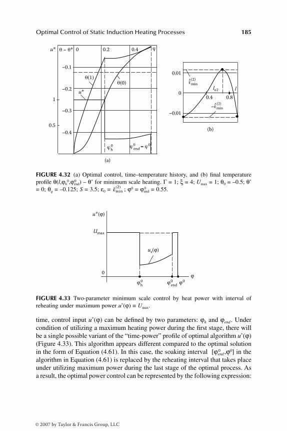
Optimal Control of Static Induction Heating Processes 185
time, control input u*(ϕ) can be defined by two parameters: ϕh and ϕend . Undercondition of utilizing a maximum heating power during the first stage, there willbe a single possible variant of the “time-power” profile of optimal algorithm u*(ϕ)(Figure 4.33). This algorithm appears different compared to the optimal solutionin the form of Equation (4.61). In this case, the soaking interval 0[ϕend ,ϕ0] in thealgorithm in Equation (4.61) is replaced by the reheating interval that takes placeunder utilizing maximum power during the last stage of the optimal process. Asa result, the optimal power control can be represented by the following expression:
FIGURE 4.32 (a) Optimal control, time–temperature history, and (b) final temperatureprofile θ(l,ϕh
0,ϕend)0 – θ* for minimum scale heating. Γ = 1; ξ = 4; Umax = 1; θ0 = –0.5; θ*
= 0; θq = –0.125; S = 3.5; ε0 = ; ϕ0 = ϕend0 = 0.55.
FIGURE 4.33 Two-parameter minimum scale control by heat power with interval ofreheating under maximum power u*(ϕ) ≡ Umax.
0
0.5
1
0.2 0.4 ϕθ − θ∗
(a)
(b)
u∗
u∗
−0.1
−0.2
−0.3
−0.4
θ(0)
ϕh0 ϕ0
end = ϕ0
θ(1)
0
0.01
−0.01
0.4 0.8
l le2
εmin∧(2)
−εmin∧(2)
εmin2( )
0
ϕh0 ϕ0ϕ0
end
ϕ
us(ϕ)
u∗(ϕ)
Umax
DK6039_C004.fm Page 185 Thursday, June 8, 2006 12:34 PM
© 2007 by Taylor & Francis Group, LLC

186 Optimal Control of Induction Heating Processes
(4.67)
The singular control us(ϕ) can be defined according to Equation (4.63) andEquation (4.64), and computational equation set (Equation 4.62) remainsunchanged. However, the expression for θ(l,ϕh
0,ϕend)0 is obtained similarly toEquation (4.65) and Equation (4.66), and it should be modified according tovariation of optimal algorithm u*(ϕ).
Computation results show that the shapes of radial temperature distributionθ(l,ϕh
0 ,ϕend)0 – θ* (compare with Figure 4.32b), the control algorithm (Equation4.67), and the set of equations (Equation 4.62) remain unchanged when presetheating time ϕ0 increases beyond all bounds from the value of ϕ1.
0 The minimalvalue of cost function I(ϕh
0,ϕend)0 in Equation (4.59) asymptotically decreaseswith increase of the time ϕ0. The time ϕh
0 required for heating under maximumpower also decreases to limiting value
when billet surface temperature becomes equal to oxidation threshold:
θsur(ϕhmin)0 = θq.
Some results of computation in Figure 4.34a through Figure 4.34d confirm theseconclusions.
Practically speaking, maximum total heating time has certain limitations anddoes not exceed the value of ϕ1.
0 Therefore, in the majority of practical cases,the optimal control algorithm can be written in the form of Equation (4.61) (Figure4.29). This algorithm can be calculated for prescribed heating accuracy ε =by solving the set in Equation (4.62) after substitution of the expression forθ(l,ϕh
0,ϕend)0 in the form of Equation (4.65) and Equation (4.66). Because minimalscale losses 0I(ϕh,ϕk)0 (as a function of ϕ0) vastly diminish under ϕ0 > ϕ1
0 (Figure4.34d), the value of ϕ1
0 could be regarded to a first approximation as the optimalvalue of heating process time. Under condition ϕ0 = ϕ1,
0 the optimal heating modeis simplified. It consists of the first stage that represents an accelerated heatinginterval with maximum power. The next stage represents the stage with an expo-nential increase of the surface temperature (see Figure 4.31).
If it would be necessary to solve the problem of minimization of scaleformation for another value of heating accuracy, ε = ε0, then the time ϕ0 shouldbe accordingly increased by small steps, starting from the value 0ϕmin(ε0).
u
U
u
U
h
s h end*
max
max
, ;
, ;
,
ϕ
ϕ ϕ
ϕ ϕ ϕ ϕ
ϕ
( ) =< <
( ) < <
0 0
0 0
eend0 0< ≤
ϕ ϕ .
ϕ ϕϕ
h hmin lim ,0 00
=→∞
ˆmin( )ε 2
DK6039_C004.fm Page 186 Thursday, June 8, 2006 12:34 PM
© 2007 by Taylor & Francis Group, LLC
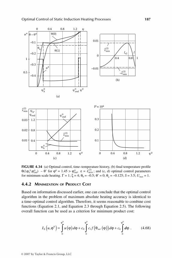
Optimal Control of Static Induction Heating Processes 187
4.4.2 MINIMIZATION OF PRODUCT COST
Based on information discussed earlier, one can conclude that the optimal controlalgorithm in the problem of maximum absolute heating accuracy is identical toa time-optimal control algorithm. Therefore, it seems reasonable to combine costfunctions (Equation 2.1, and Equation 2.3 through Equation 2.5). The followingoverall function can be used as a criterion for minimum product cost:
. (4.68)
FIGURE 4.34 (a) Optimal control, time–temperature history, (b) final temperature profileθ(l,ϕh
0,ϕend)0 – θ* for ϕ0 = 1.45 > ϕend,0 ε = ; and (c, d) optimal control parametersfor minimum scale heating. Γ = 1; ξ = 4; θ0 = –0.5; θ* = 0; θq = –0.125; S = 3.5; Umax = 1.
(a)
(c) (d)
(b)
0.1
0.2
0.3
I0 × 104
0
0.5
1
u∗
−0.1
−0.2
−0.3
−0.4
0.4 0.8 1.2 ϕ0
0.01
0.02
0.03
0.4
0.4
0.8
0.8
1.2
1.2 ϕ0 0.4 0.8 1.2 ϕ00
0
0.01
−0.01
1 0.4 0.8
θ − θ∗
u∗
θ(0)
ϕh0
ϕh,
ϕend
ϕh0
ϕ0end
ϕ0
ϕ0end
θ(1)θq
l le2
εmin∧(2)
εmin∧(2)
εmin∧(2)
−εmin∧(2)
εmin2( )
I u u d c c f d csur bΣ ,ϕ ϕ ϕ θ ϕ ϕϕ ϕ
0
0
0 1
0
0 0
( ) = ( ) + ( )( ) +∫ ∫ ddϕϕ
0
0
∫
DK6039_C004.fm Page 187 Thursday, June 8, 2006 12:34 PM
© 2007 by Taylor & Francis Group, LLC

188 Optimal Control of Induction Heating Processes
The first item in Equation (4.68) represents the cost function (Equation 2.3)that leads to minimization of the overall required energy. The second componenttakes into account the cost function (Equation 4.56 through Equation 4.57) thatminimizes metal loss due to scale formation. The third one describes expensesin Equation (2.5) due to given process time. Weighting coefficients c0 and cb makesense of a relative costing and represent an importance of each of the precedingconsidered items of the overall cost for a particular application. Coefficient c1
defines the relationship between the value of I in Equation (4.56) (calculated inrelative units) and the amount of scale during heating.
If the heating time, ϕ0, is fixed, then the value of cbϕ0 in Equation (4.68) isalso fixed a priori and the value of the cost function (Equation 4.68) dependsonly upon energy consumption and amount of scale.
Then it is sufficient to define the program of power variation during heating,which will minimize the following cost function:
. (4.69)
Let us consider the problem of cost minimization under conditions similarto Section 4.4.1. Cost function (Equation 4.56) will be replaced by criterion(Equation 4.69). The statement of the optimal control problem can be formulatedas follows. It is necessary to select such power control function u*(ϕ) boundedby the preassigned set in Equation (2.7) that provides steering workpiece initialtemperature distribution to desired temperature θ* with prescribed accuracy ε(according to Equation 2.25) for the given time ϕ0 and holds cost criterion(Equation 4.69) at extremum value.
Analysis of relative costing of cost function components in Equation (4.69)allows defining the shape of the optimal control input u*(ϕ).
If relative costing of metal loss due to scale in the product cost proves to beessential (i.e., when value of c0 is large enough), then the optimal control algo-rithm should contain the singular interval of the type in Equation (4.58). In thiscase, the optimal control algorithm with regard to target function (Equation 4.69)is identical by its nature to control algorithms, which are optimal with respect tominimum scale (Section 4.4.1.2). The additional calculation using the techniquedescribed in Section 4.4.1.2 leads to the same computational sets — for example,to the set in Equation (4.62). Because these sets always have a unique solution,we conclude that, under given values ε and ϕ0, the solution of the minimum costproblem is identical to the solution of the minimum scale problem.
If coefficient c0 in Equation (4.69) is small enough, then expenses due toenergy consumption can be considered as the main part of overall product costI∑. Therefore, optimal power control does not contain a singular control intervaland becomes identical to the algorithm that is optimal with respect to minimumenergy consumption. Analysis similar to that provided previously leads to the
I u I I u d c c fΣ ,ϕ ϕ ϕ θ ϕϕ ϕ
03 4
0
0 1
0
0 0
( ) = + = ( ) + ( )( )∫ sur∫∫ dϕ
DK6039_C004.fm Page 188 Thursday, June 8, 2006 12:34 PM
© 2007 by Taylor & Francis Group, LLC

Optimal Control of Static Induction Heating Processes 189
conclusion that, under given values ε and ϕ0, solution of the problem for mini-mizing cost function I∑ is identical to the solution of the minimum energyconsumption problem.
As a result, optimal with regard to overall cost I∑ control can be consideredas optimal by minimizing the scale formation or by minimizing energy consump-tion for each given pair of values ε and ϕ0. In the first case, the optimal algorithmcontains the singular interval (Section 4.4.1), but in the second case, only intervalswhere u*(ϕ) ≡ Umax and u*(ϕ) ≡ 0 (Section 2.9).
For given time ϕ0, two particular optimization problems can be solved forminimum scale or minimum energy consumption by using optimal control tech-niques that have been described earlier. Then it is possible to choose the soughtsolution of the initial minimum cost problem from obtained ones, which providessmaller value of overall cost function. The value of I∑(u*) can be calculated byExpression (4.68) in order to compare obtained solutions of separate optimizationproblems. Keep in mind that shapes of final spatial temperature distribution canbe different in these problems, as well as computational sets. Examples that havebeen provided in the previous section show that the continuous nature of depen-dency of the heating process parameters upon time ϕ0 leads to the same shapeof these curves as for the time-optimal control. With respect to minimum scaleformation, this conclusion does not remain valid for the problem of minimumenergy consumption.
Algorithms of heating power variation, which are optimal with respect totime and energy consumption criteria, have the same form (Equation 2.27) withalternating intervals of heating and temperature soaking (Section 2.9.2), but theirdurations ∆i
0 and in the general case do not coincide. This can leadto different profiles of final temperature distribution (Section 3.5). In particular,under < ε ≤ , the shapes of curves 0θ(l,∆1,∆2)
0 – θ* and θ(l, ) – θ*
(Figure 3.11 and Figure 3.17), and appropriate computational equation sets(Equation 3.12 and Equation 3.15; Equation 3.34 and Equation 3.35) differ fromeach other for the same value of ε.
Let us underline that the time required for heating with minimum energyconsumption is not fixed a priori. Its optimal value, ϕe
0, is calculated, aftercomputation of optimal values , as:
. (4.70)
Therefore, solution of this problem will comply with solution of the particularoptimization problem for this component of expenses in the overall cost, I∑, undercondition of fixed time, ϕ0, in the case when ϕ0 is equal to ϕe.
0 Obviously, if ϕ0
> ϕe,0 then the same result could be obtained by delaying the beginning of the
heating by ϕ0 – ϕe.0 If ϕ0 < ϕe,
0 then the new problem of minimum energy
∆i i N0 1, ,=
εmin( )2 εmin
( )1 ∆ ∆10
20,
∆i i N0 1, ,=
ϕe i
i
N
0 0
1
==∑∆
DK6039_C004.fm Page 189 Thursday, June 8, 2006 12:34 PM
© 2007 by Taylor & Francis Group, LLC

190 Optimal Control of Induction Heating Processes
consumption with predefined sum ϕ0 of all values would appear. Inthis case, the number of sought optimal control parameters decreases by one.
If the value of ϕ0 can be chosen freely under condition < ε ≤ , thendurations of two power constancy intervals of u*(ϕ) can be considered as twosought parameters. Because the sum of these parameters is a known fixed value,only one of them represents the single unknown variable. According to basicproperties (Equation 3.39 and Equation 3.40), the maximum deviation ε of finaltemperature from desired one is reached only at one point of the coordinate axis.
Similar analysis provided in Section 3.5, leads to the conclusion that thispoint will be located in the billet center l = 0. Figure 4.35 shows the shape oftemperature profile θ(l, )– θ*. An appropriate computational set of equa-tions can be reduced to the first equation of the set in Equation (3.35).
In the majority of typical cases, it is necessary to provide the best heatingaccuracy ε = attainable under the optimal control input that belongs to theclass of two-parameter functions. Consideration of these typical cases allowssimplifying the solution of the optimal control problem, which becomes optimalwith respect to minimum time or minimum energy consumption criteria (Section3.5). If given heating time ϕ0 in Equation (4.69) complies with minimum possibletime 0ϕmin( ) necessary to provide heating accuracy , then this controlfunction can be considered as optimal with respect to the cost function (Equation4.69) as well.
The following case will take place under condition ϕ0 > 0ϕmin( ). Theoptimal control can be defined as the two-parameter function that depends uponϕh and ϕend, according to Equation (4.61) or Equation (4.67), for required accuracyε = (ϕ0) when solving the particular optimization problem for minimum scale.
It is clear that, under ϕ0 = 0ϕmin( ), the value coincides with minimax, and the optimal control algorithm is defined by parameters ∆1
0 and ∆20
instead of parameters ϕh and ϕend. If the condition ϕ0 > 0ϕmin( ) is true, thenthe optimal algorithm of the type in Equation (4.61) and Equation (4.67) withsingular intervals of reduced power (Figure 4.30 and Figure 4.34) leads to smallerheating nonuniformity in comparison with (Figure 4.34c). However, in
FIGURE 4.35 Temperature profile at the end of the minimum energy heating process offixed duration ϕ0 < ϕe
0 for < ε ≤ .
0 1l
θ(l, ∆10, ∆0
2) − θ∗‒‒
ε
−ε
εmin( )2 εmin
( )1
∆i i N0 1, ,=
εmin( )2 εmin
( )1
∆ ∆10
20,
εmin( )2
εmin( )2 εmin
( )2
εmin( )2
ˆmin( )ε 2
εmin( )2 ˆ
min( )ε 2
εmin( )2
εmin( )2
ˆmin( )ε 2 εmin
( )2
DK6039_C004.fm Page 190 Thursday, June 8, 2006 12:34 PM
© 2007 by Taylor & Francis Group, LLC

Optimal Control of Static Induction Heating Processes 191
this case of ε = < , algorithms optimal by energy consumption usuallycomply with time-optimal algorithms (Section 3.5) and contain no less than threepower constancy intervals. In other words, under condition ϕ0 > 0ϕmin( )optimal by energy consumption heating modes that provide heating accu-racy, , do not correspond to the considered class of two-parameter controlinputs. Thus, one can conclude that the heat power control that is optimal byobjective function (Equation 4.69) minimizes metal loss due to scale formationas well.
Therefore, the optimal control problem should be solved (according to thetechnique described in Section 4.4.1.2) for each given value ϕ0 > 0ϕmin( ) andε = (ϕ0) with respect to cost functions (Equation 4.56 and Equation 4.57).The value of overall cost I∑ in Equation (4.68) can be calculated using controlinputs that have been found as a result of OCP solution.
Dependencies I∑(ϕ0) presented in Figure 4.36 correspond to a number ofvalues c0 > 0 and cb = 1 using results of optimal induction heating of steel billetswith respect to minimum scale (examples in Figure 4.31, Figure 4.32, and Figure4.34).1 The value of c1 = 2.8 ⋅ 104 ∆1
0 ( ) is determined for the case of metalloss that can be described by the parabolic law of oxidation in 0.5% of carboncomponent at ϕ0 = 0ϕmin( ).
Obtained curves allow one to find optimal heating time ϕopt0 that corresponds
to minimum value of I∑ under the condition that any value of ε = (ϕ0) canbe considered as satisfactory accuracy:
. (4.71)
Based on results shown in Figure 4.36, it is possible to conclude that conditionϕopt
0 = 0ϕmin( ) is true for all values c0 ≤ c0* = 0.15. Therefore, the time-optimal
process proves to be optimal with respect to minimum product cost under the
FIGURE 4.36 Minimum product cost as a function of process time. Γ = 1; ξ = 4; θ0 =–0.5; θ* = 0; θq = –0.125; S = 3.5; ε0 = ; Umax = 1.
ˆmin( )ε 2 εmin
( )2
εmin( )2
ˆmin( )ε 2
εmin( )2
ˆmin( )ε 2
εmin( )2
εmin( )2
ˆmin( )ε 2
ϕ ϕ ϕ ϕ εϕ
optu
I u0 0 0 0 2
0= ( )( ) ≥ ( )( )min min , , min minΣ ,, ˆ
minε ε ϕ= ( )( )2 0
εmin( )2
0.3 0.4 0.6 0.80.5 0.7 0.9 1.0 ϕ0
0.6
0.8
1.0
1.2
1.4
IΣ
1.0
0.6
0.150.3
C0 = 1.5
ϕmin0
ˆmin( )ε 2
DK6039_C004.fm Page 191 Thursday, June 8, 2006 12:34 PM
© 2007 by Taylor & Francis Group, LLC
192 Optimal Control of Induction Heating Processes
appropriate values of c0. For c0 > c0*, the minimum product cost is reached under
control, minimizing metal loss due to scale, for any value of process time.The control algorithm, which provides minimum energy consumption, under
particular conditions would result in minimum product cost. This algorithm canbe found using the computational procedure described above with neglectedrestraint on the value of admissible temperature deviation. Control input shouldbe considered in the class of N-parameter functions (N > 2).
4.5 OPTIMAL CONTROL OF MULTIDIMENSIONAL LINEAR MODELS OF INDUCTION HEATING PROCESSES
Most mathematical models of induction heating tend to be handled with a com-bination of the following assumptions (Section 2.3):
• Neglecting nonlinearity by averaging process parameters on appropri-ate temperature intervals;
• Concentrating on considering of regular-shaped workpieces (i.e., plate,cylinder, rectangle slab, parallelepiped, sphere);
• Simplifying the description of the geometric input data for the induc-tion heating system;
• Taking into account the nonuniformity of temperature distribution onlyalong one or two coordinates (reducing the three-dimensional temper-ature field to one-dimensional or two-dimensional forms).
The linear one-dimensional model as a basic model of induction heating ofregular-shaped bodies has been considered in previous chapters. This simplifiedmodel describes one-dimensional processes of heat transfer along the thicknessof an infinitely long plate or along the radius of an infinite length cylinder. It hasbeen assumed that temperature nonuniformity along other coordinates can beneglected. The last assumption does not lead to substantial errors in some con-ventional induction heating applications because of inessential nonuniformity ofheat source distribution along the workpiece length and relatively small heat lossfrom butt ends of the heated body.
However, these assumptions do not provide an accurate enough descriptionof electromagnetic and temperature fields in many practical applications. Inparticular, electromagnetic end and edge effects and the field distortion causedby them are primarily responsible for nonuniform temperature profiles in cylin-drical, and rectangular workpieces. Due to the great importance of these effectsin induction heating applications, multidimensional models of heating processesshould be used.15,16 For the majority of practical problems, the temperature dis-tribution within the heated cylindrical billet can be considered accurately enoughas an axially symmetrical temperature field.
DK6039_C004.fm Page 192 Thursday, June 8, 2006 12:34 PM
© 2007 by Taylor & Francis Group, LLC
Optimal Control of Static Induction Heating Processes 193
On the other hand, the temperature distribution along the length of the slabcan be assumed as uniform. Therefore, depending upon the particular inductionheating process, two-dimensional mathematical models can be effectively usedto describe nonuniform temperature distribution of the heated workpiece (1) alongaxial and radial directions of a cylinder of finite length and (2) in the plane ofthe cross-section of the heated slab that can be considered as an infinitely longplate.
This chapter discusses the time-optimal control problem utilizing two-dimen-sional models of induction heating processes. An ability to extend obtained resultsto solution of other optimization problems will be investigated here as well asconsideration of all essential features of real-life processes.
4.5.1 LINEAR TWO-DIMENSIONAL MODEL OF THE INDUCTION HEATING PROCESS
Let us consider the general optimal control problem assuming that completeinformation is available with respect to the heating process and imposed require-ments. Let us also assume that there are no disturbances affecting the heatingsystem and the time of workpiece transfer to hot working equipment can beneglected. The function θ(l,y,ϕ) will be treated as an output-controlled functionof the process that describes nonuniform temperature distribution in axial/radialdirections of a cylindrical billet of finite length or within a cross-section of therectangular-shaped workpiece (rectangular slab of infinite length). The followingtwo-dimensional linear equation of heat transfer will be considered further as abasic mathematical model of the induction heating process1:
,
(4.72)
Equation (4.72) is written with respect to relative (dimensionless) units. Initial and boundary conditions of the second kind can be formulated as:
θ(l,y,0) = θ0(l,y); l ∈ [0,1]; y ∈ [0,1]; (4.73)
(4.74)
∂ ( )∂
=∂ ( )
∂+
∂ ( )∂
+∂θ ϕ
ϕθ ϕ θ ϕ
βl y l y
l l
l y
l
, , , , , ,2
22Γ 22
2
0 1 0
θ ϕξ ϕ
l y
yW l y u
l y
d, ,
, , ,
;
( )∂
+ ( ) ( )
< < < < < ≤1 0 0; ϕ ϕ
∂ ( )∂
= ( ) ∂ ( )∂
=
∂ ( )
θ ϕϕ
θ ϕ
βθ ϕ
1 00
1
, ,, ;
, ,;
, ,
y
lq y
y
l
l
∂∂= ( ) ∂ ( )
∂= − ( )
∈
yq l
l
yq l
l
T T1 00
0 1
, ;, ,
,
[ , ]
ϕ βθ ϕ
ϕΓ
;; [ , ]; .y ∈ < ≤0 1 0 0ϕ ϕ
DK6039_C004.fm Page 193 Thursday, June 8, 2006 12:34 PM
© 2007 by Taylor & Francis Group, LLC
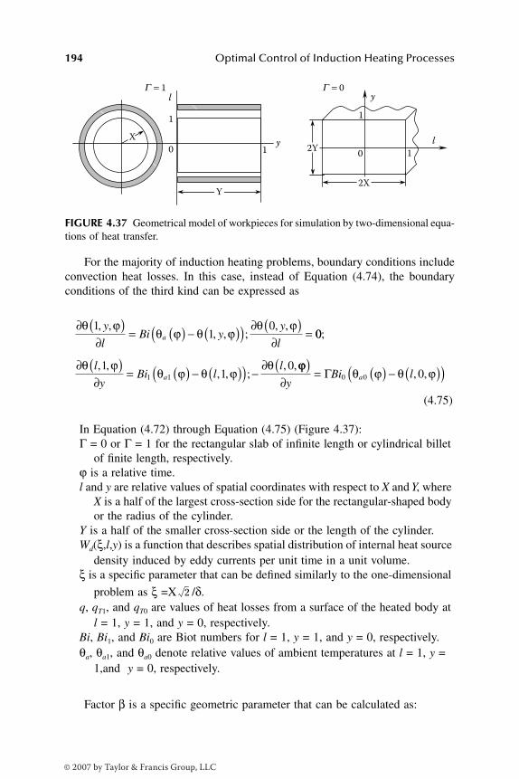
194 Optimal Control of Induction Heating Processes
For the majority of induction heating problems, boundary conditions includeconvection heat losses. In this case, instead of Equation (4.74), the boundaryconditions of the third kind can be expressed as
(4.75)
In Equation (4.72) through Equation (4.75) (Figure 4.37):Γ = 0 or Γ = 1 for the rectangular slab of infinite length or cylindrical billet
of finite length, respectively.ϕ is a relative time.l and y are relative values of spatial coordinates with respect to X and Y, where
X is a half of the largest cross-section side for the rectangular-shaped body or the radius of the cylinder.
Y is a half of the smaller cross-section side or the length of the cylinder.Wd(ξ,l,y) is a function that describes spatial distribution of internal heat source
density induced by eddy currents per unit time in a unit volume.ξ is a specific parameter that can be defined similarly to the one-dimensional
problem as ξ =X /δ.q, qT1, and qT0 are values of heat losses from a surface of the heated body at
l = 1, y = 1, and y = 0, respectively.Bi, Bi1, and Bi0 are Biot numbers for l = 1, y = 1, and y = 0, respectively.θa, θa1, and θa0 denote relative values of ambient temperatures at l = 1, y =
1,and y = 0, respectively.
Factor β is a specific geometric parameter that can be calculated as:
FIGURE 4.37 Geometrical model of workpieces for simulation by two-dimensional equa-tions of heat transfer.
X
Y
0 1y
y
1
l
l
G = 1 G = 0
1
1
02Y
2X
∂ ( )∂
= ( ) − ( )( ) ∂ ( )∂
=θ ϕ
θ ϕ θ ϕθ ϕ1
10, ,
, , ;, ,y
lBi y
y
la 00
11
01 1
;
, ,, , ;
, ,∂ ( )∂
= ( ) − ( )( ) −∂θ ϕ
θ ϕ θ ϕθl
yBi l
la
ϕϕθ ϕ θ ϕ( )
∂= ( ) − ( )( )
yBi laΓ 0 0 0, ,
2
DK6039_C004.fm Page 194 Thursday, June 8, 2006 12:34 PM
© 2007 by Taylor & Francis Group, LLC

Optimal Control of Static Induction Heating Processes 195
β = X/Y. (4.76)
Other relative values can be calculated from corresponding formulas similar tothose used in Chapter 1. The value of X can be considered as a basic spatialcoordinate.
Equation (4.72) through Equation (4.75) describe two-dimensional tempera-ture distribution θ(l,y,ϕ) at any time and at any point with coordinates l and y.The heating process is caused by internally generated heating power representedby function Wd(ξ,l,y)u(ϕ). The initial temperature state θ0(l,y) in Equation (4.73)refers to the fixed temperature distribution within the workpiece at time ϕ = 0.
The boundary conditions in Equation (4.74) or Equation (4.75) for Γ = 1determine the value of heat losses from the butt-end and lateral surfaces of thebillet and allow consideration of the cylindrical billet as an axially symmetricalbody (l = 0 is the axis of symmetry). In the general case, heat losses from asurface of the heated body can be specified by values q(y,ϕ), qT1(l,ϕ), and qT0(l,ϕ)in Equation (4.74). For heat transfer by convection, the boundary conditionsinclude Biot numbers Bi, Bi1, and Bi0. Appropriate ambient temperatures inEquation (4.75) will be equal respectively to θa, θa1, and θa0. The center of cross-section should be taken as the coordinate origin in simulation of the heatingprocess for the rectangular slab (Γ = 0). Therefore, it is beneficial to take advan-tage of symmetry and consider only the temperature field distribution within aquarter of the workpiece cross-section.
According to the symmetry condition, the temperature gradient in Equation(4.74) will be equal to zero at l = 1 and y = 0 (Figure 4.37). Therefore, anexpression, β > 1, remains valid for Equation (4.76) because the value of Xrepresents a length of the largest half-side of the rectangular cross-section. Time-dependent heating power u(ϕ) is chosen as a lumped control input constrainedby Equation (2.7).
The relatively complicated two-dimensional electromagnetic problem shouldbe solved to determine the function Wd (ξ,l,y) in Equation (4.72).15,16 Approximateanalytical expressions can be used for simulation of function Wd (ξ,l,y). At thesame time, numerical models allow representing the function Wd (ξ,l,y) as a two-dimensional mesh function. Similarly to Equation (1.36), solution of the problemin Equation (4.72) under boundary conditions in Equation (4.73) and Equation(4.74) or Equation (4.73) and Equation (4.75) can be written in the form of theDuhamel integral as1:
. (4.77)
Functions Φ(l,y,ϕ) and Λ(l,y,ϕ) can be calculated taking into considerationappropriate boundary conditions of the second (Φ2,Λ2) and the third (Φ3,Λ3) kindsas1:
θ ϕ ϕϕ τ
ϕτ τ
ϕ
l y l yl y
u d, , , ,, ,( ) = ( ) + ∂ −( )∂
( )∫ΦΛ
0
DK6039_C004.fm Page 195 Thursday, June 8, 2006 12:34 PM
© 2007 by Taylor & Francis Group, LLC

196 Optimal Control of Induction Heating Processes
(4.78)
(4.79)
(4.80)
.
(4.81)
In Expression (4.78) through Equation (4.81):
Φ Γ Γ2 000 002
0
1 1
2
l y g d, , *ϕ θ τ τϕ
( ) = +( ) + +( ) ( ) +
+
( )∫KK l
Ke gr
rr
r rr
µµ
θ τµ ϕ
ϕ( )( ) ⋅ + ( )
=
∞− ( )∑ ∫2
1
0 0 02
0
2 * ee d
e g
r
nn
− −( )
−
+
+ +( ) +
µ ϕ τ
β λ ϕ
τ
θ
2
2 2
2 1 00Γ 002
01
2 2
n
n
e d Kn* *( ) − −( )
=
∞
∫∑ ( )
⋅
ϕβ λ ϕ ττ τ λλ
µ λµ
θ
n
r n
rnr
rn
y
K l K y
Ke
( ) +
+ ( ) ( )( )
=
∞
=
∞
∑∑2 2
11
0
*−− +( ) ( ) − +( ) −
+ ( )∫µ β λ ϕϕ
µ β λ ϕτr n r n
g ern
2 2 2 2 2 22
0
* τττ( )
d ;
Φ3
11
0
2 2 2
l y D e grn
nr
rnr n
, ,ϕ θµ β λ ϕ( ) = +
=
∞
=
∞− +( )∑∑ rrn e d
r n* 3
0
2 2 2( ) − +( ) −( )∫ ( )
×
×
ϕµ β λ ϕ τ
τ τ
KK l K yr nµ λ( ) ( )*
Λ Γ2 000
1 2l y U W UW K lr r
, , max maxϕ ξ ϕξ µ( ) = +( ) ( ) +( ) ( ))
( ) ⋅ −
+
+ +( )
−
−
∞
∑ µ µµ ϕ
r rrK
e
UW
r2 2
1
0
1
2 1
2
max Γ nn n
nn
K l ye
U
nξβ λ
β λ ϕ( ) ( )−
+
+
−
=
∞
∑*
max
2 2
1
1
4
2 2
WW K l K y
Ke
rn r n
r n r
ξ µ λµ β λ µ
µ( ) ( ) ( )+( ) ( )
−−
* *
2 2 2 21
rr n
nr
2 2 2
11
+( )=
∞
=
∞
∑∑ β λ ϕ;
Λ3 2 2l y UD W K l K yrn rn r n
r
, , max
*
ϕξ µ λµ β λ
( ) = ( ) ( ) ( )+ nnnr
er n
2
11
12 2 2
−
− +( )=
∞
=
∞
∑∑ µ β λ ϕ
DK6039_C004.fm Page 196 Thursday, June 8, 2006 12:34 PM
© 2007 by Taylor & Francis Group, LLC
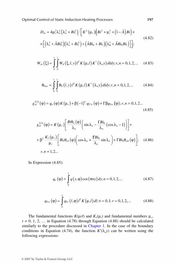
Optimal Control of Static Induction Heating Processes
197
(4.82)
(4.83)
(4.84)
(4.85)
(4.86)
In Expression (4.85):
(4.87)
(4.88)
The fundamental functions
K
(
µ
rl
) and
K
1
(
µ
r
) and fundamental numbers
µ
r
,
r
= 0, 1, 2, … in Equation (4.78) through Equation (4.88) should be calculatedsimilarly to the procedure discussed in Chapter 1. In the case of the boundaryconditions in Equation (4.74), the function
K
*
(
λ
n
y
) can be written using thefollowing expressions:
D Bi K Bi A Birn r n n r r= +( ) ( ) + + −( )4 12 2 212 2 2 2µ λ λ µ µ (( )
×
× +( ) +( ) + +( )λ λ λn nABi Bi ABi Bi202 2
12
0 1
nn ABi Bi20 1+( )
;
W W l y l K l K y dldy rrn d r nξ ξ µ λ( ) = ( ) ( ) ( )∫∫0
1
0
1
, , ;*Γ ,, , , , ...n = 0 1 2
θ θ µ λ0 0
0
1
0
1
0rn r nl y l K l K y dldy r n= ( ) ( ) ( ) =∫∫ , ; ,*Γ ,, , , ...1 2
g q K q qrn n rn
T r Tor* 2
11( ) ( ) = ( ) ( ) + −( ) ( ) +ϕ ϕ µ β ϕ β ϕΓ (( ) =; , , , ...r n 0 1 2
g KBi Bi
rn ra
nn
nn
* sin cos3 0( ) ( ) = ( ) ( ) − −ϕ µθ ϕλ
λλ
λΓ11
2 11 1
( )
+
+ ( ) ( ) +βµ
µθ ϕ λ
KBir
ra ncos
ΓΓ ΓBiBi
r n
nn a
00 0
1 2
λλ θ ϕsin ;
, ,
+ ( )
= ....
q q y ny dy nn ϕ ϕ π( ) = ( ) ( ) =∫0
1
0 1 2, cos ; , , , ...
q q l l K l dl rTvr Tv rϕ ϕ µ ν( ) = ( ) ( ) = =∫0
1
0 1 0 1 2, ; , ; , ,Γ ,, ...
DK6039_C004.fm Page 197 Friday, June 9, 2006 8:07 AM
© 2007 by Taylor & Francis Group, LLC
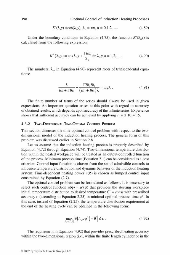
198 Optimal Control of Induction Heating Processes
K*(λny) =cos(λny), λn = πn, n = 0,1,2, .... (4.89)
Under the boundary conditions in Equation (4.75), the function K*(λny) iscalculated from the following expression:
. (4.90)
The numbers, λn, in Equation (4.90) represent roots of transcendental equa-tions:
. (4.91)
The finite number of terms of the series should always be used in givenexpressions. An important question arises at this point with regard to accuracyof obtained results, which depends upon accuracy of the infinite series. Experienceshows that sufficient accuracy can be achieved by applying r, n ≤ 10 ÷ 15.
4.5.2 TWO-DIMENSIONAL TIME-OPTIMAL CONTROL PROBLEM
This section discusses the time-optimal control problem with respect to the two-dimensional model of the induction heating process. The general form of thisproblem was discussed earlier in Section 2.8.
Let us assume that the induction heating process is properly described byEquation (4.72) through Equation (4.74). Two-dimensional temperature distribu-tion within the heated workpiece will be treated as an output-controlled functionof the process. Minimum process time (Equation 2.1) can be considered as a costcriterion. Control input function is chosen from the set of admissible controls toinfluence temperature distribution and dynamic behavior of the induction heatingsystem. Time-dependent heating power u(ϕ) is chosen as lumped control inputconstrained by Equation (2.7).
The optimal control problem can be formulated as follows. It is necessary toselect such control function u(ϕ) = u*(ϕ) that provides the steering workpieceinitial temperature distribution to desired temperature θ* = const with prescribedaccuracy ε (according to Equation 2.25) in minimal optimal process time ϕ0. Inthis case, instead of Equation (2.25), the temperature distribution requirement atthe end of the heating cycle can be obtained in the following form:
. (4.92)
The requirement in Equation (4.92) that provides prescribed heating accuracywithin the two-dimensional region (i.e., within the finite length cylinder or in the
K y yBi
y nn nn
n* cos sin , , , ...λ λ
λλ( ) = + =Γ 0 1 2
λλ
λBi Bi
Bi Bi
Bi Bictg
1 0
0 1
1 0+−
+( ) =Γ
Γ
max , ,, ,
*
l yl y
∈[ ] ( ) − ≤0 1
0θ ϕ θ ε
DK6039_C004.fm Page 198 Thursday, June 8, 2006 12:34 PM
© 2007 by Taylor & Francis Group, LLC
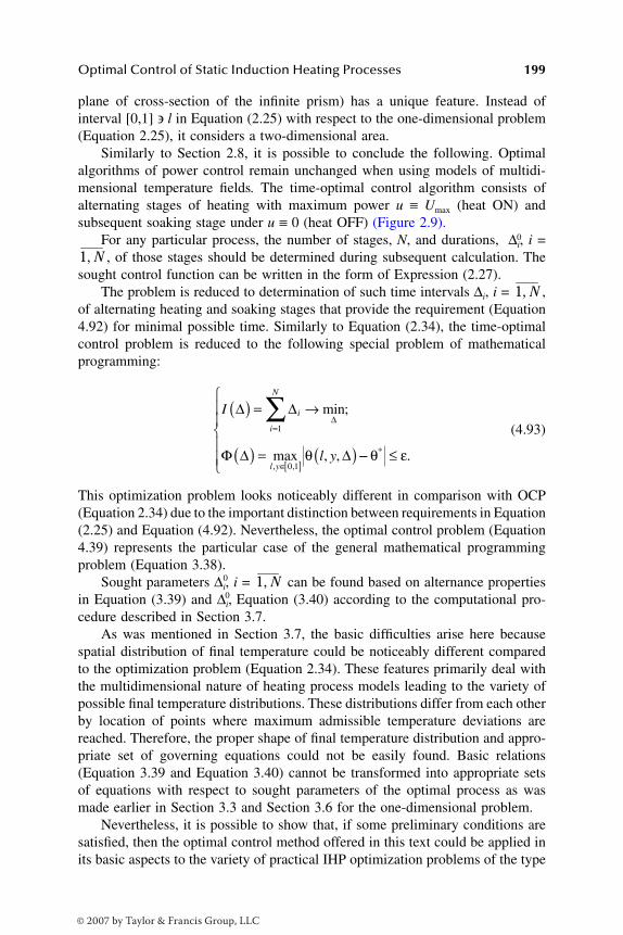
Optimal Control of Static Induction Heating Processes 199
plane of cross-section of the infinite prism) has a unique feature. Instead ofinterval [0,1] ∋ l in Equation (2.25) with respect to the one-dimensional problem(Equation 2.25), it considers a two-dimensional area.
Similarly to Section 2.8, it is possible to conclude the following. Optimalalgorithms of power control remain unchanged when using models of multidi-mensional temperature fields. The time-optimal control algorithm consists ofalternating stages of heating with maximum power u ≡ Umax (heat ON) andsubsequent soaking stage under u ≡ 0 (heat OFF) (Figure 2.9).
For any particular process, the number of stages, N, and durations, 0∆i, i =, of those stages should be determined during subsequent calculation. The
sought control function can be written in the form of Expression (2.27).The problem is reduced to determination of such time intervals ∆i, i = ,
of alternating heating and soaking stages that provide the requirement (Equation4.92) for minimal possible time. Similarly to Equation (2.34), the time-optimalcontrol problem is reduced to the following special problem of mathematicalprogramming:
(4.93)
This optimization problem looks noticeably different in comparison with OCP(Equation 2.34) due to the important distinction between requirements in Equation(2.25) and Equation (4.92). Nevertheless, the optimal control problem (Equation4.39) represents the particular case of the general mathematical programmingproblem (Equation 3.38).
Sought parameters ∆i,0 i = can be found based on alternance properties
in Equation (3.39) and ∆i,0 Equation (3.40) according to the computational pro-
cedure described in Section 3.7.As was mentioned in Section 3.7, the basic difficulties arise here because
spatial distribution of final temperature could be noticeably different comparedto the optimization problem (Equation 2.34). These features primarily deal withthe multidimensional nature of heating process models leading to the variety ofpossible final temperature distributions. These distributions differ from each otherby location of points where maximum admissible temperature deviations arereached. Therefore, the proper shape of final temperature distribution and appro-priate set of governing equations could not be easily found. Basic relations(Equation 3.39 and Equation 3.40) cannot be transformed into appropriate setsof equations with respect to sought parameters of the optimal process as wasmade earlier in Section 3.3 and Section 3.6 for the one-dimensional problem.
Nevertheless, it is possible to show that, if some preliminary conditions aresatisfied, then the optimal control method offered in this text could be applied inits basic aspects to the variety of practical IHP optimization problems of the type
1 N,
1 N,
I
l y
i
i
N
l y
∆ ∆
Φ ∆ ∆
∆( ) = →
( ) = ( )=
∈[ ]
∑1
0 1
min;
max , ,, ,
θ −− ≤
θ ε* .
1 N,
DK6039_C004.fm Page 199 Thursday, June 8, 2006 12:34 PM
© 2007 by Taylor & Francis Group, LLC
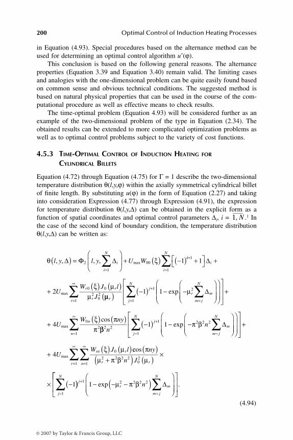
200 Optimal Control of Induction Heating Processes
in Equation (4.93). Special procedures based on the alternance method can beused for determining an optimal control algorithm u*(ϕ).
This conclusion is based on the following general reasons. The alternanceproperties (Equation 3.39 and Equation 3.40) remain valid. The limiting casesand analogies with the one-dimensional problem can be quite easily found basedon common sense and obvious technical conditions. The suggested method isbased on natural physical properties that can be used in the course of the com-putational procedure as well as effective means to check results.
The time-optimal problem (Equation 4.93) will be considered further as anexample of the two-dimensional problem of the type in Equation (2.34). Theobtained results can be extended to more complicated optimization problems aswell as to optimal control problems subject to the variety of cost functions.
4.5.3 TIME-OPTIMAL CONTROL OF INDUCTION HEATING FOR CYLINDRICAL BILLETS
Equation (4.72) through Equation (4.75) for Γ = 1 describe the two-dimensionaltemperature distribution θ(l,y,ϕ) within the axially symmetrical cylindrical billetof finite length. By substituting u(ϕ) in the form of Equation (2.27) and takinginto consideration Expression (4.77) through Expression (4.91), the expressionfor temperature distribution θ(l,y,∆) can be obtained in the explicit form as afunction of spatial coordinates and optimal control parameters ∆i, i = .1 Inthe case of the second kind of boundary condition, the temperature distributionθ(l,y,∆) can be written as:
(4.94)
1 N,
θ ξl y l y U Wi
i
N
, , , , max∆ Φ ∆( ) =
+ ( ) −( )
=∑2
1
00 1ii
i
N
i
r r
r
UW J l
J
+
=
+
+
+( ) ( )
∑ 1
1
0 0
202
1
2
∆
max
ξ µµ µµ
µrr
jr m
m j
N
( ) −( ) − −
=
∞+
=∑ ∑
1
1 21 1 exp ∆
+
+( ) ( )
=∑
j
N
nU
W ny
1
0
24 max
cosξ ππ ββ
π β2 2
1
1 2 2 21 1n
nn
jm
m j
N
=
∞+
=∑ ∑−( ) − −
exp ∆
+
+( ) ( )
=∑
j
N
rn rU
W J l
1
04 max
ξ µ ccos πµ π β µ
ny
n Jr rnr
( )+( ) ( )
×
× −(
=
∞
=
∞
∑∑ 2 2 2 202
11
1)) − − −( )
+
==∑∑ j
r m
m j
N
j
N
n1 2 2 2 2
1
1 exp µ π β ∆
.
DK6039_C004.fm Page 200 Thursday, June 8, 2006 12:34 PM
© 2007 by Taylor & Francis Group, LLC

Optimal Control of Static Induction Heating Processes 201
In the case of the third kind of boundary condition, it can be calculated usingthe following expression:
(4.95)
In contrast to one-dimensional models, nonuniformity of electromagnetic heatsource distribution along the workpiece length and heat losses from the workpiecebutt ends (y = 1 and y = 0) and lateral (l = 1) surfaces now will be taken into account.
The field distortion caused by these effects is primarily responsible for quan-titative variation of radial temperature distribution within the heated cylindricalbillet. However, in many practical cases such effects cause relatively small tem-perature gradients in the axial direction. Therefore, an existence of those effectsdoes not lead to qualitative change of the shape of final radial temperaturedistribution in any cross-section of the cylinder.
The number of extremum points of the curve θ (l,y,ϕ0) under y = const canbe determined according to the relationship in Equation (3.10). This conditiondirectly links the number, N, of control intervals with the number of extremumpoints, Mmax. This fact was already discussed in Chapter 3. The area with maxi-mum and minimum temperatures will be located at some internal points xj
0 =(lj
0,yj0) within cylinder cross-sections. Axial coordinate yj
0 specifies location ofcross-sections where the points xj
0 = (lj0,yj
0) should be found.If axial temperature distribution is nonuniform, then points xj
0 will be locatedin different cylinder cross-sections that represent the unique feature of the two-dimensional problem. All possible scenarios of location of points 0xj, j = could not be unambiguously set a priori. Therefore, the set of governing equationsalso could not be easily found for prescribed value ε in Equation (4.93). Thisadds complexity to solution of the two-dimensional time-optimal control problemof induction heating of cylindrical billets.
Because general equalities (Equation 3.39 and Equation 3.40) remain valid,in this case analogies with the one-dimensional problem can be used. Finaltemperature distribution θ(l,y,∆0) and all optimal process parameters ∆i
0 can berepresented as continuous functions of ε. Under given conditions, it is possibleto obtain the following results1 (similar to Section 3.7).
1. If heating accuracy satisfies equality ε = , then condition N = 1will be valid. This means that time-optimal heating represents a single-stage process utilizing maximum power. We shall limit our consider-ation to the typical case of heating accuracy > εinf that corresponds
θµ
l y l y U
D J l
i
i
N rn r
, , , , max∆ Φ ∆( ) =
+
( )
=∑3
1
0 ccos sinλλ
λ
µ β λ
nn
n
r nnr
yBi
y+
+( )=
∞
=∑
0
2 2 2111
1
1
2 2 21 1
∞
+
=
∑
∑
×
× ( ) −( ) − − −( )Wrnj
j
N
r n iξ µ β λexp ∆mm j
N
=∑
.
1 R,
εmin( )1
εmin( )1
DK6039_C004.fm Page 201 Thursday, June 8, 2006 12:34 PM
© 2007 by Taylor & Francis Group, LLC

202 Optimal Control of Induction Heating Processes
to substantially small heat losses from a surface of the heated body. Inthis case, the minimum admissible temperatures will be reached in thecore of the billet at the end of the time-optimal single-stage heatingcycle that provides the best heating accuracy . At the same time,the region with maximum temperature will be located at a certaininternal point (subsurface region) within the heated billet (see Figure3.6 and Section 3.3). The temperature of the lateral surface (l = 1) inany cylinder cross-section remains within admissible limits. The tem-perature of the butt-end surface will be lower than maximum admissiblelevel due to heat losses. This means that, for ε = , there will be only a single possibletemperature distribution θ(l,y,∆0) (Figure 4.38) that is characterizedaccording to Equation (3.39) and Equation (3.40) by two extremumpoints xj
0 = (lj0,yj
0); j = 1, 2. Both points represent maximum admissibledeviations of final temperature from the required one. In this case,minimum and maximum temperatures will be reached in the core ofthe cylinder (l1
0 = 0, y10) and at some internal point (l2
0 = le2, y20 = ye2),
respectively.It is feasible to determine only the set of possible variants of temper-ature distribution θ(l,y,∆0). Every variant would correspond only to aparticular case. Mainly, it is impossible to select a priori the singlevariant from this set for each particular case.Minimum temperature can be positioned in three different locationson the cylinder axis. Its location primarily depends upon correlationbetween the value of heat loss from the butt-end surface and heat sourcedistribution along the billet length. A relatively small coil overhangrepresents the typical case. In this case, the surface density of internalheat generation can be considered as uniformly distributed along theaxis, y, or as reducing toward the butt-ends of the billet.15 Two pointswith minimum final temperature can be located on the cyclinder axisl = 0 within butt-ends y1
0 =0 or y10 =1. Figure 4.38a and Figure 4.38b
FIGURE 4.38 Variants of location of minimum and maximum temperature points at theend of time-optimal heating of finite length cylindrical billet for ε = .
1
x02(max) x0
2(max) x0
2(max)
x01(min)x0
1(min) x0
1(min)
0 1
(a)
y
le2
ye2 1
(b)
yye2 1
(c)
yye2
l
1
0
le2
l
1
0
le2
l
εmin( )1
εmin( )1
εmin( )1
DK6039_C004.fm Page 202 Thursday, June 8, 2006 12:34 PM
© 2007 by Taylor & Francis Group, LLC

Optimal Control of Static Induction Heating Processes 203
show these variants for minimum temperature points (l10 = 0, y1
0 = 0)and (l1
0 = 0, y10 = 1), respectively.
With increase of the coil overhang, the power of internal heat genera-tion at the billet butt-ends grows in comparison with internal cross-sections of the billet.15 Then, minimum temperature can be located ata certain point on the axis (l1
0 = 0) with coordinate y that satisfiescondition 0 < y1
0 < 1 (Figure 4.38c). Similarly to Equation (3.12),Expression (3.39) and Expression (3.40) can be transformed into thefollowing set of equations:
(4.96)
Observation that the temperature gradient is equal to zero at the extre-mum point can be used in the form of the last equality in Equation(4.96). This will allow one to define unknown coordinates le2 and ye2.As one can see, this equality is similar to condition ∂θ(le2,∆0)/∂l = 0in Equation (3.12).Assuming that the point of minimum temperature is located on thebillet’s axis, the set in Equation (4.96) should be supplemented by oneof the following equations:
. (4.97)
The proper choice of a single equality can be done according to thegiven value of the coil overhang and based on correlation betweenvalues of qT1 and qT0 (or Bi1, θa1, and Bi0, θa0) in Equation (4.74) orEquation (4.75). Further computation of the optimal process validatesthe chosen variant if minimum temperature will be reached at one ofthe considered points. Otherwise, the point (0,y1
0) should be consideredas the point where temperature minimum will be located.After substitution of θ(l,y,∆0) in the form of Equation (4.94) or Equation(4.95) into the set of Equation (4.96) and Equation (4.97), this set canbe solved with respect to five unknown variables: 0∆1, , le2, ye2, andy1.
0 If equalities y10 = 0 or y1
0 = 1 could be set a priori, the set (Equation4.96) can be solved with respect to four unknown variables: ∆1,
0 ,
θ θ ε
θ θ
0 10
10 1
2 2 10
, , ;
,
*min
,*
y
l ye e
∆
∆
( ) − = −
( ) − =
( )
++
∂ ( )∂
=∂ ( )
( )ε
θ θ
min
, ,
;
, ,
1
2 2 10
2 2 10l y
l
l ye e e e∆ ∆∂∂
=
y
0.
y yy
y10
10 1
010
0 10
0= =∂ ( )
∂=; ;
, ,θ ∆
εmin( )1
εmin( )1
DK6039_C004.fm Page 203 Thursday, June 8, 2006 12:34 PM
© 2007 by Taylor & Francis Group, LLC
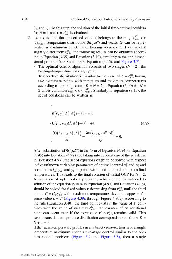
204 Optimal Control of Induction Heating Processes
le2, and ye2. At this step, the solution of the initial time-optimal problemfor N = 1 and ε = is obtained.
2. Let us assume that prescribed value ε belongs to the range < ε< . Temperature distribution θ(l,y,∆0) and vector ∆0 can be repre-sented as continuous functions of heating accuracy ε. If values of εslightly differ from , the following results can be obtained accord-ing to Equation (3.39) and Equation (3.40), similarly to the one-dimen-sional problem (see Section 3.3, Equation (3.15), and Figure 3.7):• The optimal control algorithm consists of two stages (N = 2): the
heating–temperature soaking cycle.• Temperature distribution is similar to the case of ε = having
two extremum points with minimum and maximum temperaturesaccording to the requirement R = N = 2 in Equation (3.40) for N =2 under condition < ε < . Similarly to Equation (3.15), theset of equations can be written as:
(4.98)
After substitution of θ(l,y,∆0) in the form of Equation (4.94) or Equation(4.95) into Equation (4.98) and taking into account one of the equalitiesin (Equation 4.97), the set of equations ought to be solved with respectto five unknown variables: parameters of optimal control ∆1
0 and 0∆2 andcoordinates le2, ye2, and y1
0 of points with maximum and minimum finaltemperatures. This leads to the final solution of initial OCP for N = 2.A sequence of optimization problems, which could be reduced tosolution of the equation system in Equation (4.97) and Equation (4.98),should be solved for fixed values ε decreasing from until the thirdpoint, x3
0 = 0(l3,y3),0 with maximum temperature deviation appears for
some value ε = ε* (Figure 4.39a through Figure 4.39c). According tothe rule (Equation 3.40), the third point exists if the value of ε* coin-cides with the value of minimax . Appearance of an additionalpoint can occur even if the expression ε* > remains valid. Thiscase means that temperature distribution corresponds to condition R =N + 1 = 3.If the radial temperature profiles in any billet cross-section have a singletemperature maximum under a two-stage control similar to the one-dimensional problem (Figure 3.7 and Figure 3.8), then a single
εmin( )1
εmin( )2
εmin( )1
εmin( )1
εmin( )1
εmin( )2 εmin
( )1
θ θ ε
θ θ
0 10
10
20
2 2 10
20
, , , ;
, ,
*
,
y
l ye e
∆ ∆
∆ ∆
( ) − = −
( ) − **
, ,
;
, , , ,
= +
∂ ( )∂
=∂
ε
θ θl y
l
l ye e e e2 2 10
20
2 2 10∆ ∆ ∆ ∆22
0
0( )
∂=
y
.
εmin( )1
εmin( )2
εmin( )2
DK6039_C004.fm Page 204 Thursday, June 8, 2006 12:34 PM
© 2007 by Taylor & Francis Group, LLC
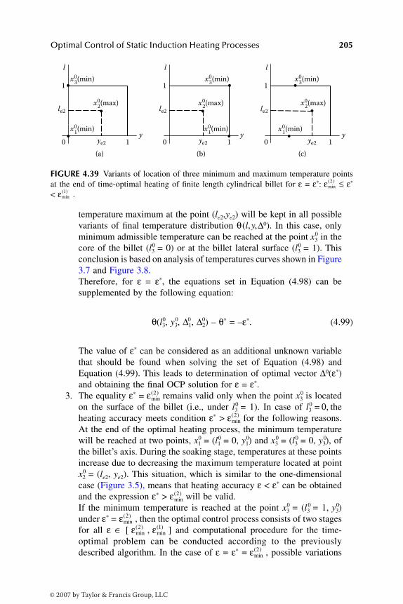
Optimal Control of Static Induction Heating Processes 205
temperature maximum at the point (le2,ye2) will be kept in all possiblevariants of final temperature distribution θ(l,y,∆0). In this case, onlyminimum admissible temperature can be reached at the point x3
0 in thecore of the billet (l3
0 = 0) or at the billet lateral surface (l30 = 1). This
conclusion is based on analysis of temperatures curves shown in Figure3.7 and Figure 3.8.Therefore, for ε = ε*, the equations set in Equation (4.98) can besupplemented by the following equation:
θ(l3,0 y3,
0 ∆1,0 ∆2)
0 – θ* = –ε*. (4.99)
The value of ε* can be considered as an additional unknown variablethat should be found when solving the set of Equation (4.98) andEquation (4.99). This leads to determination of optimal vector ∆0(ε*)and obtaining the final OCP solution for ε = ε*.
3. The equality ε* = remains valid only when the point x30 is located
on the surface of the billet (i.e., under l30 = 1). In case of l3
0 = 0, theheating accuracy meets condition ε* > for the following reasons.At the end of the optimal heating process, the minimum temperaturewill be reached at two points, x1
0 = (l10 = 0, y1)
0 and x30 = (l3
0 = 0, 0y3), ofthe billet’s axis. During the soaking stage, temperatures at these pointsincrease due to decreasing the maximum temperature located at pointx2
0 = (le2, ye2). This situation, which is similar to the one-dimensionalcase (Figure 3.5), means that heating accuracy ε < ε* can be obtainedand the expression ε* > will be valid. If the minimum temperature is reached at the point x3
0 = (l30 = 1, 0y3)
under ε* = , then the optimal control process consists of two stagesfor all ε ∈ [ , ] and computational procedure for the time-optimal problem can be conducted according to the previouslydescribed algorithm. In the case of ε = ε* = , possible variations
FIGURE 4.39 Variants of location of three minimum and maximum temperature pointsat the end of time-optimal heating of finite length cylindrical billet for ε = ε*: ≤ ε*
< .
1
x02(max) x0
2(max) x0
2(max)
x01(min)x0
1(min)
x03(min) x0
3(min) x0
3(min)
x01(min)
0 1
(a)
y
le2
ye2 1
(b)
yye2 1
(c)
yye2
l
1
0
le2
l
1
0
le2
l
εmin( )2
εmin( )1
εmin( )2
εmin( )2
εmin( )2
εmin( )2
εmin( )2 εmin
( )1
εmin( )2
DK6039_C004.fm Page 205 Thursday, June 8, 2006 12:34 PM
© 2007 by Taylor & Francis Group, LLC
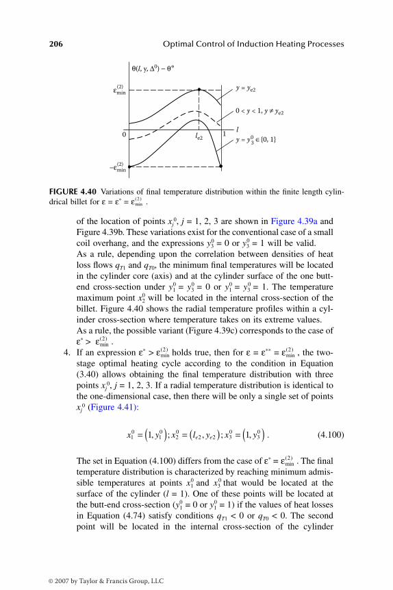
206 Optimal Control of Induction Heating Processes
of the location of points xj0, j = 1, 2, 3 are shown in Figure 4.39a and
Figure 4.39b. These variations exist for the conventional case of a smallcoil overhang, and the expressions y3
0 = 0 or y30 = 1 will be valid.
As a rule, depending upon the correlation between densities of heatloss flows qT1 and qT0, the minimum final temperatures will be locatedin the cylinder core (axis) and at the cylinder surface of the one butt-end cross-section under y1
0 = y30 = 0 or y1
0 = y30 = 1. The temperature
maximum point x20 will be located in the internal cross-section of the
billet. Figure 4.40 shows the radial temperature profiles within a cyl-inder cross-section where temperature takes on its extreme values.As a rule, the possible variant (Figure 4.39c) corresponds to the case ofε* > .
4. If an expression ε* > holds true, then for ε = ε** = , the two-stage optimal heating cycle according to the condition in Equation(3.40) allows obtaining the final temperature distribution with threepoints xj
0, j = 1, 2, 3. If a radial temperature distribution is identical tothe one-dimensional case, then there will be only a single set of pointsxj
0 (Figure 4.41):
. (4.100)
The set in Equation (4.100) differs from the case of ε* = . The finaltemperature distribution is characterized by reaching minimum admis-sible temperatures at points x1
0 and x30 that would be located at the
surface of the cylinder (l = 1). One of these points will be located atthe butt-end cross-section (y1
0 = 0 or y10 = 1) if the values of heat losses
in Equation (4.74) satisfy conditions qT1 < 0 or qT0 < 0. The secondpoint will be located in the internal cross-section of the cylinder
FIGURE 4.40 Variations of final temperature distribution within the finite length cylin-drical billet for ε = ε* = .
0 1l
le2
y = ye2
0 < y < 1, y ≠ ye2
y = y03 ∈0, 1
θ(l, y, ∆0 ) − θ∗
εmin(2)
−εmin(2)
εmin( )2
εmin( )2
εmin( )2 εmin
( )2
x y x l y x ye e10
10
20
2 2 30
301 1= ( ) = ( ) = ( ), ; , ; ,
εmin( )2
DK6039_C004.fm Page 206 Thursday, June 8, 2006 12:34 PM
© 2007 by Taylor & Francis Group, LLC
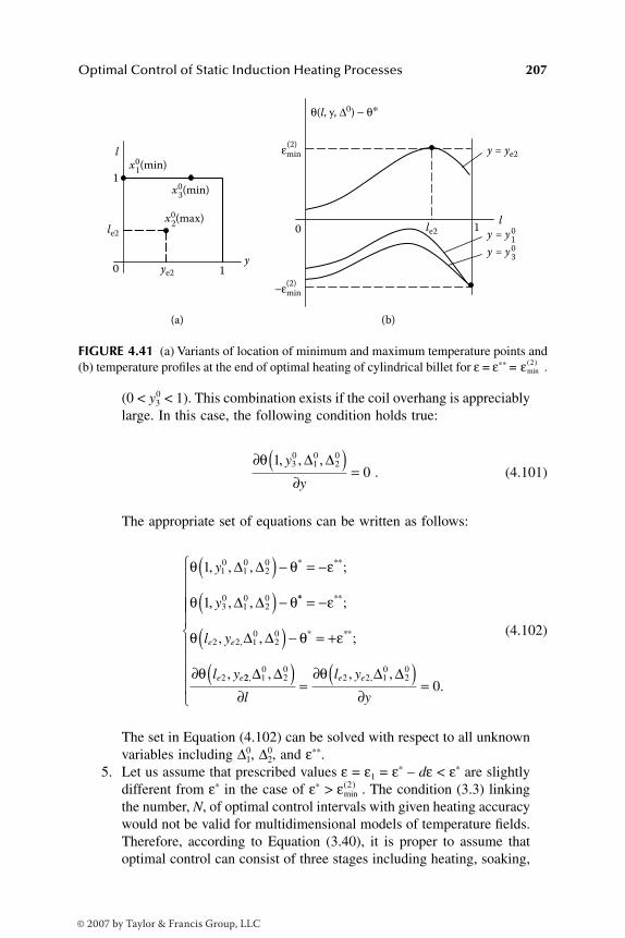
Optimal Control of Static Induction Heating Processes 207
(0 < y30 < 1). This combination exists if the coil overhang is appreciably
large. In this case, the following condition holds true:
. (4.101)
The appropriate set of equations can be written as follows:
(4.102)
The set in Equation (4.102) can be solved with respect to all unknownvariables including ∆1,
0 ∆2,0 and ε**.
5. Let us assume that prescribed values ε = ε1 = ε* – dε < ε* are slightlydifferent from ε* in the case of ε* > . The condition (3.3) linkingthe number, N, of optimal control intervals with given heating accuracywould not be valid for multidimensional models of temperature fields.Therefore, according to Equation (3.40), it is proper to assume thatoptimal control can consist of three stages including heating, soaking,
FIGURE 4.41 (a) Variants of location of minimum and maximum temperature points and(b) temperature profiles at the end of optimal heating of cylindrical billet for ε = ε** = .
l
le2le2
1
1
(a) (b)
10
0
y = ye2
θ(l, y, ∆0 ) − θ∗
εmin(2)
−εmin(2)
x02(max)
x01(min)
x03(min)
y = y01
y = y03
ye2
y
l
εmin( )2
∂ ( )∂
=θ 1
030
10
20, , ,y
y
∆ ∆
θ θ ε
θ θ
1
1
10
10
20
30
10
20
, , , ;
, , ,
* **y
y
∆ ∆
∆ ∆
( ) − = −
( ) − ** **
,* **
;
, , ;
,
= −
( ) − = +
∂
ε
θ θ ε
θ
l y
l y
e e
e e
2 2 10
20
2
∆ ∆
22 10
20
2 2 10
20
0, ,, , ,
.∆ ∆ ∆ ∆( )
∂=
∂ ( )∂
=
l
l y
y
e eθ
εmin( )2
DK6039_C004.fm Page 207 Thursday, June 8, 2006 12:34 PM
© 2007 by Taylor & Francis Group, LLC
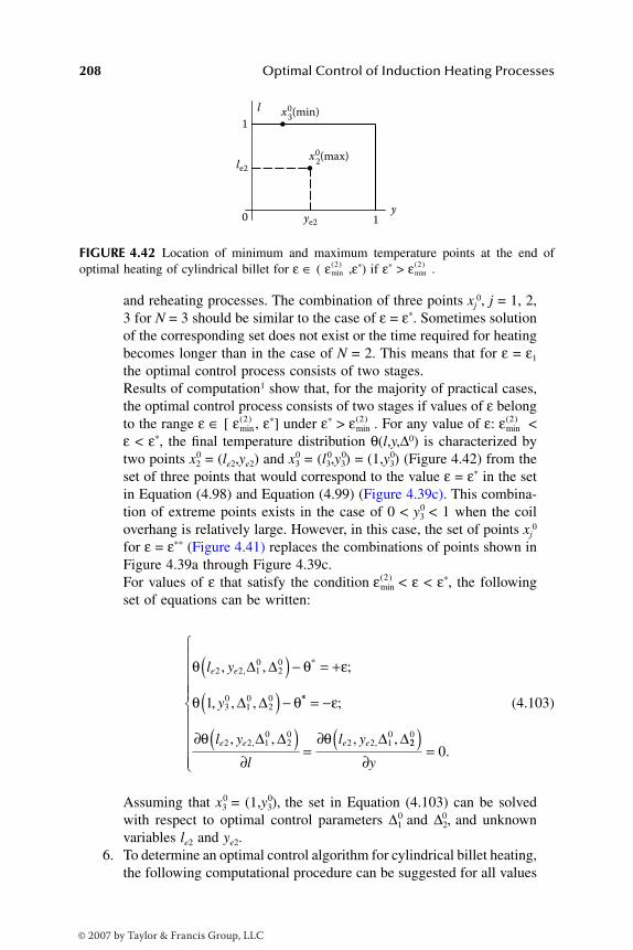
208 Optimal Control of Induction Heating Processes
and reheating processes. The combination of three points xj0, j = 1, 2,
3 for N = 3 should be similar to the case of ε = ε*. Sometimes solutionof the corresponding set does not exist or the time required for heatingbecomes longer than in the case of N = 2. This means that for ε = ε1
the optimal control process consists of two stages. Results of computation1 show that, for the majority of practical cases,the optimal control process consists of two stages if values of ε belongto the range ε ∈ [ , ε*] under ε* > . For any value of ε: <ε < ε*, the final temperature distribution θ(l,y,∆0) is characterized bytwo points x2
0 = (le2,ye2) and x30 = 0(l3,y3)
0 = (1,y3)0 (Figure 4.42) from the
set of three points that would correspond to the value ε = ε* in the setin Equation (4.98) and Equation (4.99) (Figure 4.39c). This combina-tion of extreme points exists in the case of 0 < y3
0 < 1 when the coiloverhang is relatively large. However, in this case, the set of points xj
0
for ε = ε** (Figure 4.41) replaces the combinations of points shown inFigure 4.39a through Figure 4.39c.For values of ε that satisfy the condition < ε < ε*, the followingset of equations can be written:
(4.103)
Assuming that x30 = (1,y3),
0 the set in Equation (4.103) can be solvedwith respect to optimal control parameters ∆1
0 and ∆2,0 and unknown
variables le2 and ye2.6. To determine an optimal control algorithm for cylindrical billet heating,
the following computational procedure can be suggested for all values
FIGURE 4.42 Location of minimum and maximum temperature points at the end ofoptimal heating of cylindrical billet for ε ∈ ( ,ε*) if ε* > .
l
le2
1
10
x02(max)
x03(min)
ye2
y
εmin( )2 εmin
( )2
εmin( )2 εmin
( )2 εmin( )2
εmin( )2
θ θ ε
θ θ
l y
y
e e2 2 10
20
30
10
201
, , ;
, , ,
,*∆ ∆
∆ ∆
( ) − = +
( ) − **
, ,
;
, , , ,
= −
∂ ( )∂
=∂
ε
θ θl y
l
l ye e e e2 2 10
20
2 2 10∆ ∆ ∆ ∆22
0
0( )
∂=
y
.
DK6039_C004.fm Page 208 Thursday, June 8, 2006 12:34 PM
© 2007 by Taylor & Francis Group, LLC
Optimal Control of Static Induction Heating Processes 209
of ε ∈ [ , ]. As value ε decreases from to , there mightbe one of two possible profiles of the final temperature distributiondepending upon distribution of heating power along the heater length.In the case of a relatively small coil overhang, the condition ε* = will be valid. The temperature distribution (Figure 4.38a and Figure4.38b) can be changed as shown in Figure 4.39a and Figure 4.39b. Theappropriate set of equations (Equation 4.98 and Equation 4.99) ought tobe solved instead of the set in Equation (4.96) through Equation (4.98).If the coil overhang is large enough, then the inequality ε* > holdstrue. This case is represented by the sequential variations of tempera-ture distribution in Figure 4.38c, Figure 4.39c, Figure 4.42, and Figure4.41a. The appropriate sets of equations in Equation (4.96), Equation(4.98), Equation (4.99), Equation (4.103), and Equation (4.102) canbe written. Particular scenarios could be revealed by solving a sequenceof optimal control problems for the series of fixed values ε descendingby sufficiently small steps from initial value to value . If ε =ε0 and given value ε0 ∈ [ , ], then solution of the initial optimalcontrol problem can be found during the appropriate step of thedescribed computation procedure.
7. The preceding provided analysis proves that optimal control parametersdepend on coil overhang h. Given expressions for Wd(ξ,l,y) in Equation(4.72) include function Wd
*(ξ,l,y,h), which describes a longitudinaldistribution of electromagnetic heat sources as function of coil over-hang h. The temperature field θ(l,y,∆,h) in the form of Equation (4.94)or Equation (4.95) can be considered as a function of h (becausecoefficients Wrn, r, n = 0, 1, 2, … depend on h). Therefore, the variableh can be considered as one of the unknown parameters of the optimalprocess. Solution of the optimal control problem allows finding thevector of optimal control parameters ∆0 and the value of coil overhangh* that corresponds to the best heating accuracy attainable undertwo-stage control:
. (4.104)
As the number of unknown parameters is increased by one, thenaccording to Equation (3.39) and Equation (3.40), the number of pointsxj
0 increases at least by one in contrast to the case when values of hdiffer from value h*.In the case of ε = , two possible sets of extreme points xj
0 exist:for = ε* (Figure 4.39a and Figure 4.39b) and for = ε** (Figure4.41). The combination of these sets corresponds to the case of h = h*
(Figure 4.43).Instead of Equation (4.102), the following set of equations can be
written with respect to four points 0xJ, j = :
εmin( )2 εmin
( )1 εmin( )1 εmin
( )2
εmin( )2
εmin( )2
εmin( )1 εmin
( )2
εmin( )2 εmin
( )1
εminmin( )2
ε εminmin minmin2 2( ) ( )= ( )h
h
εmin( )2
εmin( )2 εmin
( )2
1 4,
DK6039_C004.fm Page 209 Thursday, June 8, 2006 12:34 PM
© 2007 by Taylor & Francis Group, LLC

210 Optimal Control of Induction Heating Processes
(4.105)
The minimum admissible temperature is reached at three points.The set in Equation (4.105) can be solved with respect to six unknownvariables: the value of optimal coil overhang h*, “global” minimax
and optimal control parameters ∆1,0 ∆2,
0 le2, and ye2. It is possibleto show that condition = ε* is valid under h < h* and the expression
= ε** is true under h > h*. In both cases, the condition> holds true for all values h ≠ h*.
8. In the case of ε0 < , the optimal control problem should be solvedusing the computational technique described in Section 3.7. Usingadditional information with respect to temperature distribution that isbased on physical nature of induction heating processes, it is possibleto further simplify the computation process by applying analogies withthe conventional case of ε0 < for the one-dimensional problem.
FIGURE 4.43 Location of minimum and maximum temperature points within cylindricalbillet for value of coil overhang that corresponds to the best heating accuracy under two-stage optimal control.
l
le2
1
10
x02(max)
x01(max)
x03(min)
x04(min)
ye2
y
θ θ ε
θ
0 10
10
20 2
2 2
, , , , ;
,
* *minminy h
l ye e
∆ ∆( ) − = − ( )
,,* *
minmin, , ;
, , ,
∆ ∆
∆ ∆
10
20 2
30
10
201
h
y
( ) − = ( )θ ε
θ ,, ;
, , , ,
* *minmin
*
h
y h
( ) − = −
( ) −
( )θ ε
θ θ
2
40
10
201 ∆ ∆ **
minmin
,*
;
, , ,
= −
∂ ( )∂
=∂
( )ε
θ θ
2
2 2 10
20l y h
l
le e ∆ ∆ ee ey h
y
2 2 10
20
0, , ,
.,
*∆ ∆( )∂
=
εminmin( )2
εmin( )2
εmin( )2
εmin( )2 εminmin
( )2
εmin( )2
εmin( )2
DK6039_C004.fm Page 210 Thursday, June 8, 2006 12:34 PM
© 2007 by Taylor & Francis Group, LLC

Optimal Control of Static Induction Heating Processes 211
In the practicable cases the optimal control process consists of one, two, orthree stages, and the condition in Equation (3.3) directly links the number ofcontrol stages with preset value of ε.1 Table 4.1 shows some results of computationof optimal cylindrical billets heating for the initial data: ξ = 4; β = 0.214; θ* =0; Umax = 1. Similarly to the one-dimensional model, heat source distributionalong the billet length is assumed to be uniform.1 Initial and boundary conditions(Equation 4.73 and Equation 4.75) are considered under the following assump-tion:
θ0(l,y) = θa(ϕ) = θal(ϕ) = θa0(ϕ) θ0 = –0.5 = const.
This case corresponds to the condition ε* = .Computation results (Table 4.1) show that, due to considering heat losses
from billet butt-ends, the heating accuracy decreases in comparison with the one-dimensional problem. The last line of Table 4.1 shows results for one-dimensionalOCP solution (assuming that butt-end heat losses are neglected Bi0 = Bi1 = 0).More complicated problems of time-optimal control can be solved using thecomputational technique described in Section 4.1 through Section 4.3. Similarlyto the one-dimensional case (Section 4.1), the final temperature distribution isnot changed if technological restraints are taken into account.
Control input functions uσ and uθ can be found similarly to the techniquedescribed in Section 4.1.2. Instead of Expression (4.9) and Expression (4.13),they can be approximated as weighted sum of the constant component and twoexponential summands.1 In the case of ε ≥ = εinf and αT < 1 in Equation(4.30), the governing set of equations remains unchanged. This conclusion isbased on analogies with the one-dimensional time-optimal problem subject tothe transfer stage (Section 4.2).
Similarly to Equation (4.41) and Equation (4.42) for the conventional caseof ε = = εinf (assuming αT = 1 in Equation 4.30), it is possible to obtain thefollowing set of equations:
(4.106)
The first equation of the set in Equation (4.106) is written with respect tominimum temperature at the point (1,y1)
0 on the cylinder lateral surface under le2
≥ 0 (Figure 4.42). The set in (Equation 4.106) can be solved using additionalinformation with respect to the axial coordinate of the temperature minimum
εmin( )2
εmin( )2
εmin( )2
θ θ ε
θ
T T
e e
y
l y
1 10
10 0 2
2 2 10
, , , ;
, ,
*min∆ ∆
∆
( ) − = − ( )
,, ;
, ,
*min
,
∆
∆ ∆
T
T e e Tl y
l
0 2
2 2 10 0
( ) − = +
∂ ( )∂
( )θ ε
θ
==∂ ( )
∂=
θT e e Tl y
y
2 2 10 0
0, ,
.,∆ ∆
DK6039_C004.fm Page 211 Thursday, June 8, 2006 12:34 PM
© 2007 by Taylor & Francis Group, LLC

212O
ptim
al Co
ntro
l of In
du
ction
Heatin
g Processes
TABLE 4.1Optimal Process Parameters for Heating of Cylindrical Billet
N = 1 N = 2
Bi Bi0 Bi1 0y1 ye2 le2 ∆∆∆∆10 εεεεmin
(1) 0y10y3 ye2 le2 ∆∆∆∆1
0 ∆∆∆∆20 ϕϕϕϕmin
0 εεεεmin(2)
0.7 1.4 1.4 0 0.5 0.860 0.364 0.095 0 0.5 0.647 0.372 0.0421 0.4141 0.04840.7 0.7 0.7 0 0.5 0.861 0.356 0.086 0 0.5 0.650 0.361 0.0423 0.4033 0.03600.7 0 0 — — 0.889 0.347 0.077 — — 0.661 0.349 0.0426 0.3916 0.0237
DK
6039_C004.fm
Page 212 Thursday, June 8, 2006 12:34 PM
© 2007 by Taylor &
Francis Group, LLC

Optimal Control of Static Induction Heating Processes 213
point 0y1. Similarly to Equation (4.105), it is possible to obtain the system ofequations that corresponds to coil overhang value h = h* in the time-optimalcontrol problem, taking into consideration the transfer stage.
In this case, additional point x30 (compare with Equation 4.106) appears
because the minimum temperature can be reached at one of two points on thecylinder lateral surface: in the internal cross-section (0 < y1
0 < 1) or in the butt-end cross-section (y1
0 = 0 or y10 = 1). These variations of location of temperature
minimum will be similar to the variant shown in Figure 4.41. The combinationof both scenarios allows obtaining the following set of equations:
(4.107)
where y10 = 0 or y1
0 = 1; 0 < y30 < 1. Expression for θT(l,y,∆1,∆T)
0 can be foundsimilarly to Equation (4.34) through Equation (4.36). This expression will includefourfold series instead of twofold series in Equation (4.34).
The technique described in Section 4.3 allows taking into account incompleteinformation with respect to the heating system under control. In real-life produc-tion situations, we often face incompleteness of source information with respectto the induction heating system. Incompleteness of information is caused, firstof all, by imperfection of our knowledge about certain features of the heatingsystem. This includes but is not limited to uncertainties of electromagnetic andthermal-physical properties of heated billets, inductor geometry, power supplylimitations, presence of harmonics, etc.
On another hand, there are uncertainties with respect to particular conditionsof the technological process. Initial temperature distribution of the heated work-piece and/or the value of heat losses from its surface to the surrounding areacould be regarded as other examples of incompletely defined operating charac-teristics of the heating process (Section 4.3). It is assumed that these disturbancescan be taken into account while solving optimal-control problems. For this pur-pose, each equation of the governing set should be considered for appropriateparticular values of ill-defined characteristics. These values should be chosenwithin possible variation intervals.
Let us consider as an example a two-dimensional problem of time-optimalcontrol of induction heating of aluminum alloy cylindrical billets.1 Figure 4.44represents some results of computation for ε = .
θ θ ε
θ
T T
T
y h
y
1
1
10
10 0 2
3
, , , , ;
,
* *minmin∆ ∆( ) − = − ( )
0010 0 2
2 2
, , , ;
, ,
* *minmin∆ ∆
∆
T
T e e
h
l y
( ) − = − ( )θ ε
θ
110 0 2
2 2 10
, , ;
,
* *minmin
,
∆
∆
T
T e e
h
l y
( ) − = +
∂
( )θ ε
θ
,, , , , ,,
*,
*∆ ∆ ∆T T e e Th
l
l y h
y
02 2 1
0 0
0( )
∂=
∂ ( )∂
=
θ
εmin( )2
DK6039_C004.fm Page 213 Thursday, June 8, 2006 12:34 PM
© 2007 by Taylor & Francis Group, LLC

214 Optimal Control of Induction Heating Processes
Calculations were performed taking into account constraint on maximumtemperature and constraint imposed on transportation time. Incomplete informationwith respect to initial temperature and level of heat losses (during heating andtransfer stages) has been considered in order to have a proper OCP formulation.Similarly to the one-dimensional problem, it was assumed that distribution of heatsource power could be considered as uniform along the billet length.
Computations of the optimal process have been conducted with respect toconstant surface heat losses that can be estimated by relative values Bih (duringthe heating stage) and BiT (during the transfer stage). The preset value ∆T =
0∆T
should satisfy the condition ∆T0 < ∆T2
* and, therefore, the inequality αT < 1 remainsvalid. Under incomplete information with respect to parameters θ0, Bih , and BiT,it is assumed that the maximum temperature is reached for Bih = Bihmin, BiT =BiTmin, and θ0 = θ0max; minimum temperature is reached for Bih = Bihmax, BiT =BiTmax, and θ0 = θ0min.
In the case of ε = , αT < 1 computational sets keep the form of Equation(4.98), Equation (4.99) or Equation (4.102) with substitution θT( )instead of θ( ). The function θT( ) can be calcu-
FIGURE 4.44 Optimal control, time–temperature history, and final temperature profilesin the two-dimensional problem of time-optimal control for induction heating of D19aluminum alloy cylindrical billets (diameter is 240 mm; length is 835 mm; requiredtemperature is 400°C). Γ = 1; θ0 ∈ [–0.50;–0.44]; Bih ∈ [0.015;0.050]; BiT ∈ [0.10;0.12];ξ = 20; θadm = 0.09; θ* = 0; ∆T
0 = 50 s; ε0 = ; h = 1.75 mm. 1: optimal control uθ(ϕ)= Umax 0.24 + 0.264 exp[–8.3(ϕ – ϕθ)] + 0.002 exp[–4.4(ϕ – ϕθ)]; 2: temperature atpoint l = 1; y = 0.5; under θ0 = –0.44; Bih = 0.015; BiT = 0.10; 3: temperature at point l= 1; y = 0; under θ0 = –0.5; Bih = 0.05; BiT = 0.12; 4: temperature at point l = 0; y = 0;under θ0 = –0.5; Bih = 0.05; BiT = 0.12; 5: final temperature profile at y = 0.5; under θ0 =–0.44; Bih = 0.015; BiT = 0.10; 6: final temperature profile at y = 0; θ0 = –0.5; under Bih
= 0.050; BiT = 0.12.
Δ01
Δ0T
Δ02
1 2
3
uθ
4
0 200 400 600 1000 1200 τ, s
ϕθ
200
100
80
160
240
320
400
m2
kW P,
800
5
6
0
40
−40
1 l
t,°C
t − t∗, °C
Umax
εmin( )2
εmin( )2
l yj j T0 0
10
20 0, , , ,∆ ∆ ∆
l yj j T0 0
10
20 0, , , ,∆ ∆ ∆ l yj j T
0 010
20 0, , , ,∆ ∆ ∆
DK6039_C004.fm Page 214 Thursday, June 8, 2006 12:34 PM
© 2007 by Taylor & Francis Group, LLC

Optimal Control of Static Induction Heating Processes 215
lated at each of points (lj0,yj
0) for the set of values 0(Bihj,BiTj,θ0j)0 chosen0 in the
same manner. Figure 4.44 shows that, similarly to Figure 4.39a (or Figure 4.39b),the final temperature distribution is characterized by combination of points xj
0.In this case, it is possible to obtain = ε* = 40°C. According to denotations
discussed in Section 4.2 and Section 4.3, the upper indexes “~” and “–“ indicatethat solution of the optimal control problem has been found in the class of two-stage control, taking into account the condition ∆T ≠ 0 and uncertainty in thedefinition of values Bi, BiT, and θ0. The optimal power control algorithm can bewritten in the form of Expression (4.3) for N = 2. In contrast to the case ofEquation (4.9), the control input uθ(ϕ) can be described by the sum of twoexponential summands.
4.5.4 TIME-OPTIMAL CONTROL OF INDUCTION HEATING OF RECTANGULAR-SHAPED WORKPIECES
Slabs, plates, and blooms of various shapes and thicknesses may be heated andlater rolled down to the final desired size. Some of these are cooled and laterreheated for rolling or forming; others are reheated as a part of the continuousprocess to facilitate the subsequent rolling or forming operation.1 This section isdevoted to discussion of optimal induction heating of rectangular-shaped work-pieces.
Solution of the two-dimensional time-optimal control problem for heating ofrectangular-shaped workpieces is noticeably different compared to previouslydescribed cases. The condition Γ = 0 should be accepted in Equation (4.72)through Equation (4.75). In this case, direct analogies with one-dimensionalmodels cannot be applied.16,17 The two-dimensional mathematical model (Equa-tion 4.72 through Equation 4.75) describes temperature distribution in the planeof the cross-section of rectangular-shaped workpieces, assuming uniform tem-perature distribution along the workpiece length.
This means that inductor load can be approximately considered as a rectan-gular prism of infinite length (Figure 4.37). Similarly to the problem for heatingof finite length cylindrical billets, the time-optimal control problem can bereduced to the form of Equation (4.93). The complicated shape of final temper-ature distribution in the slab cross-section adds complexity to the solution of OCP.
4.5.4.1 Surface Heat-Generating Sources
Internally generated heating power is the most significant process parameter thataffects temperature distribution (Section 2.4). Proper control of the heating pro-cess involves appropriate choice of induced power density. Complication of thecontrol process occurs due to difficulties in providing desired spatial distributionof internal heat sources. It could be impractical to realize certain power distribu-tion along the length of the induction coil. Many of the existing means to controlpower distribution face strict limitations or merely cannot produce a particularspatial distribution of internal heat sources when heating certain metals.
εmin( )2
DK6039_C004.fm Page 215 Thursday, June 8, 2006 12:34 PM
© 2007 by Taylor & Francis Group, LLC
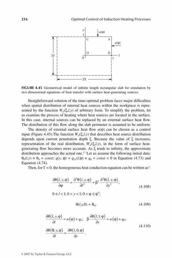
216 Optimal Control of Induction Heating Processes
Straightforward solution of the time-optimal problem faces major difficultieswhen spatial distribution of internal heat sources within the workpiece is repre-sented by the function Wd(ξ,l,y) of arbitrary form. To simplify the problem, letus examine the process of heating where heat sources are located in the surface.In this case, internal sources can be replaced by an external surface heat flow.The distribution of this flow along the slab perimeter is assumed to be uniform.
The density of external surface heat flow u(ϕ) can be chosen as a controlinput (Figure 4.45).The function Wd(ξ,l,y) that describes heat source distributiondepends upon current penetration depth ξ. Because the value of ξ increases,representation of the real distribution, Wd(ξ,l,y), in the form of surface heat-generating flow becomes more accurate. As ξ tends to infinity, the approximatedistribution approaches the actual one.17 Let us assume the following initial data:θ0(l,y) ≡ θ0 = const; q(y, ϕ) = qT1(l,ϕ) ≡ q0 = const < 0 in Equation (4.73) andEquation (4.74).
Then, for Γ = 0, the homogeneous heat conduction equation can be written as1:
(4.108)
θ(l,y,0) = θ0; (4.109)
(4.110)
FIGURE 4.45 Geometrical model of infinite length rectangular slab for simulation bytwo-dimensional equations of heat transfer with surface heat-generating sources.
0 1l
2X
1
y u(ϕ)
u(ϕ)
2YO
C A
D
∂ ( )∂
=∂ ( )
∂+
∂ ( )∂
θ ϕϕ
θ ϕβ
θ ϕl y l y
l
l y
y
, , , , , ,;
2
22
2
2
0 << < < < < ≤l y1 0 1 0 0; ; ;ϕ ϕ
∂ ( )∂
= ( ) + ∂ ( )∂
= ( ) +
∂
θ ϕϕ β
θ ϕϕ
θ
1 10 0
, ,;
, ,;
y
lu q
l
yu q
00 0, , , ,.
y
l
l
y
ϕ θ ϕ( )∂
=∂ ( )
∂
DK6039_C004.fm Page 216 Thursday, June 8, 2006 12:34 PM
© 2007 by Taylor & Francis Group, LLC

Optimal Control of Static Induction Heating Processes 217
The control input u(ϕ) is included into the boundary conditions (Equation 4.110).The optimal control by density of heat flow from the surface has the same
form of Equation (2.27) as the control by density of internal heat sources. Thecontrol function is constrained by the condition in Equation (2.7).
According to the boundary condition (Equation 4.110), the optimal heatingprocess consists of alternating stages of heating with heat flow density Umax + q0
< Umax and subsequent soaking under heat losses q0 < 0. In all practicable casesit can be assumed that |q0| < Umax and Umax + q0 > 0. The number, N ≥ 1, of stagescan be uniquely defined based on given heating accuracy ε and it increases withdecrease of ε. Therefore, the shape of the optimal control algorithm is known,but the number of stages, N, and durations, ∆1, ∆2, …, ∆N, of those stages remainunknown.
The expression for temperature field θ(l,y,∆) can be obtained in the explicitform as a function of spatial coordinates and optimal control parameters ∆i, i= 1:
(4.111)
The optimal control problem is reduced to searching for number, N, andoptimal values of parameters 0∆i, i = that uniquely specify the optimalcontrol input.
1 N,
θ θ βl y qU m
m
, , max∆( ) = + +( ) + + −( )( )
+0 0
11
21 1
==
+
∑ − −
×
× + + −( )( )
1
2
01
12
13
21 1
N
m
N
l
qU
∆
max
− −
+ + −( )( )
+12
13 2
1 120
1
βy q
U Nmax +
+ −( ) ⋅ +( ) −+
=
∞
=∑2 1
1
1
02 2
1
r
r
m
m
N
U q rmax exp π ∆∑∑ ∑
+ −( )
×
× −
+
=
=
U
r
j
j
N
m
m
max
exp
11
2
2 2π ∆jj
Nn
n
rl
r∑ ∑
+ −( ) ×
×
+
=
∞cos ππ β2 2
1
1
21
UU q n Um
m
Nj
max maxexp+( ) −
+ −( )
=∑0
2 2 2
1
1π β ∆ ++
=
=
∑
∑
×
× −
1
2
2 2 2
j
N
m
m j
N
nexp π β ∆ ccos.
ππ
ny
n2 2
1 N,
DK6039_C004.fm Page 217 Thursday, June 8, 2006 12:34 PM
© 2007 by Taylor & Francis Group, LLC

218 Optimal Control of Induction Heating Processes
Problems of this type can be solved for the conventional case of ε ∈[ , ].1,18,19
Optimal single-stage control. In the simplest case of ε = similar to heatingof the cylindrical billet (Section 4.5.3), one can assume that N = 1. Undermaximum heat flow from the slab surface, the maximum and minimum finaltemperatures can be reached only at two points x1
0 = (0,0) and x20 = (1,1), respec-
tively: in the vertices O(l = 0, y = 0) and A(l = 1, y = 1) of rectangular cross-section OCAD (Figure 4.46a). With regard to Equation (3.39) and Equation (3.40)for ε = under R = N + 1 = 2, at the end of the time-optimal process, maximumdeviations of final temperature from the required one, θ*, will be reached at thesepoints with different signs. As a result, the basic system of correlations (Equation3.39) can be transformed into the appropriate set of two equations:
(4.112)
FIGURE 4.46 Variants of location of minimum and maximum temperature points withinrectangular slab cross-section at the end of single-stage and two-stage optimal control bypower of surface heat-generating sources for ε ∈ [ , ].
y1
0 1 1 1
O(min)
(a) (b)
(d) (e)
(c)
Cy
ye2
le2
le2 le2
le2
1
0
y
ye2
1
0 1
y
ye2
1
0 1
y
ye2
1
0
O(min) DP
C C(min)
C(min) C(min)
A
V
Ly
Ll
B(max)
B(max)
B(max)
M A
A
N
ε = εmin
(1) ε = ε1
(2)ε = ε′
Dl
O ODl
B(max)
A(min)
Dl
lO(min) D
l
A(max)
εmin
< ε < ε1
(2) (2) ε = ε2 = ε
min
(2) (2)
εmin( )2 εmin
( )1
εmin( )3 εmin
( )1
εmin( )1
εmin( )1
θ θ ε
θ θ ε
1 1
0 0
10 1
10 1
, , ;
, ,
*min
*min
∆
∆
( ) − =
( ) − = −
( )
( ))
.
DK6039_C004.fm Page 218 Thursday, June 8, 2006 12:34 PM
© 2007 by Taylor & Francis Group, LLC

Optimal Control of Static Induction Heating Processes 219
The set in Equation (4.112) can be solved with respect to two unknownvariables, ∆1
0 and , by substituting the expression for temperature field θ(l,y,∆)in the form of Equation (4.111).
Optimal two-stage control. Let us consider the case of ε = ε′ = – dε,where dε > 0 is a sufficiently small value. The continuous nature of the finaltemperature distribution θ(l,y,∆0) as a function of ε and inequality N ≥ 2 for ε′< allows establishing the following property of optimal final temperatureprofile θ(l,y,∆0(ε′)). The number, R, of points xj
0 in Equation (3.39) and Equation(3.40), where the maximum admissible absolute deviations of final temperatureare reached, is equal to number, N, of optimal control intervals, i.e., R = N = 2under ε = ε′.
Therefore, in the case of ε = ε′, the time-optimal control consists of twostages; at the end of heating, maximum admissible deviations are reached at twopoints: x1
0 = 0(l1,y1)0 and x2
0 = 0(l2,y2).0 This conclusion remains valid for all values
of ε decreasing from until, for some value ε = ε(2),1 the third point, x3,0 with
maximum temperature deviation appears in the prism cross-section. Accordingto the condition in Equation (3.40), three points xj
0 always exist for the value ε= ; therefore, the condition ε1
(2) ≥ will be valid. A similar situation hasbeen observed earlier when considering optimal heating of cylindrical billets(Section 4.5.3).
Variations of locations of points xj0, j = 1, 2, 3 could be set from the study
of final temperature distribution θ(l,y,∆) under two-stage control. The shape oftemperature field θ(l,y,∆0) can be uniquely determined by values of temperaturegradients, ∂θ(l,y,∆1,∆2)/∂l, ∂θ(l,y,∆1,∆2)/∂y, within the cross-section of the prism.
When passing from the first control stage under u(ϕ) ≡ Umax + q0 > 0 to thesecond one under u(ϕ) ≡ q0 < 0, the temperature gradients on the border of thecross-section (on the lines l = 1 and y = 1) change their signs. This means thatonly two lines, Ll and Ly , appear in the plane of rectangle OCAD, for which thefollowing conditions remain valid: ∂θ(l,y,∆1,∆2)/∂l = 0 and ∂θ(l,y,∆1,∆2)/∂y = 0,respectively (Figure 4.46).
It is important to underline that these conditions remain valid for the pointsthat belong to the rectangle’s sides y = 0 and l = 0. There is a general analogyto the previously described one-dimensional case where not more than one extre-mum point (i.e., the point with zero gradient) appears if the number of controlstages increases by one (Section 3.2). As it follows from Equation (4.111), theexpression for final temperature distribution can be represented as a sum, andeach summand depends only on one of the spatial coordinates:
, (4.113)
where β2∆ = (β2∆1, β2∆2, …, β2∆N).With regard to the control input (Equation 2.27) applied on borders l = 1 and
y = 1, functions θ1(l,∆) and θ2(y,β2∆) (in relative units) describe one-dimensional
εmin( )1
εmin( )1
εmin( )1
εmin( )1
εmin( )2 εmin
( )2
θ θβ
θ βl y l y, , , ,∆ ∆ ∆( ) = ( ) + ( )1 221
DK6039_C004.fm Page 219 Thursday, June 8, 2006 12:34 PM
© 2007 by Taylor & Francis Group, LLC

220 Optimal Control of Induction Heating Processes
temperature fields within infinitely long plates of thickness 2X and 2Y, respec-tively.
According to Equation (4.113), the following conditions are met:
(4.114)
This implies that lines Ll and Ly represents straight lines in the plane of therectangular cross-section of the prism. They are parallel to coordinate axes y andl, respectively (Figure 4.46b through Figure 4.46e). During the first controlinterval under maximum heating power, the temperature gradients ∂θ/∂l and ∂θ/∂yare positive within the whole prism cross-section — i.e., at any point of rectangleOCAD.
When passing on to the second interval, straight lines Ll and Ly of zero gradientappear on borders l = 1 and y = 1 and then they move towards coordinate axesl = 0 and y = 0 (Figure 4.46b through Figure 4.46e), leaving behind the negativegradients zone adjoining surfaces l = 1 and y = 1. If only one straight line, Ll, aswell as only one line, Ly , exists in the plane of rectangle OCAD, then signs ofgradients will be the same except on these lines. Therefore, gradients remainpositive in the areas prior to these lines in the same way as during the first controlinterval. As a result, straight lines Ll and Ly divide rectangle OCAD into regionsof positive and negative gradients. This allows determining their signs at anypoint of this rectangle in the end of ∂θ/∂l two-stage optimal control process(Figure 4.46b).
For the second interval, the following conditions can be obtained:
(4.115)
According to boundary conditions in Equation (4.110), the temperature gra-dient will be equal to zero only on the lines Ll and Ly and on the sides l = 0 andy = 0.
∂ ( )∂
=∂ ( )
∂∈[ ]
∂
θ θ
θ
l y
l
l
lfor all y
l y
, , ,, ;
, ,
∆ ∆
∆
1 0 1
(( )∂
=∂ ( )
∂∈[ ]
y
y
yfor all l
10 1
22
βθ β,
, .∆
∂ ( )∂
≥
∂ ( )∂
θ
θ
l y
l
l y
, ,
, ,
∆
∆
0 for rectangle OCMP;
yy
l y
l
≥
∂ ( )∂
≤
0
0
for rectangle OVND;
for rθ , , ∆
eectangle PMAD;
for rectangle ∂ ( )
∂≤
θ l y
y
, , ∆0 VVCAN.
DK6039_C004.fm Page 220 Thursday, June 8, 2006 12:34 PM
© 2007 by Taylor & Francis Group, LLC
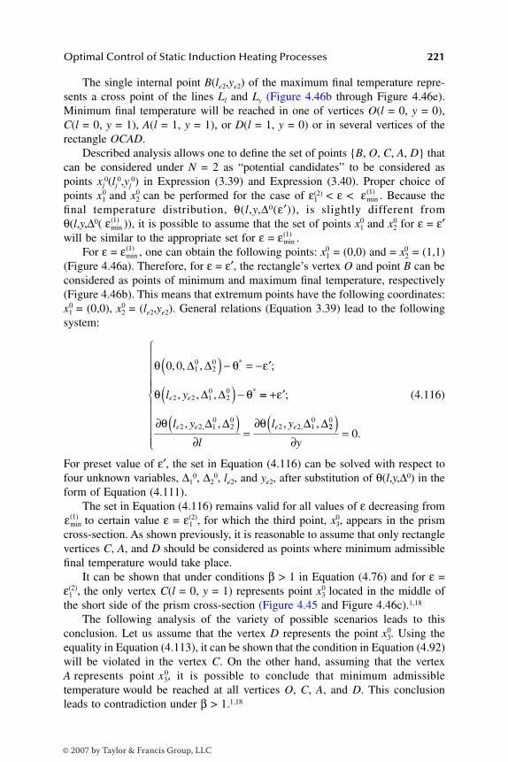
Optimal Control of Static Induction Heating Processes 221
The single internal point B(le2,ye2) of the maximum final temperature repre-sents a cross point of the lines Ll and Ly (Figure 4.46b through Figure 4.46e).Minimum final temperature will be reached in one of vertices O(l = 0, y = 0),C(l = 0, y = 1), A(l = 1, y = 1), or D(l = 1, y = 0) or in several vertices of therectangle OCAD.
Described analysis allows one to define the set of points B, O, C, A, D thatcan be considered under N = 2 as “potential candidates” to be considered aspoints xj
0(lj0,yj
0) in Expression (3.39) and Expression (3.40). Proper choice ofpoints x1
0 and x20 can be performed for the case of ε1
(2) < ε < . Because thefinal temperature distribution, θ(l,y,∆0(ε′)), is slightly different fromθ(l,y,∆0( )), it is possible to assume that the set of points x1
0 and x20 for ε = ε′
will be similar to the appropriate set for ε = .For ε = , one can obtain the following points: x1
0 = (0,0) and = x20 = (1,1)
(Figure 4.46a). Therefore, for ε = ε′, the rectangle’s vertex O and point B can beconsidered as points of minimum and maximum final temperature, respectively(Figure 4.46b). This means that extremum points have the following coordinates:x1
0 = (0,0), x20 = (le2,ye2). General relations (Equation 3.39) lead to the following
system:
(4.116)
For preset value of ε′, the set in Equation (4.116) can be solved with respect tofour unknown variables, ∆1
0, ∆20, le2, and ye2, after substitution of θ(l,y,∆0) in the
form of Equation (4.111).The set in Equation (4.116) remains valid for all values of ε decreasing fromto certain value ε = ε(2),1 for which the third point, x3,
0 appears in the prismcross-section. As shown previously, it is reasonable to assume that only rectanglevertices C, A, and D should be considered as points where minimum admissiblefinal temperature would take place.
It can be shown that under conditions β > 1 in Equation (4.76) and for ε =ε(2),1 the only vertex C(l = 0, y = 1) represents point x3
0 located in the middle ofthe short side of the prism cross-section (Figure 4.45 and Figure 4.46c).1,18
The following analysis of the variety of possible scenarios leads to thisconclusion. Let us assume that the vertex D represents the point 0x3. Using theequality in Equation (4.113), it can be shown that the condition in Equation (4.92)will be violated in the vertex C. On the other hand, assuming that the vertexA represents point 0x3, it is possible to conclude that minimum admissibletemperature would be reached at all vertices O, C, A, and D. This conclusionleads to contradiction under β > 1.1,18
εmin( )1
εmin( )1
εmin( )1
εmin( )1
θ θ ε
θ θ
0 0 10
20
2 2 10
20
, , , ;
, , ,
*
*
∆ ∆
∆ ∆
( ) − = − ′
( ) −l ye e == + ′
∂ ( )∂
=∂
ε
θ θ
;
, , , ,, ,l y
l
l ye e e e2 2 10
20
2 2 10∆ ∆ ∆ ∆22
0
0( )
∂=
y
.
εmin( )1
DK6039_C004.fm Page 221 Thursday, June 8, 2006 12:34 PM
© 2007 by Taylor & Francis Group, LLC
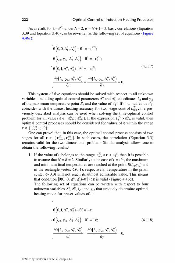
222 Optimal Control of Induction Heating Processes
As a result, for ε = ε1(2) under N = 2, R = N + 1 = 3, basic correlations (Equation
3.39 and Equation 3.40) can be rewritten as the following set of equations (Figure4.46c):
(4.117)
This system of five equations should be solved with respect to all unknownvariables, including optimal control parameters ∆1
0 and ∆2,0 coordinates le2 and ye2
of the maximum temperature point B, and the value of 1ε(2). If obtained value 1ε(2)
coincides with the utmost heating accuracy for two-stage control , the pre-viously described analysis can be used when solving the time-optimal controlproblem for all values ε ∈ [ , ]. If the expression 1ε(2) > is valid, thenoptimal control processes should be considered for values of ε within the rangeε ∈ [ ,ε1
(2)].One can prove1 that, in this case, the optimal control process consists of two
stages for all ε ∈ [ , ]. In such cases, the correlation (Equation 3.3)remains valid for the two-dimensional problem. Similar analysis allows one toobtain the following results.1
1. If the value of ε belongs to the range < ε < 1ε(2), then it is possibleto assume that N = R = 2. Similarly to the case of ε = 1ε(2), the maximumand minimum final temperatures are reached at the point B(le2,ye2) andin the rectangle vertex C(0,1), respectively. Temperature in the prismcenter O(0,0) will not reach its utmost admissible value. This meansthat condition |θ(0, 0, 0∆1, 0∆2)–θ*| < ε is valid (Figure 4.46d).The following set of equations can be written with respect to fourunknown variables 0∆1, ∆2,
0 le2, and ye2 that uniquely determine optimalheating mode for preset values of ε:
(4.118)
θ θ ε
θ
0 0 10
20
12
2 2 10
20
, , , ;
, , ,
*∆ ∆
∆ ∆
( ) − = −
( )
( )
l ye e −− = +
( ) − = −
∂
θ ε
θ θ ε
θ
* ( )
* ( )
;
, , , ;
,
12
10
20
12
2
0 1 ∆ ∆
le yy
l
l y
y
e e e2 10
20
2 2 10
20
0, ,, , ,
.∆ ∆ ∆ ∆( )
∂=
∂ ( )∂
=
θ
εmin( )2
εmin( )2 εmin
( )1 εmin( )2
εmin( )2
εmin( )2 εmin
( )1
εmin( )2
θ θ ε
θ θ
0 1 10
20
2 2 10
20
, , , ;
, , ,
*
*
∆ ∆
∆ ∆
( ) − = −
( ) − =l ye e ++
∂ ( )∂
=∂
ε
θ θ
;
, , , ,, ,l y
l
l ye e e e2 2 10
20
2 2 10
20∆ ∆ ∆ ∆(( )
∂=
y
0.
DK6039_C004.fm Page 222 Thursday, June 8, 2006 12:34 PM
© 2007 by Taylor & Francis Group, LLC
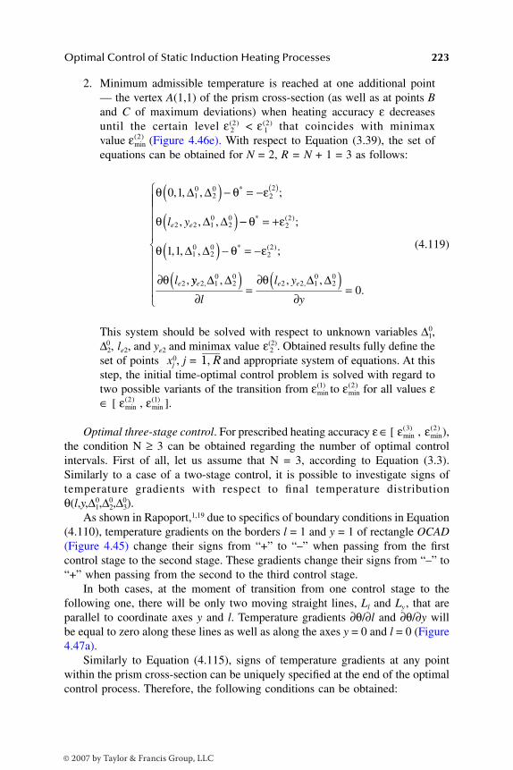
Optimal Control of Static Induction Heating Processes 223
2. Minimum admissible temperature is reached at one additional point— the vertex A(1,1) of the prism cross-section (as well as at points Band C of maximum deviations) when heating accuracy ε decreasesuntil the certain level 2ε(2) < 1ε(2) that coincides with minimaxvalue (Figure 4.46e). With respect to Equation (3.39), the set ofequations can be obtained for N = 2, R = N + 1 = 3 as follows:
(4.119)
This system should be solved with respect to unknown variables 0∆1,∆2,
0 le2, and ye2 and minimax value 2ε(2). Obtained results fully define theset of points 0xj , j = and appropriate system of equations. At thisstep, the initial time-optimal control problem is solved with regard totwo possible variants of the transition from to for all values ε∈ [ , ].
Optimal three-stage control. For prescribed heating accuracy ε ∈ [ , ),the condition N ≥ 3 can be obtained regarding the number of optimal controlintervals. First of all, let us assume that N = 3, according to Equation (3.3).Similarly to a case of a two-stage control, it is possible to investigate signs oftemperature gradients with respect to final temperature distributionθ(l,y,∆1,∆2,∆3).
0 0 0 As shown in Rapoport,1,19 due to specifics of boundary conditions in Equation
(4.110), temperature gradients on the borders l = 1 and y = 1 of rectangle OCAD(Figure 4.45) change their signs from “+” to “–” when passing from the firstcontrol stage to the second stage. These gradients change their signs from “–” to“+” when passing from the second to the third control stage.
In both cases, at the moment of transition from one control stage to thefollowing one, there will be only two moving straight lines, Ll and Ly , that areparallel to coordinate axes y and l. Temperature gradients ∂θ/∂l and ∂θ/∂y willbe equal to zero along these lines as well as along the axes y = 0 and l = 0 (Figure4.47a).
Similarly to Equation (4.115), signs of temperature gradients at any pointwithin the prism cross-section can be uniquely specified at the end of the optimalcontrol process. Therefore, the following conditions can be obtained:
εmin( )2
θ θ ε
θ
0 1 10
20
22
2 2 10
20
, , , ;
, , ,
*∆ ∆
∆ ∆
( ) − = −
( )
( )
l ye e −− = +
( ) − = −
∂
θ ε
θ θ ε
θ
* ( )
* ( )
;
, , , ;
,
22
10
20
22
2
1 1 ∆ ∆
le yy
l
l y
y
e e e2 10
20
2 2 10
20
0, ,, , ,
.∆ ∆ ∆ ∆( )
∂=
∂ ( )∂
=
θ
1 R,
εmin( )1 εmin
( )2
εmin( )2 εmin
( )1
εmin( )3 εmin
( )2
DK6039_C004.fm Page 223 Thursday, June 8, 2006 12:34 PM
© 2007 by Taylor & Francis Group, LLC
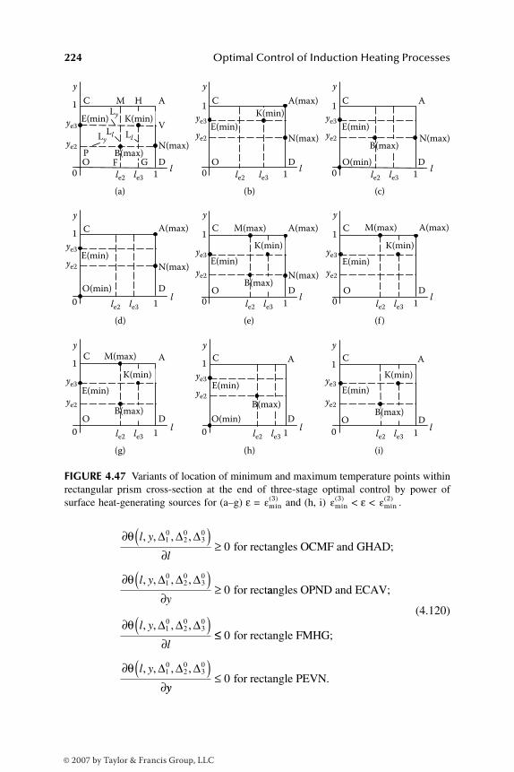
224 Optimal Control of Induction Heating Processes
(4.120)
FIGURE 4.47 Variants of location of minimum and maximum temperature points withinrectangular prism cross-section at the end of three-stage optimal control by power ofsurface heat-generating sources for (a–g) ε = and (h, i) < ε < .
y
ye3
Ly
LyLl Llye2
le2 le3
1
O O O(min)F GP
C CM
M(max)
M(max)
H A
V
D
A(max) C A
D D
N(max)
A(max)
D
N(max)
N(max) N(max)
E(min)
O(min)
C
E(min)
E(min) E(min)K(min)
K(min)
B(max)
1l
le2 le3 1l
A
DO
C
E(min)
le2 le3 1l
le2 le3 1l le2 le3 1
l0
(a) (b) (c)
(d) (e) (f )
(g) (h) (i)
y
ye3
ye2
1
0
y
ye3
ye2
1
0
A
DO(min)
C
E(min)
le2 le3 1l
y
ye3
ye2
1
0
y
ye3
ye2
1
0
O
C A(max) M(max)C A(max)
D O D
N(max)
E(min) E(min)
B(max)
B(max)B(max)
A
O D
C
E(min)
K(min)
le2 le3 1l
y
ye3
ye2
1
0
B(max)
K(min)
K(min)
K(min)
le2 le3 1ll
y
ye3
ye2
1
0 le2 le3 1
y
ye3
ye2
1
0
y
ye3
ye2
1
0
B(max)
εmin3( ) εmin
3( ) εmin2( )
∂ ( )∂
≥θ l y
l
, , , ,∆ ∆ ∆10
20
30
0 for rectangles OCMF and GHAD;
for rect∂ ( )
∂≥
θ l y
y
, , , ,∆ ∆ ∆10
20
30
0 aangles OPND and ECAV;
∂ ( )∂
θ l y
l
, , , ,∆ ∆ ∆10
20
30
≤≤
∂ ( )∂
0
10
20
30
for rectangle FMHG;
θ l y, , , ,∆ ∆ ∆yy
≤ 0 for rectangle PEVN.
DK6039_C004.fm Page 224 Thursday, June 8, 2006 12:34 PM
© 2007 by Taylor & Francis Group, LLC

Optimal Control of Static Induction Heating Processes 225
Obtained correlations allow revealing the profile of the final temperaturedistribution under three-stage control. As it follows from Equation (4.120), duringthe first and the third control stages, the extremum points of minimum temperature(O and E, Κ, respectively) appear on the concurrence of lines Ll and Ly (includingcoordinate axes l = 0 and y = 0). During the second control stage, the extremumpoint B of maximum temperature appears. The maximum temperature can alsobe reached at points M, A, and N along the perimeter of the rectangle; theminimum temperature could appear at points O, E, and Κ.
Therefore, the complete set O, E, Κ, B, M, A, N of seven points consideredas “potential candidates” for points xj
0 is determined. In the next step, it wouldbe necessary to choose particular profiles of final temperature distribution accord-ing to the preset value of ε.
The final temperature distribution can be represented in the form of Expres-sion (4.113). Analysis provided in Rapoport1,19 shows that there might be sixcombinations with maximum number R = 4 of points xj
0 within the prism cross-section. The number, R, exceeds by one the number of optimal control stages, N= 3. Figure 4.47a through Figure 4.47d, and Figure 4.47f through Figure 4.47g,show all possible profiles. The first four profiles represent the condition 1 < β <β* in Equation (4.76). The last two profiles satisfy the condition β > β*, wherethe value β* corresponds to the case of six points xj
0 (Figure 4.47e). Accordingto the basic condition in Equation (3.40), one of these profiles should conformto the case of ε = . In each particular problem, such a profile can be chosenby trial solution of the corresponding set of equations. For the given combinationof four points xj
0, j = the set of equations can be written as:
(4.121)
Here, for the first scenario (Figure 4.47a):
εmin( )3
1 4,
θ θ ε
θ
l y
l y
k10
10
10
20
30 3
20
20
, , , , ;
, ,
*∆ ∆ ∆
∆
( ) − = − ( )
110
20
30 3
30
30
10
20
3
, , ;
, , , ,
*∆ ∆
∆ ∆ ∆
( ) − = − ( )θ ε
θ
k
l y 00 3
40
40
10
20
30 3
( ) − =
( ) − =
( )θ ε
θ θ ε
*
*
;
, , , ,
k
kl y ∆ ∆ ∆ (( )
∂ ( )∂
=
;
, , , , ,, ,θ θl y
l
l ye e e e2 2 10
20
30
2 2 10∆ ∆ ∆ ∆ ∆∆ ∆
∆ ∆ ∆
20
30
3 3 10
20
30
0,
;
, , ,,
( )∂
=
∂ ( )∂
=
y
l y
l
le eθ θ ee ey
y
3 3 10
20
30
0, , ,
.,∆ ∆ ∆( )∂
=
l y y l l y y l l y ye e e e10
10
3 20
3 20
3 30
2 300= = = = = =, , , , , ee el y y2 4
040
21, ,= =
DK6039_C004.fm Page 225 Thursday, June 8, 2006 12:34 PM
© 2007 by Taylor & Francis Group, LLC
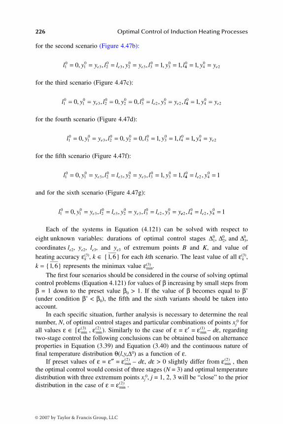
226 Optimal Control of Induction Heating Processes
for the second scenario (Figure 4.47b):
for the third scenario (Figure 4.47c):
for the fourth scenario (Figure 4.47d):
for the fifth scenario (Figure 4.47f):
and for the sixth scenario (Figure 4.47g):
Each of the systems in Equation (4.121) can be solved with respect to
eight unknown variables: durations of optimal control stages ∆1,0 ∆2,
0 and 0∆3,
coordinates le2, ye2, le3, and ye3 of extremum points B and K, and value of
heating accuracy ε(3),k k ∈ for each kth scenario. The least value of all kε(3),
k = represents the minimax value εmin.(3)
The first four scenarios should be considered in the course of solving optimalcontrol problems (Equation 4.121) for values of β increasing by small steps fromβ = 1 down to the preset value β0 > 1. If the value of β becomes equal to β*
(under condition β* < β0), the fifth and the sixth variants should be taken intoaccount.
In each specific situation, further analysis is necessary to determine the realnumber, N, of optimal control stages and particular combinations of points xj
0 forall values ε ∈ [ , ). Similarly to the case of ε = ε′ = – dε, regardingtwo-stage control the following conclusions can be obtained based on alternanceproperties in Equation (3.39) and Equation (3.40) and the continuous nature offinal temperature distribution θ(l,y,∆0) as a function of ε.
If preset values of ε = ε″ = – dε, dε > 0 slightly differ from , thenthe optimal control would consist of three stages (N = 3) and optimal temperaturedistribution with three extremum points xj
0, j = 1, 2, 3 will be “close” to the priordistribution in the case of ε = .
l y y l l y y l y le e e10
10
3 20
3 20
3 30
300 1 1= = = = = =, , , , , , 44
040
21= =, y ye
l y y l y l l y y le e e10
10
3 20
20
30
2 30
20 0 0= = = = = =, , , , , , 440
40
21= =, y ye
l y y l y l y le10
10
3 20
20
30
30
400 0 0 1 1 1= = = = = = =, , , , , , ,, y ye4
02=
l y y l l y y l y le e e10
10
3 20
3 20
3 30
300 1 1= = = = = =, , , , , , 44
02 4
0 1= =l ye ,
l y y l l y y l l y ye e e e10
10
3 20
3 20
3 30
2 300= = = = = =, , , , , ee el l y2 4
02 4
0 1, ,= =
1 6,
1 6,
εmin( )3 εmin
( )2 εmin( )1
εmin( )2 εmin
( )2
εmin( )2
DK6039_C004.fm Page 226 Thursday, June 8, 2006 12:34 PM
© 2007 by Taylor & Francis Group, LLC
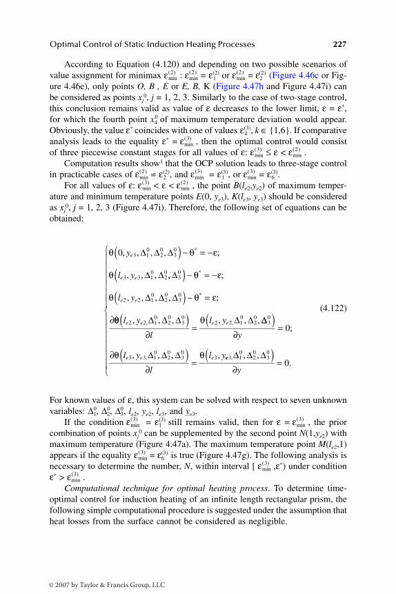
Optimal Control of Static Induction Heating Processes 227
According to Equation (4.120) and depending on two possible scenarios ofvalue assignment for minimax : = 1ε(2) or = ε2
(2) (Figure 4.46c or Fig-ure 4.46e), only points O, B , E or E, B, Κ (Figure 4.47h and Figure 4.47i) canbe considered as points xj
0, j = 1, 2, 3. Similarly to the case of two-stage control,this conclusion remains valid as value of ε decreases to the lower limit, ε = ε*,for which the fourth point x4
0 of maximum temperature deviation would appear.Obviously, the value ε* coincides with one of values kε(3), k ∈ 1,6. If comparativeanalysis leads to the equality ε* = , then the optimal control would consistof three piecewise constant stages for all values of ε: ≤ ε < .
Computation results show1 that the OCP solution leads to three-stage controlin practicable cases of = 2ε(2), and = 1ε(3), or = 6ε(3).
For all values of ε: < ε < , the point B(le2,ye2) of maximum temper-ature and minimum temperature points E(0, ye3), K(le3, ye3) should be consideredas xj
0, j = 1, 2, 3 (Figure 4.47i). Therefore, the following set of equations can beobtained:
(4.122)
For known values of ε, this system can be solved with respect to seven unknownvariables: ∆1,
0 ∆2,0 ∆3,
0 le2, ye2, le3, and ye3.If the condition = ε1
(3) still remains valid, then for ε = , the priorcombination of points xj
0 can be supplemented by the second point N(1,ye2) withmaximum temperature (Figure 4.47a). The maximum temperature point M(le2,1)appears if the equality = ε6
(3) is true (Figure 4.47g). The following analysis isnecessary to determine the number, N, within interval [ ,ε*) under conditionε* > .
Computational technique for optimal heating process. To determine time-optimal control for induction heating of an infinite length rectangular prism, thefollowing simple computational procedure is suggested under the assumption thatheat losses from the surface cannot be considered as negligible.
εmin( )2 εmin
( )2 εmin( )2
εmin( )3
εmin( )3 εmin
( )2
εmin( )2 εmin
( )3 εmin( )3
εmin( )3 εmin
( )2
θ θ ε
θ
0 3 10
20
30
3 3 10
20
, , , , ;
, , ,
*y
l y
e
e e
∆ ∆ ∆
∆ ∆
( ) − = −
,, ;
, , , , ;
*
*
∆
∆ ∆ ∆
30
2 2 10
20
30
( ) − = −
( ) − =
∂
θ ε
θ θ εl ye e
θθ θl y
l
l ye e e e2 2 10
20
30
2 2 10
20, , , , , ,, ,∆ ∆ ∆ ∆ ∆( )
∂=
∆∆
∆ ∆ ∆
30
3 3 10
20
30
3
0( )
∂=
∂ ( )∂
=
y
l y
l
l ye e e
;
, , , ,,θ θ ee
y
3 10
20
30
0, , ,
.∆ ∆ ∆( )∂
=
εmin( )3 εmin
( )3
εmin( )3
εmin( )3
εmin( )3
DK6039_C004.fm Page 227 Thursday, June 8, 2006 12:34 PM
© 2007 by Taylor & Francis Group, LLC
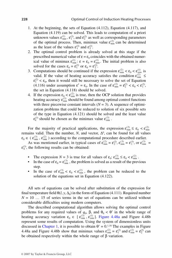
228 Optimal Control of Induction Heating Processes
1. At the beginning, the sets of Equation (4.112), Equation (4.117), andEquation (4.119) can be solved. This leads to computation of a prioriunknown values , 1ε(2), and ε2
(2) as well as corresponding parametersof the optimal process. Then, minimax value can be determinedas the least of the values 1ε(2) and ε(2).2
2. The optimal control problem is already solved at this stage if theprescribed numerical value of ε = ε0 coincides with the obtained numer-ical value of minimax : ε = ε0 = . The initial problem is alsosolved for the cases ε0 = ε1
(2) or ε0 = 2ε(2).3. Computations should be continued if the expression < ε0 < is
valid. If the value of heating accuracy satisfies the condition ≤ε1
(2) < ε0, then it would still be necessary to solve the set of Equation(4.116) under assumption ε′ = ε0. In the case of = ε2
(2) < ε0 < 1ε(2),the set in Equation (4.118) should be solved.
4. If the expression ε0 < is true, then the OCP solution that providesheating accuracy should be found among optimal control functionswith three piecewise constant intervals (N = 3). A sequence of optimi-zation problems that could be reduced to solution of six possible setsof the type in Equation (4.121) should be solved and the least valueεk
(3) should be chosen as the minimax value .
For the majority of practical applications, the expression ≤ ε0 <remains valid. Then the number, N, and vector, ∆0, can be found for all valuesε0 ∈ ( , ) according to the computational procedure described earlier.
As was mentioned earlier, in typical cases of = 2ε(2), = 1ε(3), or =ε(3),6 the following results can be obtained:
• The expression N = 3 is true for all values of ε0: ≤ ε0 < .• In the case of ε0 = , the problem is solved as a result of the previous
step.• In the case of < ε0 < , the problem can be reduced to the
solution of the equations set in Equation (4.122).
All sets of equations can be solved after substitution of the expression forfinal temperature field θ(l, y, ∆0) in the form of Equation (4.111). Required numberN = 10 … 15 of series terms in the set of equations can be utilized withoutconsiderable difficulties using modern computers.
The described computational algorithm allows solving the optimal controlproblems for any required values of q0, β, and θ0 < θ* in the whole range ofheating accuracy variation ε0 ∈ [ , ]. Figure 4.48a and Figure 4.48brepresent some results of computation. Using the system of dimensionless unitsdiscussed in Chapter 1, it is possible to obtain θ* = 0.1,18 The examples in Figure4.48a and Figure 4.48b show that minimax values = ε1
(2) and = ε2(2) can
be obtained respectively within the whole range of β variation.
εmin( )1
εmin( )2
εmin( )1 εmin
( )1
εmin( )2 εmin
( )1
εmin( )2
εmin( )2
εmin( )2
εmin( )3
εmin( )3
εmin( )3 εmin
( )2
εmin( )3 εmin
( )2
εmin( )2 εmin
( )3 εmin( )3
εmin( )3 εmin
( )2
εmin( )3
εmin( )3 εmin
( )2
εmin( )3 εmin
( )1
εmin( )2 εmin
( )2
DK6039_C004.fm Page 228 Thursday, June 8, 2006 12:34 PM
© 2007 by Taylor & Francis Group, LLC

Optimal Control of Static Induction Heating Processes 229
The computations demonstrate that the most typical case of = ε2(2) arises
due to relatively small heat losses from the surface of the heated workpiece. Thecase of = ε1
(2) takes place if the value |q0| increases significantly and if thedifference θ* – θ0 diminishes. If the expression β ≥ βb is valid for ε1
(2) = orε2
(2) = (Figure 4.48a and Figure 4.48b), then the point B that represents themaximum temperature will be located on the side y = 0 of rectangle OCAD;therefore, ye2 = 0 (Figure 4.49).
Figure 4.48c and Figure 4.48d represent optimal heating process parametersin the case of ε0 = . As can be seen, the equality = ε1
(3) is true if β < β*,
FIGURE 4.48 Optimal process parameters as functions of factor β for heating under two-stage (a, b) and three-stage (c, d) control by power of surface heat-generating sources. a:θ0 = –0.1; θ* = 0; q0 = –0.5; (1: 22ε(2); 2: 12ε(2); 3: ∆1
0 for ε0 = 1ε(2) = ; 4: ∆20 for ε0 =
ε1(2 )= ). b: θ0 = –2; θ* = 0; q0 = –0.1; (1: 4ε(2);1 2: 24ε(2); 3: ∆1
0 for ε0 = ε2(2) = ; 4: 2∆0
for ε0 = ε2(2) = ). c: θ0 = –2; θ* = 0; q0 = –0.1; ε0 = (1: 0∆1; 2: 0∆2; 3: ∆3
0 × 103). d:θ0 = –2; θ* = 0; q0 = –0.1 (1: ε0 = 1ε(3); 2: ε0 = 2ε(3); 3: ε0 = 3ε(3), ε0 = 4ε(3); 4: ε0 = ; 5: ε0
= 5ε(3); 6: ε0 = 6ε(3)).
0.4
0.8
0.2
0.6
0
1.0
1 2 3 4
1
2
3
1 2
βb β
β
β
β∗ β∗
βbβb β3
(a) (b)
(c) (d)
4
0.04
0.08
0.12
0.16
0.20
∆0, ε
∆0
∆0, ε
ε
1
2
3
4
0.4
0.8
0.2
0.6
0
1.0
1 2 3 4
1
2
3
4
1 2 3 4
0.04
0.01
0.02
0.03
0.05
1
2
3
4 5
6
εmin( )2
εmin( )2 εmin
( )2
εmin( )2 εmin
( )3
εmin( )2
εmin( )2
εmin( )2
εmin( )2
εmin( )2
εmin( )3 εmin
( )3
DK6039_C004.fm Page 229 Thursday, June 8, 2006 12:34 PM
© 2007 by Taylor & Francis Group, LLC
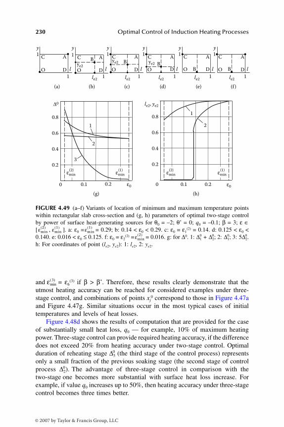
230 Optimal Control of Induction Heating Processes
and = ε6(3) if β > β*. Therefore, these results clearly demonstrate that the
utmost heating accuracy can be reached for considered examples under three-stage control, and combinations of points xj
0 correspond to those in Figure 4.47aand Figure 4.47g. Similar situations occur in the most typical cases of initialtemperatures and levels of heat losses.
Figure 4.48d shows the results of computation that are provided for the caseof substantially small heat loss, q0 — for example, 10% of maximum heatingpower. Three-stage control can provide required heating accuracy, if the differencedoes not exceed 20% from heating accuracy under two-stage control. Optimalduration of reheating stage ∆3
0 (the third stage of the control process) representsonly a small fraction of the previous soaking stage (the second stage of controlprocess ∆2).
0 The advantage of three-stage control in comparison with thetwo-stage one becomes more substantial with surface heat loss increase. Forexample, if value q0 increases up to 50%, then heating accuracy under three-stagecontrol becomes three times better.
FIGURE 4.49 (a–f) Variants of location of minimum and maximum temperature pointswithin rectangular slab cross-section and (g, h) parameters of optimal two-stage controlby power of surface heat-generating sources for θ0 = –2; θ* = 0; q0 = –0.1; β = 3; ε ∈[ , ]. a: ε0 = = 0.29; b: 0.14 < ε0 < 0.29. c: ε0 = ε1
(2) = 0.14. d: 0.125 < ε0 <0.140. e: 0.016 < ε0 ≤ 0.125. f: ε0 = ε2
(2) = = 0.016. g: for ∆0. 1: ∆10 + 0∆2; 2: 0∆1; 3: 05∆2.
h: For coordinates of point (le2, ye2): 1: le2, 2: ye2.
1
y y y y y y
1
(a) (b) (c) (d) (e) (f )
l l l l l l
C A
O D
1
1
C
ye2
ye2 ye2
le2 le2 le2 le2 le2
AB
O D1
1C A
B
O D
1
1
C A
BO D
1
1
C A
BO
1
D
1
C A
BO D
1
2
0.4
0.8
0.2
0.6
0 0.20.1
1
2
3
0
0.4
0.8
∆0
ε0 ε0
0.2
0.6
0.20.1
(g) (h)
le2, ye2
εmin(2) εmin
(2)εmin(1) εmin
(1)
εmin2( ) εmin
1( ) εmin1( )
εmin2( )
εmin( )3
DK6039_C004.fm Page 230 Thursday, June 8, 2006 12:34 PM
© 2007 by Taylor & Francis Group, LLC
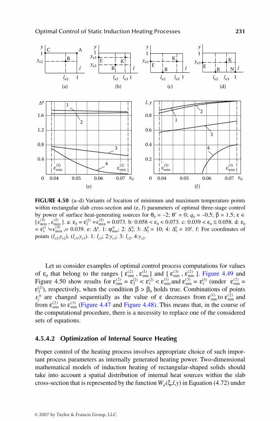
Optimal Control of Static Induction Heating Processes 231
Let us consider examples of optimal control process computations for valuesof ε0 that belong to the ranges [ , ] and [ , ]. Figure 4.49 andFigure 4.50 show results for = ε2
(2) < ε1(2) < and = ε1
(3) (under =ε(2)),2 respectively, when the condition β > βb holds true. Combinations of pointsxj
0 are changed sequentially as the value of ε decreases from to andfrom to (Figure 4.47 and Figure 4.48). This means that, in the course ofthe computational procedure, there is a necessity to replace one of the consideredsets of equations.
4.5.4.2 Optimization of Internal Source Heating
Proper control of the heating process involves appropriate choice of such impor-tant process parameters as internally generated heating power. Two-dimensionalmathematical models of induction heating of rectangular-shaped solids shouldtake into account a spatial distribution of internal heat sources within the slabcross-section that is represented by the function Wd(ξ,l,y) in Equation (4.72) under
FIGURE 4.50 (a–d) Variants of location of minimum and maximum temperature pointswithin rectangular slab cross-section and (e, f) parameters of optimal three-stage controlby power of surface heat-generating sources for θ0 = –2; θ* = 0; q0 = –0.5; β = 1.5; ε ∈[ , ]. a: ε0 = ε2
(2) = = 0.073. b: 0.058 < ε0 < 0.073. c: 0.039 < ε0 ≤ 0.058. d: ε0
= ε1(3 )= ,= 0.039. e: ∆0. 1: 0ϕmin; 2: 0∆1; 3: ∆2
0 × 10; 4: ∆30 × 102. f: For coordinates of
points (le2,ye2), (le3,ye3). 1: le3; 2:ye3; 3: le2, 4:ye2.
1
ye2
le2 le2 le3 le2 le3 le2 le31
C A
B
2
1
3
40.4
0.8
1.2
1.6
0.04 0.05 0.06 ε0 ε0
∆0
0.070
1
B
KE
1
B
K
E
1
B
K
EN
0.4
0.04 0.05 0.06 0.07
0.8
l, y
0.2
0.6
4
2
3
1
0
y1ye3
ye2
y1
ye3
y1
ye3
y
l l l l
εmin(3) εmin
(3)εmin(2) εmin
(2)
(a) (b)
(e) (f )
(c) (d)
εmin3( ) εmin
2( ) εmin2( )
εmin3( )
εmin( )2 εmin
( )1 εmin( )3 εmin
( )2
εmin( )2 εmin
( )1 εmin( )3 εmin
( )2
εmin( )1 εmin
( )2
εmin( )2 εmin
( )3
DK6039_C004.fm Page 231 Thursday, June 8, 2006 12:34 PM
© 2007 by Taylor & Francis Group, LLC

232 Optimal Control of Induction Heating Processes
condition ξ < ∞. Direct solution of the time-optimal problem faces principaldifficulties when function Wd(ξ,l,y) has an arbitrary complex form.
Substantial complication of the OCP solution occurs in comparison with thecase of surface heat-generating sources (Section 4.5.4.1). The shape of temper-ature distribution θ(l,y,∆0) cannot be explicitly defined based on “common sense.”The set of all possible combinations of points xj
0 cannot be revealed dependingon required heating accuracy as was done in the previous section.
Keep in mind, though, that in the general case the computational procedurewill be identical to the one described in Section 3.7, and it can be successfullyapplied to OCP solution for the number of values, ε, descending by small steps.
The following assumptions will be used for the formulation control problem:
1. The function Wd(ξ,l,y) can be defined in arbitrary form.2. The power control u(ϕ) function consists of N piecewise constant
intervals.3. The initial temperature is defined as θ0(l,y) ≡ θ0 = const in Equation
(4.73).4. The boundary condition of the second kind is described by q(y,ϕ) =
qT1(l,ϕ) ≡ q0 = const in Equation (4.74).
Then, similarly to Equation (4.94) and Equation (4.111), the following solutionof the heat conduction equation (Equation 4.72 through Equation 4.74) can bewritten for Γ = 01,17:
DK6039_C004.fm Page 232 Thursday, June 8, 2006 12:34 PM
© 2007 by Taylor & Francis Group, LLC
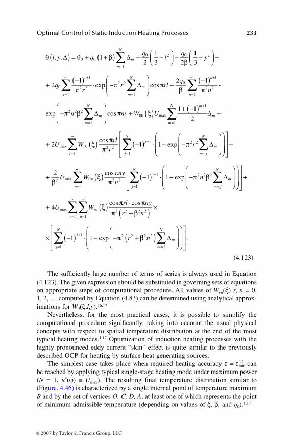
Optimal Control of Static Induction Heating Processes 233
(4.123)
The sufficiently large number of terms of series is always used in Equation(4.123). The given expression should be substituted in governing sets of equationson appropriate steps of computational procedure. All values of Wrn(ξ) r, n = 0,1, 2, … computed by Equation (4.83) can be determined using analytical approx-imations for Wd(ξ,l,y).16,17
Nevertheless, for the most practical cases, it is possible to simplify thecomputational procedure significantly, taking into account the usual physicalconcepts with respect to spatial temperature distribution at the end of the mosttypical heating modes.1,17 Optimization of induction heating processes with thehighly pronounced eddy current “skin” effect is quite similar to the previouslydescribed OCP for heating by surface heat-generating sources.
The simplest case takes place when required heating accuracy ε = canbe reached by applying typical single-stage heating mode under maximum power(N = 1, u*(ϕ) ≡ Umax). The resulting final temperature distribution similar to(Figure. 4.46) is characterized by a single internal point of temperature maximumB and by the set of vertices O, C, D, A, at least one of which represents the pointof minimum admissible temperature (depending on values of ξ, β, and q0).1,17
θ θ βl y qq
lq
m
m
N
, , ∆ ∆( ) = + +( ) − −
−=
∑0 0
1
0 212
13
00 2
0
1
2 2
1
2
213
21
β
ππ
−
+
+−( ) ⋅ −
+
=
∞
∑
y
qr
r
r
exp rr rlq
nm
m
N n
n
2
1
01
2 2
1
2 1∆
=
+
=
∞
∑ ∑
+
−( )cos π
β π⋅⋅
−
+ ( )
=∑exp cos maxπ β π ξ2 2 2
1
001
n ny W Um
m
N
∆++ −( ) +
+ ( )
+
=
=
∑ 1
2
2
1
1
0 2 2
1
m
m
N
m
r
r
U Wrl
r
∆
maxcosξ ππ
∞∞+
=∑ ∑−( ) ⋅ − −
1 1
1 2 2jm
m j
N
rexp π ∆
+
+ ( )
=
=
∑j
N
n
n
U Wny
n
1
2 0 2 2
1
2β
ξ ππmax
cos∞∞
+
=∑ ∑−( ) ⋅ − −
1 1
1 2 2 2jm
m j
N
nexp π β ∆
+
+ ( )
=
=
∞
=
∞
∑
∑∑
j
N
rn
nr
U W
1
11
4 maxcosξ ππ ππ β
π
rl ny
r n
rj
⋅+( ) ×
× −( ) ⋅ − − ++
cos
exp
2 2 2 2
1 2 21 1 ββ2 2
1
n m
m j
N
j
N
( )
==∑∑ ∆ ..
εmin( )1
DK6039_C004.fm Page 233 Thursday, June 8, 2006 12:34 PM
© 2007 by Taylor & Francis Group, LLC

234 Optimal Control of Induction Heating Processes
In the real-life process of induction slab heating (in particular, heating ofnonmagnetic materials), the parameter ξ takes on limiting values in expressionsfor Wd(ξ,l,y) in Equation (4.72). These values differ significantly from each other.
If the parameter ξ is substantially small, meeting the condition ≤ 1.5, then
the rectangle corner A turns out to be the least heated area.1,16,17 Only the pointsA and B can be considered in this case as x1
0 and x20 according to the properties
in Equation (3.39) and Equation (3.40) for ε = (Figure 4.51a).The set of governing equations resulting from Equation (3.39) and Equation
(3.40) for ε = under N = 1 can be written as follows:
(4.124)
After substituting θ(l,y,∆0) in the form of Equation (4.123) under N = 1, thissystem can be solved with respect to unknown variables ∆0, , le2, and ye2. Sucha situation arises, for example, when heating titanium alloys slabs before rolling(the applied frequency is 50 Hz).1,16,17
As a rule, the value represents the utmost attainable accuracy that cannotbe further improved by increasing the number, N, of constancy interval of functionu*(ϕ).1,17 This means that the expression = εinf will be valid. Therefore, if therequired heating accuracy ε0 coincides with minimax value , then the time-optimal control problem is reduced to solving the set of equations in Equation
FIGURE 4.51 Variants of location of minimum and maximum temperature points withinrectangular slab cross-section at the end of internal source heating with constant power
for ≤ 1.5 (a) and > 1.5 (b).
0 1l l
y
ye2
y
ye2
le2 le2
O
C
B(max)
A(min)
D
0 1
1
O(min)
C
B(max)
A
D
1
(a) (b)
β ξ2
------- β ξ2
-------
βξ2
-------
εmin( )1
εmin( )1
θ θ ε
θ θ ε
l ye e2 20 1
0
1
11 1
, , ;
, ,
*min
*m
∆
∆
( ) − =
( ) − = −
( )
iin ;
, , , ,
1
2 20
2 20
1 1
( )
∂ ( )∂
=∂ ( )
∂=
θ θl y
l
l y
y
e e e e∆ ∆00.
εmin( )1
εmin( )1
εmin( )1
εmin( )1
DK6039_C004.fm Page 234 Thursday, June 8, 2006 12:34 PM
© 2007 by Taylor & Francis Group, LLC
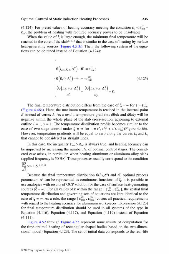
Optimal Control of Static Induction Heating Processes 235
(4.124). For preset values of heating accuracy meeting the condition ε0 < =εinf, the problem of heating with required accuracy proves to be unsolvable.
When the value of ξ is large enough, the minimum final temperature will bereached in the core of the slab1,16,17 that is similar to the case of heating by surfaceheat-generating sources (Figure 4.51b). Then, the following system of the equa-tions can be obtained instead of Equation (4.124):
(4.125)
The final temperature distribution differs from the case of ξ = ∞ for ε =(Figure 4.46a). Here, the maximum temperature is reached in the internal pointB instead of vertex A. As a result, temperature gradients ∂θ/∂l and ∂θ/∂y will benegative within the whole plane of the slab cross-section, adjoining to externaloutline l = 1, y = 1. The temperature distribution profile becomes similar to thecase of two-stage control under ξ = ∞ for ε = ε′, ε(2)
1 < ε′< (Figure 4.46b).However, temperature gradients will be equal to zero along the curves Ll and Ly
that cannot be considered as straight lines.
In this case, the inequality > εinf is always true, and heating accuracy canbe improved by increasing the number, N, of optimal control stages. The consid-ered case arises, in particular, when heating aluminum or aluminum alloy slabs(applied frequency is 50 Hz). These processes usually correspond to the condition
>> 1.5.1,16,17
Because the final temperature distribution θ(l,y,∆0) and all optimal processparameters ∆0 can be represented as continuous functions of ξ, it is possible touse analogies with results of OCP solution for the case of surface heat-generatingsources (ξ = ∞). For all values of ε within the range [ , ], the spatial finaltemperature distribution and governing sets of equations are kept identical to thecase of ξ = ∞. As a rule, the range [ , ] covers all practical requirementswith regard to the heating accuracy for aluminum workpieces. Expression (4.123)for final temperature distribution should be used in all systems of the type inEquation (4.116), Equation (4.117), and Equation (4.119) instead of Equation(4.111).
Figure 4.52 through Figure 4.55 represent some results of computation forthe time-optimal heating of rectangular-shaped bodies based on the two-dimen-sional model (Equation 4.123). The set of initial data corresponds to the real-life
εmin( )1
θ θ ε
θ θ ε
l ye e2 20 1
0
1
10 0
, , ;
, ,
*min
*m
∆
∆
( ) − =
( ) − = −
( )
iin ;
, , , ,
1
2 20
2 20
1 1
( )
∂ ( )∂
=∂ ( )
∂=
θ θl y
l
l y
y
e e e e∆ ∆00.
εmin( )1
εmin( )1
εmin( )1
βξ2
-------
εmin( )2 εmin
( )1
εmin( )2 εmin
( )1
DK6039_C004.fm Page 235 Thursday, June 8, 2006 12:34 PM
© 2007 by Taylor & Francis Group, LLC
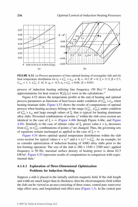
236 Optimal Control of Induction Heating Processes
process of induction heating utilizing line frequency (50 Hz).1,16 Analyticalapproximations for heat sources Wd(ξ,l,y) were in the calculations.17
Figure 4.52 shows the temperature profile at the end of heating and optimalprocess parameters as functions of heat losses under condition of = εinf whenheating titanium slabs. Figure 4.53 shows the results of computations of optimalprocess when heating accuracy belongs to the range [ , ], under conditionof > εinf and large enough values of ξ, that is typical for heating aluminumalloy slabs. Presented combinations of points xj
0 within the slab cross-section areidentical to the case of ξ = ∞ (Figure 4.46b through Figure 4.46e, and Figure4.49). Similarly to the case of infinite value of ξ, preset value ε = ε0 decreasesfrom to ; combinations of points xj
0 are changed. Thus, the governing setsof equations remain unchanged as applied to the case of ξ = ∞.
Figure 4.54 shows optimal spatial temperature distributions within the slabcross-section for typical values ε = ε1
(2) and ε = ε2(2) = . As an example, let
us consider optimization of induction heating of AMG alloy slabs prior to thehot forming operation. The size of the slab is 280 × 1540 × 2300 mm3; appliedfrequency is 50 Hz; maximal surface density of heating power is about 82.5kW/m2. Figure 4.55 represents results of computations in comparison with exper-imental data.1
4.5.4.3 Exploration of Three-Dimensional Optimization Problems for Induction Heating
Suppose a slab is placed in the initially uniform magnetic field. If the slab lengthand width are much larger than its thickness, then the electromagnetic field withinthe slab can be viewed as an area consisting of three zones: central part, transverseedge effect area, and longitudinal end effect area (Figure 1.3). In the central part
FIGURE 4.52 (a) Process parameters of time-optimal heating of rectangular slab and (b)final temperature distribution for ε0 = = εinf. a: θ0 = –0.2; θ* = 0; ξ = 11.3; β = 5.7;Umax = 1; 1: ; 2: 0∆1. b: q0 = –0.3; ε0 = = 0.08; ∆1
0 = 0.053.
0 0.05 0.10 0.15 0.20
(a) (b)
0.25|q0|
0.01
0.02
0.03
0.04
0.05
0.06
0.07
1
2
0.2 0.4 0.8
l0.6
0.2
0.4
0.6
0.8
0
Bye2
le2
A
0.04
−0.04
0.08
−0.08
θ − θ∗y
εmin( )1
εmin( )1 εmin
( )1
εmin( )1
εmin( )2 εmin
( )1
εmin( )1
εmin( )1 εmin
( )2
εmin( )2
DK6039_C004.fm Page 236 Thursday, June 8, 2006 12:34 PM
© 2007 by Taylor & Francis Group, LLC

Optimal Control of Static Induction Heating Processes 237
of the slab, the emf distribution corresponds to the field in the infinite plate.Basically, end and edge effects have a two-dimensional space distribution exclud-ing only the zone of three-dimensional corners where the field is three dimen-sional representing a mixture of the end and edge effects.
The electromagnetic edge effect is typically negligible when heating cylin-drical workpieces. However, this effect can play an essential role for manypractical applications such as induction heating of slabs before rolling. In these
FIGURE 4.53 (a–f) Variants of location of minimum and maximum temperature pointsand (g) optimal process parameters for time-optimal heating of rectangular prism for > εinf (θ0 = –0.95; θ* = 0; Umax = 1; q0 = –0.1; ξ = 52.3; β = 5.5; ε0 ∈ [ , )). a: ε0
= = 0.15. b: 0.104 < ε0 < 0.150. c: ε0 = ε1(2) = 0.104. d: 0.0984 < ε0 < 0.1040. e:
0.012 < ε0 ≤ 0.0984. f: ε0 = ε2(2) = = 0.012.
1 y
ye2
le2
ye2
le2 le2
le2
le2, ye2
ye2
le2
ye2
le2
ye2
le2
y y
y y y
C
B
A
D
1
(a) (b) (c)
(d) (e)
(g)
(f )
0
1 C
B
A
D
1
0
1 C
B
A
D
1
0
1 C
B
A
D
1
0
1 C
B
A
1
0
1 C
B
A
1
0
0.2
0.4
0.6
0.8
0.04 0.08
0.15
0.12
0.05
0.10
ε0
l l l
l l l
εmin(2) εmin
(1)
Δ20
Δ10
Δ10, Δ2
0
εmin1( )
εmin2( ) εmin
1( )
εmin1( )
εmin2( )
DK6039_C004.fm Page 237 Thursday, June 8, 2006 12:34 PM
© 2007 by Taylor & Francis Group, LLC
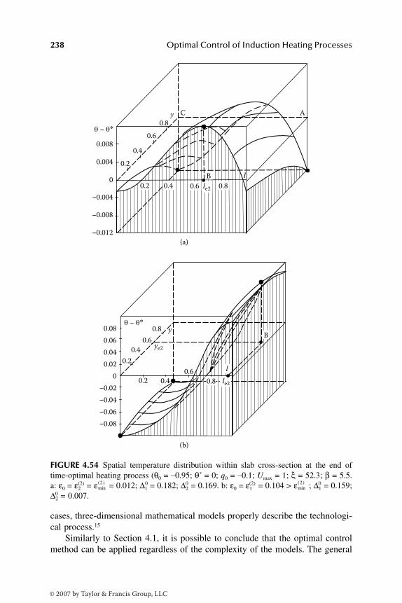
238 Optimal Control of Induction Heating Processes
cases, three-dimensional mathematical models properly describe the technologi-cal process.15
Similarly to Section 4.1, it is possible to conclude that the optimal controlmethod can be applied regardless of the complexity of the models. The general
FIGURE 4.54 Spatial temperature distribution within slab cross-section at the end oftime-optimal heating process (θ0 = –0.95; θ* = 0; q0 = –0.1; Umax = 1; ξ = 52.3; β = 5.5.a: ε0 = ε2
(2) = = 0.012; ∆10 = 0.182; ∆2
0 = 0.169. b: ε0 = ε1(2) = 0.104 > ; ∆1
0 = 0.159;∆2
0 = 0.007.
0.2
0.4
0.6
0.8
0.2 0.4 0.8
l
0.6 0
0.004
−0.004
0.008
θ − θ∗
θ − θ∗
−0.008
−0.012
(a)
C y
B
A
0.2 0.4 0.8
0.6 l 0.2
0.4
0.6
0.8 y
ye2
le2
B
0
0.04
−0.04
−0.02
0.02
0.06
0.08
−0.06
−0.08
(b)
le2
εmin( )2 εmin
( )2
DK6039_C004.fm Page 238 Thursday, June 8, 2006 12:34 PM
© 2007 by Taylor & Francis Group, LLC
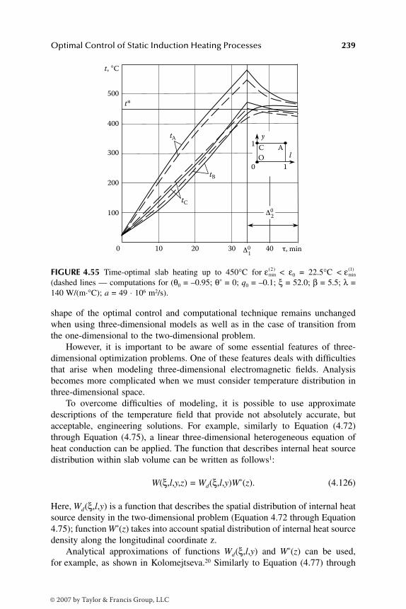
Optimal Control of Static Induction Heating Processes 239
shape of the optimal control and computational technique remains unchangedwhen using three-dimensional models as well as in the case of transition fromthe one-dimensional to the two-dimensional problem.
However, it is important to be aware of some essential features of three-dimensional optimization problems. One of these features deals with difficultiesthat arise when modeling three-dimensional electromagnetic fields. Analysisbecomes more complicated when we must consider temperature distribution inthree-dimensional space.
To overcome difficulties of modeling, it is possible to use approximatedescriptions of the temperature field that provide not absolutely accurate, butacceptable, engineering solutions. For example, similarly to Equation (4.72)through Equation (4.75), a linear three-dimensional heterogeneous equation ofheat conduction can be applied. The function that describes internal heat sourcedistribution within slab volume can be written as follows1:
W(ξ,l,y,z) = Wd(ξ,l,y)W*(z). (4.126)
Here, Wd(ξ,l,y) is a function that describes the spatial distribution of internal heatsource density in the two-dimensional problem (Equation 4.72 through Equation4.75); function W*(z) takes into account spatial distribution of internal heat sourcedensity along the longitudinal coordinate z.
Analytical approximations of functions Wd(ξ,l,y) and W*(z) can be used,for example, as shown in Kolomejtseva.20 Similarly to Equation (4.77) through
FIGURE 4.55 Time-optimal slab heating up to 450°C for < ε0 = 22.5°C <(dashed lines — computations for (θ0 = –0.95; θ* = 0; q0 = –0.1; ξ = 52.0; β = 5.5; λ =140 W/(m·°C); a = 49 ⋅ 106 m2/s).
1
l
y 1
0
O
C A
100
0
200
300
400
500
t, °C
10 20 30 40 τ, min
t∗
tA
tC
tB
Δ02
Δ01
εmin( )2 εmin
( )1
DK6039_C004.fm Page 239 Thursday, June 8, 2006 12:34 PM
© 2007 by Taylor & Francis Group, LLC
240 Optimal Control of Induction Heating Processes
Equation (4.91), and Equation (4.123), analytical models of three-dimensionaltemperature fields can be found for arbitrary and, in particular, stepwise heatpower control functions. In the case of a pronounced eddy current “skin” effect,the simplified model can be applied for required heating accuracy ε = ε0 ≥ .Similarly to the two-dimensional case, this model takes into account heat-gener-ating sources within the slab surface layer. Similarly to the two-dimensional case,representation of function W(ξ,l,y,z) in the form of Equation (4.126) allowsdeveloping the governing set of equations using basic alternance properties (Equa-tion 3.39 and Equation 3.40).
Within each rectangular cross-section, an area that can be considered as apotential “candidate” for points xj
0 can be found in the same manner as in the two-dimensional problem considered above. Because points xj
0 are located in differentcross-sections, the appropriate computational sets should be supplemented by equa-tions determining axial coordinates of these points (similarly to what was discussedin Section 4.5.3 for cylindrical billets). Based on results obtained in Section 4.5.4.1and using the linearized three-dimensional model for heating by surface sources,the described analysis has been performed in the course of a computational proce-dure for time-optimal heating of aluminum alloy slabs.1
4.6 OPTIMAL CONTROL FOR COMPLICATED MODELS OF THE INDUCTION HEATING PROCESS
4.6.1 OVERVIEW
Generally speaking, space–time temperature distribution within the heated work-piece is described by a highly complex mathematical model of interrelated Max-well and Fourier equations for electromagnetic and temperature fields, respec-tively (Section 1.2.1). The inherently nonlinear nature of the induction heatingprocess implies nonlinearity of the model that takes into consideration importantfeatures of induction heating processes, including end and edge effects, nonlinearmaterial properties, nonlinear nature of boundary conditions, etc.
The solution of nonlinear interrelated electrothermal equations by rathercumbersome numerical methods represents a separate topic. In this case, the setof equations cannot be solved analytically but approximate solutions can be foundwith the accuracy that a properly designed and applied model provides. Devel-opment of modern computers leads to widespread use of effective numericalmethods offering maximal advantages of computation of interrelated electromag-netic and heat transfer problems.1,15
This section will detail how the alternance method can be extended onto thewide range of optimization problems for complicated numerical models. It isimportant to clarify whether the shape of optimal control algorithms for thesimplified IHP models can be transferred into these more complex cases. Gen-erally speaking, the nonlinear nature of the induction heating process affects thechoice of optimal control algorithm. To obtain optimal solution, it is necessaryto apply an exact statement to each particular case of the optimal control problem.
εmin( )2
DK6039_C004.fm Page 240 Thursday, June 8, 2006 12:34 PM
© 2007 by Taylor & Francis Group, LLC
Optimal Control of Static Induction Heating Processes 241
Nevertheless, detailed analysis shows1 that, in most cases, suitable practicalsolutions found for linear models remain valid for nonlinear numerical models.
It is possible to prove mathematically1 that the time-optimal control consistsof alternating stages of heating with maximum power u ≡ Umax (heat ON) andsubsequent soaking under u ≡ 0 (heat OFF) cycles regardless of nonlinearity,dimensionality, and other specifics of applied models. Consequently, optimalcontrol u*(ϕ) can be written in the form of a stepwise function (Equation 2.27)(Figure 2.8). Additional constraints lead to a number of essential features andcomplications of optimal control in the same manner as for linear models (Section4.1).
Similar conclusions can be drawn for the wider range of optimal controlproblems, using piecewise linear approximation of equations describing theinduction system under control. As a rule, such approximation provides temper-ature field description by a set of heat conduction equations for each time interval.Accuracy of approximation is fair when the number of time steps is largeenough.1,7,21 Then, optimal controls on appropriate time intervals can be deter-mined for corresponding linear models. The linkage of control functions onseparate intervals into the general control algorithm leads to an optimal solutionidentical to optimal control for the linear single-equation model of the heatingprocess.
Because the optimal control is kept unchanged, the shape of final spatialtemperature distribution is kept identical as well. In other words, similar-by-shapetemperature distributions can be considered as outputs obtained in response tosimilar-by-form optimal control inputs. This conclusion remains correct for heat-ing process models of different complexity.
As a result, it is possible to conclude that, in the most practical cases, generalqualitative features of optimal processes discussed earlier for the simplified IHPmodels remain valid for complex mathematical models. This means that thealternance method can be successfully applied for a wide variety of specific IHPoptimization problems for complicated heating models.
Similarly to OCP solution for linear models, the shape of the optimal controlalgorithm is known, but the number, N, and the values ∆1, ∆2, …, ∆N remainunknown. The task of vector ∆0 = (∆1
0, ∆20, …, ∆0
N) search is reduced to theproblem of mathematical programming (Equation 3.38) that can be solved on thebase of general correlations in Equation (3.39) and Equation (3.40). The sets ofgoverning equations are similar to the linear case, but the solving procedurediffers significantly from the cases described earlier because it is impossible toobtain an exact expression for the temperature field as a function of vector ∆.Here, approximate analytical or numerical methods are applicable to simulate theheating process. Both techniques will be used later on the base of proposedmethod for two typical time-optimal control problems.
DK6039_C004.fm Page 241 Thursday, June 8, 2006 12:34 PM
© 2007 by Taylor & Francis Group, LLC

242 Optimal Control of Induction Heating Processes
4.6.2 APPROXIMATE METHOD FOR COMPUTATION OF THE OPTIMAL INDUCTION HEATING PROCESS FOR FERROMAGNETIC BILLETS
The heating processes for ferromagnetic billets are widely used in numerousadvanced technologies; however, they are the most complex because of theirnonlinearity. Nonlinear effects due to temperature dependency of magnetic per-meability result in the transition between ferromagnetic and paramagnetic phasesof heated material at the Curie point.7,15,21 These phenomena lead to significantchanges in intensity and spatial distribution of internal heat sources during theheating process. Additionally, temperature dependencies of electromagnetic andthermophysical characteristics affect the temperature field significantly.
In a number of typical cases, the process of ferromagnetic billet heating canbe represented with acceptable-in-practice accuracy as a piecewise linear pro-cess.1,7,21 The heating process can be divided into “cold,” “intermediate,” and“hot” stages. Within each stage, a temperature field can be represented by thetransfer equation with corresponding boundary conditions. The values of ther-mophysical characteristics of the heated material, spatial distribution of internalheat sources, and constraints on control inputs will be noticeably different duringthese stages.1
During the cold stage, the heated materials exhibit magnetic properties. Inthe intermediate stage, at temperatures below the Curie point, the magneticmoments are partially aligned within the magnetic domain in ferromagneticmaterials. As the temperature increases from below the Curie point, thermalfluctuations increasingly destroy this alignment, until the net magnetizationbecomes zero at and above the Curie point. On the hot stage above the Curiepoint, the material is purely paramagnetic.
It is possible to show1,7 that the temperature distribution during the heatingprocess can be described by linear equation with respect to relative units underboundary conditions of the second kind in the form of Equation (1.27) throughEquation (1.35) for the one-dimensional case or Equation (4.72) through Equation(4.74) for the two-dimensional case. At transition from stage to stage, the utmostmaximum values of heating power Umax and functions W(ξ,l) (or W(ξ,l,y)) willbe changed in the stepwise manner1 that reflects stepwise changes in billetmagnetic properties.
The induction heating process will be adequately represented by the describedmathematical model under boundary conditions of the third kind (Equation 1.34or Equation 4.75), if the heat loss level (the value of the Biot number) remainsconstant during the whole process.1,7
Similarly to the preceding case, the induction heating process for the non-magnetic slabs can be described by a piecewise linear model when other nonlinearthermophysical properties should be taken into account. The resulting linearizedrepresentation of the heating process allows one to extend an optimal controlmethod (developed for linear models) to nonlinear optimization problems.
DK6039_C004.fm Page 242 Thursday, June 8, 2006 12:34 PM
© 2007 by Taylor & Francis Group, LLC

Optimal Control of Static Induction Heating Processes 243
As was shown earlier, the time-optimal heating power control consists ofalternating stages of heating with maximum power u ≡ Umax (heat ON) andsubsequent soaking under u ≡ 0 (heat OFF) cycles. The number, N ≥ 1, of stagesis defined uniquely by given heating accuracy ε and increases with decreasing ε.Therefore, the shape of the optimal control algorithm is known, but the numberof stages, N, and durations, ∆1, ∆2, …, ∆N, of those stages remains unknown. Theexpression for final temperature distribution θ(l, ∆) can be written in the explicitform as a function of spatial coordinate l and vector ∆ similarly to Equation(2.28), Equation (4.15), and Equation (4.34). However, here the necessity arisesto examine a positional relationship between borders of linearity intervals andoptimal control intervals. As a rule, this additional problem can be solved basedon physical features of optimal induction heating processes or using the successiveapproximations method.
Let us consider a typical problem of a time-optimal process for static induc-tion heating of ferromagnetic billets to the temperature above the Curie point.The temperature should be constrained by a certain maximum level. Similarly tothe case of the one-dimensional linear model in Equation (4.3), the typicalalgorithm of time-optimal heat power control can be obtained in the followingform if the constraint on maximum temperature is taken into account:
(4.127)
Because constraint on thermal stress is neglected, the maximum heatingpower can be applied until the moment ϕθ, when the temperature reaches itslimitation. In contrast to the algorithm in Equation (4.3), the maximum admissiblelevel of heating power Umax will be changed in a stepwise manner over transitionfrom the cold stage (0 < ϕ < ϕmax1) to the intermediate stage (ϕmax1 < ϕ < ϕmax2)and then to the hot stage (ϕ > ϕmax2). During each of these stages, Umax will beequal to one of preset constant values Umax1, Umax2, and Umax3, respectively.7,21
This interval is over at a certain moment ϕ = ϕθ when temperature maximumbecomes equal to admissible value θadm. The hot stage also includes time interval(ϕθ,∆1
0) of temperature holding at the maximum level and the next alternatingstages of heating with maximum power Umax3 and temperature soaking.
u
U
U
U*
max max
max max max
, ;
, ;
ϕ
ϕ ϕ
ϕ ϕ ϕ
( ) =
< <
< <
1 1
2 1 2
0
mmax max
max
, ;
, ;
3 2
10
3
21 1
ϕ ϕ ϕ
ϕ ϕ ϕ
θ
θθ
< <
( ) < <
+ −(
u
U
∆
))
< < =
+−
jj j j N
11 2 3, , , , ..., .ϕ ϕ ϕ
DK6039_C004.fm Page 243 Thursday, June 8, 2006 12:34 PM
© 2007 by Taylor & Francis Group, LLC
244 Optimal Control of Induction Heating Processes
During the interval (ϕθ,∆10), temperature maximum will be held at the max-
imum admissible level by applying control input uθ(ϕ). The holding control uθ(ϕ)can be described approximately by Expression (4.13) under boundary conditionsof the third kind for constant value Bi in Equation (1.34). After substitution ofuθ(ϕ) in the form of Equation (4.13) into Equation (4.15) and Equation (4.16) itis possible to obtain the expression for final temperature distribution θ(l,∆). Bysubstituting control input of the type in Equation (4.127) into solution of generalheat transfer Equation (1.36) and calculating appropriate integrals, it is possibleto obtain the final temperature distribution in the following form with respect tothe simplified one-dimensional model1:
(4.128)
Relative units can be calculated by Equation (1.28), Equation (1.29), Equation(1.33), and Equation (1.35) with regard to parameters of the hot stage undermaximum specific power of internal heat sources Pmax = Pmax3. The followingdenotations are used in Expression (4.128):
1. Wn(v), v = 1, 2, 3 represent coefficients Wn(ξ) calculated by the formula
in Equation (1.45) for known functions W(ξ,l) during the cold (v = 1),intermediate (v = 2), and hot (v = 3) stages, respectively.7,21
2. Factors γ1 and γ2 can be defined by correlations:
. (4.129)
3. The values Umax1 and Umax2, can be computed from formulas:
θ θµ
µ µl
K l
Bi Bi K
n
n nn
, ∆Γ
( ) = + ( )+ + −( ) ( )0 2 2 2
2
1==
∞
( ) ( )
∑ ×
× −( ) +1
11
222
12
1γ γµ ϕ µ ϕW e W en nn nmax max 22
21
2 223
−( ) +
+ −( )( )
e
W e e
n
n nn
µ ϕ
µ ϕ µ ϕθ
max
max ++ −( ) +
+−
( )
( )
W a e e
W be
n
n n
n
n n3
3 2
2
21
2
θµ µ ϕ
θ
θ
θ
µµ β
∆
µµ β ϕ µ ϕµ
θ θ θn nn m
m
N
e e
W
21 1
22
1∆ ∆∆
− −( )−
−( )
∑
+
=
nn
j
Nj
en m
m j
N
3
3
11 1
2
( )
=
+−
∑ −( ) −∑
=µ ∆
.
γ λλ
γ λλ1
3
11 2
3
22= =U Umax max;
DK6039_C004.fm Page 244 Thursday, June 8, 2006 12:34 PM
© 2007 by Taylor & Francis Group, LLC

Optimal Control of Static Induction Heating Processes 245
, (4.130)
where λv , Pmaxv , v = 1, 2, 3 are given values of thermal conductivity and maximumspecific power of internal heat sources during appropriate stages of the heatingprocess. The value ϕθ can be found using the computational technique describedin Section 4.1.2. Times ϕmax1 and ϕmax2 represent the borders of appropriatelinearity intervals.7,21
If required heating accuracy is preset, the considered optimal control problemcan be reduced to search for a vector of unknown parameters ∆0. The problemcan be solved using a technique that differs from the case of linear models (Section4.1.2) only by the fact that Expression (4.128) should be used for θ(l,∆0) in theequations sets.
As an example, let us consider a typical problem of time-optimal control ofthe induction heating process for steel cylindrical billets. Computations have beenperformed according to the previously described technique with respect to initialdata presented in Table 4.2 under X = 0.02 m; t0 = 20°C; t* = 1200°C; f = 50 Hz;and Bi = 0.1. Expression for final temperature distribution θ(l,∆0) in the form ofEquation (4.128) was used in sets of equations. This example shows the optimalcontrol mode when it is necessary to provide maximum heating accuracy ε =
. Figure 4.56 clearly shows that the difference between control algorithms inEquation (4.127) and Equation (4.3) lies in stepwise variation of maximum powerduring the first control interval until the maximum temperature reaches its utmostadmissible value. In this case, the shape of final temperature distribution alongthe billet radius and its properties remain unchanged in comparison with the caseof linear models.
4.6.3 OPTIMAL CONTROL FOR NUMERICAL MODELS OF INDUCTION HEATING PROCESSES
Highly effective numerical methods are widely and successfully used in thecomputation of interrelated electromagnetic and heat transfer problems of differ-ent complexity. Modern electroheat numerical computation techniques allow
TABLE 4.2Computation of Time-Optimal Control for Induction Heating of Steel Cylindrical Billets
Initial Data
Heating Stage λ,W/(m·°C) a·104,m2/sec P0max,κW/m2
ColdIntermediateHot
48.134.330.5
0.0930.0660.055
446332141965
UP
PU
P
PUmax
max
maxmax
max
maxmax; ;1
1
32
2
33 1= = =
εmin( )2
DK6039_C004.fm Page 245 Thursday, June 8, 2006 12:34 PM
© 2007 by Taylor & Francis Group, LLC
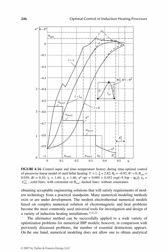
246 Optimal Control of Induction Heating Processes
obtaining acceptable engineering solutions that will satisfy requirements of mod-ern technology from a practical standpoint. Many numerical modeling methodsexist or are under development. The modern electrothermal numerical modelsbased on complex numerical solution of electromagnetic and heat problemsbecome the most commonly used universal tools for investigation and design ofa variety of induction heating installations.15,21,22
The alternance method can be successfully applied to a wide variety ofoptimization problems for numerical IHP models; however, in comparison withpreviously discussed problems, the number of essential distinctions appears.On the one hand, numerical modeling does not allow one to obtain analytical
FIGURE 4.56 Control input and time–temperature history during time-optimal controlof piecewise linear model of steel billet heating: Γ = 1; ξ = 2.82; θ0 = –0.92; θ* = 0; θadm =0.039; Bi = 0.10; γ1 = 1.44; γ2 = 1.46; uθ (ϕ) = 0.094 + 0.452 exp[–9.3(ϕ – ϕθ)]; ε0 =
; solid lines: with constraint on θmax; dashed lines: without constraints.
0
u∗
−1
−0.1
−0.2
−0.3
−0.4
−0.5
−0.6
−0.7
−0.8
−0.9
1
2
3
0 0 0.1 0.2 0.3 0.4 0.5 ϕ
0 1
θ − θ∗
θadm
umax1
umax2
umax3
u∗
uθ
Δ02
Δ01
ϕθϕmax2ϕmax1
l = 1
l = 0
l = le2
le2
l
θ(l, Δ0) − θ∗
εmin( )2
DK6039_C004.fm Page 246 Thursday, June 8, 2006 12:34 PM
© 2007 by Taylor & Francis Group, LLC

Optimal Control of Static Induction Heating Processes 247
expressions for temperature fields; therefore, the final temperature distributiont(x,∆) cannot be represented in the explicit form as a function of spatial coordi-nates and vector of unknown parameters.
On the other hand, according to the alternance method, solution of equationssets can be obtained by an iterative technique (see Section 3.4) that requiresrepeated calls for the numerical model. This can result in an increasing amountof required computations that can prove to be inadmissible. It is more effectiveto find an extremum of the auxiliary function IP(∆) within the space of unknownparameters ∆i, i = .1,15 The auxiliary problem is equivalent to the initial oneif the auxiliary function IP(∆) is chosen in such a way that its global minimumis equal to zero for the optimal values of sought parameters ∆i, i = .
In this case a function IP(∆) can be considered as the sum of linear combi-nations of final temperatures t(xj
0,∆). Variables xj0 represent coordinates of points
where maximum admissible deviations of final temperature from the desired oneare reached. These combinations can be obtained as a result of the algebraicaddition of the left-hand sides of the equations in the equations set. All of thesecombinations tend to zero under optimal values of the vector ∆ = ∆0. For particularapplication, the appropriate set of equations should be chosen and solved. Theproper choice of the set of equations can be performed using additional informa-tion with respect to temperature distribution during the optimal processes subjectto simplified linear models of the controlled heating process.
To calculate temperatures t(xj0,∆), it is necessary to define the expression
t(xj0,τ) for temperature at the point xj
0 during process time τ under control inputuniquely specified by the vector ∆. If the function t(xj
0,τ) is found, then, for anyvector ∆, it is possible to obtain the expression t(xj
0,∆) = t(xj0,τ0), where the value
of τ0 is equal to total heating process time. The problem of definition t(xj0,τ) can
be solved using numerical models. The orthogonal mesh discretizes the area ofmodeling into the certain array of nodes. The numerical models allow one tocalculate the maximum tmax or minimum tmin temperatures at nodes of the spatialmesh in any required time point. The computational procedure often becomessimpler if additional information with regard to location of points xj
0 is employed.The described computational procedure can be reduced to the definition of
dependencies tmax(τ) and tmin(τ), and tmax(∆) and tmin(∆), respectively, instead oft(xj
0,τ) and t(xj0,∆). Search of function IP(∆) minimum is performed using known
numerical methods. Reduction of required computations is provided if simpleanalytical approximations of tmax(τ) and tmin(τ) are used to diminish the numberof calls for numerical models.15 Approximations of functions tmax(τ) and tmin(τ)can be written in the polynomial form according to the method of least squares.Then the computational procedure represents the sequence of optimization prob-lems that could be reduced to minimization of function Ip(∆).
This procedure typically exhibits fast convergence. In each iteration step, theanalytical approximations are refined with respect to expressions for temperaturecalculated by the numerical model under ∆0. Here, the value of ∆0 is obtained asa result of the previous step. The described iteration procedure is repeated untilvalues of sought parameters ∆i,
0 i = will coincide satisfactorily with the
1 N,
1 N,
1 N,
DK6039_C004.fm Page 247 Thursday, June 8, 2006 12:34 PM
© 2007 by Taylor & Francis Group, LLC

248 Optimal Control of Induction Heating Processes
values of the previous step. The initial values of ∆0 can be chosen properly fromsimple analysis of possible ranges for variations of values ∆i
0.15 The described approach has been performed for computation of time-optimal
heating of aluminum alloy cylindrical billets before pressing (applied frequencyis 50 Hz).1,15 The two-dimensional numerical model has been used to providecombined solution of electromagnetic and heat transfer problems. The electro-magnetic problem was solved by the method for integral equations, and the heattransfer problem by the finite difference method. The spatial temperature distri-bution t(x(1),x(2),τ) within the cylindrical billet evolving over time τ can bedescribed by the following nonlinear two-dimensional heterogeneous equation ofheat transfer in absolute units1:
(4.131)
with boundary conditions:
(4.132)
and initial conditions:
.
Here, x(1) and x(2) are radial and axial coordinates; X(1), X(2) are radius and lengthof the billet, respectively.
Voltage applied to induction coil U(τ) can be considered as a required controlfunction constrained by Equation (2.7). The function W(x (1),x (2),t,U) describesinternal heat source distribution depending on spatial coordinates, control input,and temperature. This function can be defined by using the numerical model inthe course of computation of the electric field. The inherently nonlinear natureof the induction heating process implies nonlinearity of the model in Equation(4.131) and Equation (4.132) that takes into account temperature dependenciesof all electromagnetic and thermal properties of heated material: specific heat
c t tt
x xt x
t
x( ) ( ) ∂
∂= ∂
∂( ) ∂
∂
( ) ( )
( )( )γ
τλ1
1 11
1 + ∂
∂( ) ∂
∂
+
+
( ) ( )
( ) ( )
xt
t
x
W x x t U
2 2
1 2
λ
, , ,(( ) < < < < < ≤( ) ( ) ( ) ( ); ; ;0 0 01 1 2 2 0x X x X τ τ
∂∂
= ( ) ∂∂
( )
=( )( ) ( )
t
xt
t
xx x1
01
1 1
0;λ==
( ) ( )
( )
( )= − ( ) ( ) −( )
( ) ∂∂
X
at t X x t
tt
x
1
1 2
1
α τ
λ
, , ;
= ( ) ( ) −( ) ( ) ∂∂( )=
( )
x
at t x t tt
x2 0
1 0α τ λ, , ;22
1 2
2 2( )
=
( ) ( )
=
= − ( ) ( ) −
( ) ( )x X
at t x X tα τ, ,(( );
t x x t x x x X1 20
1 2 1 10 0( ) ( ) ( ) ( ) ( ) ( )( ) = ( ) ∈ , , , ; , ∈ ( ) ( ); ,x X2 20
DK6039_C004.fm Page 248 Thursday, June 8, 2006 12:34 PM
© 2007 by Taylor & Francis Group, LLC
Optimal Control of Static Induction Heating Processes 249
c(t), density γ(t), thermal conductivity λ(t), and convection surface heat transfercoefficient α(t). The function W(x(1),x(2),t,U) depends on temperature as well.
The previously described method can be applied to the optimal control prob-lem for numerical models of induction heating processes. Algorithms for time-optimal control, all established properties of final temperature distribution t(x,∆0),corresponding sets of equations, and computational techniques remain similar tothe case of linear models of the heating process (Section 4.5.3). Only expressionsfor temperature distribution t(x,∆0) will be changed. Similarly to the one-dimen-sional case (Section 4.1), these conclusions are valid for the optimal controlproblem with technological constraints under the condition in Equation (4.17).In particular, for the case of ε = , one of the sets in Equation (4.98), Equation(4.99) under l3
0 = 1, or Equation (4.102) should be solved.When solving the set in Equation (4.98) and Equation (4.99) under l3
0 = 1,the cost function IP(∆) can be written as:
IP1(∆) = (tmax(∆1,∆2) + tmin1 (∆1,∆2) – 2t*)2 + (tmax(∆1,∆2) + tmin2 (∆1,∆2) – 2t*)2. (4.133)
For the set in Equation (4.102), one can obtain
IP2(∆) = (tmax(∆1,∆2) + tmin3 (∆1,∆2) – 2t*)2 + (tmax(∆1,∆2) + t′min2 (∆1,∆2) – 2t*)2. (4.134)
Here:tmax (∆1,∆2) is the maximum final temperature within the billet (which is written
instead of the temperature θ(le2,ye2,∆1,∆2) = θ(x20,∆1,∆2) in Equation
(4.98) and Equation (4.102) and in Figure 4.39 and Figure 4.41a).tmin1 (∆1,∆2) and tmin2(∆1,∆2) are minimum final temperatures on the axis and
at the lateral surface of the billet (compare with θ(0,y10,∆1,∆2) =
θ(x10,∆1,∆2) in Equation 4.98 and θ(1,y3
0,∆1,∆2) = θ(x30,∆1,∆2) in
Equation 4.99; Figure 4.39a through Figure 4.39c).In contrast to tmin2, the temperature t′min2 is found at the lateral surface in
internal cross-sections of the billet, which is similar to θ(1,y3
0,∆1,∆2) = θ(x30,∆1,∆2) in Equation (4.102) for the one-dimen-
sional case (Figure 4.41a).tmin3 is the minimum temperature at the lateral surface in the butt-end cross-
section that is similar to the temperature θ(1,y10,∆1,∆2) =
θ(x10,∆1,∆2) in Equation (4.102) (Figure 4.41a).
t* is the required final temperature.
As one can see from Equation (4.133) and Equation (4.134), the first sum-mand of cost function IP1(∆) represents the square of the sum of the left-handsides of the first two equations in the set in Equation (4.98); the second summand
εmin( )2
DK6039_C004.fm Page 249 Thursday, June 8, 2006 12:34 PM
© 2007 by Taylor & Francis Group, LLC

250 Optimal Control of Induction Heating Processes
is the square of the sum of the left-hand sides of the second equation in the setin Equation (4.98) and the second equation in Equation (4.99) (for l3
0 = 1). In asimilar manner, the function IP2(∆) is formed by summation of the first and thethird equations of the set in Equation (4.102) and then its second and thirdequations. Thus, functions IP1(∆) and IP2(∆) include final temperatures in all pointsxj
0.Because all equations of computational sets are satisfied under ∆ = ∆0, the
equality IP1(∆0) = IP2(∆0) = 0 is true, and vector ∆0 represents global minimumfor both functions IP1(∆) and IP2(∆), those values are non-negative. Similarly tothe previously described case, the expression for IP can be written also for< ε < . In accordance with the set of equations in Equation (4.98) one canobtain:
IP3(∆) = (tmax(∆1,∆2) – t* – ε)2 +( tmin1 (∆1,∆2) – t* + ε)2. (4.135)
In the case of Equation (4.103), the auxiliary function can be written:
IP4(∆) = (tmax(∆1,∆2) – t* – ε)2 +( t′min2 (∆1,∆2) – t* + ε)2. (4.136)
Here, already each summand in Equation (4.135) and Equation (4.136) could bewritten on the base of one equation of the appropriate set. As was mentionedearlier, these cost functions can be applied to optimal control problems withadditional technological constraints if the condition in Equation (4.17) is met.
With respect to the transportation problem for ε = = εinf under αT = 1(Section 4.2), the equations set of the type in Equation (4.106) corresponds tothe following cost function:
IP5(∆,∆T)0 = (tmax(∆1,∆T)0 + tmin2 (∆1,∆T)0 – 2t* )2. (4.137)
The polynomial approximations of the fourth order for time-dependent vari-ables tmax, tmin1, tmin2, t′min2, and tmin3 have been used on each control interval whensearching for extremum of function IP(∆1,∆2) by gradient methods. These approx-imations provide virtually complete convergence for the computational procedureafter three to four iterations. The values tmax and tmin have been determined byscanning the array of temperatures at the spatial nodes of the numerical modelmesh. To satisfy the constraint on maximum temperature, the inductor voltagehas been chosen in such a way that maximum temperature would be very closeto the utmost admissible value tadm. This temperature has been calculated usingthe numerical model in the fixed times within the interval of temperature holdingat the admissible value tmax ≅ tadm.
As an example, let us consider the time-optimal process of induction heatingof D1 alloy cylindrical billets before hot forming. Diameter of billet is 0.48 m,length of billet is 1 m, initial temperature is 20°C, and required final temperature
εmin( )2
εmin( )1
εmin( )2
DK6039_C004.fm Page 250 Thursday, June 8, 2006 12:34 PM
© 2007 by Taylor & Francis Group, LLC
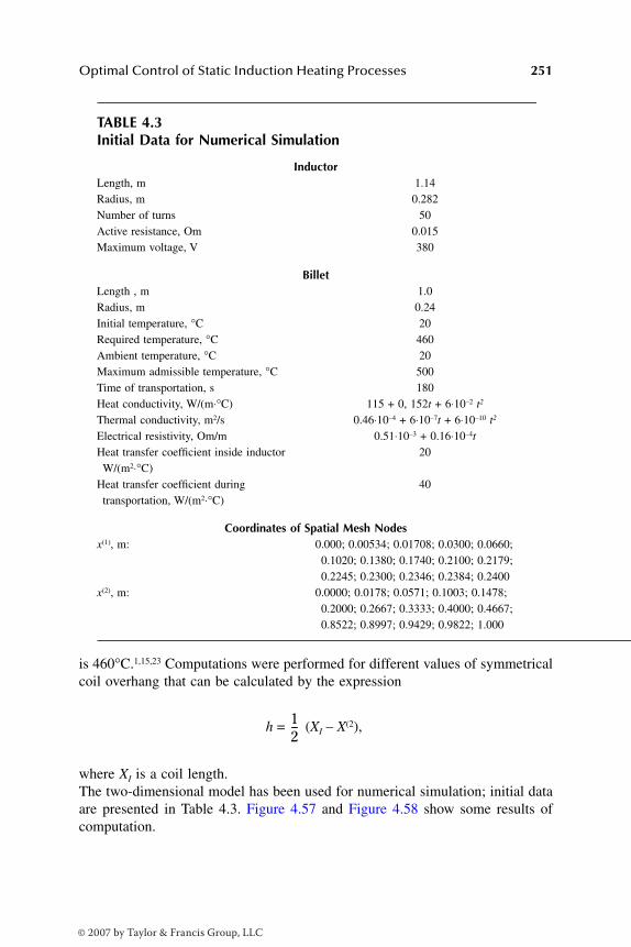
Optimal Control of Static Induction Heating Processes 251
is 460°C.1,15,23 Computations were performed for different values of symmetricalcoil overhang that can be calculated by the expression
h = (XI – X(2),
where XI is a coil length.The two-dimensional model has been used for numerical simulation; initial dataare presented in Table 4.3. Figure 4.57 and Figure 4.58 show some results ofcomputation.
TABLE 4.3Initial Data for Numerical Simulation
InductorLength, m 1.14Radius, m 0.282Number of turns 50Active resistance, Om 0.015Maximum voltage, V 380
BilletLength , m 1.0Radius, m 0.24Initial temperature, °C 20Required temperature, °C 460Ambient temperature, °C 20Maximum admissible temperature, °C 500Time of transportation, s 180Heat conductivity, W/(m⋅°C) 115 + 0, 152t + 6⋅10–2 t2
Thermal conductivity, m2/s 0.46⋅10–4 + 6⋅10–7t + 6⋅10–10 t2
Electrical resistivity, Om/m 0.51⋅10–3 + 0.16⋅10–4tHeat transfer coefficient inside inductor W/(m2⋅°C)
20
Heat transfer coefficient during transportation, W/(m2⋅°C)
40
Coordinates of Spatial Mesh Nodes x(1), m: 0.000; 0.00534; 0.01708; 0.0300; 0.0660;
0.1020; 0.1380; 0.1740; 0.2100; 0.2179; 0.2245; 0.2300; 0.2346; 0.2384; 0.2400
x(2), m: 0.0000; 0.0178; 0.0571; 0.1003; 0.1478; 0.2000; 0.2667; 0.3333; 0.4000; 0.4667; 0.8522; 0.8997; 0.9429; 0.9822; 1.000
12---
DK6039_C004.fm Page 251 Thursday, June 8, 2006 12:34 PM
© 2007 by Taylor & Francis Group, LLC
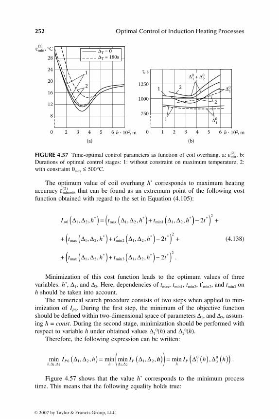
252 Optimal Control of Induction Heating Processes
The optimum value of coil overhang h* corresponds to maximum heatingaccuracy that can be found as an extremum point of the following costfunction obtained with regard to the set in Equation (4.105):
(4.138)
Minimization of this cost function leads to the optimum values of threevariables: h*, ∆1, and ∆2. Here, dependencies of tmax, tmin1, tmin2, t′min2, and tmin3 onh should be taken into account.
The numerical search procedure consists of two steps when applied to min-imization of IP6. During the first step, the minimum of the objective functionshould be defined within two-dimensional space of parameters ∆1, and ∆2, assum-ing h = const. During the second stage, minimization should be performed withrespect to variable h under obtained values ∆1
0(h) and ∆20(h).
Therefore, the following expression can be written:
.
Figure 4.57 shows that the value h* corresponds to the minimum processtime. This means that the following equality holds true:
FIGURE 4.57 Time-optimal control parameters as function of coil overhang. a: . b:Durations of optimal control stages: 1: without constraint on maximum temperature; 2:with constraint θmax ≤ 500°C.
1
2
0 2 3
(a) (b)
4 5 6 h ⋅ 102, m h ⋅ 102, m
8
16
12
20
24
28
1 2
1
2
0 2 3 4 51 6
750
1000
1250
τ, s
∆01
∆01 + ∆0
2
∆01
∆Τ = 0∆Τ = 180s
εmin , °C(2)
εmin( )2
εminmin( )2
I h t h t hp6 1 2 1 2 1 1 2∆ ∆ ∆ ∆ ∆ ∆, , , , , ,*max
*min
*( ) = ( ) + ( )) −( ) +
+ ( ) + ′ ( ) −
22
1 2 2 1 2
t
t h t h
*
max*
min*, , , ,∆ ∆ ∆ ∆ 22
2
2
1 2 3 1 2
t
t h t h t
*
max*
min* *, , , ,
( ) +
+ ( ) + ( ) −∆ ∆ ∆ ∆(( )2.
min , , min min , ,, , ,h
Ph
PI h I∆ ∆ ∆ ∆
∆ ∆ ∆ ∆1 2 1 2
6 1 2 1 2( ) = hh I h hh
P( )( ) = ( ) ( )( )min ,∆ ∆10 0
2
DK6039_C004.fm Page 252 Thursday, June 8, 2006 12:34 PM
© 2007 by Taylor & Francis Group, LLC
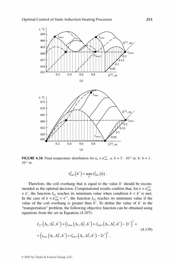
Optimal Control of Static Induction Heating Processes 253
.
Therefore, the coil overhang that is equal to the value h* should be recom-mended as the optimal decision. Computational results confirm that, for ε == ε*, the function IP1 reaches its minimum value when condition h < h* is met.In the case of ε = = ε**, the function IP2 reaches its minimum value if thevalue of the coil overhang is greater than h*. To define the value of h* in the“transportation” problem, the following objective function can be obtained usingequations from the set in Equation (4.107):
(4.139)
FIGURE 4.58 Final temperature distribution for ε0 = . a: h = 5 ⋅ 10–2 m. b: h = 1 ⋅10–2 m.
t, °C
t, °C
X(2), m
X(2), m
X(1), m
X(1), m
0.2 0.4 0.8 0.6
(a)
(a)
0.05
0.1
0.15
0.2
tmin3
tmin2
tγmin2
tmax tmax
tmax
460
454
451
457
463
466
469
0.2 0.4 0.8 0.6
0.05
0.1
0.15
0.2 460
450
445
455
465
470
475
tmin1
εmin( )2
τ τmin*
minmin0 0h hh
( ) = ( )
εmin( )2
εmin( )2
I h t h tp T T T7 10
10
2 10∆ ∆ ∆ ∆ ∆ ∆, , , , ,*
max*
min( ) = ( ) + ′ ,,
, , ,
* *
max*
min
h t
t h tT T
( ) −( ) +
+ ( ) + ′
22
10
3 10∆ ∆ ∆ ∆ ,, .* *h t( ) −( )2
2
DK6039_C004.fm Page 253 Thursday, June 8, 2006 12:34 PM
© 2007 by Taylor & Francis Group, LLC

254 Optimal Control of Induction Heating Processes
Therefore, the proper choice of coil overhang can be considered as an effectiveway to control (spatial control) induction heating processes.
REFERENCES
1. Rapoport, E.Ya., Optimization of Induction Heating of Metal, Metallurgy, Mos-cow, 1993.
2. Rapoport, E.Ya., Optimization problems for induction heating of metals prior topressure processing, Physica i Chimija obrabotki materialov, Moscow, 3, 54, 1984.
3. Rapoport, E.Ya., Optimal modes of metals heating with technological constraints,Izvestija Vuzov, Chernaya Metallurgija, 2, 101, 1986.
4. Rapoport, E.Ya., Optimization of Induction Heating Processes, Proc. 40 Int.Wis-senschaftliches Kolloquium, Technische Universitaet Ilmenau, Thueringen, 1995,48.
5. Rapoport, E.Ya., Parametric optimization of coupled electromagnetic and temper-ature fields in induction heating, Proc. Int. Symp. Electromagn. Fields Electr. Eng.(ISEF’95), Thessaloniki, 1995, 319.
6. Jaitskov, S.A., Accelerated Isothermal Induction Heating of Metals in Forging,Mashgiz, Moscow, 1962.
7. Pavlov, N.A., Engineering Thermal Design of Induction Heaters, Energia, Mos-cow, 1978.
8. Rapoport, E.Ya., About one problem of optimal control of metals heating, Izvestijavuzov, Energetica, 3, 67, 1980.
9. Germejer, Yu.B., Introduction in Theory of Operations Analysis, Nauka, Moscow,1971.
10. Rapoport, E.Ya., Robust parametric optimization of dynamic systems under con-dition of limited uncertainty, Avtomatika i telemehanika, 3, 86, 1995.
11. Butkovskij, A.G., Malyj, S.A., and Andreev, Yu.N., Optimal Control of MetalsHeating, Metallurgy, Moscow, 1972.
12. Butkovskij, A.G., Malyj, S.A., and Andreev, Yu.N., Control of Metals Heating,Metallurgy, Moscow, 1981.
13. Bryson, A. and Yu-Chi Ho, J.R., Applied Optimal Control: Optimization, Estima-tion and Control, Waltham, MA, Toronto, London, 1969.
14. Rapoport, E.Ya., Method of optimal process computation for heat treatment ofmaterials, Physica i Chimija obrabotki materialov, 5, 5, 1987.
15. Nemkov, V.S. and Demidovich, V.B., Theory and Computation of Induction Heat-ing Installations, Energoatomizdat, St. Petersburg, 1988.
16. Zimin, L.S., Features of heating of rectangular shape bodies, Primenenie tokovvysokoj chastoty v Electrotermii, Mashinostroenie, St. Petersburg, 25, 1973.
17. Rapoport, E.Ya. and Zimin, L.S., Optimal control of slabs induction heating beforerolling, Physica i chimija obrabotki materialov, 3, 21, 1986.
18. Rapoport, E.Ya., Optimal control in two-dimensional problems of heat transfer,Izvestija AN SSSR. Energetica i transport, 6, 102, 1984.
19. Rapoport, E.Ya., Optimization of two-dimensional processes of nonstationary heattransfer, Izvestija AN SSSR. Energetica i transport, 1, 86, 1985.
DK6039_C004.fm Page 254 Thursday, June 8, 2006 12:34 PM
© 2007 by Taylor & Francis Group, LLC
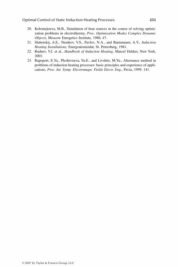
Optimal Control of Static Induction Heating Processes 255
20. Kolomejtseva, M.B., Simulation of heat sources in the course of solving optimi-zation problems in electrothermy, Proc. Optimization Modes Complex DynamicObjects, Moscow Energetics Institute, 1980, 47.
21. Sluhotskij, A.E., Nemkov, V.S., Pavlov, N.A., and Bamunauer, A.V., InductionHeating Installations, Energoatomizdat, St. Petersburg, 1981.
22. Rudnev, V.I. et al., Handbook of Induction Heating, Marcel Dekker, New York,2003.
23. Rapoport, E.Ya., Pleshivtseva, Yu.E., and Livshits, M.Yu., Alternance method inproblems of induction heating processes: basic principles and experience of appli-cations, Proc. Int. Symp. Electromagn. Fields Electr. Eng., Pavia, 1999, 141.
DK6039_C004.fm Page 255 Thursday, June 8, 2006 12:34 PM
© 2007 by Taylor & Francis Group, LLC
257
5
Optimal Control of Progressive and Continuous Induction Heating Processes
The majority of induction billet heaters utilize a heating mode where billets aremoved through a heater. This chapter will provide a study of the wide range ofoptimal control problems for progressive and continuous induction heating modes(Section 1.3). The
progressive heating
mode occurs when two or more heatedworkpieces (e.g., billets) are moved (via pusher, indexing mechanism, walkingbeam, etc.) through a single coil or inline multicoil induction heater. Therefore,components are sequentially heated (in a progressive manner) at certain prede-termined heating stages inside the heater. With the
continuous heating
mode, theworkpiece is moved in a continuous motion through one or more inline inductionheating coils. This heating mode is commonly used when it is necessary to heatlong components such as bars, slabs, strips, tubes, wires, blooms, and rods.
Progressive and continuous heaters are considered
at steady-state operationconditions
.
This chapter discusses the optimal control problems for continuous andprogressive heating modes based on a suggested parametric optimization method,taking into consideration the most typical real-life operating requirements.
The control inputs applied to continuous and progressive heating processesare quite different compared to those that were used in static heating. In contin-uous and progressive heating applications (see Section 2.4), control inputs includetime-invariant, but space-dependent control functions (spatial or distributed con-trol inputs). The spatial control function can be considered as a time-dependentoptimal control scanning along the heater length or as a set of constant parametersof an induction heating system. Obviously, space-dependent control inputs rep-resent design solutions employed at the stage of IHI design (see Section 2.4 andSection 2.8).
For progressive heating, these design solutions could also be complementedby cyclic periods of heating power variation in time, which allows performingoptimal process control algorithms during each process stage. This includesbetween successive unloading and loading of billets and billet transportationbetween different inline induction coils.
Basic methods of optimal control problem solution with respect to differentmathematical models will be presented as well. It will be shown that optimization
DK6039_C005.fm Page 257 Thursday, June 8, 2006 2:31 PM
© 2007 by Taylor & Francis Group, LLC
258
Optimal Control of Induction Heating Processes
results are in good qualitative agreement with results obtained earlier for staticheating.
5.1 OPTIMIZATION OF CONTINUOUS HEATERS AT STEADY-STATE OPERATING CONDITIONS
5.1.1 O
VERVIEW
OF
T
YPICAL
O
PTIMIZATION
P
ROBLEMS
AND
M
ETHODS
FOR
T
HEIR
S
OLUTION
Let us consider continuous induction heating installation where billets are movedend to end through a heater at constant speed
V
(Section 1.3). The fixed value of
V
corresponds to required throughput of the technological complex “inductionheater–hot working equipment.”
As shown earlier, the problem of providing the heating accuracy
ε
at the exitof inductor having the minimum length under given constraints can be consideredinstead of a general time-optimal control problem for static heating (see Section2.8). The general time-optimal problem is reduced to minimizing of the heaterlength when speed
V
of workpiece movement is prescribed
.
As was discussedearlier with respect to the basic mathematical model, the spatial distribution ofpower
u
*
(
y
/
V
) along the heater length can be considered as optimal control input.The time of static heating corresponds to the spatial coordinate along the inductor
in the case of continuous heating. Similarly to time-optimal control (Equation 2.27),optimal heat power distribution can be obtained as a stepwise function in the formof Equation (2.32). Bursts of power represent the maximum power of inline coilsthat may have different length and windings and/or can be individually fed fromdifferent power supplies. Therefore, an optimal heat power distribution can be imple-mented by using alternating inline coils with “heat ON” and “heat OFF” that repre-sent active and passive intervals of the lengths .
The shape of optimal control algorithm,
u
*
, is known, but the number,
N
, ofalternating inline coils and their lengths remain unknown. The problem of heaterlength optimization can be reduced to the problem of mathematical programmingin Equation (2.33).
After substitution of a variable (Equation 2.6), the optimal control function
u
*
(
ϕ
) in the time-optimal problem (Equation 2.34) coincides with function
u
*
(
y
/
V
)in the problem in Equation (2.33) that minimizes heater length. The basic one-dimensional mathematical model (Equation 1.27 through Equation 1.35) can beapplied in this case (see Section 2.8). Indeed, the optimal control
u
*
(
y
/
V
) can beproperly considered as a time-dependent power control
u
*
(
ϕ
) scanned along theheater length.
Therefore, after substitution (Equation 2.6), the power-control algorithm(Equation 2.32) for the problem in Equation (2.33) can be determined from thesolution of the problem in Equation (2.34). This solution was described in detailin Chapter 3 and Chapter 4. In this case, the maximum heating accuracy problem(Equation 2.37) for continuous heater of the given length has the same solutionas similar problems (Equation 2.35 and Equation 2.36) for static heating mode.
∆i i N*, ,= 1
DK6039_C005.fm Page 258 Thursday, June 8, 2006 2:31 PM
© 2007 by Taylor & Francis Group, LLC

Control of Progressive and Continuous Induction Heating Processes
259
The problems in Equation (2.35), Equation (2.36), and Equation (2.37) canbe reduced to the time-optimal problems, if the heater length does not exceedminimum length required for heating with utmost accuracy,
ε
inf
(Section 2.9.1).Only in rare cases, when the last condition is not satisfied, the problem forproviding maximum accuracy have an infinite solution set.
Therefore, if spatial heat source distribution is chosen as a control functionapplied to the mathematical model of a heating process (Equation 1.27 throughEquation 1.35), then the solution of the minimum-length problem for continuousinduction heating with required accuracy is known. This conclusion holds truefor the problem of obtaining the maximum heating accuracy with respect to acontinuous heater of the given length.
The basic model has been obtained under a number of simplified assumptions.In particular, this model describes a temperature field under assumption that aneffect of heat transfer in the axial direction by heat conduction is negligibly small(Section 2.2). To increase simulation accuracy further, two-dimensional heattransfer equations can be used.
In contrast to two-dimensional models of static heating (Section 4.5.1), con-tinuous heaters at steady-state operating conditions can be described by stationarytime-invariant equations for temperature distribution along the length and theradius of the billet.
In many cases, accurate simulation requires the use of more complicatedmathematical models. In particular, the inherently nonlinear nature of the induc-tion heating process of ferromagnetic billets implies nonlinearity of the model.This model takes into account temperature dependencies of all electromagneticand thermal properties of the heated material.
It can be shown
1
that the previously described optimal control method canbe extended to more complicated models of induction heating processes. Similarlyto the time-optimal problem for static heating, optimal spatial distribution of heatpower can be written in the form of Equation (2.32). All basic properties (Equation3.39 and Equation 3.40) of final temperature distribution within the billet at theinductor exit remain unchanged regardless of complicating factors.
Similarly to the case of the one-dimensional model (Section 4.1), theseconclusions are valid for optimal control problems taking into considerationtechnological constraints. This means that the form of optimal control
u
*
(
y
/
V
)becomes more complicated than the control input (Equation 2.32)
,
(similarly tothe general time-optimal problem).
As experience of computation shows,
1
the shape of the final (i.e., at the inductorexit) temperature
profile along the radius and appropriate sets of equations, obtainedearlier for the time-optimal problem, remain the same
.
Only expressions thatdescribe temperature distribution along the radius/thickness of the heated workpieceare varied.
These expressions should be written in an explicit form as functions ofspatial coordinates and optimal control parameters. They can be obtained aftersolving heat transfer equations using analytical or numerical methods.
However, mathematical models for static and continuous heating processesare not the same. It is still possible to accept as a physically based approach that
DK6039_C005.fm Page 259 Thursday, June 8, 2006 2:31 PM
© 2007 by Taylor & Francis Group, LLC

260
Optimal Control of Induction Heating Processes
the optimal algorithm of heat power control for continuous heaters can be con-sidered as a spatial scanning of time-dependent optimal power control for staticheaters. The dependences of these algorithms on axial coordinate and time haveidentical forms (Equation 2.32 and Equation 2.27), but their parameters can benoticeably different.
The voltages
U
1
,
U
2
, …,
U
N
for
N
coils of an induction heater can beconsidered as spatial control inputs for multicoil inductor design (Section 2.4 andSection 2.9); therefore, they can be treated as unknown parameters .The number of sections,
N
, and their lengths are defined by the given IHI design.In this case an optimal problem can be formulated as the problem (Equation 2.38)of maximum heating accuracy. Refined models should include different factorsincluding gaps between coils.
Experience in solving similar problems
1–5
confirms that optimal final temper-ature distribution within a billet cross-section and computational sets of equationsremain similar to the general time-optimal problem, regardless of the complexityof mathematical models. The most important conclusion is that the alternancemethod can be used in this case if the temperature distribution can be obtainedas a function of spatial coordinates and voltages .
However, the choice of coil voltages as spatial control inputs leads to someunique features.
4,5
The set of optimal voltages for
N
coils of given lengths allowsone to realize optimal heat power distribution along the multicoil continuousheater. This distribution represents time-dependent heat power control scanningalong the length of the induction heater. Therefore, the heating cycle has presetnumber and durations of process stages defined by the given IHI design. Tem-perature distribution can be affected through a set of control inputs by choosingthe values,
U
i
, for each inductor coil.The opposite situation occurs when the heat power distribution,
u
(
y
/
V
), ischosen as a control input. According to Equation (2.32), the optimal control
u
*
takes only fixed limit values, and one can modify temperature distribution withinthe billet by choosing the number and durations of alternating heating/soakingstages.
From the preceding discussion, it follows that optimal heat power controlutilizing coil voltages provides multiposition control (Figure 2.11); the val-ues differ from their admissible limit values. The optimal controlfunction (Equation 2.32) represents on–off control that takes only two extremevalues.
The consideration of optimal voltages (
U
10
,
U
20
, …,
U
N
0
) as parameters forvarying heat power distribution with time allows transforming (in terms of qual-itative characteristics) a maximum accuracy problem (Equation 2.38) into anequivalent time-optimal problem. The “inverse” transformation from time-opti-mal problem to the problem on maximum accuracy has been explored in Section2.9.1.
Let us assume that the condition in Equation (3.3) remains valid for theequivalent time-optimal problem. This condition links required accuracy
ε
withnumber of required optimal control intervals where voltage is constant. In this
∆i i N, ,= 1
U i Ni, ,= 1
U i Ni0 1, ,=
DK6039_C005.fm Page 260 Thursday, June 8, 2006 2:31 PM
© 2007 by Taylor & Francis Group, LLC
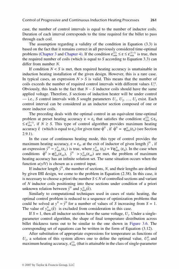
Control of Progressive and Continuous Induction Heating Processes
261
case, the number of control intervals is equal to the number of inductor coils.Duration of each interval corresponds to the time required for the billet to passthrough each coil.
The assumption regarding a validity of the condition in Equation (3.3) isbased on the fact that it remains correct in all previously considered time-optimalproblems (Chapter 3 and Chapter 4). If the condition
≤
ε
≤
is true, thenthe required number of coils (which is equal to
S
according to Equation 3.3) candiffer from number
N
.If condition
N
<
S
is met, then required heating accuracy is unattainable ininduction heating installation of the given design. However, this is a rare case.In typical cases, an expression
N
>
S
is valid. This means that the number ofcoils exceeds the number of required control intervals with different values
U
i
0
.Obviously, this leads to the fact that
N
–
S
inductor coils should have the sameapplied voltage. Therefore,
S
sections of induction heater will be under control— i.e.,
S
control intervals with
S
sought parameters
U
1
,
U
2
, …,
U
S
exist. Eachcontrol interval can be considered as an inductor section composed of one ormore inductor coils.
The preceding deals with the optimal control in an equivalent time-optimalproblem at preset heating accuracy
ε
=
ε
0
that satisfies the condition:
≤ ε
0
≤
, if
N
≥
S
. This type of control algorithm provides maximum heatingaccuracy (which is equal to
ε
0
) for given time , if =
0
ϕ
min
(
ε
0
) (see Section2.9.1).
In the case of continuous heating mode, this type of control provides themaximum heating accuracy,
ε
=
ε
0
, at the exit of inductor of given length , ifan expression is true, where
y
min0
(
ε
0
) =
V
ϕ
min0
(
ε
0
). In the case whenconditions >
0ϕmin(εinf), > 0ymin(εinf) are met, the problem of maximumheating accuracy has an infinite solution set. The same situation occurs when thefunction u(y/V) is chosen as a control input.
If inductor length , the number of sections, N, and their lengths are definedby given IHI design, we come to the problem in Equation (2.38). In this case, itis necessary to choose a priori the number S ≤ N of controlled sections and variantof N inductor coils positioning into these sections under condition of a prioriunknown relation between and 0ymin(ε).˜
Similarly to computational techniques used in cases of static heating, theoptimal control problem is reduced to a sequence of optimization problems thatcould be solved at for a number of values of S increasing from S = 1.The value of is excluded from consideration in this case.
If S = 1, then all inductor sections have the same voltage, U1. Under a single-parameter control algorithm, the shape of final temperature distribution acrossbillet thickness turns out to be similar to the one shown in Figure 3.6. Thecorresponding set of equations can be written in the form of Equation (3.12).
After substitution of appropriate expressions for temperature as functions ofU1, a solution of this system allows one to define the optimal value, U1,
0 andmaximum heating accuracy, (that is attainable in the class of single-parameter
εmin( )S εmin
( )S−1
εmin( )S
εmin( )S−1
ε ϕ0 ϕ0
y0
y y0 00= min ( )ε
ϕ0 y0
y0
y0
y y0 0= ymin ( )0 ε
εmin( )1
DK6039_C005.fm Page 261 Thursday, June 8, 2006 2:31 PM
© 2007 by Taylor & Francis Group, LLC
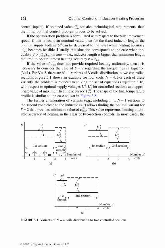
262 Optimal Control of Induction Heating Processes
control inputs). If obtained value satisfies technological requirements, thenthe initial optimal control problem proves to be solved.
If the optimization problem is formulated with respect to the billet movementspeed, V, that is less than nominal value, then for the fixed inductor length, theoptimal supply voltage U1
0 can be decreased to the level when heating accuracybecomes feasible. Usually, this situation corresponds to the case when ine-
quality y0 > 0ymin(εinf) is true — i.e., inductor length is bigger than minimum lengthrequired to obtain utmost heating accuracy ε = εinf.
If the value of does not provide required heating uniformity, then it isnecessary to consider the case of S = 2 regarding the inequalities in Equation(3.41). For N > 2, there are N – 1 variants of N coils’ distribution to two controlledsections. Figure 5.1 shows an example for four coils, N = 4. For each of thesevariants, the problem is reduced to solving the set of equations (Equation 3.16)with respect to optimal supply voltages U1,
0 U20 for controlled sections and appro-
priate value of maximum heating accuracy . The shape of the final temperatureprofile is similar to the case shown in Figure 3.8.
The further enumeration of variants (e.g., including 1 … N – 1 sections tothe second zone close to the inductor exit) allows finding the optimal variant forS = 2 that provides minimum value of . This value represents limiting attain-able accuracy of heating in the class of two-section controls. In most cases, the
FIGURE 5.1 Variants of N = 4 coils distribution to two controlled sections.
εmin( )1
εmin( )1
εmin( )1
εmin( )2
εmin( )2
1 2 3 4
I II III IV
1 2 3 4
1 2 3 4
1st section 2nd
section
1st section 2nd section
1st
section
2nd section
Number of
coils
Number of
coils
Number of
coils
(b)
(c)
(a)
DK6039_C005.fm Page 262 Thursday, June 8, 2006 2:31 PM
© 2007 by Taylor & Francis Group, LLC

Control of Progressive and Continuous Induction Heating Processes 263
obtained value, , satisfies technological requirements, and the initial optimalcontrol problem proves to be solved.
Based on common sense, it is possible to assume that, for values of closeto ymin
0 ( ), “scanning in time” optimal programs for varying feeding voltagesalong inductor length approximate to the time-optimal heat power control. There-fore, for such values , the feeding voltage U1
0 of the first section usually exceedsthe value U2,
0 similarly to two-stage control (Equation 2.27) (Figure 5.1, solidcurves).
As the value of becomes higher than ymin0 ( ), the relation between 0U1
and U20 can be varified in the opposite way (Figure 5.1, dashed curves). If the
heating accuracy for S = 2 is not acceptable, then it is necessary to consider thecase of using three controlled sections (S = 3); further searching for optimalvalues U1,
0 U2,0 and U3
0 can be done in a similar manner. It should be kept in mindthat, under condition N > S, the number of variants of controlled coils positioninggrows rapidly in comparison with the case of S = 2. Similarly to static heatingmode, the heating accuracy attainable for S = 3 coincides with the value ofutmost accuracy εinf (Section 3.3 and Section 3.6).
General considerations discussed here can be applied to different optimizationproblems subject to additional complicating factors (Chapter 4), as has been donefor static heating optimization. Typical optimization problems will be furtherdiscussed for a variety of particular control inputs. The optimization problemwith respect to continuous heating application models will be discussed later.
5.1.2 DESIGN OF MINIMUM LENGTH INDUCTOR
Let us consider the optimal design problem that minimizes heater length whenspeed V of workpiece movement through an induction heater is constant and arequired heating accuracy should be obtained at the inductor exit.1 Spatial distri-bution of power u*(y/V) along the heater length can be chosen as control inputconstrained by Equation (2.8). This problem can be formulated as the mathemat-ical programming problem (Equation 2.33).
A more precise model may be used for calculation of temperature distribution,θ(l,y), taking into account the heat transfer by conduction along the radius (coor-dinate l) and the length (coordinate y) of the heated cylindrical billet. Using thesystem of relative units, the temperature distribution, θ(l,y), within the billet (thatmoves through the inductor at constant speed V = const) can be described by thelinear two-dimensional stationary heat transfer equation of the following form1:
(5.1)
with the boundary conditions:
εmin( )2
y0
εmin( )2
y0
y0 εmin( )2
εmin( )S
∂∂
+ ∂∂
+ ∂∂
− ∂2
22
2
2
1θ θ β θ β θ( , ) ( , ) ( , ) (l y
l l
l y
l
l y
yV
ll y
yW l y
l y y
d
, )( , , ) ,
; ;
∂+ =
< < < <
ξ 0
0 1 0 0
DK6039_C005.fm Page 263 Thursday, June 8, 2006 2:31 PM
© 2007 by Taylor & Francis Group, LLC
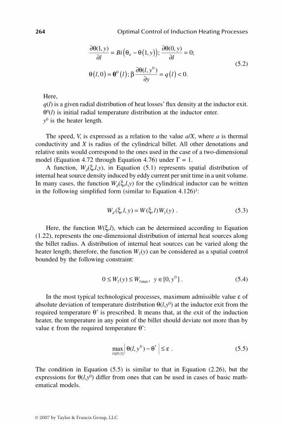
264 Optimal Control of Induction Heating Processes
(5.2)
Here,q(l) is a given radial distribution of heat losses’ flux density at the inductor exit.θ0(l) is initial radial temperature distribution at the inductor enter.y0 is the heater length.
The speed, V, is expressed as a relation to the value a/X, where a is thermalconductivity and X is radius of the cylindrical billet. All other denotations andrelative units would correspond to the ones used in the case of a two-dimensionalmodel (Equation 4.72 through Equation 4.76) under Γ = 1.
A function, Wd(ξ,l,y), in Equation (5.1) represents spatial distribution ofinternal heat source density induced by eddy current per unit time in a unit volume.In many cases, the function Wd(ξ,l,y) for the cylindrical inductor can be writtenin the following simplified form (similar to Equation 4.126)1:
. (5.3)
Here, the function W(ξ,l), which can be determined according to Equation(1.22), represents the one-dimensional distribution of internal heat sources alongthe billet radius. A distribution of internal heat sources can be varied along theheater length; therefore, the function W1(y) can be considered as a spatial controlbounded by the following constraint:
. (5.4)
In the most typical technological processes, maximum admissible value ε ofabsolute deviation of temperature distribution θ(l,y0) at the inductor exit from therequired temperature θ* is prescribed. It means that, at the exit of the inductionheater, the temperature in any point of the billet should deviate not more than byvalue ε from the required temperature θ*:
. (5.5)
The condition in Equation (5.5) is similar to that in Equation (2.26), but theexpressions for θ(l,y0) differ from ones that can be used in cases of basic math-ematical models.
∂∂
= − ( )( ) ∂∂
=
( ) =
θ θ θ θ
θ
( , ), ;
( , );
,
11
00
0
y
lBi y
y
l
l
a
θθ β θ00
0ll y
yq l( ) ∂
∂= ( ) <;
( , ).
W l y W l W yd ( , , ) ( , ) ( )ξ ξ= 1
0 01 10≤ ≤ ∈W y W y y( ) , [ , ]max
max ( , )[ , ]
*
ll y
∈− ≤
0 1
0θ θ ε
DK6039_C005.fm Page 264 Thursday, June 8, 2006 2:31 PM
© 2007 by Taylor & Francis Group, LLC

Control of Progressive and Continuous Induction Heating Processes 265
Let us formulate the optimal control problem with respect to a continuousheater at steady-state operating conditions as follows. It is necessary to selectcontrol function W1
*(y) restrained by Equation (5.4) that provides steering billets’initial temperature distribution to desired temperature θ* = const with prescribedaccuracy ε (according to Equation 5.5), while minimizing inductor length y0.
It can be proved1 that optimal heat power distribution W1*(y) can be repre-
sented as a stepwise function in the form of Equation (2.32) (Figure 2.10):
. (5.6)
This means that the optimal design solution represents a heater consisting ofalternating inline sections with heat ON and heat OFF power intervals (activeand passive zones).
Therefore, the solution of the problem that minimizes length of continuousheater and provides required accuracy is known, but the number, N, of alternatinginline sections and their lengths ∆i, i = remain unknown. Similarly toEquation (2.33), the problem that minimizes the length of the induction heatercan be reduced to the problem of mathematical programming:
(5.7)
(5.8)
The alternance method can be successfully applied to a wide variety ofspecific optimization problems of the type in Equation (5.7) and Equation (5.8).In this case, previously described universal properties of final temperature distri-bution, sets of appropriate equations, and computational techniques remainunchanged as applied to time-optimal problems with respect to static heating.
It is important to note at this point that the expressions in governing sets thathave been used in the case of optimization of static heating describe the temper-ature distribution at the end of the heating cycle. In the case of continuous heatingmode, these expressions represent temperature distribution within billet cross-section at the inductor exit under y = y0.
In contrast to the problem in Equation (2.33), there is a specific dependenceof temperature θ(l,y0,∆) as a function of spatial coordinates and control para-meters. This dependence should be obtained after solving two-dimensional heattransfer Equation (5.1) and Equation (5.2).
Let us accept that y0 = 1 with respect to relative units. Assuming that initialtemperature distribution at the inductor inlet can be considered as uniform along
W yW
y y y j Njj j1
1 112
1 1 1* max( ) ( ) , , , ,= + − < < =+− yy yN = 0
1 N,
I
l y
i
i
N
l
( ) min;
( ) max ( , , )[ , ]
∆ ∆
Φ ∆ ∆
∆= →
= −
=
∈
∑1
0 1
0θ θθ ε* .≤
DK6039_C005.fm Page 265 Thursday, June 8, 2006 2:31 PM
© 2007 by Taylor & Francis Group, LLC
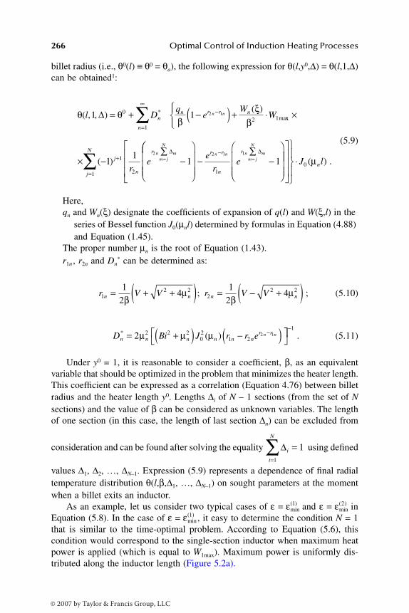
266 Optimal Control of Induction Heating Processes
billet radius (i.e., θ0(l) ≡ θ0 = θa), the following expression for θ(l,y0,∆) = θ(l,1,∆)can be obtained1:
(5.9)
Here,qn and Wn(ξ) designate the coefficients of expansion of q(l) and W(ξ,l) in the
series of Bessel function J0(µnl) determined by formulas in Equation (4.88) and Equation (1.45).
The proper number µn is the root of Equation (1.43).r1n , r2n and Dn
* can be determined as:
(5.10)
. (5.11)
Under y0 = 1, it is reasonable to consider a coefficient, β, as an equivalentvariable that should be optimized in the problem that minimizes the heater length.This coefficient can be expressed as a correlation (Equation 4.76) between billetradius and the heater length y0. Lengths ∆i of N – 1 sections (from the set of Nsections) and the value of β can be considered as unknown variables. The lengthof one section (in this case, the length of last section ∆n) can be excluded from
consideration and can be found after solving the equality using defined
values ∆1, ∆2, …, ∆N–1. Expression (5.9) represents a dependence of final radialtemperature distribution θ(l,β,∆1, …, ∆N–1) on sought parameters at the momentwhen a billet exits an inductor.
As an example, let us consider two typical cases of ε = and ε = inEquation (5.8). In the case of ε = , it easy to determine the condition N = 1that is similar to the time-optimal problem. According to Equation (5.6), thiscondition would correspond to the single-section inductor when maximum heatpower is applied (which is equal to W1max). Maximum power is uniformly dis-tributed along the inductor length (Figure 5.2a).
θ θβ
ξβ
( , , )( )*
mal Dq
eW
Wnn r r nn n1 10
2 12 1∆ = + −( ) + ⋅−
xx
( )
×
× −∑
−
=
∞
+
=
∑
∑ =
n
j
j
N
n
r
re
n mm j
N
1
1
1 2
11
12 ∆
−∑
−
−=e
re
r r
n
rn n n mm j
N
2 1 1
1
1∆
⋅ J ln0 ( ) .µ
r V V r V Vn n n n12 2
22 21
24
12
4= + +( ) = − +( )βµ
βµ; ;
D Bi J r r en n n n n nr rn n* ( )= +( ) −( )
−2 2 2 2
02
1 22 1µ µ µ
−1
∆i
i
N
==∑ 1
1
εmin( )1 εmin
( )2
εmin( )1
DK6039_C005.fm Page 266 Thursday, June 8, 2006 2:31 PM
© 2007 by Taylor & Francis Group, LLC
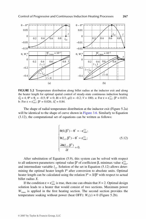
Control of Progressive and Continuous Induction Heating Processes 267
The shape of radial temperature distribution at the inductor exit (Figure 5.2a)will be identical to the shape of curve shown in Figure 3.6. Similarly to Equation(3.12), the computational set of equations can be written as follows:
(5.12)
After substitution of Equation (5.9), this system can be solved with respectto all unknown parameters: optimal value β0 of coefficient β, minimax value ,and intermediate variable le2. Solution of the set in Equation (5.12) allows deter-mining the optimal heater length Y0 after conversion to absolute units. Optimalheater length can be calculated using the relation Y0 = X/β0 with respect to actualbillet radius X.
If the condition ε = is true, then one can obtain that N = 2. Optimal designsolution leads to a heater that would consist of two sections. Maximum powerW1max is applied in the first heating section. The second section provides thetemperature soaking without power (heat OFF): W1(y) ≡ 0 (Figure 5.2b).
FIGURE 5.2 Temperature distribution along billet radius at the inductor exit and alongthe heater length for optimal spatial control of steady-state continuous induction heating(ξ = 4; θ0 = θa = –0.5; θ* = 0; Bi = 0.5; q(l) = –0.2; V = 100). a: For ε = ; β0 = 0.031.b: For ε = ; β0 = 0.026; ∆1
0 = 0.84.
0
θ − θ∗ θ − θ∗
θ, W1∗ θ, W
1∗
0.05
−0.05
−0.10
0.4 0.8 le2
le2
0.2 0.6
0
−0.2
−0.4
0.4 0.8 y
(a) (b)
0.2 0.6 l = 1
l = 0
l = le2
l = 1
l = 0
l = le2
0 y
−0.2
−0.4
0.4 0.8 0.2 0.6
0
0.01
−0.01
−0.02
0.4 0.8 0.2 0.6
l
W1 max
× 10−1 W1 max
× 10−1
l
εmin( )1
εmin( )2
θ β θ ε
θ β θ ε
θ
( , ) ;
( , ) ;
*min( )
*min( )
0 0 1
20 1
− = −
− =
∂
le
(( , ).
l
le2
0
0β
∂=
εmin( )1
εmin( )2
DK6039_C005.fm Page 267 Thursday, June 8, 2006 2:31 PM
© 2007 by Taylor & Francis Group, LLC
268 Optimal Control of Induction Heating Processes
In the case of ε = εmin(2), the set of equations can be written in the form of
Equation (3.16) as:
(5.13)
After substitution of Equation (5.9), this set can be solved with respect to optimalvalue β0, optimal length of the first section ∆1
0 (using relative/dimensionless units),minimax value , and coordinate le2.
Obtained value β0 allows determining the optimal heater length Y0. Optimallengths of the first and second sections can be calculated as 0∆1Y0 and (1 – 0∆1)Y0,respectively. As a matter of fact, the second section of the induction heater canbe considered as “thermostat,” where the heating is not required. The inductorlength will be equal to the length of the first section. The problem can be reducedto the problem that minimizes the total length of the induction heating installation.
Let us consider a transfer time as total time from the moment when the heatedworkpiece exits an induction heater until beginning of the hot working operation.In this case, the second section can be unnecessary because the temperature willbe equalized during transfer stage. This is the typical case when an expression,∆T
0 ≥ *∆T2, is valid and heating accuracy, , will be in agreement withrequirements. Here, the variables 0∆T, *∆T2 and make the same sense as wasdiscussed in Section 4.2. Time-optimal heat power control in a “transportationproblem” consists of a single control interval under u*(ϕ) ≡ Umax (Section 4.2).
Spatial scanning of time-dependent control leads to the simplest single-section design solution with uniform maximum heat power distribution along thelength of the induction heater. In contrast to the case of N = 1, the requireduniformity of temperature distribution cannot be provided at the inductor exit,but sufficient temperature equalization, which takes place during the transfer stageof optimal duration, ensures obtaining required uniformity.
Minimum value of can be obtained at ∆T0 = *∆T2. If the time of transpor-
tation can be varied, then the duration of transfer stage meets the condition 0∆T =∆T2
* and will be considered as an optimal design solution as well.If transfer stage ∆T
0 is taken into account, then the computational equationsset remains similar to the “transportation” time-optimal problem. According toEquation (4.40), this set keeps the form of Equation (5.13) at ∆T
0 = ∆T2* or can be
transformed into form of Equation (4.41) or Equation (4.42) if ∆T0 > *∆T2.
In the first case, the value ∆T2* would be defined after solving the set of
equations. Obviously, the appropriate expressions for θ(l,β,∆,∆T)0 will be changed
θ β θ ε
θ β θ ε
( , , ) ;
( , , )
*min( )
*m
0 010 2
20
10
∆
∆
− = −
− =le iin( )
*min( )
;
( , , ) ;
( , ,
2
010 2
20
1
1θ β θ ε
θ β
∆
∆
− = −
∂ le00
0)
.∂
=
l
εmin( )2
ε ε= min( )2
εmin( )2
εmin( )2
DK6039_C005.fm Page 268 Thursday, June 8, 2006 2:31 PM
© 2007 by Taylor & Francis Group, LLC

Control of Progressive and Continuous Induction Heating Processes 269
in comparison with Equation (5.9). These expressions can be found after solvingthe corresponding set of heat transfer equations with regard to different levels ofheat losses from the billet surface during heating stage and transfer stage (Section4.2).
Figure 5.2 presents some computational results of determining optimal pro-cess parameters for continuous induction heater. In the typical cases of ε =and ε = , the final temperature distribution can be calculated from Expression(5.9). As one can see, the optimal design solution leads to the temperaturedistribution along billet radius at the heater exit that is similar to temperaturedistribution at the end of time-optimal process (Figure 3.6 and Figure 3.8). Thetemperature distribution within any cross-section of the billet located inside theheater proves to be identical to the temperature distribution that would correspondto appropriate time of static heating.
Similarly to Section 4.1, the requirement on the temperature distributionduring heating can be imposed. According to such a requirement, during heatingstage the value of maximum temperature anywhere within the heated workpieceshould not exceed a certain admissible value θadm. Therefore, instead of Expres-sion (2.11), the temperature maximum constraint can be written as follows:
. (5.14)
As an example, let us consider an optimal heater design problem taking intoconsideration the condition θadm = θ*. This condition means that temperature atany point within the billet should not be higher than required temperature θ*. Inthis case, the condition ε > θadm – θ* = 0 holds true under given heating accuracyε > 0.
Similarly to optimization of static heating (Section 4.1), the utmost admissiblevalue of heating accuracy ε coincides with . Optimal heat power distributionalong the length of an induction heater can be considered as a time-dependentoptimal control (Equation 4.3) with scanning along the heater length. For N = 1,the optimal heat power distribution can be written as follows:
(5.15)
According to Equation (5.15), the heater consists of two sections. In the firstsection, which is yθ long, the maximum heating power W1max is applied. Thesecond section represents a holding chamber of temperature θmax at the level θadm
= θ* under heat power Wθ (y). Therefore, continuous induction heating installationprovides accelerated heating mode (Section 4.1). Obviously, the function Wθ (y)should be written in the form similar to Expression (4.13) with respect to time-dependent function uθ(ϕ).
εmin( )1
εmin( )2
θ θ θmax, [ , ]
max ( , )= ≤∈
l yl y
adm0 1
εmin( )1
W yW y y
W y y y y1
1
0
0* max( )
, ;
( ), .=
≤ <
< ≤
θ
θθ
DK6039_C005.fm Page 269 Thursday, June 8, 2006 2:31 PM
© 2007 by Taylor & Francis Group, LLC

270 Optimal Control of Induction Heating Processes
A time-dependent control of the heat power can serve as a good example ofthe control input that can be relatively simply realized in the static inductionheater. However, practically speaking, one can face certain problems in realizationof providing nonuniform coil power distribution along the length of the secondsection. Therefore, it is reasonable to use the piecewise constant approximation,WA
θ (y), of function W θ(y) that can be relatively simply realized by providing aconstant heat power W (k), k = 1, 2, …, χ, χ ≥ 1 within each of χ inductor sections(Figure 5.3):
(5.16)
Under given number χ ≥ 1, the variables yk denote the bound point’s coordi-nates for heater sections. The powers W(k) and coordinates yk can be consideredas approximation parameters. If the temperature distribution as a function ofapproximation parameters is known, these parameters can be defined numericallyusing condition of minimum deviation of θmax from θadm at points within interval[yθ,y0]. Similarly to Equation (4.12), the coordinates (lmax,yθ) of the point at whichthe temperature θmax reaches an admissible value θadm can be found by consideringthe equalities:
. (5.17)
The temperature θ(lmax,yθ) should be found after solving Equation (5.1) andEquation (5.2) with substitution of control input in the form of Equation (5.15)and Equation (5.16). If we allow for relative/dimensionless units of length y0 =1, then instead of Equation (5.9) and after replacing y0 by coefficient β, thissolution can be written as follows1:
FIGURE 5.3 Piecewise constant approximation of optimal heat power distribution alongthe heater length.
W1∗(y)
W1 max
W (2)
W (1)
yθ y1 y2 y0 y
W (3)
~ ~
W y W y y y k
y y
Ak
k kθ
θ
χ( ) , ( , ), , ,( )= = ∈ =
=
−const
1 1
00 10< < < = y y y... .χ
θ θ θ θθ
θ( , ) ;( , )
max* maxl y
l y
ladm= = ∂∂
= 0
DK6039_C005.fm Page 270 Thursday, June 8, 2006 2:31 PM
© 2007 by Taylor & Francis Group, LLC
Control of Progressive and Continuous Induction Heating Processes 271
(5.18)
In the case of ε = (under defined values of yθ and WAθ (y)), the optimal
control input (Equation 5.15) has a single unknown parameter, β, that allowsdetermining the optimal heater length.
Similarly to Equation (4.24), the following computational set can be obtainedinstead of Equation (5.12):
(5.19)
After substitution of Equation (5.18), this set should be solved with respect tounknown variables β0 and .
However, it is impossible to find *W1(y) and coordinates lmax and yθ after separatesolving of appropriate equations sets because the output θ(l,y) from a heating processis obtained in response to applied input W1
*(y) varying on the interval (yθ,y0). Thismeans that, in contrast to static heating optimization, all unknown variables lmax, yθ,β0, and for each given set of values can be found by combinedsolution of sets of Equation (5.17) and Equation (5.19).
The values of W(k) and yk can be found by minimizing deviation of θmax fromθadm at the last stage of a solution of the discussed optimal control problem.
Figure 5.4 shows the computational results for optimal mode of continuousaccelerated heating that provides a holding of temperature θmax at the level θadm
= θ*. The computational procedure has been performed in the simplest case of χ= 1 and ε = = εinf, according to the previously described technique. All initialdata are the same as in the case shown in Figure 5.2.
Optimal temperature distribution along the radius of a cylindrical billet (Fig-ure 5.4a) at the inductor exit replicates in shape the temperature distribution atthe end of accelerated static heating (Figure 4.9). Temperature distribution alongthe heater length (Figure 5.4b) exhibits the acceptable accuracy of approximationof θmax to θadm = θ* within the interval [yθ, y0] in spite of the fact that uniformpower distribution WA
θ (y) = W(1) < W1max, y ∈ (yθ,y0) represents a crude approx-imation of the function Wθ(y).
θ β θβ
ξβ
( , )( )*l D
qe
Wen
n r r n rn n n= +
−( ) +−021 2 1 2
nn
n
r y
n
r y
re
ren n
=
∞
− −
∑ ×
× −( ) − −( )
1
1 2
11
111 2θ θ
⋅
+ −=
− −∑
W
Wr
e ek
k n
r y r yn k n k
1
1 1
1 1 1
max
( )
χ −− −( ) − −( )
− −1 2 2 1
1
2re e
n
r y r yn k n k
J ln0 ( ).µ
εmin( )1
θ β θ ε
θ β θ ε
( , ) ;
( , ) .
*min( )
*min( )
1
0
0 1
0 1
− = −
− = −
εmin( )1
εmin( )1 W y kk
k( ) , , , = 1 χ
εmin( )1
DK6039_C005.fm Page 271 Thursday, June 8, 2006 2:31 PM
© 2007 by Taylor & Francis Group, LLC

272 Optimal Control of Induction Heating Processes
Curves 1 through 3 in Figure 5.4 illustrate a process of searching for thevalue W (1) when minimizing deviation of θmax from θadm = θ*. Here, the optimalvalue of W (1) turns out to be equal to the value of 0.36 W1max (curve 2). Theobtained simple algorithm of spatial control can be relatively easily applied inengineering practice if each of the two sections of an induction heater has optimallength (depending on calculated value of yθ), and applied power will be equal tothe optimal value of W (1).
It is important to note that stepwise algorithms of optimal spatial control(Equation 5.6 or Equation 5.15, Equation 5.16) that have been found underidealized conditions of the relaxing constraint (Equation 5.4) cannot be accuratelyrealized using practical design solutions of continuous induction heating instal-lations. It is impossible to provide an absolutely uniform power distribution along
FIGURE 5.4 Optimal spatial control of continuous accelerated heating that provides aholding of temperature θmax at the admissible level (ξ = 4; θ0 = θa = –0.5; Bi = 0.5; q(l)= –0.2; V = 100; θadm = θ* = 0; ε = = εinf). a: Temperature distribution along billetradius under control in the form of Equation (5.16) for χ = 1 (1 – W(1)/W1max = 0.37; β0 =0.02; yθ = 0.52; 2 – W(1)/W1max = 0.36; β0 = 0.021; yθ = 0.54; 3 – W(1)/W1max = 0.3; β0 =0.024; yθ = 0.61). b: Distribution of heat power and temperature along the heater length(W(1)/W1max = 0.36; β0 = 0.021; yθ = 0.54; lmax = 0.93).
0
θ − θ∗
0.4 0.80.2
−0.02
−0.04
−0.06
1l
yθy
2
3
(a)
(b)
00.4 0.80.2 0.6
−0.5
−0.4
−0.3
−0.2
−0.1
l = lmax l = 1
l = 0
θ, W∗ × 10−1
W 1 max W (1)
εmin( )1
DK6039_C005.fm Page 272 Thursday, June 8, 2006 2:31 PM
© 2007 by Taylor & Francis Group, LLC
Control of Progressive and Continuous Induction Heating Processes 273
each section with stepwise power change from one section to another due to alongitudinal electromagnetic end effect and gaps between sections.2,6
Keep in mind that obtained results can be extended onto other optimal controlproblems, subject to complicating real-life constraints, by using coil voltagesapplied to controlled sections as control inputs. Moreover, obtained results exhibitquantitative and qualitative properties of optimal spatial control and deal withestimation of a maximum of capability of an induction heater. This can be veryhelpful in order to have a rough idea with regard to number of sections, powerlevels, and required shop floor space.
5.1.3 OPTIMIZATION OF THE CONTINUOUS HEATING OF FERROMAGNETIC MATERIALS
The continuous induction machinery for heating ferromagnetic materials is widelyused in industry. This process is governed by complex nonlinear equations. Thenonlinear nature of magnetic permeability as a function of temperature is respon-sible for the presence of ferromagnetic and paramagnetic phases of heatedmaterial. The ferromagnetic phase takes place at temperatures below the Curiepoint. The paramagnetic phase takes place if temperature of a heated workpieceexceeds the Curie temperature.
Transition between these phases leads to significant changes in intensity andspatial distribution of internal heat power during the induction heating process.Also, magnetic permeability and other physical properties make a marked effecton temperature distribution of heated workpieces. It is imperative to keep in mindthat electrical resistivity, thermal conductivity, and specific heat are also functionsof temperature (Section 4.6.2).
The two-dimensional equation (Equation 5.20) properly describes steady-state temperature distribution of the heated cylindrical billet using a continuousinduction heater1:
(5.20)
with the boundary conditions:
. (5.21)
Equation (5.20) and Equation (5.21) describe a temperature field duringsteady-state continuous heating under assumption that an effect of heat transfer
∂∂
+ ∂∂
− ∂∂
+2
2 11θ θ β θ α( , ) ( , )
( )( , )
( )l y
l l
l y
ly
l y
yy WW l y W y
l y y
d ( , ) ( ) ;
; ;
1
0
0
0 1 0
=
< < < <
∂∂
= < ∂∂
= =θ θ θ θ( , )( ) ;
( , ); ( , ) ( )
10
00 0 0y
lq y
y
ll l
DK6039_C005.fm Page 273 Thursday, June 8, 2006 2:31 PM
© 2007 by Taylor & Francis Group, LLC
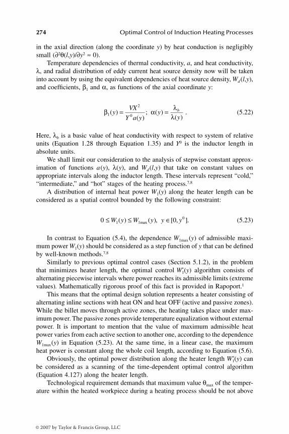
274 Optimal Control of Induction Heating Processes
in the axial direction (along the coordinate y) by heat conduction is negligiblysmall (∂2θ(l,y)/∂y2 ≈ 0).
Temperature dependencies of thermal conductivity, a, and heat conductivity,λ, and radial distribution of eddy current heat source density now will be takeninto account by using the equivalent dependencies of heat source density, Wd(l,y),and coefficients, β1 and α, as functions of the axial coordinate y:
. (5.22)
Here, λb is a basic value of heat conductivity with respect to system of relativeunits (Equation 1.28 through Equation 1.35) and Y0 is the inductor length inabsolute units.
We shall limit our consideration to the analysis of stepwise constant approx-imation of functions a(y), λ(y), and Wd(l,y) that take on constant values onappropriate intervals along the inductor length. These intervals represent “cold,”“intermediate,” and “hot” stages of the heating process.7,8
A distribution of internal heat power W1(y) along the heater length can beconsidered as a spatial control bounded by the following constraint:
(5.23)
In contrast to Equation (5.4), the dependence W1max(y) of admissible maxi-mum power W1(y) should be considered as a step function of y that can be definedby well-known methods.7,8
Similarly to previous optimal control cases (Section 5.1.2), in the problemthat minimizes heater length, the optimal control *W1(y) algorithm consists ofalternating piecewise intervals where power reaches its admissible limits (extremevalues). Mathematically rigorous proof of this fact is provided in Rapoport.1
This means that the optimal design solution represents a heater consisting ofalternating inline sections with heat ON and heat OFF (active and passive zones).While the billet moves through active zones, the heating takes place under max-imum power. The passive zones provide temperature equalization without externalpower. It is important to mention that the value of maximum admissible heatpower varies from each active section to another one, according to the dependenceW1max(y) in Equation (5.23). At the same time, in a linear case, the maximumheat power is constant along the whole coil length, according to Equation (5.6).
Obviously, the optimal power distribution along the heater length *W1(y) canbe considered as a scanning of the time-dependent optimal control algorithm(Equation 4.127) along the heater length.
Technological requirement demands that maximum value θmax of the temper-ature within the heated workpiece during a heating process should be not above
β α λλ1
2
0( )
( ); ( )
( )y
VX
Y a yy
yb= =
0 01 10≤ ≤ ∈W y W y y y( ) ( ), [ , ].max
DK6039_C005.fm Page 274 Thursday, June 8, 2006 2:31 PM
© 2007 by Taylor & Francis Group, LLC

Control of Progressive and Continuous Induction Heating Processes 275
a certain admissible value θadm. In this case, one can obtain the following expres-sion for optimal control algorithm *W1(y) that is similar to Equation (4.127):
(5.24)
Here,
, , and represent maximum admissible values of heating power density during the cold, intermediate, and hot stages of a heating process, respectively.
and are longitudinal coordinates of bound points of intermediate and hot stages.
All other denotations correspond to ones used in Expression (5.6) and Expres-sion (5.15).
Both control algorithms (Equation 5.24 and Equation 4.127) provide heatingabove Curie temperature in the typical case when holding the maximum temper-ature θmax at its maximum permissible level θadm. The following stages of a heatingcycle should be performed during the hot stage.
By analogy with Equation (5.15), one can obtain that N = 1 in Equation(5.24), if the required nonuniformity of heating ε = ε0 exceeds the difference θadm
– θ*.Assuming that the values and and yθ are given, the problem can be
reduced to determining the number, N, and lengths, , of alternatinginline sections of an induction heater. This problem can be formulated in the formof Equation (5.7) and Equation (5.8).
The shape of radial temperature distribution at the inductor exit remainsunchanged in all practicable cases when a nonlinear model (Equation 5.20 andEquation 5.21) is used. This means that the basic form of the previously describedoptimal control method could be applied for more general cases. Optimal controlresults discussed earlier for the linear IHP model (Equation 5.1 and Equation5.2) can be transferred for more complex nonlinear cases as well.
It is important to underline at this point that the temperature field variationsthat take place during the heating cycle will be described by more complicatedexpressions. Thermal equations (Equation 5.20 and Equation 5.21) should besolved after substitution of a control input function (Equation 5.24) in order to
W y
W y y
W y
1
11 1
12 1
0
*
max( )
max( )
max( )
max(
( )
, ;
,
=
< <
))max( )
max( )
max( )
;
, ;
( ),
< <
< <
y y
W y y y
W y y
2
13 2
θ
θθ << < =
+ − < <+−
y y
Wy y y jj
j j
∆10
1
13
11
21 1
;
[ ( ) ], ,max( )
==
2, .N
W11max( ) W1
2max( ) W1
3max( )
ymax( )1 ymax
( )2
ymax( )1 ymax
( )2
∆i i N, ,= 1
DK6039_C005.fm Page 275 Thursday, June 8, 2006 2:31 PM
© 2007 by Taylor & Francis Group, LLC
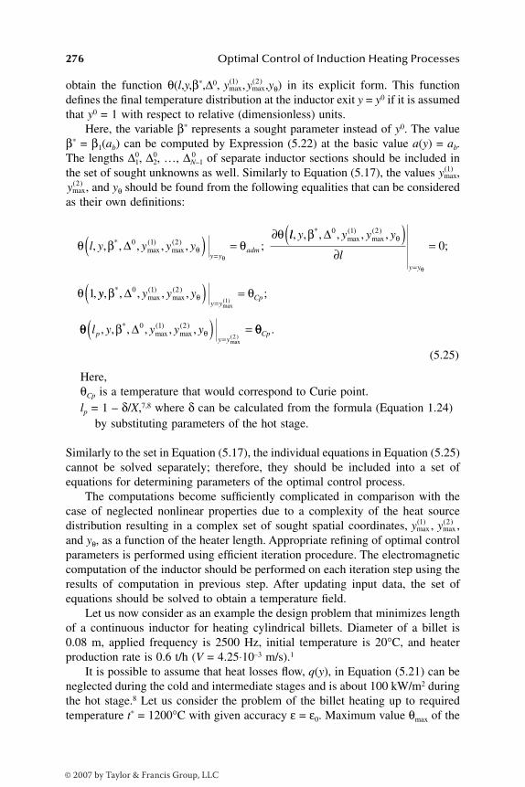
276 Optimal Control of Induction Heating Processes
obtain the function θ(l,y,β*,∆0, , ,yθ) in its explicit form. This functiondefines the final temperature distribution at the inductor exit y = y0 if it is assumedthat y0 = 1 with respect to relative (dimensionless) units.
Here, the variable β* represents a sought parameter instead of y0. The valueβ* = β1(ab) can be computed by Expression (5.22) at the basic value a(y) = ab.The lengths ∆1,
0 ∆2,0 …, ∆N–1
0 of separate inductor sections should be included inthe set of sought unknowns as well. Similarly to Equation (5.17), the values ,
, and yθ should be found from the following equalities that can be consideredas their own definitions:
(5.25)
Here,θCp is a temperature that would correspond to Curie point.lp = 1 – δ/X,7,8 where δ can be calculated from the formula (Equation 1.24)
by substituting parameters of the hot stage.
Similarly to the set in Equation (5.17), the individual equations in Equation (5.25)cannot be solved separately; therefore, they should be included into a set ofequations for determining parameters of the optimal control process.
The computations become sufficiently complicated in comparison with thecase of neglected nonlinear properties due to a complexity of the heat sourcedistribution resulting in a complex set of sought spatial coordinates, , ,and yθ, as a function of the heater length. Appropriate refining of optimal controlparameters is performed using efficient iteration procedure. The electromagneticcomputation of the inductor should be performed on each iteration step using theresults of computation in previous step. After updating input data, the set ofequations should be solved to obtain a temperature field.
Let us now consider as an example the design problem that minimizes lengthof a continuous inductor for heating cylindrical billets. Diameter of a billet is0.08 m, applied frequency is 2500 Hz, initial temperature is 20°C, and heaterproduction rate is 0.6 t/h (V = 4.25⋅10–3 m/s).1
It is possible to assume that heat losses flow, q(y), in Equation (5.21) can beneglected during the cold and intermediate stages and is about 100 kW/m2 duringthe hot stage.8 Let us consider the problem of the billet heating up to requiredtemperature t* = 1200°C with given accuracy ε = ε0. Maximum value θmax of the
ymax( )1 ymax
( )2
ymax( )1
ymax( )2
θ β θθ
θθ
l y y y yy y
adm, , , , , , ;*max( )
max( )∆0 1 2( ) =
∂
=
ll y y y y
ly y
, , , , , ,;
,
*max( )
max( )β
θ
θ
θ
∆0 1 2
0
1
( )∂
=
=
yy y y yy y
Cp, , , , , ;*max( )
max( )
max( )
β θθ∆0 1 2
1( ) ==
θθ β θl y y y ypy y
, , , , , ,*max( )
max( )
max( )
∆0 1 2
2( ) ==
θθCp .
ymax( )1 ymax
( )2
DK6039_C005.fm Page 276 Thursday, June 8, 2006 2:31 PM
© 2007 by Taylor & Francis Group, LLC
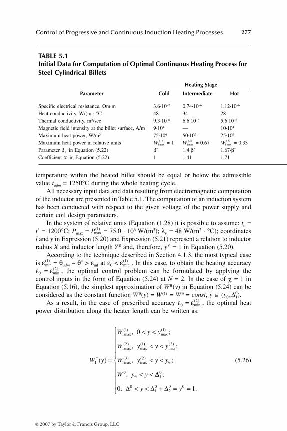
Control of Progressive and Continuous Induction Heating Processes 277
temperature within the heated billet should be equal or below the admissiblevalue tadm = 1250°C during the whole heating cycle.
All necessary input data and data resulting from electromagnetic computationof the inductor are presented in Table 5.1. The computation of an induction systemhas been conducted with respect to the given voltage of the power supply andcertain coil design parameters.
In the system of relative units (Equation (1.28) it is possible to assume: tb =t* = 1200°C; Pmax = = 75.0 ⋅ 106 W/(m3); λb = 48 W/(m2 ⋅ °C); coordinatesl and y in Expression (5.20) and Expression (5.21) represent a relation to inductorradius X and inductor length Y 0 and, therefore, y 0 = 1 in Equation (5.20).
According to the technique described in Section 4.1.3, the most typical caseis = θadm – θ* > εinf at ε0 < . In this case, to obtain the heating accuracyε0 = , the optimal control problem can be formulated by applying thecontrol inputs in the form of Equation (5.24) at N = 2. In the case of χ = 1 inEquation (5.16), the simplest approximation of W θ (y) in Equation (5.24) can beconsidered as the constant function W θ(y) = W (1) = W θ = const, y ∈ (yθ ,∆1).
0 As a result, in the case of prescribed accuracy ε0 = , the optimal heat
power distribution along the heater length can be written as:
(5.26)
TABLE 5.1Initial Data for Computation of Optimal Continuous Heating Process for Steel Cylindrical Billets
Parameter
Heating Stage
Cold Intermediate Hot
Specific electrical resistance, Om⋅mHeat conductivity, W/(m ⋅ °C.Thermal conductivity, m2/sec Magnetic field intensity at the billet surface, A/mMaximum heat power, W/m3
3.6⋅10–7
489.3⋅10–6
9⋅104
75⋅106
0.74⋅10–6
346.6⋅10–6
—50⋅106
1.12⋅10–6
285.6⋅10–6
10⋅104
25⋅106
Maximum heat power in relative unitsParameter β1 in Equation (5.22)Coefficient α in Equation (5.22)
= 1β*
1
= 0.671.4·β*
1.41
= 0.331.67·β*
1.71
W1
1
max
( ) W1
2
max
( ) W1
3
max
( )
Pmax( )1
εmin( )1 εmin
( )1
εmin( )2
εmin( )2
W y
W y y
W y
1
11 1
12 1
0
*
max( )
max( )
max( )
max(
( )
, ;
,
=
< <
))max( )
max( )
max( )
;
, ;
,
< <
< <
< <
y y
W y y y
W y y
2
13 2
θ
θθ ∆∆
∆ ∆ ∆
10
10
10
20 00 1
;
, .< < + = =
y y
DK6039_C005.fm Page 277 Thursday, June 8, 2006 2:31 PM
© 2007 by Taylor & Francis Group, LLC
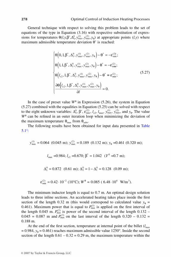
278 Optimal Control of Induction Heating Processes
General technique with respect to solving this problem leads to the set ofequations of the type in Equation (3.16) with respective substitution of expres-sions for temperatures 0θ(l,y,β*,∆1, , ,yθ) at appropriate points (l,y) wheremaximum admissible temperature deviation θ* is reached:
(5.27)
In the case of preset value W θ in Expression (5.26), the system in Equation(5.27) combined with the equalities in Equation (5.25) can be solved with respectto the eight unknown variables: 0∆1, β*, , le2, lmax, , , and yθ. The valueW θ can be refined in an outer iteration loop when minimizing the deviation ofthe maximum temperature θmax from θadm.
The following results have been obtained for input data presented in Table5.11:
(0.045 m); (0.132 m); =0.461 (0.320 m);
=0.984; =0.670; ( =0.7 m);
(0.61 m); (0.09 m);
(10°C); = 0.085 ( ).
The minimum inductor length is equal to 0.7 m. An optimal design solutionleads to three inline sections. An accelerated heating takes place inside the firstsection of the length 0.32 m (this would correspond to calculated value yθ =0.461). Maximum power that is equal to is applied on the first interval ofthe length 0.045 m. is power of the second interval of the length 0.132 –0.045 = 0.087 m and on the last interval of the length 0.320 – 0.132 =0.188 m.
At the end of the first section, temperature at internal point of the billet (lmax
= 0.984, yθ = 0.461) reaches maximum admissible value 1250°. Inside the secondsection of the length 0.61 – 0.32 = 0.29 m, the maximum temperature within the
ymax( )1 ymax
( )2
θ β θ εθ0 1 10 1 2 2, , , , , ,*
max( )
max( ) *
min(∆ y y y( ) − = − ))
*max( )
max( ) *
mi
;
, , , , , ,θ β θ εθ1 1 10 1 2∆ y y y( ) − = − nn
( )
*max( )
max( ) *
;
, , , , , ,
2
2 10 1 21θ β θθl y y ye ∆( ) − ==
∂
ε
θ β θ
min( )
*max( )
max( )
;
, , , , , ,
2
2 10 1 21l y y ye ∆(( )∂
=
l0.
εmin( )2 ymax
( )1 ymax( )2
ymax( ) .1 0 064= ymax
( ) .2 0 189= yθ
lmax le2 β* .= 1 042 Y 0
∆10 0 872= . ∆ ∆2
0101 0 128= − = .
εmin( ) .2 20 42 10= ⋅ − W θ 6 48 106. ⋅ W/m3
Pmax( )1
Pmax( )2
Pmax( )3
DK6039_C005.fm Page 278 Thursday, June 8, 2006 2:31 PM
© 2007 by Taylor & Francis Group, LLC
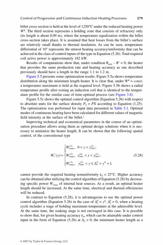
Control of Progressive and Continuous Induction Heating Processes 279
billet cross-section is held at the level of 1250°C under the reduced heating powerW θ. The third section represents a holding zone that consists of refractory only(its length is about 0.09 m), where the temperature equalization within the billetcross-section takes place. It is assumed that heat losses from the billet’s surfaceare relatively small thanks to thermal insulation. As can be seen, temperaturedifferential of 10° represents the utmost heating accuracy/uniformity that can beachieved in the class of control inputs of the type in Equation (5.26). Total requiredcoil active power is approximately 182 kW.
Results of computations show that, under condition θadm – θ* = 0, the heaterthat provides the same production rate and heating accuracy as one describedpreviously should have a length in the range 1.1 to 1.2 m.
Figure 5.5 presents some optimization results. Figure 5.5a shows temperaturedistribution along the minimum length heater. It is clear that, under W θ = const,a temperature maximum is held at the required level. Figure 5.5b shows a radialtemperature profile after exiting an induction coil that is identical to the temper-ature profile for the similar case of time-optimal process (see Figure 3.8).
Figure 5.5c shows the optimal control algorithm (Equation 5.26) with respectto absolute units for the surface density P0 = PX according to Equation (1.25).The optimization was performed for input data presented in Table 5.1. Optimalmodes of continuous heating have been calculated for different values of magneticfield intensity at the surface of the billet.1
Improving technical and economical parameters in the course of an optimi-zation procedure allows using them as optimal design solutions when it is nec-essary to minimize the heater length. It can be shown that the following spatialcontrol, of the conventional type
(5.28)
cannot provide the required heating nonuniformity ε0 < 25°C. Higher accuracycan be obtained after utilizing the control algorithm of Equation (5.28) by decreas-ing specific power W1max of internal heat sources. As a result, an optimal heaterlength should be increased. At the same time, electrical and thermal efficiencieswill be reduced.
In contrast to Equation (5.28), it is advantageous to use the optimal powercontrol algorithm (Equation 5.26) in the case of ∆1
0 = y0, ∆20 = 0, when a heating
cycle includes a stage of holding maximum temperature at the admissible level.At the same time, the soaking stage is not envisaged in this case. It is possibleto show that, for given heating accuracy ε0, which can be attainable under controlinput in the form of Equation (5.26) at ∆2 = 0, the minimum heater length as a
W y
W y y
W y1
11 1
12 1
0
*
max( )
max( )
max( )
max(( )
, ;
,=
< <
))max( )
max( )
max( )
;
, ,
< <
< ≤ = =
y y
W y y y
2
13 2
10 0 1∆
DK6039_C005.fm Page 279 Thursday, June 8, 2006 2:31 PM
© 2007 by Taylor & Francis Group, LLC

280 Optimal Control of Induction Heating Processes
FIGURE 5.5 Temperature distribution along the heater length (a); temperature distributionalong billet radius at the inductor exit (b) and optimal spatial control (c) for continuousheating of steel cylindrical billets.
0.2
(a)
0.4 0.6 0.8 1
Δ01
Δ02
Δ01
Δ02
20
300
600
900
1200
1250
t, °C
t, °C
tadm t(lmax)
t(1)
t(0)
(1) ymax (2) y
max
(1) W1 max
(1) ymax
(2) ymax
yθ
(2) W1 max
(3) W1 max
W θ
y
yθ
0 0.2 0.4
(b)
(c)
0.6 0.8 1 1200
1195
1190
1205
1210
0 0.2 0.4 0.6 0.8 1
50
100
150
200
250
300
W ⋅ 10−4, W/m2
1
0.5
y
l le2
DK6039_C005.fm Page 280 Thursday, June 8, 2006 2:31 PM
© 2007 by Taylor & Francis Group, LLC
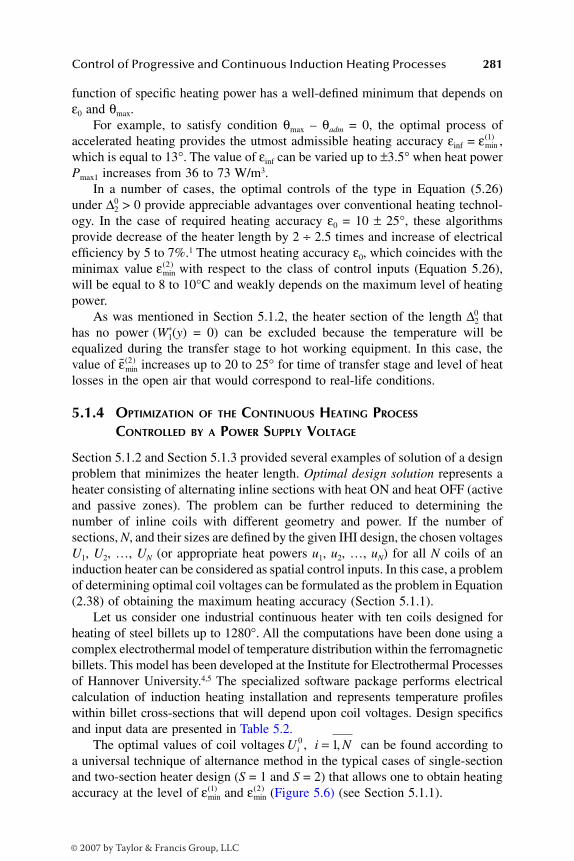
Control of Progressive and Continuous Induction Heating Processes 281
function of specific heating power has a well-defined minimum that depends onε0 and θmax.
For example, to satisfy condition θmax – θadm = 0, the optimal process ofaccelerated heating provides the utmost admissible heating accuracy εinf = ,which is equal to 13°. The value of εinf can be varied up to ±3.5° when heat powerPmax1 increases from 36 to 73 W/m3.
In a number of cases, the optimal controls of the type in Equation (5.26)under ∆2
0 > 0 provide appreciable advantages over conventional heating technol-ogy. In the case of required heating accuracy ε0 = 10 ± 25°, these algorithmsprovide decrease of the heater length by 2 ÷ 2.5 times and increase of electricalefficiency by 5 to 7%.1 The utmost heating accuracy ε0, which coincides with theminimax value with respect to the class of control inputs (Equation 5.26),will be equal to 8 to 10°C and weakly depends on the maximum level of heatingpower.
As was mentioned in Section 5.1.2, the heater section of the length ∆20 that
has no power 1(W*(y) = 0) can be excluded because the temperature will beequalized during the transfer stage to hot working equipment. In this case, thevalue of increases up to 20 to 25° for time of transfer stage and level of heatlosses in the open air that would correspond to real-life conditions.
5.1.4 OPTIMIZATION OF THE CONTINUOUS HEATING PROCESS CONTROLLED BY A POWER SUPPLY VOLTAGE
Section 5.1.2 and Section 5.1.3 provided several examples of solution of a designproblem that minimizes the heater length. Optimal design solution represents aheater consisting of alternating inline sections with heat ON and heat OFF (activeand passive zones). The problem can be further reduced to determining thenumber of inline coils with different geometry and power. If the number ofsections, N, and their sizes are defined by the given IHI design, the chosen voltagesU1, U2, …, UN (or appropriate heat powers u1, u2, …, uN) for all N coils of aninduction heater can be considered as spatial control inputs. In this case, a problemof determining optimal coil voltages can be formulated as the problem in Equation(2.38) of obtaining the maximum heating accuracy (Section 5.1.1).
Let us consider one industrial continuous heater with ten coils designed forheating of steel billets up to 1280°. All the computations have been done using acomplex electrothermal model of temperature distribution within the ferromagneticbillets. This model has been developed at the Institute for Electrothermal Processesof Hannover University.4,5 The specialized software package performs electricalcalculation of induction heating installation and represents temperature profileswithin billet cross-sections that will depend upon coil voltages. Design specificsand input data are presented in Table 5.2.
The optimal values of coil voltages can be found according toa universal technique of alternance method in the typical cases of single-sectionand two-section heater design (S = 1 and S = 2) that allows one to obtain heatingaccuracy at the level of and (Figure 5.6) (see Section 5.1.1).
εmin( )1
εmin( )2
εmin( )2
Ui0 , i N= 1,
εmin( )1 εmin
( )2
DK6039_C005.fm Page 281 Thursday, June 8, 2006 2:31 PM
© 2007 by Taylor & Francis Group, LLC
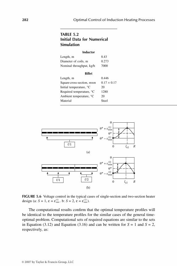
282 Optimal Control of Induction Heating Processes
The computational results confirm that the optimal temperature profiles willbe identical to the temperature profiles for the similar cases of the general time-optimal problem. Computational sets of required equations are similar to the setsin Equation (3.12) and Equation (3.16) and can be written for S = 1 and S = 2,respectively, as:
TABLE 5.2Initial Data for Numerical Simulation
InductorLength, m 8.43Diameter of coils, m 0.273Nominal throughput, kg/h 7000
BilletLength, m 0.446Square cross-section, mxm 0.17 × 0.17Initial temperature, °C 20Required temperature, °C 1280Ambient temperature, °C 20Material Steel
FIGURE 5.6 Voltage control in the typical cases of single-section and two-section heaterdesign (a: S = 1, ε = . b: S = 2, ε = ).
(a)
(1)
(1)
(2)
(2)
(b)
0 le2 R
θ∗ + εmin
θ∗ − εmin
0 le2 R
θ∗
θ
θ∗ + εmin
θ∗ − εmin
θ∗
θ
εmin( )1 εmin
( )2
DK6039_C005.fm Page 282 Thursday, June 8, 2006 2:31 PM
© 2007 by Taylor & Francis Group, LLC

Control of Progressive and Continuous Induction Heating Processes 283
(5.29)
(5.30)
These sets can be solved by conventional iteration methods with respect toall unknown variables including minimax values and . The numericalmodel allows computing the final maximum and minimum temperature deviationsfrom the required temperature θ* at nodes of the spatial mesh. All inductionheating coils should be grouped and it should be decided how many sections arenecessary and how many coils would be located in those sections.
Figure 5.7 shows how a number of inductor coils in the second controlledsection (S = 2) affects the minimax value and maximum temperature thattook place during a heating cycle.4,5 Computations have been conducted forheating of slabs with cross-section 170 mm × 170 mm at a nominal throughput
FIGURE 5.7 Minimax value and maximum temperature surplus tmax – t* as a functionof a number of coils in the second section under maximum production rate.
θ θ ε
θ θ ε
( , ) ;
( , ) ;
*min( )
*min( )
0 10 1
2 10 1
U
l Ue
− = −
− =
∂∂∂
=
θ( , );
l U
le2 1
0
0
θ θ ε
θ θ
( , , ) ;
( , , )
*min( )
*
0 10
20 2
2 10
20
U U
l U Ue
− = −
− = εε
θ θ ε
θ
min( )
*min( )
;
( , , ) ;
( ,
2
10
20 2
2 1
1 U U
l Ue
− = −
∂ 0020
0, )
.U
l∂=
εmin( )1 εmin
( )2
εmin( )2
0
100
200
300
1 2 3 4 5 6
εmin(2)
7 8 9
Number of coils in the second section
t, °C
Maximum temperature
surplus
εmin( )2
DK6039_C005.fm Page 283 Thursday, June 8, 2006 2:31 PM
© 2007 by Taylor & Francis Group, LLC
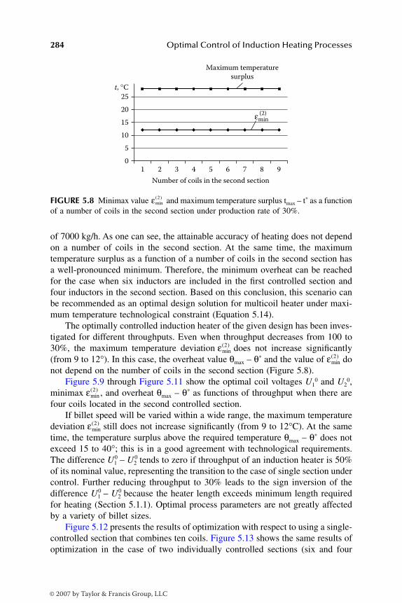
284 Optimal Control of Induction Heating Processes
of 7000 kg/h. As one can see, the attainable accuracy of heating does not dependon a number of coils in the second section. At the same time, the maximumtemperature surplus as a function of a number of coils in the second section hasa well-pronounced minimum. Therefore, the minimum overheat can be reachedfor the case when six inductors are included in the first controlled section andfour inductors in the second section. Based on this conclusion, this scenario canbe recommended as an optimal design solution for multicoil heater under maxi-mum temperature technological constraint (Equation 5.14).
The optimally controlled induction heater of the given design has been inves-tigated for different throughputs. Even when throughput decreases from 100 to30%, the maximum temperature deviation does not increase significantly(from 9 to 12°). In this case, the overheat value θmax – θ* and the value of donot depend on the number of coils in the second section (Figure 5.8).
Figure 5.9 through Figure 5.11 show the optimal coil voltages U10 and U2
0,minimax , and overheat θmax – θ* as functions of throughput when there arefour coils located in the second controlled section.
If billet speed will be varied within a wide range, the maximum temperaturedeviation still does not increase significantly (from 9 to 12°C). At the sametime, the temperature surplus above the required temperature θmax – θ* does notexceed 15 to 40°; this is in a good agreement with technological requirements.The difference U1
0 – U20 tends to zero if throughput of an induction heater is 50%
of its nominal value, representing the transition to the case of single section undercontrol. Further reducing throughput to 30% leads to the sign inversion of thedifference U1
0 – U20 because the heater length exceeds minimum length required
for heating (Section 5.1.1). Optimal process parameters are not greatly affectedby a variety of billet sizes.
Figure 5.12 presents the results of optimization with respect to using a single-controlled section that combines ten coils. Figure 5.13 shows the same results ofoptimization in the case of two individually controlled sections (six and four
FIGURE 5.8 Minimax value and maximum temperature surplus tmax – t* as a functionof a number of coils in the second section under production rate of 30%.
25
t, °C
20
15
10
5
01 2 3
Number of coils in the second section
Maximum temperature
surplus
4 5 6 7 8 9
εmin(2)
εmin( )2
εmin( )2
εmin( )2
εmin( )2
εmin( )2
DK6039_C005.fm Page 284 Thursday, June 8, 2006 2:31 PM
© 2007 by Taylor & Francis Group, LLC

Control of Progressive and Continuous Induction Heating Processes 285
coils, respectively). Figure 5.12 and Figure 5.13 show the temperature distribu-tions at optimal operating mode at the nominal throughput of 100%. Nonmonot-onous character of the surface temperature variation can be explained by inter-section gaps and nonlinear effects due to the transition between ferromagneticand paramagnetic phases of heated material at the Curie point.
When throughput decreases from nominal value to 30%, the temperaturedrops within the billet cross-section reduce significantly (Figure 5.14) becauseof sign inversion of the difference U1
0 – U20 (Figure 5.9).
FIGURE 5.9 Optimal voltages U10 and U2
0 as function of throughput in the case of fourcoils located in the second controlled section.
FIGURE 5.10 Minimax value as function of throughput in the case of four coilslocated in the second controlled section.
287
390
538 573 570
383 376 364 364 358
0
100
200
300
400
500
600
700
30 50 90 95 100
Throughput, %
Vo
ltag
e, V
12 (2)
10 9 9 9
0
2
4
6
8
10
12
30 50 90 95 100
Throughput, %
εmin
εmin( )2
DK6039_C005.fm Page 285 Thursday, June 8, 2006 2:31 PM
© 2007 by Taylor & Francis Group, LLC

286 Optimal Control of Induction Heating Processes
FIGURE 5.11 Maximum temperature surplus tmax – t* as function of throughput in thecase of four coils located in the second controlled section.
FIGURE 5.12 Temperature distribution along the heater length in the billet center (1) andat the billet surface (2) and temperature distribution along billet radius at the inductor exit(3) in the case of single-controlled section for maximum throughput at heating accuracyε = .
28
21
15
31
40
0
5
10
15
20
25
30
35
40
30 50 90 95 100
Throughput, %
tmax–t,* °C
No_1 No_2 No_3 No_4 No_5 No_6 No_7 No_8 No_9 No_10
0
140
280
420
560
700
840
980
1120
1260
t, °C
0.76 1.51 2.28 3.03 3.8 4.56 5.32 6.08 6.84 7.6
m
0
1
2 t∗3
8.4 0.17
m
εmin( )1
DK6039_C005.fm Page 286 Thursday, June 8, 2006 2:31 PM
© 2007 by Taylor & Francis Group, LLC

Control of Progressive and Continuous Induction Heating Processes 287
FIGURE 5.13 Temperature distribution along the heater length in the billet center (1) andat the billet surface (2) and temperature distribution along billet radius at the inductor exit(3) in the case of two individually-controlled sections for maximum throughput at heatingaccuracy ε = .
FIGURE 5.14 Temperature distribution along the heater length in the billet center (1) andat the billet surface (2) and temperature distribution along billet radius at the inductor exit(3) in the case of two individually-controlled sections for 30% throughput at heatingaccuracy ε = = .
No_1 No_2 No_3 No_4 No_5 No_6 No_7 No_8 No_ 9 No_ 10
0
140
280
420
560
700
840
980
1120
1260
1st section 2nd section
t, °C
0.76 1.51 2.28 3.03 3.8 4.56 5.32 6.08 6.84 7.6
m
0
1
2
t∗3
8.4 0.17
m
εmin( )2
No_1 No_2 No_3 No_4 No_5 No_6 No_7 No_8 No_9 No_10
0
140
280
420
560
700
840
980
1120
1260
1st section 2nd section
t, °C
0.76 1.51 2.28 3.03 3.8 4.56 5.32 6.08 6.84 7.6
m
0
2t∗3
8.4 0.17
m
1
εmin( )2
DK6039_C005.fm Page 287 Thursday, June 8, 2006 2:31 PM
© 2007 by Taylor & Francis Group, LLC

288 Optimal Control of Induction Heating Processes
5.2 OPTIMIZATION OF PROGRESSIVE HEATERS AT STEADY-STATE OPERATING CONDITIONS
5.2.1 KEY FEATURES OF OPTIMIZATION PROBLEMS FOR PROGRESSIVE HEATERS
Progressive multistage heating is widespread in industry. This heating modeoccurs when two or more heated workpieces (e.g., billets) are moved (via pusher,indexing mechanism, walking beam, etc.) through a single-coil or multicoil induc-tion heater. Therefore, components are sequentially heated (in a progressivemanner) at certain predetermined heating stages inside the induction heater (Sec-tion 1.3).
Within each step, the billet is heated in static position; then the billets arequickly moved to the one position further towards the coil exit. Simultaneously,one new billet is loaded into the heater and one heated billet is unloaded. Pro-gressive induction heating installations operate at the certain output cycle time.Output cycle time depends on number of billets that can be located inside theheater. The value of output cycle time can be changed during transient operatingmodes.
The heating of each billet in a progressive manner differs from static heatingby the fact that the billet is heated step by step in a number of static positionsinside a heater instead of heating in a single constant position. Therefore, atemperature distribution within the inductor load is distorted in comparison withtemperature field inside static heater due to a nonuniform distribution of heatpower along the heater length. This nonuniformity is caused by switching offpower to the heater for loading/unloading operations, air gaps between coils,electromagnetic and thermal end effects, and other phenomena unique for non-static heating mode.
It is possible to take these factors into account by using an inverted schemefor static billets heating under discrete variation of heat power in time. Thisapproach provides similarity with a movement of heated material. In this case,an optimization problem for a progressive heater at steady-state operating con-ditions can be reduced to an optimal control problem for appropriate static heatingmode. The optimal control of progressive heating can be properly considered asa time-dependent power control scanning along the heater length and representingOCP solution that takes into account peculiarities of the heater design.
The experience of computations shows1 that an inverted scheme does not leadto changes in established qualitative characteristics of optimal static heatingprocesses. This means that the type of optimal control function, basic properties,and shape of final temperature distribution remain unchanged as applied to opti-mization problems for static heating.
Based on these conclusions, the alternance method can be extended onto awide range of IHP and IHI optimization problems for progressive heaters. How-ever, essential features arise when applying the alternance method. They dealwith unique features of the progressive heating conditions.
DK6039_C005.fm Page 288 Thursday, June 8, 2006 2:31 PM
© 2007 by Taylor & Francis Group, LLC
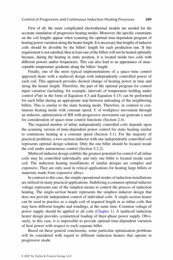
Control of Progressive and Continuous Induction Heating Processes 289
First of all, the more complicated electrothermal models are needed for theaccurate simulation of progressive heating modes. Moreover, the specific constraintson the coil lengths appear when scanning the optimal time-dependent program ofheating power variation along the heater length. It is necessary that lengths of inductorcoils should be divisible by the billets’ length for each production run. If thisrequirement is not satisfied, then at least one of the billets will not be heated optimallybecause, during the heating in static position, it is located inside two coils withdifferent powers and/or frequencies. This can also lead to an appearance of unac-ceptable temperature gradients along the billets’ length.
Finally, one of the most typical implementations of a space–time controlapproach deals with a multicoil design with independently controlled power ofeach coil. This approach provides desired change of heating power in time andalong the heater length. Therefore, the part of the optimal program for controlinput variation (including, for example, intervals of temperature holding undercontrol uθ(ϕ) in the form of Equation 4.3 and Equation 4.13) can be performedfor each billet during an appropriate step between unloading of the neighboringbillets. This is similar to the static heating mode. Therefore, in contrast to con-tinuous heating mode with constant speed, V, of workpiece movement throughan inductor, optimization of IHI with progressive movement can generate a needfor consideration of space–time control functions (Section 2.4).
The required number of inline independently controlled coils depends uponthe scanning version of time-dependent power control for static heating similarto continuous heating at a constant speed (Section 5.1). For the majority ofpractical problems, a two-section inductor with one independently controlled coilrepresents optimal design solution. Only the one billet should be located insidethe coil under autonomous control (Section 5.2.2).
Multicoil inductor design exhibits the greatest potential for control if all inlinecoils may be controlled individually and only one billet is located inside eachcoil. The induction heating installations of similar designs are complex andexpensive. They are only used in critical applications for heating large billets ormaterials made from expensive alloys.
In contrast to this case, the simple operational modes of induction installationsare utilized in many practical applications. Stabilizing a common optimal inductorvoltage represents one of the simplest means to control the process of inductionheating. The single-section heater represents the simplest inductor design thatdoes not provide independent control of individual coils. A single-section heatercan be used in practice as a single coil of required length or as inline coils thatmay have different lengths and windings, at the same time. Common voltage ofpower supply should be applied to all coils (Chapter 1). A multicoil inductionheater design provides symmetrical loading of three-phase power supply. Obvi-ously, in this case, it is impossible to provide optimal time-dependent variationof heat power with respect to each separate billet.
Based on these general conclusions, some particular optimization problemswill be considered with regard to different induction heaters that operate inprogressive mode.
DK6039_C005.fm Page 289 Thursday, June 8, 2006 2:31 PM
© 2007 by Taylor & Francis Group, LLC

290 Optimal Control of Induction Heating Processes
5.2.2 OPTIMIZATION OF INDUCTION HEATER DESIGN AND OPERATING MODES
Similarly to Chapter 3 and Chapter 4, let us consider a time-optimal controlproblem for progressive induction heating with prescribed accuracy ε at the exitof an inductor.
As was shown in Section 5.2.1, the optimal control problem for progressiveheating mode can be reduced to a time-optimal control problem for invertedscheme of static heating mode. This means that optimal control of progressiveheating can be properly considered as a time-dependent power control scanningalong the heater length. It is important to underline that all essential features andappropriate relationships between time-dependent control and spatial scanningalong the heater length should be taken into account.
The shape of the optimal control algorithm remains similar to the case ofstatic induction heating. The typical algorithm of time-optimal power control withconsideration of the “real-life” technological constraints can be represented bythe expressions in Equation (4.1) through Equation (4.5). The difference onlydeals with the expressions that describe temperature distribution. These expres-sions will be modified and become more complicated to simulate the movementof billets.
Results of computation show that, in a majority of practical cases, the firststage of time-optimal control for static heaters represents heating with maximumpower u ≡ Umax or using power close to its maximum value (in case it is necessaryto hold tensile thermal stress at admissible levels according to expressions inEquation 4.1 through Equation 4.5, Figure 4.2 through Figure 4.5, and Figure4.12). The value of ϕh represents duration of this control stage.
Let us denote the time required for heating of one billet as ϕopt0 and the
duration of one step of progressive heating (output cycle time) as ϕ*. If thefollowing condition:
, (5.31)
is satisfied, then the optimal design solution represents a heater that consists oftwo sections of different lengths.
In the first section, where B ≥ 1 billets are located simultaneously, themaximum constant voltage or voltage close to its maximum admissible value isapplied for duration Bϕ*. This stage provides intensive heating under the conditionthat the maximum value of tensile thermal stresses would not exceed prescribedadmissible value σadm.
In the second independently controlled section, only one billet of maximumlength can be located. The second control stage of duration ϕ* takes place in thissection according to the optimal control algorithm. Each section can be used inpractice as a single coil of required length or as inline coils that may have differentlengths and windings but should be fed from a common power supply. The length
ϕ ϕ ϕopt h0 − ≤ *
DK6039_C005.fm Page 290 Thursday, June 8, 2006 2:31 PM
© 2007 by Taylor & Francis Group, LLC
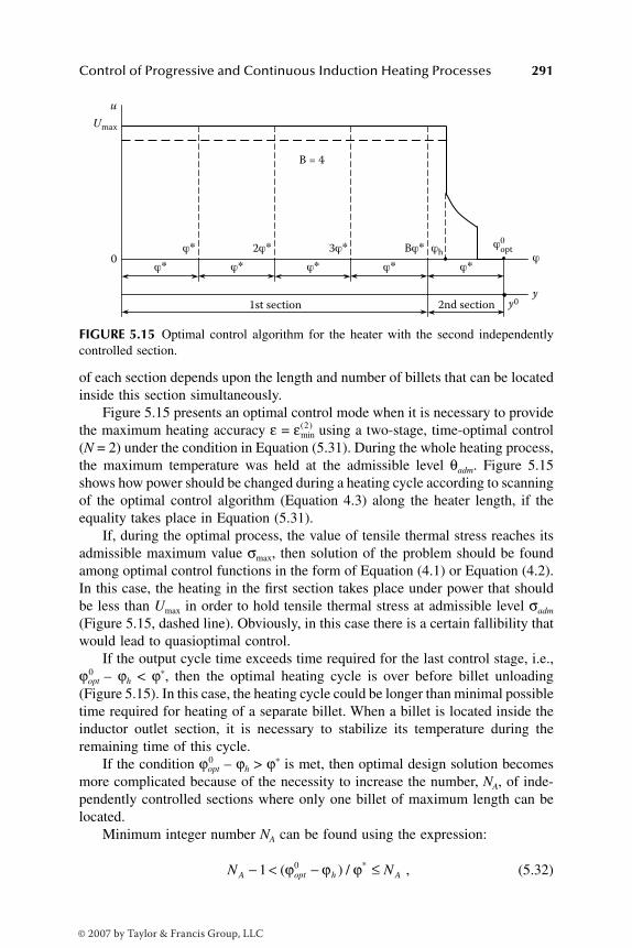
Control of Progressive and Continuous Induction Heating Processes 291
of each section depends upon the length and number of billets that can be locatedinside this section simultaneously.
Figure 5.15 presents an optimal control mode when it is necessary to providethe maximum heating accuracy ε = using a two-stage, time-optimal control(N = 2) under the condition in Equation (5.31). During the whole heating process,the maximum temperature was held at the admissible level θadm. Figure 5.15shows how power should be changed during a heating cycle according to scanningof the optimal control algorithm (Equation 4.3) along the heater length, if theequality takes place in Equation (5.31).
If, during the optimal process, the value of tensile thermal stress reaches itsadmissible maximum value σmax, then solution of the problem should be foundamong optimal control functions in the form of Equation (4.1) or Equation (4.2).In this case, the heating in the first section takes place under power that shouldbe less than Umax in order to hold tensile thermal stress at admissible level σadm
(Figure 5.15, dashed line). Obviously, in this case there is a certain fallibility thatwould lead to quasioptimal control.
If the output cycle time exceeds time required for the last control stage, i.e.,ϕopt
0 – ϕh < ϕ*, then the optimal heating cycle is over before billet unloading(Figure 5.15). In this case, the heating cycle could be longer than minimal possibletime required for heating of a separate billet. When a billet is located inside theinductor outlet section, it is necessary to stabilize its temperature during theremaining time of this cycle.
If the condition ϕopt0 – ϕh > ϕ* is met, then optimal design solution becomes
more complicated because of the necessity to increase the number, NA, of inde-pendently controlled sections where only one billet of maximum length can belocated.
Minimum integer number NA can be found using the expression:
, (5.32)
FIGURE 5.15 Optimal control algorithm for the heater with the second independentlycontrolled section.
0 ϕ∗
ϕ∗ ϕ∗ ϕ∗ ϕ∗ ϕ∗2ϕ∗ 3ϕ∗ Bϕ∗ ϕh ϕ
y y0
ϕ0opt
B = 4
2nd section 1st section
u Umax
εmin( )2
N NA opt h A− < − ≤1 0( ) / *ϕ ϕ ϕ
DK6039_C005.fm Page 291 Thursday, June 8, 2006 2:31 PM
© 2007 by Taylor & Francis Group, LLC
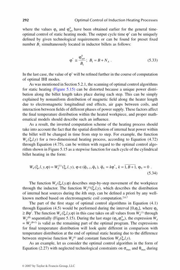
292 Optimal Control of Induction Heating Processes
where the values ϕh and ϕopt0 have been obtained earlier for the general time-
optimal control of static heating mode. The output cycle time ϕ* can be uniquelydefined by given technological requirements or can be found for preset fixednumber B1 simultaneously located in inductor billets as follows:
. (5.33)
In the last case, the value of ϕ* will be refined further in the course of computationof optimal IHI modes.
As was mentioned in Section 5.2.1, the scanning of optimal control algorithmsfor static heating (Figure 5.15) can be distorted because a unique power distri-bution along the billet length takes place during each step. This can be simplyexplained by nonuniform distribution of magnetic field along the heater lengthdue to electromagnetic longitudinal end effects, air gaps between coils, andinteraction between fields of different phases of power supply. These factors affectthe final temperature distribution within the heated workpiece, and proper math-ematical models should describe such an influence.
As a result, the inverted computation scheme of the heating process shouldtake into account the fact that the spatial distribution of internal heat power withinthe billet will be changed in time from step to step. For example, the functionWd (ξ,l,y) for a two-dimensional heating process, according to Equation (4.72)through Equation (4.75), can be written with regard to the optimal control algo-rithm shown in Figure 5.15 as a stepwise function for each cycle of the cylindricalbillet heating in the form:
.
(5.34)
The function Wd (ξ,l,y,ϕ) describes step-by-step movement of the workpiecethrough the inductor. The function Wd
(k)(ξ,l,y), which describes the distributionof internal heat sources during the kth step, can be defined a priori by any well-known method based on electromagnetic coil computation.2,6,7
The part of the first stage of optimal control algorithms in Equation (4.1)through Equation (4.5) would be performed during the interval [0,ϕh], where ϕh
≥ Bϕ*. The function Wd (ξ,l,y,ϕ) in this case takes on all values from Wd(1) through
Wd(B) sequentially (Figure 5.15). During the last stage (ϕh,ϕopt),
0 the expression Wd
= Wd(B+1) is valid as the remaining part of the optimal program. The expressions
for final temperature distribution will look quite different in comparison withtemperature distribution at the end of optimal static heating due to the differencebetween stepwise function Wd
(k) and constant function Wd(ξ,l,y).As an example, let us consider the optimal control algorithm in the form of
Equation (2.27) with neglected technological constraints on σmax and θmax during
ϕϕ* ;≅ = +opt
ABB B N
0
11
W l y W l y kd dk
k k k( , , , ) ( , , ), ( , ),( ) *ξ ϕ ξ ϕ ϕ ϕ ϕ ϕ= ∈ =−1 ,, , ,k B= + =1 1 00ϕ
DK6039_C005.fm Page 292 Thursday, June 8, 2006 2:31 PM
© 2007 by Taylor & Francis Group, LLC
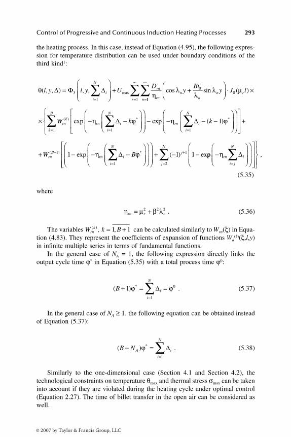
Control of Progressive and Continuous Induction Heating Processes 293
the heating process. In this case, instead of Equation (4.95), the following expres-sion for temperature distribution can be used under boundary conditions of thethird kind1:
(5.35)
where
. (5.36)
The variables can be calculated similarly to Wrn(ξ) in Equa-tion (4.83). They represent the coefficients of expansion of functions Wd
(k)(ξ,l,y)in infinite multiple series in terms of fundamental functions.
In the general case of NA = 1, the following expression directly links theoutput cycle time ϕ* in Equation (5.35) with a total process time ϕ0:
. (5.37)
In the general case of NA ≥ 1, the following equation can be obtained insteadof Equation (5.37):
. (5.38)
Similarly to the one-dimensional case (Section 4.1 and Section 4.2), thetechnological constraints on temperature θmax and thermal stress σmax can be takeninto account if they are violated during the heating cycle under optimal control(Equation 2.27). The time of billet transfer in the open air can be considered aswell.
θη
( , , ) , , maxl y l y UD
i
i
N
rn
rnn
∆ Φ ∆=
+
= =∑3
1 11
00
1
∞
=
∞
∑∑ +
⋅ ×
×
cos sin ( )λλ
λ µnn
n r
r
yBi
y J l
WW krnk
rn i
i
N
( ) *exp e− −
−=∑η ϕ∆
1
xxp ( ) *− − −
=∑η ϕrn i
i
N
k∆ 11
+
+ − − −
=
+
=
∑k
B
rnB
rn i
i
N
W B
1
1
1
1( ) *exp η ϕ∆∑∑ ∑
+ − −+
=
( ) ex1 11
2
j
j
N
pp −
=∑ηrn i
i j
N
∆
,
η µ β λrn r n= +2 2 2
W k Brnk( ), ,= +1 1
( ) *B i
i
N
+ = ==∑1 0
1
ϕ ϕ∆
( ) *B N A i
i
N
+ ==∑ϕ ∆
1
DK6039_C005.fm Page 293 Thursday, June 8, 2006 2:31 PM
© 2007 by Taylor & Francis Group, LLC

294 Optimal Control of Induction Heating Processes
The temperature distribution within the billet is distorted due to nonuniformdistribution of heat power along the heater length. This nonuniformity is causedby switching off power to the heater for loading/unloading operations, air gapsbetween coils, end effects, and other process features that are unique for nonstaticheating mode. These effects can be described if the optimal control program u*(ϕ)would be supplemented by powerless intervals where applied power u(ϕ) ≡ 0.The influence of contacts between butt-ends of billets usually can be neglected.
When nonlinear mathematical models of heating process are applied, scan-ning of time-dependent power control for static heating should be modifiedbecause the heating power depends upon temperature distribution within theworkpiece. In this case, the temperature distribution can be computed by usingthe method of successive approximations or by applying the model that describesall stages of the heating process: from the nonstationary stage under given initialconditions until the steady-state stage.1,2
As a result, the expressions for temperature distribution within each billet atthe inductor exit can be obtained in the explicit form as functions of the set ofoptimal process parameters . These functions can be calculated ana-lytically or numerically for any given inductor design. Similarly to the previouslydescribed solution, the values represent durations of stages of powercontrol functions that can be described in the form of Equation (4.1) throughEquation (4.5). These functions will be used in sets of the equation that ought tobe solved with respect to unknown process parameters . The compu-tational technique remains unchanged in comparison with that described in Chap-ter 3 and Chapter 4 with respect to static heating.
Two different statements of the time-optimal problem will arise with regardto progressive heating that describe various aspects of requirements to outputcycle time ϕ* for heated billets. Based on Expression (5.33), Expression (5.35),and Expression (5.37), one can conclude that optimal control algorithms can bedefined uniquely by using the set of parameters ∆ = (∆i), i = in the casewhen one of the values ϕ* and B1 is known a priori. Otherwise, the problem hasno single solution.
Let us assume that the number B1 of billets, which can be located simulta-neously inside the inductor of given length, is fixed. In this case, a number ofindependently controlled sections, NA, can be found by Expression (5.32) andExpression (5.33) using previously obtained results for the static heating process.A number of billets that can be located simultaneously inside the first sectionshould be calculated by the formula B = B1 – NA.
The problem can be reduced to the problem of minimizing the value *ϕmin thatprovides a minimum output cycle time under the condition that required temper-ature will be reached with desired accuracy at the inductor exit. The value ofϕmin
* can be calculated by Equation (5.38) after substitution of values ,under given numbers B and B1.
If the computations reveal that the condition in Equation (5.32) is not violatedunder obtained values ϕopt
0 and ϕh at given number NA, then the obtained designsolution should be considered as an optimal. Otherwise, the design solution should
∆i i N, ,= 1
∆i i N, ,= 1
∆i i N, ,= 1
1 N,
∆i i N0 1, ,=
DK6039_C005.fm Page 294 Thursday, June 8, 2006 2:31 PM
© 2007 by Taylor & Francis Group, LLC
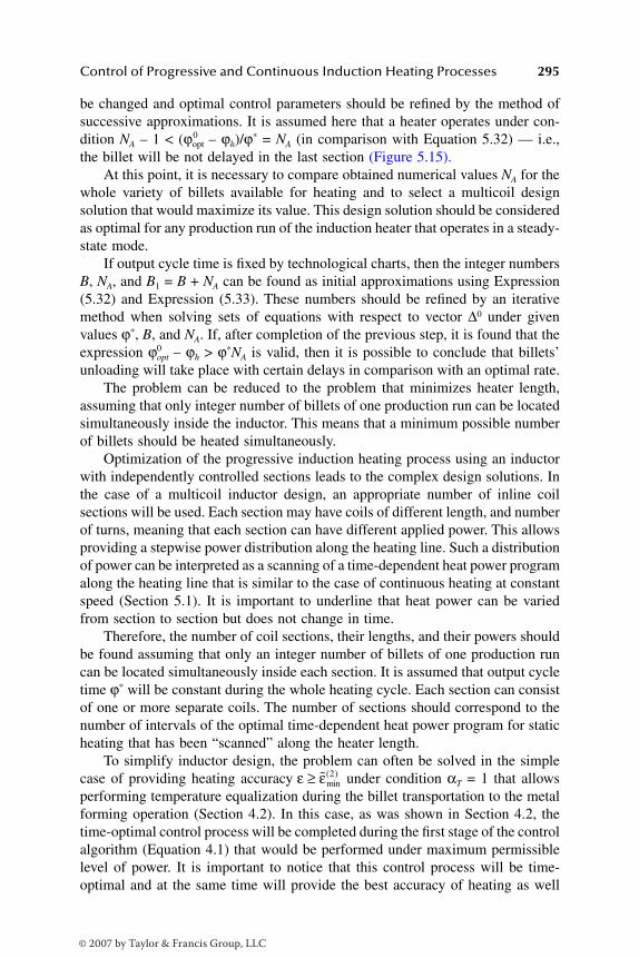
Control of Progressive and Continuous Induction Heating Processes 295
be changed and optimal control parameters should be refined by the method ofsuccessive approximations. It is assumed here that a heater operates under con-dition NA – 1 < (ϕopt
0 – ϕh)/ϕ* = NA (in comparison with Equation 5.32) — i.e.,the billet will be not delayed in the last section (Figure 5.15).
At this point, it is necessary to compare obtained numerical values NA for thewhole variety of billets available for heating and to select a multicoil designsolution that would maximize its value. This design solution should be consideredas optimal for any production run of the induction heater that operates in a steady-state mode.
If output cycle time is fixed by technological charts, then the integer numbersB, NA, and B1 = B + NA can be found as initial approximations using Expression(5.32) and Expression (5.33). These numbers should be refined by an iterativemethod when solving sets of equations with respect to vector ∆0 under givenvalues ϕ*, B, and NA. If, after completion of the previous step, it is found that theexpression ϕopt
0 – ϕh > ϕ*NA is valid, then it is possible to conclude that billets’unloading will take place with certain delays in comparison with an optimal rate.
The problem can be reduced to the problem that minimizes heater length,assuming that only integer number of billets of one production run can be locatedsimultaneously inside the inductor. This means that a minimum possible numberof billets should be heated simultaneously.
Optimization of the progressive induction heating process using an inductorwith independently controlled sections leads to the complex design solutions. Inthe case of a multicoil inductor design, an appropriate number of inline coilsections will be used. Each section may have coils of different length, and numberof turns, meaning that each section can have different applied power. This allowsproviding a stepwise power distribution along the heating line. Such a distributionof power can be interpreted as a scanning of a time-dependent heat power programalong the heating line that is similar to the case of continuous heating at constantspeed (Section 5.1). It is important to underline that heat power can be variedfrom section to section but does not change in time.
Therefore, the number of coil sections, their lengths, and their powers shouldbe found assuming that only an integer number of billets of one production runcan be located simultaneously inside each section. It is assumed that output cycletime ϕ* will be constant during the whole heating cycle. Each section can consistof one or more separate coils. The number of sections should correspond to thenumber of intervals of the optimal time-dependent heat power program for staticheating that has been “scanned” along the heater length.
To simplify inductor design, the problem can often be solved in the simplecase of providing heating accuracy under condition αT = 1 that allowsperforming temperature equalization during the billet transportation to the metalforming operation (Section 4.2). In this case, as was shown in Section 4.2, thetime-optimal control process will be completed during the first stage of the controlalgorithm (Equation 4.1) that would be performed under maximum permissiblelevel of power. It is important to notice that this control process will be time-optimal and at the same time will provide the best accuracy of heating as well
ε ε≥ min( )2
DK6039_C005.fm Page 295 Thursday, June 8, 2006 2:31 PM
© 2007 by Taylor & Francis Group, LLC

296 Optimal Control of Induction Heating Processes
as it will require the minimum of energy consumption. If we limit our consider-ation to the simplest practical algorithm (Equation 4.2), then the three-sectioninductor design (Figure 4.3) will be required.
In the first section, an accelerated heating takes place under maximum powerrestrained only by maximum permissible power level of the power supply. In thesecond and third sections, the maximum thermal stress and maximum temperaturewithin billets should be held at maximum admissible levels.
If, during the first heating stage under applying the maximum power, thetemperature maximum reaches admissible value θadm and, at the same time, thevalue σmax still remains less than σadm, then holding interval for σmax should beexcluded from the optimal control algorithm. If the first heating stage is completedbefore θmax reaches θadm, then the interval of holding of θmax should be excludedfrom the optimal heat power control algorithm.
In both cases, the two-section heater can be considered as an optimal designsolution (see algorithms in Equation 4.3 through Equation 4.5) as well as in thecase when powers of the first and second sections are slightly different. On theother hand, if the duration of interval of holding the maximum temperature isrelatively long, then there might be unacceptable accuracy of temperature stabi-lization under constant inductor power. In this case, to conduct the requiredcontrol algorithm, at least two inductor sections with different powers should beused. The final design solution can be selected by method of successive approx-imation.
Approximate values of heat powers for separate sections can be found similarto Section 5.1.2 by minimizing deviations of maximum temperature or thermalstresses from their admissible values. A simplified approach can be introducedto determine an optimal value of heat power by utilizing the conditions σmax =σadm and θmax = θadm. These conditions should be satisfied at the end of holdingintervals. Our experience shows1 that, during the whole holding stage, thisapproach guarantees that maximum temperature θmax and/or thermal stress σmax
will not exceed admissible values θadm and/or σadm. Moreover, the accuracy ofapproximation for σmax to σadm and/or θmax to θadm will also be sufficient.
If it is necessary to provide the maximum production rate for the given numberof billets located simultaneously inside the inductor, then an optimal designsolution can also be found according to the previously described technique. Aftercomputation of approximate value of ϕ* using Expression (5.33), the appropriateinitial values of number of sections and their lengths as well as numbers of billetsthat will be simultaneously located in each section can be determined.
Obtained design parameters should be in good agreement with durations ofappropriate holding intervals. Optimal design parameters can be refined by themethod of successive approximations. In each iteration step, the solutions ofappropriate sets of equations should be used in the form of Expression (5.35) forfinal temperature distribution.
Similarly to the technique described in Section 4.1, optimal values of heatpowers for separate sections can be found by using an inverted scheme for static
DK6039_C005.fm Page 296 Thursday, June 8, 2006 2:31 PM
© 2007 by Taylor & Francis Group, LLC

Control of Progressive and Continuous Induction Heating Processes 297
heating. Therefore, these values can be considered as given a priori in the courseof solving sets of equations.
In the case of fixed value ϕ*, which depends upon required heater productionrate, the time of heating inside each vth section proves to be fixed and equal to B(v)ϕ*,where is a number of billets that can be located simultaneously in thesection with number v, and r is a number of sections.
Under given values B(v), the problem can be reduced to searching for numberof sections, r, and optimal heat powers, Pv , for each separate section.
The heat power of the first section, P1, can be defined from the followingcondition that is similar to Expression (4.8):
. (5.39)
According to Equation (5.39), the maximum thermal tensile stress σmax
reaches its admissible value at the end of optimal heating stage B(1)ϕ* in the firstsection.
Expression (4.8) can be considered as an equation with respect to time ϕ1
when thermal tensile stress reaches its admissible value σmax under given maxi-mum heat power Umax. In contrast to that, Expression (5.39) can be consideredas an equation with respect to heat power P1 under given time ϕ1 = B(1)ϕ*.
Computation of the value P2 according to the suggested method can beperformed similarly to the case of P1 by using the following condition:
. (5.40)
The condition in Equation (5.40) takes place at the end of an interval whenthermal stress is held at permissible level. Unknown heat power of the secondsection can be equal to the value P2 obtained from Equation (5.40), assumingthat constraint on θmax is not violated. This would be the case if the followingcondition holds true:
. (5.41)
Otherwise, unknown value P2 can be obtained from the following expression:
. (5.42)
Resulting heat power will be less than the value of P2 that is obtained fromEquation (5.40). Therefore, the value of σmax should be reduced in comparisonwith permissible level.
B v rv( ) , ,= 1
σ ϕ σmax( ) *B adm1( ) =
σ ϕ σmax( ) ( ) *B B adm1 2+( )( ) =
θ ϕ θmax( ) ( ) *B B adm1 2+( )( ) ≤
θ ϕ θmax( ) ( ) *B B adm1 2+( )( ) =
DK6039_C005.fm Page 297 Thursday, June 8, 2006 2:31 PM
© 2007 by Taylor & Francis Group, LLC
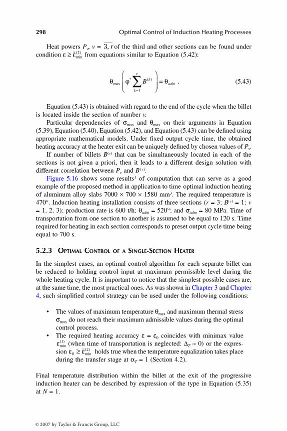
298 Optimal Control of Induction Heating Processes
Heat powers Pv, v = of the third and other sections can be found undercondition from equations similar to Equation (5.42):
. (5.43)
Equation (5.43) is obtained with regard to the end of the cycle when the billetis located inside the section of number v.
Particular dependencies of σmax and θmax on their arguments in Equation(5.39), Equation (5.40), Equation (5.42), and Equation (5.43) can be defined usingappropriate mathematical models. Under fixed output cycle time, the obtainedheating accuracy at the heater exit can be uniquely defined by chosen values of Pv.
If number of billets B(v) that can be simultaneously located in each of thesections is not given a priori, then it leads to a different design solution withdifferent correlation between Pv and B (v).
Figure 5.16 shows some results1 of computation that can serve as a goodexample of the proposed method in application to time-optimal induction heatingof aluminum alloy slabs 7000 × 700 × 1580 mm3. The required temperature is470°. Induction heating installation consists of three sections (r = 3; B(v) = 1; v= 1, 2, 3); production rate is 600 t/h; θadm = 520°; and σadm = 80 MPa. Time oftransportation from one section to another is assumed to be equal to 120 s. Timerequired for heating in each section corresponds to preset output cycle time beingequal to 700 s.
5.2.3 OPTIMAL CONTROL OF A SINGLE-SECTION HEATER
In the simplest cases, an optimal control algorithm for each separate billet canbe reduced to holding control input at maximum permissible level during thewhole heating cycle. It is important to notice that the simplest possible cases are,at the same time, the most practical ones. As was shown in Chapter 3 and Chapter4, such simplified control strategy can be used under the following conditions:
• The values of maximum temperature θmax and maximum thermal stressσmax do not reach their maximum admissible values during the optimalcontrol process.
• The required heating accuracy ε = ε0 coincides with minimax value(when time of transportation is neglected: ∆T ≈ 0) or the expres-
sion holds true when the temperature equalization takes placeduring the transfer stage at αT = 1 (Section 4.2).
Final temperature distribution within the billet at the exit of the progressiveinduction heater can be described by expression of the type in Equation (5.35)at N = 1.
3 r,ε ε≥ min
( )2
θ ϕ θmax* ( )B k
k
v
adm
=∑
=
1
εmin( )1
ε ε02≥ min
( )
DK6039_C005.fm Page 298 Thursday, June 8, 2006 2:31 PM
© 2007 by Taylor & Francis Group, LLC
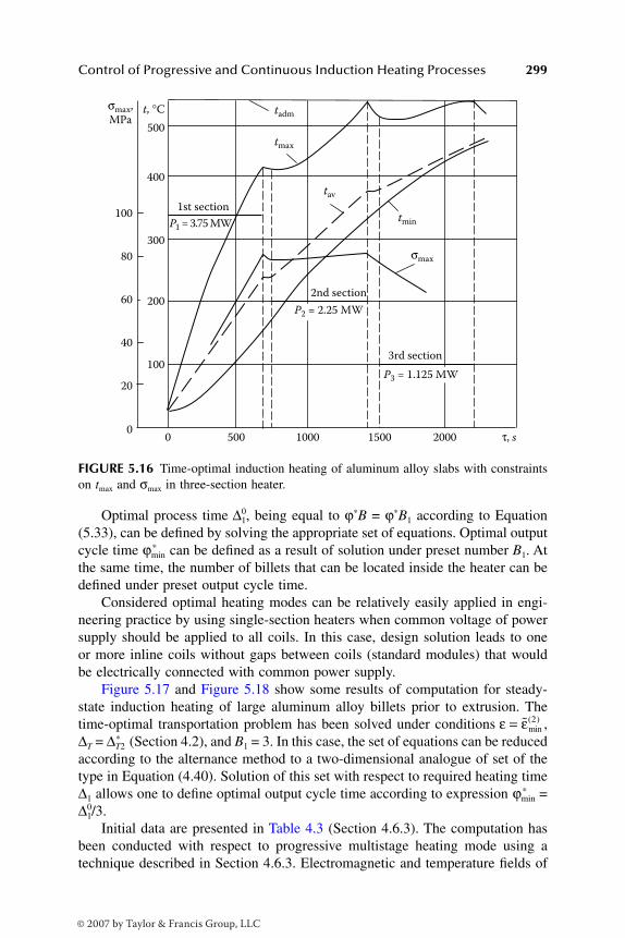
Control of Progressive and Continuous Induction Heating Processes 299
Optimal process time 0∆1, being equal to ϕ*B = ϕ*B1 according to Equation(5.33), can be defined by solving the appropriate set of equations. Optimal outputcycle time ϕmin
* can be defined as a result of solution under preset number B1. Atthe same time, the number of billets that can be located inside the heater can bedefined under preset output cycle time.
Considered optimal heating modes can be relatively easily applied in engi-neering practice by using single-section heaters when common voltage of powersupply should be applied to all coils. In this case, design solution leads to oneor more inline coils without gaps between coils (standard modules) that wouldbe electrically connected with common power supply.
Figure 5.17 and Figure 5.18 show some results of computation for steady-state induction heating of large aluminum alloy billets prior to extrusion. Thetime-optimal transportation problem has been solved under conditions ,∆T = ∆T2
* (Section 4.2), and B1 = 3. In this case, the set of equations can be reducedaccording to the alternance method to a two-dimensional analogue of set of thetype in Equation (4.40). Solution of this set with respect to required heating time∆1 allows one to define optimal output cycle time according to expression *ϕmin =∆1/3.0
Initial data are presented in Table 4.3 (Section 4.6.3). The computation hasbeen conducted with respect to progressive multistage heating mode using atechnique described in Section 4.6.3. Electromagnetic and temperature fields of
FIGURE 5.16 Time-optimal induction heating of aluminum alloy slabs with constraintson tmax and σmax in three-section heater.
00
20
40
60
80
100
σmax,
MPat, °C tadm
tmax
tmin
σmax
tav
100
200
300
400
500 1000 1500
3rd section
2nd section
1st section
P3 = 1.125 MW
P2 = 2.25 MW
P1 = 3.75 MW
2000 τ, s
500
ε ε= min( )2
DK6039_C005.fm Page 299 Thursday, June 8, 2006 2:31 PM
© 2007 by Taylor & Francis Group, LLC

300 Optimal Control of Induction Heating Processes
induction system “heater–billet” has been simulated based on a complex two-dimensional numerical model using external iteration cycle to define the outputcycle time.* The mathematical model allows taking into account switching offthe power supply for 60 s.
The induction heater consists of three inline coils without gaps between them,and common voltage of power supply is applied to all coils. Three billets can belocated simultaneously inside the inductor (Figure 5.17). Figure 5.17b shows adistribution of heat power along the heater length.
As can be seen in Figure 5.18b, the shape of final temperature distributionand number of points, where maximum temperature deviations are reached, areidentical to the temperature profile for the case of the static heating process(Section 4.5.3, Figure 4.39).
A special situation takes place in the cases of single-section heater optimi-zation, when optimal control algorithms cannot be reduced to holding voltage atconstant level. Such algorithms cannot be applied to each separate billet. Takinginto account single-section heater design, it is necessary to define the optimalcontrol algorithm that could be applied simultaneously to all billets located insidethe heater.
FIGURE 5.17 (a) Induction heating system and (b) heat power distribution along theheater length for heating of aluminum alloy billets before hot forming.
* The computations have been performed by V.B. Demidovich.
(a)
(b)
P, kW/m2
0 0.25 0.5 0.75 1.00 1.25 1.75 2.00 2.25 2.50 2.75 1.5 y, m
50
100
150
3.06
3.00
1.02 0.98 1.02
Ø0
.55
8
Ø0
.55
4
Ø0
.48
0.02 0.02
DK6039_C005.fm Page 300 Thursday, June 8, 2006 2:31 PM
© 2007 by Taylor & Francis Group, LLC
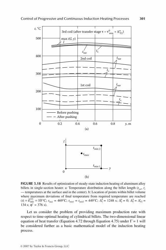
Control of Progressive and Continuous Induction Heating Processes 301
Let us consider the problem of providing maximum production rate withrespect to time-optimal heating of cylindrical billets. The two-dimensional linearequation of heat transfer (Equation 4.72 through Equation 4.75) under Γ = 1 willbe considered further as a basic mathematical model of the induction heatingprocess.
FIGURE 5.18 Results of optimization of steady-state induction heating of aluminum alloybillets in single-section heater. a: Temperature distribution along the billet length (tsur, tc
— temperatures at the surface and in the center). b: Location of points within billet volumewhere maximum deviations of final temperature from required temperature are reached( °C; tmax = 469°C; tmin1 = tmin2 = 449°C; ∆1
0 = 1248 s; ∆20 = 0; ∆T
0 = ∆T2* =
134 s; ϕ* = 376 s).
(a)
0
Before pushing
After pushing
tsur
tsur
tsur
tc
tc
tc
3rd coil (after transfer stage τ = τ0min
+ Δ∗T2
)
2nd coil
1st coil
0.2 0.4 0.6 0.8 y, m
100
200
300
400
500 max t(l, y)
t, °C
(b)
tmin 1
tmin 2
tmax
l
y0
l
ε ε= =( )min2 10
DK6039_C005.fm Page 301 Thursday, June 8, 2006 2:31 PM
© 2007 by Taylor & Francis Group, LLC

302 Optimal Control of Induction Heating Processes
Let us assume that B1 > 1 billets can be located simultaneously inside theheater. Output cycle time ϕ* would be constant during steady-state heating mode(Figure 5.19). Time required for heating of each separate billet during B1 stepsinside the inductor is equal to B1ϕ* (with neglected time of loading/unloadingoperations). Equation (4.72) through Equation (4.74) under the condition inEquation (5.34) represent temperature distribution within each billet underk = . Common control input u(ϕ), which is applied to the heater, representspower of internal heat sources or appropriate voltage of power supply. Controlu(ϕ) should be repeated on each step during steady-state mode of IHI operation.At each time point, the control u(ϕ) affects all B1 billets located inside the heater.In this case, the optimal control problem can be formulated as follows.
It is necessary to select a control function u*(ϕ) constrained by Equation (2.7)that provides steering workpiece initial temperature distribution to the desiredtemperature at the heater exit θ* with prescribed accuracy ε (according to Equation4.92) under maximum output rate (i.e., under minimum value of ϕ*). Similarlyto problems described in Chapter 4, different problem statements can be formu-lated depending upon particular situations.
Because the optimal control, u*(ϕ), should be repeated on all steps of steady-state process, heating modes for all billets are identical. Therefore, it is reasonableto consider the heating of one separate billet in order to define optimal controlalgorithms.
Obviously, during the last step before billet unloading, the optimal controlshould provide steering workpiece temperature distribution at the end of theprevious step to desired temperature (Equation 4.92) in minimal possible time.It has been proved earlier (see Section 2.8) that, within the limits of the consideredprocess step, the time-optimal control algorithm consists of alternating stages ofheating with maximum power u ≡ Umax (heat ON) and subsequent soaking/coolingunder u ≡ 0 (heat OFF) cycles. Consequently, optimal control u*(ϕ) takes theform of Equation (2.27).
Because the optimal control function u*(ϕ) is identical for all steps of thesteady-state heating process, the consequence of optimal control programs in theform of Equation (2.7) can be considered as the optimal control algorithm in thiscase. This algorithm could be improved by supplementing the process with thefurther stage of duration ∆c for performing loading/unloading operations underpower switched off.
As a result, it is possible to perform preliminary parameterization of soughtoptimal control inputs. The initial problem is reduced to searching for number,
FIGURE 5.19 Single-section progressive heater at steady-state operating conditions.
1B
loading unloading
1 B1,
DK6039_C005.fm Page 302 Thursday, June 8, 2006 2:31 PM
© 2007 by Taylor & Francis Group, LLC

Control of Progressive and Continuous Induction Heating Processes 303
N, and optimal values of parameters that uniquely specify durationsof optimal control u*(ϕ) stages.
The optimal process of heating each separate billet represents consequenceof repetitive identical stages, the number of which is equal to B1. Final temperaturedistribution can be defined by the integral expression in Equation (4.77) aftersubstitution of cyclically repeated control function u*(ϕ):
(5.44)
.
(5.45)
Here, 0∆i, i = is duration of stage with number i of N-stage control inputthat is applied during each step of steady-state heating mode.
Instead of Equation (5.35), the final temperature distribution θ(l,y,∆0) can bedescribed under the condition in Equation (5.44) and Equation (5.45) by thefollowing expression1:
(5.46)
Here, optimal output cycle time, *ϕmin, and total time, 0ϕmin, required for heatingof each billet can be obtained as the following functions of durations ∆i
0 of u*(ϕ)constancy intervals:
∆i i N0 1, ,=
u
Ujj
i
i
j
i
*
max
( )
( ) , ,
ϕ
ϕ
=
+ − < <+
=
−
∑21 1 1 0
1
1
0∆ ∆ ==
< < +
=
= =
∑
∑ ∑
1
0
1
0
1
0
1
, ;
, .
Ni
j
i
i
N
i
i
N
c∆ ∆ ∆ϕ
u v u v Bi c
i
N
* *( ), ,ϕ ϕ+ +
= =
=∑∆ ∆0
1
11 −− < < +
=∑1 0 1
0
1
, ϕ B i c
i
N
∆ ∆
1 N,
θη
l y l y UD
i
i
Nrn
rnn
, , , , max∆ Φ ∆03
0
1
( ) =
+
= =∑
111
0
0
∞
=
∞
∑∑ ( ) ×
× +
r
r
nn
n
J l
yBi
y W
µ
λλ
λcos sin rrnk
k
Bj
j
N
rn ck
( )
=
+
=∑ ∑ −( )
×
× −
1
1
1
1
1
exp *η ϕ ∆(( )( ) − −( ) +
=
−
∑exp *η ϕrn i
i
j
k 1 0
1
1
∆
×
× −
=∑exp .ηrn i
i
N
∆0
1
DK6039_C005.fm Page 303 Thursday, June 8, 2006 2:31 PM
© 2007 by Taylor & Francis Group, LLC
304 Optimal Control of Induction Heating Processes
. (5.47)
If the technological restrictions should be taken into account, then the optimalcontrol algorithm (Equation 5.44) within each process step should be complicatedand can be obtained in the form of Equation (4.1).
Problems of searching for optimal control functions uσ(ϕ) and uθ(ϕ), whichprovide holding of maximum temperature and thermal stress at their maximumpermissible levels, can be noticeably different in comparison with static heatingprocesses (Section 4.1). Under cyclically repeated control function u*(ϕ), theinitial temperature states at times ϕσ and ϕθ (when thermal stress and maximumtemperature reach their maximum permissible levels σmax and θmax) prove to bedependent on control functions uσ(ϕ) and uθ(ϕ). The following iteration procedurecan be used to solve the problem.1
Each kth approximation σuk(ϕ) and θuk(ϕ) of uσ(ϕ) and uθ(ϕ) can be foundaccording to the technique described in Section 4.1 during the step of number B1
of the heating process with respect to each separate billet. Optimal control duringall previous B1 – 1 steps is calculated for previous iterations σuk–1(ϕ) and θuk–1(ϕ).The control algorithm during B1 – 1 stages with neglected technological con-straints can be considered as the first approximation. Iterative procedure is overwhen the functions σuk(ϕ) and θuk(ϕ) coincide with σuk+1(ϕ) and θuk+1(ϕ) withrequired accuracy.
In typical cases of a transportation problem that have been considered earlier(Section 4.2) when it is necessary to provide heating accuracy at αT = 1under technological constraint on θmax, the optimal control (Equation 4.1) can bereduced to the particular form of Equation (4.3). In similar cases, during the firstheating stage under applying the maximum power, the temperature maximumreaches admissible value θadm; however, at the same time the value σmax stillremains less than σadm. Therefore, the interval of σmax holding should be excluded(Section 4.1 and Section 4.2). In contrast to Equation (4.3), the optimal controlfunction u*(ϕ) should be supplemented by the stage of duration ∆c with heatpower switched on.
The following expression can be obtained for u*(ϕ) instead of Equation (5.44)within the limits of each step:
(5.48)
Here, ϕθ and ∆10 are appropriate times within the limits of one step; the expression
in Equation (5.48) should be considered together with Equation (5.45).
ϕ ϕ ϕmin*
min min*;= + =
=∑∆ ∆i c
i
N
B0
1
01
ε ε≥ min( )2
u
U
u*
max
( )
, ;
( ), ;
,
ϕ
ϕ ϕ
ϕ ϕ ϕ
ϕ
θ
θθ=
< <
< <
< <
0
0
10
10
1
∆
∆ ∆00 +
∆c .
DK6039_C005.fm Page 304 Thursday, June 8, 2006 2:31 PM
© 2007 by Taylor & Francis Group, LLC

Control of Progressive and Continuous Induction Heating Processes 305
Figure 5.20 shows a general view of the optimal control algorithm u*(ϕ) inthe form of Equation (5.48) and Equation (5.45) with respect to heating of eachseparate billet.
If the control input function uθ(ϕ) is written in the form of Equation (4.13),then final temperature distribution at the heater exit can be represented insteadof Equation (5.46) by the following expression, which is similar to Equation(4.15) and Equation (4.16)1:
(5.49)
Using an analogy to the previously described transportation problem (Section4.2), a time, ∆T , of billet transfer to hot forming equipment can be taken intoaccount.
Our experience shows that properties of final spatial temperature distributionremain unchanged in comparison with properties established in Chapter 3and Chapter 4 in the case of static heating processes. Thus, the computational
FIGURE 5.20 Optimal control algorithm for single-section progressive heater at steady-state operating conditions.
0 ∆0
1 ∆0
1
∆C
∆01
u∗
uθ
Umax
ϕθ ϕ
θη
( , , ) , , maxl y l y UD
i
i
Nrn
rnn
∆ Φ ∆03
0
1
=
+
= =∑
11
00
1
∞
=
∞
∑∑ +
×
×
J l yBi
y
W
r nn
n
r
( ) cos sinµ λλ
λ
rrnk
rn c
k
B
k( ) exp ( )( ) exη ϕθ + − +( )( ) −
=∑ 1 1
0
1
1
∆ ∆ pp ( )( )
exp ( (
η
ηθ
rn c
rn
k
a k k
− +( ) +
+ +
1 10
10
∆ ∆
∆ −−( ) − + − +( )( )( ) +1 1 10) ) exp ( )( )∆ ∆ ∆c rn c
rkbη ϕ η
θθ nn
rn
rn ck k
η β
β η
θ
θ
−×
× − + + −( ) −exp ( )( ( ) ) exp (∆ ∆10 1 −− + + − +( )( ) ×
× +
β η ϕ
β ϕ
θ θ
θ θ
rn ck)( ( )( ))
exp ( (
1 10∆ ∆
kk c rn i
i
N
− +( ) −
=∑1 1
0 0
1
)( )) exp∆ ∆ ∆η
.
DK6039_C005.fm Page 305 Thursday, June 8, 2006 2:31 PM
© 2007 by Taylor & Francis Group, LLC
306 Optimal Control of Induction Heating Processes
technique remains unchanged in comparison with that described in Chapter 3 andChapter 4 with respect to static heating. High generality of the results obtainedin Section 3.7 allows one to extend an area of application of the alternance methodonto the considered problem.
5.2.4 TWO-POSITION CONTROL OF SLAB INDUCTION HEATING
Optimization of a progressive induction heating process using an inductor withindependently controlled inline sections of different powers has been providedin Section 5.2.2. As was mentioned in Section 5.2.1, multicoil inductor designexhibits the greatest potential for control if all inline coils may be controlledindividually and only one billet is located inside each coil. Within each step, thebillet is heated in static position inside one coil, and then billets are quicklymoved to the next coil further towards the inductor exit. The required heatingmode can be provided by applying autonomous voltage control to each coilseparately. The difference with optimal static heating only deals with effects ofbreaks needed for billets’ movement from one coil to another.
If gaps between coils are large enough, then loading/unloading operationscan be performed separately, thus allowing one to use workpiece positioninginside the coil as an additional means of spatial control of induction heating.
Two-position slab heating can serve as a good example of effective use ofthis type of spatial control.9 According to this approach, a slab is heated insidetwo separate coils, and the angle between slab axis inside the second coil andvector of magnetic intensity is equal to 90°. The temperature profiles along theslab length and width are affected by, among other factors, a distortion of elec-tromagnetic field at its end and edge areas. These effects and the field distortioncaused by them are primarily responsible for nonuniform temperature profileswithin the slab. In the case of two-position heating, the temperature gradientsdue to end and edge effects can be compensated (Figure 5.21a). As a result, theheating accuracy becomes higher than in continuous two-section heater underconstant in time maximum voltages applied to both coils.
Figure 5.21b shows some results of computation in application to two-posi-tion heating of A6 alloy slabs 1250 × 1250 × 200 mm3; frequency is 50Hz andactive power of each coil is 200 kW.1
A special piecewise linear three-dimensional model that takes into accountsurface heat-generating sources has been used to describe temperature distributionwithin the slab. As can be seen, heating nonuniformity reduces at the slab’s surfacedue to reorientation of slab in space, which means the use of the longitudinalend effect as a means of control.
Durations of stages of applied voltage constancy can be considered in thiscase as control parameters as well as one additional parameter, Kp. This parametercharacterizes optimal heating mode and shows how the longitudinal end effectacts.1,9 Factor Kp can be considered as a relation of average values of surface heatpower densities in central part and longitudinal end effect area of heated slab,and can be calculated according to limiting values of these densities PA and PB
DK6039_C005.fm Page 306 Thursday, June 8, 2006 2:31 PM
© 2007 by Taylor & Francis Group, LLC

Control of Progressive and Continuous Induction Heating Processes 307
(Figures 5.21a). The value of Kp can be changed by different means of spatialcontrol, including but not limited to different electrical connections, coil over-hang, etc.
In the simplest case of single-stage voltage control, it is necessary to provideheating accuracy ε = under the condition that time, ∆′, required for heatinginside the first coil is equal to appropriate time, ∆″, that is required for heatinginside the second coil. Values of Kp are the same for both cases of slab positioning
FIGURE 5.21 Two-position heating of slabs. a: Heat power distribution at slab surfacefor longitudinal and transversal orientation of vector of magnetic intensity. b: Time–tem-perature history for different points.
(a)
(b)
PA
z z
x x
dd d
d
y y
PA
PAPB
PB
PA
PB
PB
HI
HII
t, °C
0
100
200
300
400
10025 50 75 τ, s
2
3 4
HII
HI
1
∆′
∆″
∆T
∆T234
1
εmin( )1
DK6039_C005.fm Page 307 Thursday, June 8, 2006 2:31 PM
© 2007 by Taylor & Francis Group, LLC

308 Optimal Control of Induction Heating Processes
inside the coils. Computations of the time-optimal process of slab heating canbe performed according to the general scheme of alternance method.
The set of equations written for final temperatures should be solved withrespect to three unknown variables: ∆ = ∆′ = ∆″, Kp and . It is important tonote that optimal value of ∆ defines optimal output cycle time of the heatingsystem.
The problem becomes more complicated in comparison with previously con-sidered problems due to necessity to apply models of temperature fields asfunctions of ∆ and Kp. At the same time, the shape of final spatial temperaturedistribution within the slab cannot be found easily.
In contrast to problems considered in Section 4.5.4, for final temperaturedistribution under ε = , there will be (according to the basic condition inEquation 3.40) three points within slab volume where maximum admissibledeviations of final temperature from the required one are reached. In this case,two sought parameters, ∆ and Kp, should be found. In a typical case, only twopoints with maximum temperature deviations exist under control by commoninductor voltage, and only a single unknown parameter ∆ should be found.
REFERENCES
1. Rapoport, E.Ya., Optimization of Induction Heating of Metal, Metallurgy, Mos-cow, 1993.
2. Nemkov, V.S. and Demidovich, V.B., Theory and Computation of Induction HeatingInstallations, Energoatomizdat, St. Petersburg, 1988.
3. Rapoport, E.Ya., Alternance properties of optimal temperature distribution andcomputational algorithms in problems of induction heating processes parametricoptimization, Proc. Int. Induction Heating Semin. (IHS-98), Padua, 443, 1998.
4. Pleshivtseva, Yu.E. et al., Potentials of optimal control techniques in inductionthrough heating for forging, Proc. Int. Sci. Colloquium Modeling Electromagn.Process., Hannover, 145, 2003.
5. Pleshivtseva, Yu.E. et al., Optimal control techniques in induction through heatingfor forging, in Proc. Int. Symp. Heating Electromagn. Sources HES-04, Padua,97, 2004.
6. Rudnev, V.I. et al., Handbook of Induction Heating, Marcel Dekker, New York,2003.
7. Sluhotskii, A.E., Nemkov, V.S., Pavlov, N.A., and Bamunauer, A.V., InductionHeating Installations, Energoatomizdat, St. Petersburg, 1981.
8. Pavlov, N.A., Engineering Thermal Computation of Induction Heaters, Energia,Moscow, 1978.
9. Nemkov, V.S. et al. End effects as a means for control of induction heatingprocesses of rectangular shape workpieces, in Algoritmy i systemi upravlenijatehnologicheskimi processami v mashinostroenii, Kujbyshev, 141, 1986.
εmin( )1
εmin( )1
DK6039_C005.fm Page 308 Thursday, June 8, 2006 2:31 PM
© 2007 by Taylor & Francis Group, LLC

309
6
Combined Optimization of Production Complex for Induction Billet Heating and Subsequent Metal Hot Forming Operations
This section discusses a system approach for optimization of induction heaters.This system approach takes into consideration the whole sequence of the inter-related technological operations including billet heating by induction, its coolingduring transportation, and subsequent plastic deformation during hot working.All these subsequent processes will be considered as a technological complexand combined optimization criteria will be used for its optimization. Dependingupon application, metal hot working operations may be represented by forging,rolling, stamping, upsetting, extrusion, and other operations where metal under-goes plastic deformation.
For a particular technological complex, it is important to reveal the costfunction for each operation or stage of the technological process. As was men-tioned in Section 2.2, a proper selection of local cost function for IHI optimizationis based upon valid decomposition of a combined optimization problem
intoseparate optimization problems for processes of heating and hot working.
A local problem of IHI optimization could be solved only within the rigidframe of a priori given technological instructions. This means that optimal controlinputs can be found only in the case when required final temperature distributionof heated billets is a priori known
.
Initial temperature distribution at the beginning of the billet transportationstage complies with final temperature distribution at the end of the heating stage.The temperature distribution before the hot forming complies with final temper-ature distribution at the end of the billet transportation stage. These facts areimperative to bind workpiece temperature states during all stages of the “inductionheating–metal hot forming” technological cycle.
As most metal forming processes, hot working operations impose certainrequirements for initial temperature distribution. For example, there is the max-
DK6039_C006.fm Page 309 Thursday, June 8, 2006 3:14 PM
© 2007 by Taylor & Francis Group, LLC
310
Optimal Control of Induction Heating Processes
imum range of admissible temperature variations within the heated workpieceprior to its hot forming. The temperature distribution within a heated billet beforethe forming stage affects essentially the overall performance index of a techno-logical complex. Required temperature distribution at the inductor exit is con-strained by preset technological requirements. As a result, the value of overallcost function can deviate from the optimum one.
New possibilities appear when solving a general optimization problem withrespect to combined technical and economic indexes of complex operation as awhole. A technical index can be represented by such criteria as maximum pro-duction, minimum required floor space, utilization of existing power supplysources, minimum power consumption, and others. An economical index can berepresented by cost criteria, metal loss minimization criteria, etc.
A general optimization problem can be solved under condition of having amaximum freedom in choosing parameters of heating and hot forming operations.In this case, it might be possible to find optimal parameters (according to certainoptimization criteria) of each operation as standalone process as well.
If a designer has unlimited freedom in choosing the final thermal conditionof a heated billet, then it is possible to:
• Reveal local cost functions for optimization of IHI and deformingequipment separately, utilizing means of valid system decomposition
• Find the final temperature distribution within a heated billet that isoptimal with respect to overall cost function
• Define control inputs during the stages of heating and hot forming thatprovide desired temperature distribution and hold overall cost functionat extremum value
The described approach requires determining capabilities of a control algo-rithm out of the framework of traditional “servicing” of technology and ensuresactive participation in technology formation. This system approach deals withfinding optimal technological parameters within process flow sheets and optimaldesign of a technological site to provide optimal operational modes for eachseparately considered technological operation.
1–6
Optimization of a technological complex of induction heating of cylindrical
billets and subsequent hot forming operation using hydraulic presses will be usedas an example of application of alternance method.
5,6
6.1 MATHEMATICAL MODELS OF CONTROLLED PROCESSES
The ultimate goal of optimal control strategy is to provide required thermalconditions of workpieces just before hot working operations.
7
This is the reasonwhy the temperature distribution within the billet can be regarded as an output-controlled function. Therefore, as a subject of optimal control, a technological
DK6039_C006.fm Page 310 Thursday, June 8, 2006 3:14 PM
© 2007 by Taylor & Francis Group, LLC
Combined Optimization of Production Complex
311
complex “induction heater–hot forming” can be described by a system of heattransfer equations that represent heating, cooling (billet transfer), and hot formingstages (see Figure 2.5).
Required accuracy of temperature distribution within the billet is usuallyprovided by an acceptable level of three-dimensional temperature variations. Forthe majority of practical applications, the temperature distribution within theheated workpiece can be described by two- and three-dimensional mathematicalmodels. The majority of induction billet heaters utilize multiturn solenoid-typeinduction coils. Because they are electromagnetically long systems, such induc-tors typically have unappreciative temperature variations along the billet perim-eter due to symmetrical positioning of billets inside inductors. Therefore, a two-dimensional mathematical model can be effectively applied for mathematicalmodeling of cylindrical systems. Two-dimensional models provide sufficientinformation regarding temperature profiles in axial and radial directions.
Temperature of cylindrical billet
θ
1
(
l
,
y
,
ϕ
) during a heating process can bedescribed by the following system of two-dimensional heat transfer equations(Equation 4.72 through Equation 4.75) for
Γ
= 1 (Figure 4.37):
(6.1)
(6.2)
(6.3)
Here,
ϕ
10
is required total heating time; Biot number
Bi
h
corresponds to heat lossesfrom the surface of the billet during the whole heating process inside the inductionheater.
Temperature distribution during billet transportation stage
θ
2
(
l
,
y
,
ϕ
) can alsobe described by Equation (6.1) except that there are no heat sources:
∂∂
= ∂∂
+ ∂∂
+θ ϕϕ
θ ϕ θ ϕ12
12
11( , , ) ( , , ) ( , , )l y l y
l l
l y
l
++ ∂∂
+
∈
β θ ϕ ξ ϕ22
12
0 1
( , , )( , , ) ( );
, ( , );
l y
yW l y u
l y
d
00 10< ≤ϕ ϕ ;
∂∂
= −( ) ∂∂
θ ϕ θ θ ϕ θ ϕ11
111
0( , , )( , , ) ;
( , , )y
lBi y
y
lh a ==
∂∂
= −( )
− ∂
0
11
0
11
1
;
( , , )( , , ) ;
( ,
θ ϕ θ θ ϕ
θ
l
yBi l
l
h a
,, )( , , ) ;
ϕ θ θ ϕ∂
= −( )
y
Bi lh a 1 0
θ θ1 100( , , ) ( , ).l y l y=
DK6039_C006.fm Page 311 Thursday, June 8, 2006 3:14 PM
© 2007 by Taylor & Francis Group, LLC

312
Optimal Control of Induction Heating Processes
(6.4)
(6.5)
(6.6)
Time
∆
T
should be considered here as a total transportation time. Heat losses duringthe billet transfer stage can be estimated by value
Bi
T
that vastly increases incomparison with heat losses inside the induction coil (
Bi
T
>
Bi
h
). The thermalrefractory located inside the induction coil noticeably reduces surface heat losses.In contrast, there will be intensive surface cooling during billet transportation on air.
Both heat transfer equations (Equation 6.1 and Equation 6.4) are comple-mented by boundary conditions of the third kind (Equation 6.2 and Equation 6.5).Appropriate value of Biot criterion
Bi
T
>
Bi
h
takes into consideration an increaseof heat losses from the billet surface during billet transportation from heatingoperation to metal hot forming stage.
To simplify the study, the ambient temperature in Equation (6.2) and Equation(6.5) is considered as uniform within billet surface and equal to constant value
θ
a
.The linear axis-symmetric model of temperature distribution
θ
3
(
l
,
y
,
ϕ
) withinthe cylindrical billet during the process of pressing can be described by thefollowing two-dimensional heat transfer equation
6,8
:
(6.7)
with boundary and initial conditions similar to Equation (6.2), Equation (6.3),Equation (6.5), and Equation (6.6):
∂∂
= ∂∂
+ ∂∂
+θ ϕϕ
θ ϕ θ ϕ22
22
21( , , ) ( , , ) ( , , )l y l y
l l
l y
lββ θ ϕ
ϕ ϕ ϕ
22
22
10
100 1
∂∂
∈ ≤ ≤ +
( , , );
, ( , ); ;
l y
y
l y T∆
∂∂
= −( ) ∂∂
θ ϕ θ θ ϕ θ ϕ22
211
0( , , )( , , ) ;
( , , )y
lBi y
y
lT a ==
∂∂
= −( )
− ∂
0
11
0
22
2
;
( , , )( , , ) ;
( ,
θ ϕ θ θ ϕ
θ
l
yBi l
l
T a
,, )( , , ) ;
ϕ θ θ ϕ∂
= −( )
y
Bi lT a 2 0
θ ϕ θ ϕ2 10
1 10( , , ) ( , , ).l y l y=
∂∂
= ∂∂
+ ∂∂
+θ ϕϕ
θ ϕ θ ϕ32
32
31( , , ) ( , , ) ( , , )l y l y
l l
l y
lββ θ ϕ
γ β θ ϕ
22
32
3
∂∂
−
− ∂∂
( , , )
( , , )( , , )*
l y
y
V l y Vl y
y P yyV l y V
l y
lW l y V
l y
l P P− ∂∂
+
∈
γ θ ϕ* *( , , )( , , )
( , , );
,
3
(( , );0 1 10
20ϕ ϕ ϕ+ ≤ ≤∆T
DK6039_C006.fm Page 312 Thursday, June 8, 2006 3:14 PM
© 2007 by Taylor & Francis Group, LLC

Combined Optimization of Production Complex
313
(6.8)
(6.9)
Here, in contrast to Equation (6.1), instead of internally generated heating power
W
d
(
ξ
,
l
,
y
)
u
(
ϕ
), a volume density of heat sources
W
*
(
l
,
y
,
V
P
) is used in Equation(6.7). The density of heat sources
W
*
(
l
,
y
,
V
P
) is defined by energy of plasticdeformation of metal during the direct extrusion with speed
V
P
.The value of
W
*
(
l
,
y
,
V
P
) can be calculated by expression
8–10
:
, (6.10)
where
L
is intensity of the tangential stresses under plastic deformation and
H
isintensity of velocity of shear deformation during pressing.
The differential operator in the right side of Equation (6.1) is complementedin Equation (6.7) by components that take into account velocities
V
l
and
V
y
ofthe metal flow in radial and axial directions, respectively. Field of velocities isnonuniformly distributed within the billet volume during the pressing process.
Heat losses can be estimated by values
Bi
,
Bi
1
, and
Bi
0
of Biot criterion inboundary conditions in Equation (6.7). The ambient temperatures
0
θ
a
,
0
θ
a
1
,
0
θ
a
0
atlateral surface (
l
= 1,
y
∈
[0,1]) and at butt-ends (
y
= 1,
l
∈
[0,1]) and
y
= 0,
l
∈
[0,1]) represent appropriate calculated values (Figure 4.37).The density of heat flow
q
(
y
,
V
p
) caused by contact friction is taken intoaccount in the boundary condition in Equation (6.8).
8–10
Values
V
p
,
V
l
,
V
y
, and
W
*
in Equation (6.7) should be calculated as fractions of appropriate basic values
V
δ
and
W
δ
*
, where
W
δ
*
replaces
P
max
in formulas in Equation (1.28), Equation(1.29), Equation (1.33), and Equation (1.35). The factor
β
can be found from thecorrelation in Equation (4.76), and
γ
*
is defined by the equality
,
where
a
is the factor of temperature conductivity.The final product of technological complex “induction heater–hot working
equipment” is a press product with length
z
that can be defined according to:
∂∂
= −( ) + ∂θ ϕ θ θ ϕ θ3 03
311
( , , )( , , ) ( , );
(y
lBi y q y Va P
000
113
1 10
3
, , );
( , , )( , , )
y
l
l
yBi la
ϕ
θ ϕ θ θ ϕ
∂=
∂∂
= −( ))
− ∂∂
= −( )
;
( , , )( , , ) ;
θ ϕ θ θ ϕ30 0
03
00
l
yBi la
θ ϕ θ ϕ3 10
2 10( , , ) ( , , ).l y l yT T+ = +∆ ∆
W l y V LH l y VP P* ( , , ) ( , , )=
γ δ* = XV
a
DK6039_C006.fm Page 313 Thursday, June 8, 2006 3:14 PM
© 2007 by Taylor & Francis Group, LLC

314 Optimal Control of Induction Heating Processes
. (6.11)
Here, k is elongation ratio7 and the required value of z(ϕ2)0 is equal to zend at the
end of pressing stage ϕ = 0ϕ2.Metal heating processes impose two general requirements with regard to the
temperature distribution during heating processes. The first requirement of thetype in Equation (2.11) demands that the maximum value of the temperaturewithin a heated workpiece should be not above a certain admissible value θadm.According to the second restraint in the form of Equation (2.13), the temperaturedifferences within the whole volume of a heated workpiece should be restrictedduring heating in such a way that the maximum value of tensile thermal stresseswould not exceed prescribed admissible value σadm (see Section 2.5.2). Therestraints in Equation (2.11) and Equation (2.13) can be rewritten as follows:
(6.12)
Temperature within the heated workpiece during extrusion is restricted bymaximum admissible temperature in the die hole θcr:
. (6.13)
This requirement demands that the maximum temperature θ3(lk,1,ϕ) in thedie deformation zone (l = lk, y = 1, 0 < lk < 1) (see Figure 6.2) should not exceedadmissible limit θ3cr . Violation of these conditions could result in typical irre-versible spoilage of product, i.e., crack development.10
Due to certain technical limitations that deal with power of press, instrumentstrength, temperature interval of metal plasticity, and other factors, it is possibleto perform extrusion only in the case when initial temperature states belong to acertain region Ω:
θ3(l, y, ϕ10 + ∆T) ∈ Ω . (6.14)
Heating power u(ϕ) and ram speed Vp(ϕ) can be considered as control inputsfor heating and extrusion processes. The values of these control inputs are alsorestricted by certain admissible values Umax and Vpmax:
(6.15)
dz
dkV z z zp T endϕ
ϕ ϕ= + = =; ( ) ; ( )10
200∆
max ( , , ) ; max ( ,, [ , ] , [ , ]l y
adml y
l y l∈ ∈
≤0 1
10 1
θ ϕ θ σ yy adm, ) ; .ϕ σ ϕ ϕ≤ ≤ ≤0 10
θ ϕ θ ϕ ϕ ϕ3 3 10
201( , , ) ,lk cr T≤ + ≤ ≤∆
0 0
0
10
10
≤ ≤ ≤ ≤
≤ ≤ + ≤ ≤
u U
V Vp p T
( ) , ;
( ) ,
max
max
ϕ ϕ ϕ
ϕ ϕ ϕ∆ ϕϕ20 .
DK6039_C006.fm Page 314 Thursday, June 8, 2006 3:14 PM
© 2007 by Taylor & Francis Group, LLC
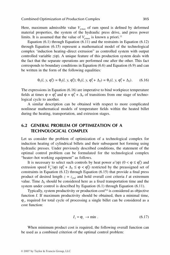
Combined Optimization of Production Complex 315
Here, maximum admissible value Vpmax of ram speed is defined by deformedmaterial properties, the system of the hydraulic press drive, and press powerlimits. It is assumed that the value of Vpmax is known a priori.11
Equation (6.1) through Equation (6.11) and the restraints in Equation (6.12)through Equation (6.15) represent a mathematical model of the technologicalcomplex ‘induction heating–direct extrusion” as controlled system with outputcontrolled variable z(ϕ). A unique feature of this production system deals withthe fact that the separate operations are performed one after the other. This factcorresponds to boundary conditions in Equation (6.6) and Equation (6.9) and canbe written in the form of the following equalities:
θ1(l, y, 0ϕ1) = θ2(l, y, 0ϕ1); θ3(l, y, 0ϕ1 + ∆T) = θ2(l, y, 0ϕ1 + ∆T). (6.16)
The expressions in Equation (6.16) are imperative to bind workpiece temperaturefields at times ϕ = ϕ1
0 and ϕ = ϕ10 + ∆T of transitions from one stage of techno-
logical cycle to another.A similar description can be obtained with respect to more complicated
nonlinear mathematical models of temperature fields within the heated billetduring the heating, transportation, and extrusion stages.
6.2 GENERAL PROBLEM OF OPTIMIZATION OF A TECHNOLOGICAL COMPLEX
Let us consider the problem of optimization of a technological complex forinduction heating of cylindrical billets and their subsequent hot forming usinghydraulic presses. Under previously described conditions, the statement of theoptimal control problem can be formulated for the technological complex“heater–hot working equipment” as follows.
It is necessary to select such controls by heat power u*(ϕ) (0 < ϕ ≤ 0ϕ1) andextrusion speed Vp
*(ϕ) (ϕ10 + ∆T ≤ ϕ < 0ϕ2) restricted by the preassigned set of
constraints in Equation (6.12) through Equation (6.15) that provide a final pressproduct of desired length z = zend and hold overall cost criteria I at extremumvalue. Time ∆T should be considered here as a fixed transportation time and thesystem under control is described by Equation (6.1) through Equation (6.11).
Typically, system productivity or production cost5,6 is considered as objectivefunction I. If maximum productivity should be obtained, then a minimal time,ϕc, required for total cycle of processing a single billet can be considered as acost function:
. (6.17)
When minimum product cost is required, the following overall function canbe used as a combined criterion of the optimal control problem:
I c1 = →ϕ min
DK6039_C006.fm Page 315 Thursday, June 8, 2006 3:14 PM
© 2007 by Taylor & Francis Group, LLC

316 Optimal Control of Induction Heating Processes
. (6.18)
This criterion (Equation 6.18) includes all cost components withweighting coefficients Ci. Those coefficients make sense with respect to a relativecosting (that is a function of control inputs) representing an importance of eachof the overall costs. Increase of the heating time leads to expense growth, accord-ing to the criterion (Equation 6.17) with correspondent weight coefficients Ct.The value of Pi is primarily defined by energy expenses for heating and pressing,as well as by metal losses due to scale formation during the process of heating(see Section 2.9.2, Section 3.5, and Section 4.4.1).
The formulated problem provides freedom in choosing the billet temperatureθ2(l,y,ϕ1
0 + ∆T) before the hot forming stage in a way that would satisfy require-ments imposed by heating and hot working operations (with regard to transpor-tation time). An appropriate temperature distribution, θ2opt(l,y,ϕ1
0 + ∆T), that pro-vides minimal values of I1 or I2 should be found, as well as optimal controlfunctions u*(ϕ) and Vp
*(ϕ). The selection of θ2opt(l,y,ϕ10 + ∆T) out of set Ω of
admissible temperature distribution allows varying technological parameterswithin process flow sheets in order to provide optimal operational modes of IHIand pressing equipment.
On the other hand, specification of process parameters allows one to performa valid decomposition of the general problem to local optimization problems.These problems can be considered independently for induction heater and extru-sion press. The proper choice of temperature distribution θ2opt(l,y,ϕ1
0 + ∆T), whichdoes not lead to additional restraint on temperature profile at the inductor exit,seems to be complicated. However, an a priori set of requirements with respectto initial temperature (prior to extrusion) can be used to simplify the problem.5
These requirements are based on experience and available information.We shall limit our consideration to the simplest typical case. It is necessary
to have a uniformly heated workpiece at the inductor exit. This means that, atthe end of the heating stage, the temperature in any point of the billet shoulddeviate not more than by prescribed value ε from desired temperature θ2
* (seeSection 2.7). Therefore, a family, Ω, of single-parameter functions in Equation(6.14) provides the unique uniform temperature distribution.
The single parameter θ2* determines the final temperature distribution
θ2(l,y,ϕ10 + ∆T) within the heated billet at the end of the transfer stage. At the
same time, this parameter defines (according to the correlation in Equation 6.9)the initial temperature distribution θ3(l,y,ϕ1
0 + ∆T) before hot working operation.Nevertheless, the value of θ2
* is unknown a priori and should be defined whensolving the optimal control problem.
In this case, in the course of searching for optimal heating and extrusionmodes, the value of temperature *θ2, which is optimal with respect to overall costfunction, should be found. Let us denote this value as *θ2e. The moments ϕ1
0 and
I C P Ci i t c
i
s
2
1
= + →=∑ ϕ min
P i si, ,= 1
DK6039_C006.fm Page 316 Thursday, June 8, 2006 3:14 PM
© 2007 by Taylor & Francis Group, LLC
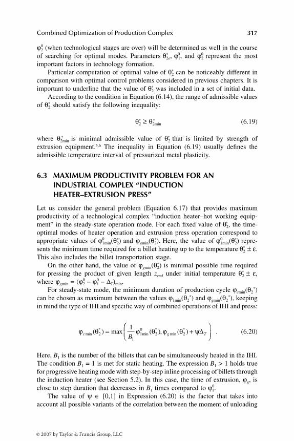
Combined Optimization of Production Complex 317
ϕ20 (when technological stages are over) will be determined as well in the course
of searching for optimal modes. Parameters *θ2e,0ϕ1, and ϕ2
0 represent the mostimportant factors in technology formation.
Particular computation of optimal value of θ2* can be noticeably different in
comparison with optimal control problems considered in previous chapters. It isimportant to underline that the value of θ2
* was included in a set of initial data. According to the condition in Equation (6.14), the range of admissible values
of θ2* should satisfy the following inequality:
*θ2 ≥ *θ2min (6.19)
where θ2min* is minimal admissible value of θ2
* that is limited by strength ofextrusion equipment.5,6 The inequality in Equation (6.19) usually defines theadmissible temperature interval of pressurized metal plasticity.
6.3 MAXIMUM PRODUCTIVITY PROBLEM FOR AN INDUSTRIAL COMPLEX “INDUCTION HEATER–EXTRUSION PRESS”
Let us consider the general problem (Equation 6.17) that provides maximumproductivity of a technological complex “induction heater–hot working equip-ment” in the steady-state operation mode. For each fixed value of *θ2, the time-optimal modes of heater operation and extrusion press operation correspond toappropriate values of 0ϕ1min(θ2)* and ϕgmin(θ2).* Here, the value of 0ϕ1min(θ2)* repre-sents the minimum time required for a billet heating up to the temperature θ2
* ± ε.This also includes the billet transportation stage.
On the other hand, the value of ϕgmin(θ2)* is minimal possible time requiredfor pressing the product of given length zend under initial temperature θ2
* ± ε,where ϕgmin = (ϕ2
0 – ϕ10 – ∆T)min.
For steady-state mode, the minimum duration of production cycle ϕcmin(θ2*)
can be chosen as maximum between the values ϕ1min(θ2*) and ϕgmin(θ2
*), keepingin mind the type of IHI and specific way of combined operations of IHI and press:
. (6.20)
Here, B1 is the number of the billets that can be simultaneously heated in the IHI.The condition B1 = 1 is met for static heating. The expression B1 > 1 holds truefor progressive heating mode with step-by-step inline processing of billets throughthe induction heater (see Section 5.2). In this case, the time of extrusion, ϕg, isclose to step duration that decreases in B1 times compared to 0ϕ1.
The value of ψ ∈ [0,1] in Expression (6.20) is the factor that takes intoaccount all possible variants of the correlation between the moment of unloading
ϕ θ ϕ θ ϕ θ ψc g TBmin*
min*
min*( ) max ( ), ( )2
110
2 2
1= + ∆
DK6039_C006.fm Page 317 Thursday, June 8, 2006 3:14 PM
© 2007 by Taylor & Francis Group, LLC

318 Optimal Control of Induction Heating Processes
of the next billet and completion of the previous billet pressing. If a heated billetexits an induction heater after complete unloading of the press product, then ψ= 1 and IHI output rate should be close to the sum ϕg + ∆T . In this case, the idletime of press equipment during one cycle always turns out to be not less thanbillet transportation time.
If there is no interaction between these operations, then unloading of billetscould be performed regardless of press operational mode and billets could bedelivered to press with the rate equal to IHI output rate. In this case, the valueof ϕg would be close to the value of 0ϕ1/B1 and ψ = 0. Intermediate variants takeplace under condition of 0 < ψ < 1.
Obviously, the minimum value ϕcmin(θ2)* is the optimal duration of the pro-duction cycle ϕc
* that provides maximum possible productivity of the technolog-ical complex “induction heater–extrusion press.” Therefore, according to Equa-tion (6.20), it is possible to write:
.
(6.21)
If the functions 0ϕ1min(θ2)* and ϕgmin(θ2)* are known, the optimal temperatureprofile at the end of heating stage can be defined from Expression (6.21) asfollows:
. (6.22)
This value corresponds to the optimal duration, *ϕc , of the production cycle;therefore, the value of ϕc
* can be defined as well. When the value of θ2e* is found,
it is possible to perform the valid decomposition of the joint maximum produc-tivity optimization problem of induction heater and extrusion press.
Decomposition is reduced to statement of the maximum productivity problemfor the cycle stage, which duration is longer, under the condition of θ2
* = *θ2e. Thismeans that, to reduce the value of ϕc
* (see Expression 6.21), the technologicalstage with a maximum duration should be optimized with respect to the time-optimal criterion. The technological stage that has the shortest duration shouldbe optimized with respect to a cost function of the type in Equation (6.18).
The functions 0ϕ1min(θ2)* and ϕgmin(θ2)* should be defined as a result of solutionsof separate local time-optimal control problems for heating process and billetextrusion. A sequence of optimization problems should be solved for fixed valuesθ2
* that satisfy the condition in Equation (6.19). The first problem can be solvedby methods described in previous chapters, but the second one represents anindependent problem and requires special consideration. Section 6.5 discussesseveral possible ways of finding the required solution.5
ϕ ϕ θθ θ θ θ
c c*
min*min min ma
*min
* *min
*= ( ) =
≥ ≥2 2 2 22 xx ,min
*min
*1
110
2 2B
g Tϕ θ ϕ θ ψ( ) ( ) +
∆
θ ϕ θ ϕθ θ
21
10
22 2
1e g
B*
min*
miarg min max ,*
min*
= ( )≥
nn*θ ψ2( ) +
∆T
DK6039_C006.fm Page 318 Thursday, June 8, 2006 3:14 PM
© 2007 by Taylor & Francis Group, LLC

Combined Optimization of Production Complex 319
Figure 6.1 shows all possible cases that could take place when solving theproblem in Equation (6.21) and Equation (6.22) with respect to different variantsof relations between minimal durations of billet heating and pressing processesunder considered temperature range of *θ2 variation.
The value 0ϕ1min increases monotonously with θ2* growth and the curve
ϕgmin(θ2)* has an evident extremum. Minimum of ϕgmin(θ2)* is reached at the tem-perature θ2
* = *θ2c. Growth of ϕgmin(θ2)* under θ2* < θ2c
* occurs due to a reduction ofmaximal velocity of extrusion for the press hydraulic drive because pressing forceincreases with billet temperature reduction.11 A similar effect under θ2
* > θ2c* can
be explained by forced reduction of pressing velocity under the restraint inEquation (6.13).10 Figure 6.1a shows the case when the expression ϕgmin(θ2)* +ψ∆T > ϕ1min
0 (θ2)/B1* is valid for all values θ2
* ≥ *θ2min. The maximum productivityof complex is limited by only technical limitations of extrusion press for the
FIGURE 6.1 Minimal durations of billet heating and hot forming processes as functionsof temperature at the end of heating. a–c: For complex “induction heating–extrusionoperation”; d: for complex “induction heating–rolling operation”; 1: ϕgmin + ψ∆T;2: ϕ1min/B1.
0
0
A2
C2
P2
F2
D2
D2
1
2
0
(a) (b)
(c) (d)
A C
P
F
1
ϕ
ϕ ϕ
ϕ
θ∗2c
θ∗2 min
θ∗2
θ∗2c
θ∗2 min
θ∗2 min
θ∗2
θ∗2eθ∗
2cθ∗
2 minθ∗
2 minθ∗
2θ∗
2 endθ∗
2
2
1
2
0
A1 C1
C 1
P
D1
D 1
1
2
F1
DK6039_C006.fm Page 319 Thursday, June 8, 2006 3:14 PM
© 2007 by Taylor & Francis Group, LLC
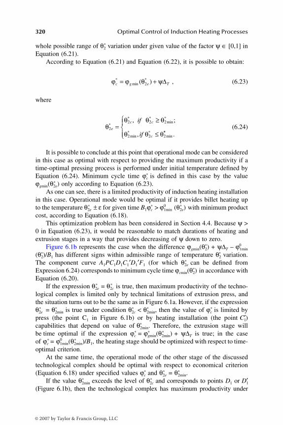
320 Optimal Control of Induction Heating Processes
whole possible range of θ2* variation under given value of the factor ψ ∈ [0,1] in
Equation (6.21).According to Equation (6.21) and Equation (6.22), it is possible to obtain:
, (6.23)
where
(6.24)
It is possible to conclude at this point that operational mode can be consideredin this case as optimal with respect to providing the maximum productivity if atime-optimal pressing process is performed under initial temperature defined byEquation (6.24). Minimum cycle time ϕc
* is defined in this case by the valueϕgmin(θ2e)* only according to Equation (6.23).
As one can see, there is a limited productivity of induction heating installationin this case. Operational mode would be optimal if it provides billet heating upto the temperature θ2e
* ± ε for given time B1ϕc* > ϕ1min
0 (θ2e)* with minimum productcost, according to Equation (6.18).
This optimization problem has been considered in Section 4.4. Because ψ >0 in Equation (6.23), it would be reasonable to match durations of heating andextrusion stages in a way that provides decreasing of ψ down to zero.
Figure 6.1b represents the case when the difference ϕgmin(θ2)* + ψ∆T –0ϕ1min
(θ2)/B1* has different signs within admissible range of temperature θ2
* variation.The component curve A1PC1D1C1′D1′F1 (for which θ2e
* can be defined fromExpression 6.24) corresponds to minimum cycle time ϕcmin(θ2)* in accordance withEquation (6.20).
If the expression θ2e* = θ2c
* is true, then maximum productivity of the techno-logical complex is limited only by technical limitations of extrusion press, andthe situation turns out to be the same as in Figure 6.1a. However, if the expressionθ2e
* = θ2min* is true under condition θ2c
* < *θ2min, then the value of ϕc* is limited by
press (the point C1 in Figure 6.1b) or by heating installation (the point 1C′)capabilities that depend on value of *θ2min. Therefore, the extrusion stage willbe time optimal if the expression ϕc
* = *ϕgmin(θ2min)* + ψ∆T is true; in the caseof *ϕc =
0ϕ1min(θ2min)/B1,* the heating stage should be optimized with respect to time-optimal criterion.
At the same time, the operational mode of the other stage of the discussedtechnological complex should be optimal with respect to economical criterion(Equation 6.18) under specified values ϕc
* and θ2e* = *θ2min.
If the value θ2min* exceeds the level of θ2c
* and corresponds to points D1 or 1D′(Figure 6.1b), then the technological complex has maximum productivity under
ϕ ϕ θ ψc g e T*
min*( )= +2 ∆
θθ θ θ
θ θ θ2
2 2 2
2 2 2
e
c c
c
if
if
*
* *min
*
min* *
min
, ;
,=
≥
≤ ** .
DK6039_C006.fm Page 320 Thursday, June 8, 2006 3:14 PM
© 2007 by Taylor & Francis Group, LLC

Combined Optimization of Production Complex 321
time-optimal control of operational mode for heating and extrusion stages. Thismeans that maximum productivity of the technological complex can be providedonly if both heater and hot working equipment operate with maximum productivity.
Figure 6.1c shows the case that differs from the previous one. Here, maximumpress productivity under θ2
* = θ2c* cannot be reached because of insufficient output
rate of the heating installation under the condition:
.
Component curve A2D2C2D2′F2 corresponds to the value *ϕcmin(θ2c)* (seeExpression 6.20) and defines the value of θ2e
* in the point D2 (in accordance withExpression 6.22). If the restraint (Equation 6.19) is not violated in this point,then the following equation can be written:
(6.25)
under time-optimal control of pressing and heating processes. Otherwise, thesituation is similar to the one shown in Figure 6.1b.
In all cases, the value of θ2e* can be found according to Expression (6.22). At
the same time, ϕc* could be found using the algorithm in Equation (6.21), and
optimal durations of the heating 0(ϕ1opt) and pressing 0(ϕg opt) processes can becomputed according to the following correlations:
(6.26)
The optimal control problem could be solved in a similar way with respectto maximal productivity of the technological complex that consists of anothertype of metal working operation — for example, for the technological complex“induction heating–rolling operation.”
In case of optimizing the “induction heating–rolling” system, the dependencyϕgmin(θ2)* has* a monotonous decreasing nature12 and it is possible to obtain thecondition shown in Figure 6.1d that is similar to the case considered previouslyin Figure 6.1c for the point D2. If minimum production cost (Equation 6.18) is
ϕ θ ϕ θ ψ10
2 1 2min*
min*( ) / ( )c g c TB > + ∆
ϕ θ ϕ θ ψmin*
min*( ) / ( )0
2 1 2e g e TB = + ∆
ϕϕ θ ϕ ϕ θ
10
10
21
10
21
opt ==min
* *min
*( ), ( );e c eifB
B11 2 2ϕ θ ψ ϕ ϕ θ ψg e T c g e Tifmin* *
min*( ) , ( )+ = +∆ ∆ ;;
( ), (min* *
min*
==
ϕϕ θ ϕ ϕ θ
g
g e c g eif
opt
2 2 )) ;
( ) , (min* *
min
+
− =
ψ
ϕ θ ψ ϕ ϕ
∆
∆
T
e T cB
ifB
1 1
110
21
10 θθ2e
* ).
DK6039_C006.fm Page 321 Thursday, June 8, 2006 3:14 PM
© 2007 by Taylor & Francis Group, LLC

322 Optimal Control of Induction Heating Processes
required for the technological complex “heating–extrusion,” then the joint opti-mization problem could be solved by using the same technique as for maximumproductivity problem.
Instead of dependencies 0ϕ1min(θ2)* and ϕgmin(θ2)* in Equation (6.21) and assum-ing that the values ϕ1
0 and ϕg are given, it would be necessary to find separatevalues for heating (I2Hmin (θ2))* and for extrusion (I2gmin(θ2))* that correspond tominimum expenses in the form of appropriate items of the sum (Equation 6.18).These values can be found by solving the appropriate local optimization problemsunder fixed values *θ2.
For each fixed value of θ2,* the minimal value of production cost I2min(θ2)* canbe considered as the sum of expenses for heating and extrusion (according toEquation 6.18). Thus, the following minimization procedure with respect to *θ2
defines optimal value I2 = I2* in accordance with the algorithm of Equation (6.21):
. (6.27)
It should be pointed out here that, similarly to the case of solving the maximumproductivity problem, it is possible to find optimal value θ2e
* that represents aninitial extrusion temperature as follows:
. (6.28)
6.4 MULTIPARAMETER STATEMENT OF THE OPTIMIZATION PROBLEM FOR TECHNOLOGICAL COMPLEX “HEATING–HOT FORMING”
Solution of the problem that provides maximum productivity of the technologicalcomplex “induction heater–hot working equipment” (Section 6.3) is based onconsideration of all possible initial temperature states of metal prior to hot formingin the class of one-parameter functions. The temperature θ2
* uniformly distributedwithin the billet with a priori fixed absolute inaccuracy ε can be considered asthe single parameter.
Such an approach can be extended to more complex problems of combinedoptimization of the technological complex “heating–hot forming” when temper-ature profiles of treated billets are given in the parametric form as a function oftwo and more parameters. Heating accuracy ε can be considered as an exampleof these parameters. Optimal values εe and θ2e
* should be determined in the courseof searching optimal control functions. The value εe can be included in the setof technological parameters within process flow sheets that should be optimized.
I I I2 2 2 22 2 2 2
*min
*min ( ) min*
min* *
min*
= =≥ ≥θ θ θ θ
θ HH gImin*
min*( ) ( )θ θ2 2 2+
θ θ θθ θ
2 2 2 2 22 2
e H gI I*min
*minarg min ( ) (
*min
*= +
≥
** )
DK6039_C006.fm Page 322 Thursday, June 8, 2006 3:14 PM
© 2007 by Taylor & Francis Group, LLC
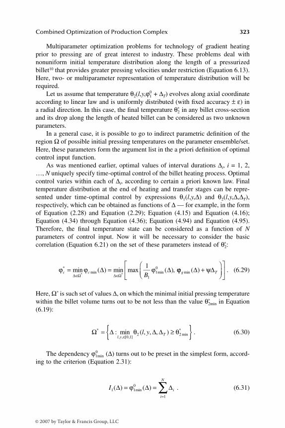
Combined Optimization of Production Complex 323
Multiparameter optimization problems for technology of gradient heatingprior to pressing are of great interest to industry. These problems deal withnonuniform initial temperature distribution along the length of a pressurizedbillet10 that provides greater pressing velocities under restriction (Equation 6.13).Here, two- or multiparameter representation of temperature distribution will berequired.
Let us assume that temperature θ2(l,y,ϕ10 + ∆T) evolves along axial coordinate
according to linear law and is uniformly distributed (with fixed accuracy ± ε) ina radial direction. In this case, the final temperature θ2
* in any billet cross-sectionand its drop along the length of heated billet can be considered as two unknownparameters.
In a general case, it is possible to go to indirect parametric definition of theregion Ω of possible initial pressing temperatures on the parameter ensemble/set.Here, these parameters form the argument list in the a priori definition of optimalcontrol input function.
As was mentioned earlier, optimal values of interval durations ∆i, i = 1, 2,…, N uniquely specify time-optimal control of the billet heating process. Optimalcontrol varies within each of ∆i, according to certain a priori known law. Finaltemperature distribution at the end of heating and transfer stages can be repre-sented under time-optimal control by expressions θ1(l,y,∆) and θ2(l,y,∆,∆T),respectively, which can be obtained as functions of ∆ — for example, in the formof Equation (2.28) and Equation (2.29); Equation (4.15) and Equation (4.16);Equation (4.34) through Equation (4.36); Equation (4.94) and Equation (4.95).Therefore, the final temperature state can be considered as a function of Nparameters of control input. Now it will be necessary to consider the basiccorrelation (Equation 6.21) on the set of these parameters instead of *θ2:
. (6.29)
Here, Ω* is such set of values ∆, on which the minimal initial pressing temperaturewithin the billet volume turns out to be not less than the value θ2min
* in Equation(6.19):
. (6.30)
The dependency ϕ1min0 (∆) turns out to be preset in the simplest form, accord-
ing to the criterion (Equation 2.31):
. (6.31)
ϕ ϕ ϕc c B*
min minmin ( ) min max ( ),* *
= =∈ ∈∆ Ω ∆ Ω
∆ ∆1
110 ϕϕ ψg Tmin ( )∆ ∆+
Ω ∆ ∆ ∆*
, , [ , ]min
*: min ( , , , )= ≥ ∈l yTl y
0 12 2θ θ
I i
i
N
1 10
1
( ) ( )min∆ ∆ ∆= ==∑ϕ
DK6039_C006.fm Page 323 Thursday, June 8, 2006 3:14 PM
© 2007 by Taylor & Francis Group, LLC

324 Optimal Control of Induction Heating Processes
Therefore, only the function ϕgmin(∆) should be found by solving the time-optimal problem for the pressing process with respect to an admissible set (Equa-tion 6.30) of fixed values ∆. These values uniquely define initial temperature stateθ3(l,y,ϕ1
0 + ∆T) ≡ θ2(l,y,∆,∆T) of a pressurized billet. As a result, similarly to *θ2e
in Equation (6.22), extremum values ∆ie, i = 1, 2, …, N could be defined. Underthese values, Expression (6.29) holds true for *ϕc. Optimal temperature state *θ20pt
(l,* y, ∆e, ∆T) corresponds to values ∆ie, i = 1, 2, …, N.The described method of parametric assignment of the initial pressing tem-
peratures set in general does not predestine the shape of spatial temperaturedistribution within the billet volume during the pressing process. Therefore, dueto extension of the region Ω in Equation (6.14) (in comparison with the conditionin Equation 6.19), the choice of temperature states can be performed more freely,and the value of combined cost function for the technological complex optimi-zation can be improved.
At the same time, a multidimensional search procedure with respect to values∆ie, i = 1, 2, …, N that is performed according to algorithm (Equation 6.29) willbe more complicated in comparison with the one-dimensional case (Equation6.21).
When minimum product cost of the technological complex is required, asimilar optimization problem can be formulated with respect to set of parameters∆ = (∆(1),∆(2)) that specify optimal control of heating (∆(1)) and pressing (∆(2))processes. Here, ∆(1) and ∆(2) could make another physical sense in comparisonwith parameter vector ∆ in Expression (6.29). Because the value ∆(1) uniquelyspecifies temperature distribution θ2(l,y,∆(1),∆T), and, in the same time, criterionI2g depends on this temperature distribution, ∆(2) incorporates the components ofvector ∆(1). As a result, similarly to Equation (6.29), the expression for I2
* can beobtained instead of Equation (6.27) in the following form:
. (6.32)
Here, Ω1* can be defined similarly to Equation (6.30), and Ω2
* can be foundaccording to restriction (Equation 6.13) as follows:
(6.33)
where θ3(lk,1,∆(2),ϕ) represents the temperature in the die hole (l = lk, y = 1) atany time ϕ during the pressing process for each fixed value of the vector ∆(2).
I I2 21 2
11
22
*
,
( ) ( )min ( , ) min( ) * ( ) * (
= =∈ ∈∆ Ω ∆ Ω ∆
∆ ∆11
12
22
12
2) * ( ) *,
( ) ( )( ) ( )∈ ∈
+ Ω ∆ Ω∆ ∆I IH g
Ω ∆ ∆ ∆11
0 12
12
* ( )
, [ , ]
( )min
*: min ( , , , )= ≥∈l y
Tl yθ θ = ≤ + ≤ ≤
;
: ( , , , ) ,* ( ) ( )Ω ∆ ∆ ∆22
32
3 101θ ϕ θ ϕ ϕlk cr T ϕϕ2
0
,
DK6039_C006.fm Page 324 Thursday, June 8, 2006 3:14 PM
© 2007 by Taylor & Francis Group, LLC
Combined Optimization of Production Complex 325
6.5 COMBINED OPTIMIZATION OF HEATING AND PRESSING MODES FOR ALUMINUM ALLOY BILLETS
The described method has been used for analysis of productivity of the techno-logical complex for heating of aluminum alloy D16 cylindrical billets and theirsubsequent hot forming on the horizontal hydraulic press. Length of the billet is350 mm; applied frequency is 50 Hz; diameter of the press product (rods) is 22mm; and diameter of the press container is 90 mm.5,6 Technological requirementdemands that required uniformity of temperature distribution within the billetshould be provided prior to the hot forming operation.
At the first step, local problems of time-optimal control should be solvedseparately for heating and pressing processes. It is important to note that herethe given set of permissible values of initial pressurized metal temperatures *θ2
should be taken into account. At the next step, the minimum duration of produc-tion cycle should be chosen according to the condition in Equation (6.20).
6.5.1 TIME-OPTIMAL HEATING MODES
Dependency 0ϕ1min(θ2)* can be obtained with regard to models (Equation 6.1through Equation 6.6) by using techniques described in Chapter 3 and Chapter4. Restraint on maximum temperature at the level of 500° should be taken intoaccount. Maximum value of heating power (that is uniformly distributed alongthe billet length) is equal to 60 kW/m2.
Heat losses from the billet surface during heating and transfer stages (∆T =30 s) can be estimated by values of Bih = 0.015 and BiT = 0.030, respectively, inboundary conditions in Equation (6.2) and Equation (6.5). It is assumed that theexpression ∆T > ∆T2
* (Section 4.2) holds true.Calculations have been conducted for several fixed values of final heating
temperatures θ2* in the range of 320 to 470° under required accuracy ε = .
Here, the lower value, θ2min* = 320°, in Equation (6.19) is in agreement with
requirements to press instrument strength, and the upper value of 480° representsthe maximum permissible temperature in the die hole, according to the conditionin Equation (6.13).
Calculated values do not exceed 5°C and practically do not depend onthe value θ2
* in the considered temperature range. This fact allows obtaining theexpression θ2(l,y,ϕ1
0 + ∆T) ≅ θ2* = const that holds true with acceptable accuracy.
This expression can be used in order to define temperature distribution duringthe pressing process.
6.5.2 TIME-OPTIMAL PRESSING MODES
Dependency ϕg min (θ2)* in Equation (6.21) can be defined after solving the localtime-optimal problem for the pressing process. The fixed values of initial billettemperatures prior to hot forming operation should be considered within the range
εmin( )2
εmin( )2
DK6039_C006.fm Page 325 Thursday, June 8, 2006 3:14 PM
© 2007 by Taylor & Francis Group, LLC
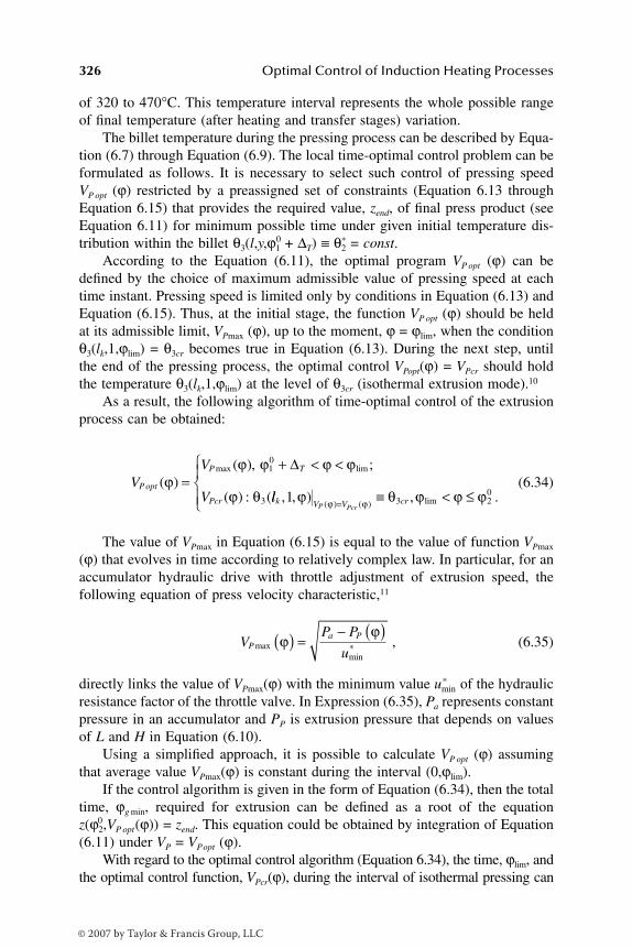
326 Optimal Control of Induction Heating Processes
of 320 to 470°C. This temperature interval represents the whole possible rangeof final temperature (after heating and transfer stages) variation.
The billet temperature during the pressing process can be described by Equa-tion (6.7) through Equation (6.9). The local time-optimal control problem can beformulated as follows. It is necessary to select such control of pressing speedVP opt (ϕ) restricted by a preassigned set of constraints (Equation 6.13 throughEquation 6.15) that provides the required value, zend, of final press product (seeEquation 6.11) for minimum possible time under given initial temperature dis-tribution within the billet θ3(l,y,ϕ1
0 + ∆T) ≡ θ2* = const.
According to the Equation (6.11), the optimal program VP opt (ϕ) can bedefined by the choice of maximum admissible value of pressing speed at eachtime instant. Pressing speed is limited only by conditions in Equation (6.13) andEquation (6.15). Thus, at the initial stage, the function VP opt (ϕ) should be heldat its admissible limit, VPmax (ϕ), up to the moment, ϕ = ϕlim, when the conditionθ3(lk,1,ϕlim) = θ3cr becomes true in Equation (6.13). During the next step, untilthe end of the pressing process, the optimal control VPopt(ϕ) = VPcr should holdthe temperature θ3(lk,1,ϕlim) at the level of θ3cr (isothermal extrusion mode).10
As a result, the following algorithm of time-optimal control of the extrusionprocess can be obtained:
(6.34)
The value of VPmax in Equation (6.15) is equal to the value of function VPmax
(ϕ) that evolves in time according to relatively complex law. In particular, for anaccumulator hydraulic drive with throttle adjustment of extrusion speed, thefollowing equation of press velocity characteristic,11
, (6.35)
directly links the value of VPmax(ϕ) with the minimum value umin* of the hydraulic
resistance factor of the throttle valve. In Expression (6.35), Pa represents constantpressure in an accumulator and PP is extrusion pressure that depends on valuesof L and H in Equation (6.10).
Using a simplified approach, it is possible to calculate VP opt (ϕ) assumingthat average value VPmax(ϕ) is constant during the interval (0,ϕlim).
If the control algorithm is given in the form of Equation (6.34), then the totaltime, ϕg min, required for extrusion can be defined as a root of the equationz(ϕ2,VP opt(ϕ))0 = zend. This equation could be obtained by integration of Equation(6.11) under VP = VPopt (ϕ).
With regard to the optimal control algorithm (Equation 6.34), the time, ϕlim, andthe optimal control function, VPcr(ϕ), during the interval of isothermal pressing can
VV
VP opt
P T
Pcr
( )( ), ;
( ) : (
max lim
ϕϕ ϕ ϕ ϕ
ϕ θ=
+ < <10
3
∆
llk V V crP Pcr
, , ) , .( ) ( ) lim1 3 2
0ϕ θ ϕ ϕ ϕϕ ϕ= ≡ < ≤
VP P
uP
a Pmax
min*ϕ
ϕ( ) = − ( )
DK6039_C006.fm Page 326 Thursday, June 8, 2006 3:14 PM
© 2007 by Taylor & Francis Group, LLC
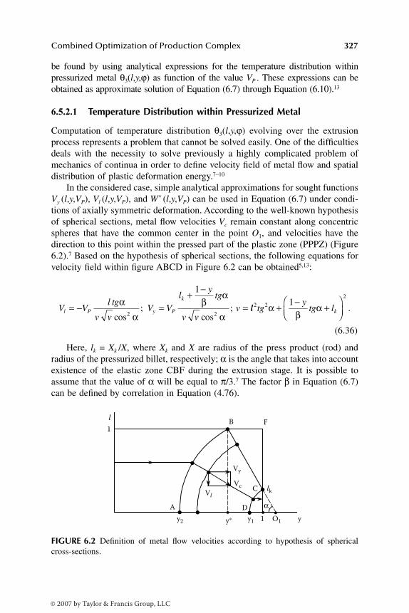
Combined Optimization of Production Complex 327
be found by using analytical expressions for the temperature distribution withinpressurized metal θ3(l,y,ϕ) as function of the value VP . These expressions can beobtained as approximate solution of Equation (6.7) through Equation (6.10).13
6.5.2.1 Temperature Distribution within Pressurized Metal
Computation of temperature distribution θ3(l,y,ϕ) evolving over the extrusionprocess represents a problem that cannot be solved easily. One of the difficultiesdeals with the necessity to solve previously a highly complicated problem ofmechanics of continua in order to define velocity field of metal flow and spatialdistribution of plastic deformation energy.7–10
In the considered case, simple analytical approximations for sought functionsVy (l,y,VP), Vl (l,y,VP), and W* (l,y,VP) can be used in Equation (6.7) under condi-tions of axially symmetric deformation. According to the well-known hypothesisof spherical sections, metal flow velocities Vc remain constant along concentricspheres that have the common center in the point O1, and velocities have thedirection to this point within the pressed part of the plastic zone (PPPZ) (Figure6.2).7 Based on the hypothesis of spherical sections, the following equations forvelocity field within figure ABCD in Figure 6.2 can be obtained5,13:
(6.36)
Here, lk = Xk /X, where Xk and X are radius of the press product (rod) andradius of the pressurized billet, respectively; α is the angle that takes into accountexistence of the elastic zone CBF during the extrusion stage. It is possible toassume that the value of α will be equal to π/3.7 The factor β in Equation (6.7)can be defined by correlation in Equation (4.76).
FIGURE 6.2 Definition of metal flow velocities according to hypothesis of sphericalcross-sections.
V Vl tg
v vV V
ly
tg
v vvl P y P
k
= − =+ −
=αα
βα
αcos;
cos;
2 2
1
ll tgy
tg lk2 2
21α
βα+ − +
.
lk
Vy
Vc
Vl
1
l
yy2 y1y∗
α
1 O1
C
B
A D
F
DK6039_C006.fm Page 327 Thursday, June 8, 2006 3:14 PM
© 2007 by Taylor & Francis Group, LLC
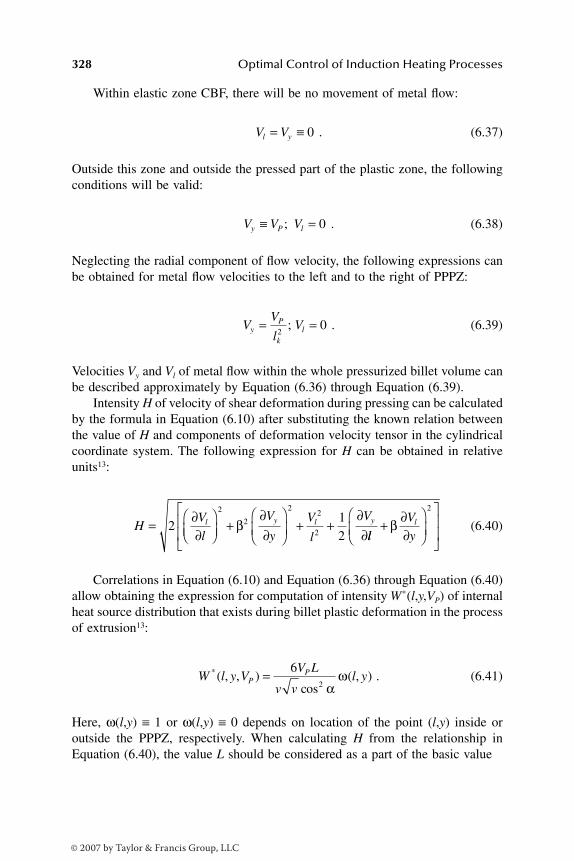
328 Optimal Control of Induction Heating Processes
Within elastic zone CBF, there will be no movement of metal flow:
. (6.37)
Outside this zone and outside the pressed part of the plastic zone, the followingconditions will be valid:
. (6.38)
Neglecting the radial component of flow velocity, the following expressions canbe obtained for metal flow velocities to the left and to the right of PPPZ:
. (6.39)
Velocities Vy and Vl of metal flow within the whole pressurized billet volume canbe described approximately by Equation (6.36) through Equation (6.39).
Intensity H of velocity of shear deformation during pressing can be calculatedby the formula in Equation (6.10) after substituting the known relation betweenthe value of H and components of deformation velocity tensor in the cylindricalcoordinate system. The following expression for H can be obtained in relativeunits13:
(6.40)
Correlations in Equation (6.10) and Equation (6.36) through Equation (6.40)allow obtaining the expression for computation of intensity W*(l,y,VP) of internalheat source distribution that exists during billet plastic deformation in the processof extrusion13:
. (6.41)
Here, ω(l,y) ≡ 1 or ω(l,y) ≡ 0 depends on location of the point (l,y) inside oroutside the PPPZ, respectively. When calculating H from the relationship inEquation (6.40), the value L should be considered as a part of the basic value
V Vl y= ≡ 0
V V Vy P l≡ =; 0
VV
lVy
P
kl= =
20;
HV
l
V
y
V
l
Vl y l y= ∂
∂
+∂∂
+ +
∂∂
212
2
2
22
2β
ll
V
yl+ ∂
∂
β2
W l y VV L
v vl yP
P* ( , , )cos
( , )= 62 α
ω
DK6039_C006.fm Page 328 Thursday, June 8, 2006 3:14 PM
© 2007 by Taylor & Francis Group, LLC

Combined Optimization of Production Complex 329
.
In Expression (6.41), it is reasonable to use linear approximation of thefunction L(θ)10 as follows:
, (6.42)
where T0 corresponds to value of T under basic temperature, and Kθ is the constantfactor.
Let us assume that heat flow density of contact friction q(y,VP) in the boundarycondition in Equation (6.8) is proportional to velocity Vy(l,y) at the billet surfacel = 1.14 In this case, the following correlation can be obtained, taking into accountExpression (6.37) and Expression (6.38):
(6.43)
Here, Kq = const is coefficient of proportionality.Analytical solution of heat transfer problems in Equation (6.7) through Equa-
tion (6.10) with respect to temperature distribution θ3(l,y,ϕ) will be greatly com-plicated due to highly pronounced nonuniformity of spatial distribution of metalflow velocities. This is so even in the case when simplified Expression (6.37)through Expression (6.43) represent explicit functions Vl , Vy , W*, and q fromtheir arguments.
A simplified approach provided in Rapoport13 allows one to solve the problemfor initial and steady-state stages of extrusion with constant speed VP = const.The numerical model that describes temperature distribution θ3(l,y,ϕ) during avariety of hot forming processes15 can be successfully applied to optimization ofdifferent modes of a hot forming operation. This numerical model has beenobtained in the course of the problem (Equation 6.7 through Equation 6.10)solution by using the finite-difference method under conditions in Equation (6.37)through Equation (6.43).
6.5.2.2 Optimal Program of Extrusion Speed Variation
In the considered case, the constant averaged value of extrusion speed is equalto VPmax ≅ 5 m/min during the interval (ϕ1
0 + ∆T , ϕlim). The correlation θ2c* < *θ2min
(Figure 6.1) will be valid for each time point that belongs to the interval (ϕ10 +
∆T , ϕlim). The value ϕlim should be defined as the moment when maximumpermissible temperature θ3cr = θ3(lk,1,ϕlim) in the die hole is reached. Under
LW X
Vbb
b
=*
L T K( )θ θθ= −0
q y V
K V y y
y y ytg
lP
q P
k
( , )
, ;
, ; (
*
* *=
≤ ≤
< ≤ = − −
0
0 1 1 1βα
)).
DK6039_C006.fm Page 329 Thursday, June 8, 2006 3:14 PM
© 2007 by Taylor & Francis Group, LLC
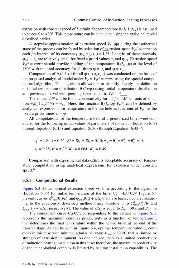
330 Optimal Control of Induction Heating Processes
extrusion with constant speed of 5 m/min, the temperature θ3(lk ,1,ϕlim) is assumedto be equal to 480°. This temperature can be calculated using the analytical modeldescribed earlier.
A stepwise approximation of extrusion speed VPcr(ϕ) during the isothermalstage of the process can be found by selection of extrusion speed VP
(j) = const oneach jth interval of its constancy . Lengths of these intervals,ϕj+1 – ϕj, are relatively small for fixed a priori values ϕj and ϕj+1. Extrusion speedVP
(j) = const should provide holding of the temperature θ3(lk,1,ϕ) at the level of480° with required accuracy for all times ϕ = ϕj and ϕ = ϕj+1.
Computation of θ3(lk,1,ϕ) for all ϕ ∈ (ϕj,ϕj+1) was conducted on the basis ofthe proposed analytical model under VP = VP
(j) = const using the special compu-tational algorithm. This algorithm allows one to simplify sharply the definitionof initial temperature distribution θ3(l,y,ϕj) using initial temperature distributionat a previous interval with pressing speed equal to VP
(j–1).16
The values VP(j) can be found consecutively for all as roots of equa-
tion θ3(lk,1,ϕj,VP(j)) = θ3cr . Here, the function θ3(lk,1,ϕj,VP
(j)) can be defined byanalytical expressions for temperature in the die hole as functions of VP
(j) at thefixed a priori times ϕ = ϕj.
All computations for the temperature field of a pressurized billet were con-ducted for the following initial values of parameters of models in Equation (6.7)through Equation (6.15) and Equation (6.36) through Equation (6.43)13:
Comparison with experimental data exhibits acceptable accuracy of temper-ature computation using analytical expressions for extrusion under constantspeed.16
6.5.3 Computational Results
Figure 6.3 shows optimal extrusion speed vs. time according to the algorithm(Equation 6.34) for initial temperature of the billet θ2
* = 450°C.5,6 Figure 6.4presents curves 0ϕ1min(θ2)/B1
* and ϕgmin(θ2)* + ψ∆T that have been calculated accord-ing to the previously described method using absolute units 0(τ1min(t2)/B1
* andτgmin(t2)* + ψ∆T , respectively). The value of ψ∆T is equal to ∆T = 30 s and B1 = 3.
The component curve C2D2′F2 corresponding to the variant in Figure 6.1crepresents the maximum complex productivity as a function of temperature *t2
that determines the final temperature within the heated billet at the end of thetransfer stage. As can be seen in Figure 6.4, optimal temperature value *t2e coin-cides in this case with minimal admissible value t2min
* = 320°C that is limited bystrength of extrusion equipment. As one can see, there is a limited productivityof induction heating installation in this case; therefore, the maximum productivityof the technological complex is limited by heating installation capabilities. The
( , ), ,ϕ ϕj j j M+ =1 1
j M= 1,
γ β θ θ θ θ* . ; . ; . ;= = = = = = = =1 8 0 26 0 150 10 0
0Bi Bi Bi a a a aa
l K Kk q
10 0
0 25 3 0 064 0 49
=
= = = =
;
. ; / ; . ; . .α π θ
DK6039_C006.fm Page 330 Thursday, June 8, 2006 3:14 PM
© 2007 by Taylor & Francis Group, LLC

Combined Optimization of Production Complex 331
FIGURE 6.3 Optimal pressing velocity vs. time.
FIGURE 6.4 Minimal durations of billet heating and pressing processes as functions oftemperature at the end of heating.
0
0.2
0.4
0.6
0.8
1.2
1.0
5 15 25 35 45 τ, s
mm/min,125
VP
VP st
VP
0
2
4
6
8
10
τ, min
τ∗c
τ01 min
/3
τ01 min
/5
300 340 380 420 460
C2
F2
D′2
τg min + ∆T
t∗2 min
= t∗2e
t∗2, °C
t∗2p
DK6039_C006.fm Page 331 Thursday, June 8, 2006 3:14 PM
© 2007 by Taylor & Francis Group, LLC
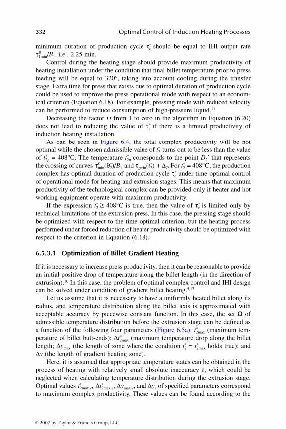
332 Optimal Control of Induction Heating Processes
minimum duration of production cycle τc* should be equal to IHI output rate
τ1min/B1,0 i.e., 2.25 min.
Control during the heating stage should provide maximum productivity ofheating installation under the condition that final billet temperature prior to pressfeeding will be equal to 320°, taking into account cooling during the transferstage. Extra time for press that exists due to optimal duration of production cyclecould be used to improve the press operational mode with respect to an econom-ical criterion (Equation 6.18). For example, pressing mode with reduced velocitycan be performed to reduce consumption of high-pressure liquid.11
Decreasing the factor ψ from 1 to zero in the algorithm in Equation (6.20)does not lead to reducing the value of τc
* if there is a limited productivity ofinduction heating installation.
As can be seen in Figure 6.4, the total complex productivity will be notoptimal while the chosen admissible value of t2
* turns out to be less than the valueof t2p
* = 408°C. The temperature t2p* corresponds to the point D2′ that represents
the crossing of curves 0τmin(θ2)/B1* and τgmin(t2)* + ∆T. For t2
* = 408°C, the productioncomplex has optimal duration of production cycle τc
* under time-optimal controlof operational mode for heating and extrusion stages. This means that maximumproductivity of the technological complex can be provided only if heater and hotworking equipment operate with maximum productivity.
If the expression t2* ≥ 408°C is true, then the value of τc
* is limited only bytechnical limitations of the extrusion press. In this case, the pressing stage shouldbe optimized with respect to the time-optimal criterion, but the heating processperformed under forced reduction of heater productivity should be optimized withrespect to the criterion in Equation (6.18).
6.5.3.1 Optimization of Billet Gradient Heating
If it is necessary to increase press productivity, then it can be reasonable to providean initial positive drop of temperature along the billet length (in the direction ofextrusion).10 In this case, the problem of optimal complex control and IHI designcan be solved under condition of gradient billet heating.5,17
Let us assume that it is necessary to have a uniformly heated billet along itsradius, and temperature distribution along the billet axis is approximated withacceptable accuracy by piecewise constant function. In this case, the set Ω ofadmissible temperature distribution before the extrusion stage can be defined asa function of the following four parameters (Figure 6.5a): t2max
* (maximum tem-perature of billet butt-ends); ∆t2max
* (maximum temperature drop along the billetlength; ∆ymax (the length of zone where the condition t2
* = t2max* holds true); and
∆y (the length of gradient heating zone).Here, it is assumed that appropriate temperature states can be obtained in the
process of heating with relatively small absolute inaccuracy ε, which could beneglected when calculating temperature distribution during the extrusion stage.Optimal values *t2max e, *∆t2max e, ∆ymax e, and ∆ye of specified parameters correspondto maximum complex productivity. These values can be found according to the
DK6039_C006.fm Page 332 Thursday, June 8, 2006 3:14 PM
© 2007 by Taylor & Francis Group, LLC
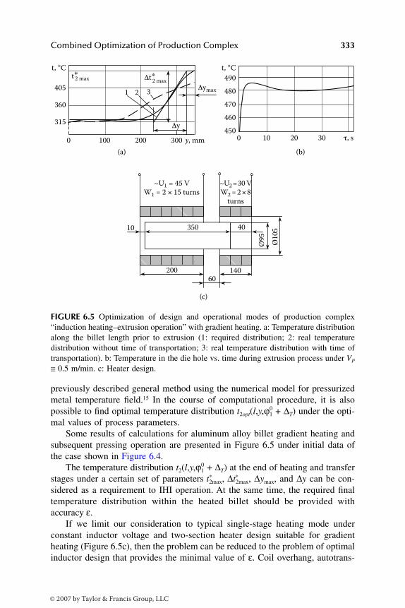
Combined Optimization of Production Complex 333
previously described general method using the numerical model for pressurizedmetal temperature field.15 In the course of computational procedure, it is alsopossible to find optimal temperature distribution t2opt(l,y,ϕ1
0 + ∆T) under the opti-mal values of process parameters.
Some results of calculations for aluminum alloy billet gradient heating andsubsequent pressing operation are presented in Figure 6.5 under initial data ofthe case shown in Figure 6.4.
The temperature distribution t2(l,y,ϕ10 + ∆T) at the end of heating and transfer
stages under a certain set of parameters *t2max, *∆t2max, ∆ymax, and ∆y can be con-sidered as a requirement to IHI operation. At the same time, the required finaltemperature distribution within the heated billet should be provided withaccuracy ε.
If we limit our consideration to typical single-stage heating mode underconstant inductor voltage and two-section heater design suitable for gradientheating (Figure 6.5c), then the problem can be reduced to the problem of optimalinductor design that provides the minimal value of ε. Coil overhang, autotrans-
FIGURE 6.5 Optimization of design and operational modes of production complex“induction heating–extrusion operation” with gradient heating. a: Temperature distributionalong the billet length prior to extrusion (1: required distribution; 2: real temperaturedistribution without time of transportation; 3: real temperature distribution with time oftransportation). b: Temperature in the die hole vs. time during extrusion process under VP
≅ 0.5 m/min. c: Heater design.
(a) (b)
(c)
0
1 2 3
t, °C t, °Ct∗2 max Δt∗
2 max
Δymax
Δy
100 200 300 y, mm
315
360
405
0 10 20 30 τ, s450
460
470
480
490
10 350 40
Ø9
5
Ø1
05
200 140
~U1 = 45 V
W1 = 2 × 15 turns
~U2 = 30 V
W2 = 2 × 8
turns
60
DK6039_C006.fm Page 333 Thursday, June 8, 2006 3:14 PM
© 2007 by Taylor & Francis Group, LLC
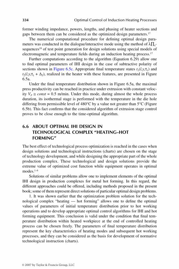
334 Optimal Control of Induction Heating Processes
former winding impedance, powers, lengths, and phasing of heater sections andgaps between them can be considered as the optimized design parameters.17
The numerical computational procedure for defining optimal design para-meters was conducted in the dialogue/interactive mode using the method of λ∏τ-sequences18 of test point generation for design solutions using special models ofelectromagnetic and temperature fields during an induction heating process.17
Further computations according to the algorithm (Equation 6.29) allow oneto find optimal parameters of IHI design in the case of subtractive polarity ofsections shown in Figure 6.5c. Appropriate final temperature states t1(l,y,τ1) andt2(l,y,τ1 + ∆T), realized in the heater with these features, are presented in Figure6.5a.
Under the final temperature distribution shown in Figure 6.5a, the maximalpress productivity can be reached in practice under extrusion with constant veloc-ity VP ≅ const = 0.5 m/min. Under this mode, during almost the whole processduration, its isothermal stage is performed with the temperature in the die holediffering from permissible level of 480°C by a value not greater than 5°C (Figure6.5b). This fact confirms that the considered algorithm of extrusion stage controlproves to be close enough to the time-optimal algorithm.
6.6 ABOUT OPTIMAL IHI DESIGN IN TECHNOLOGICAL COMPLEX “HEATING–HOT FORMING”
The best effect of technological process optimization is reached in the cases whendesign solutions and technological instructions (charts) are chosen on the stageof technology development, and while designing the appropriate part of the wholeproduction complex. These technological and design solutions provide theextreme value of optimized cost function while equipment operates in optimalmodes.1–6
Solutions of similar problems allow one to implement elements of the optimalIHI design in production complexes for metal hot forming. In this regard, thedifferent approaches could be offered, including methods proposed in the presentbook; some of them represent direct solutions of particular optimal design problems.
1. It was shown earlier that the optimization problem solution for the tech-nological complex “heating — hot forming” allows one to define the optimalvalues of parameters of initial temperature distribution prior to hot workingoperations and to develop appropriate optimal control algorithms for IHI and hotforming equipment. This conclusion is valid under the condition that final tem-perature distribution within heated workpiece at the end of controlled heatingprocess can be chosen freely. The parameters of final temperature distributionrepresent the key characteristics of heating modes and subsequent hot workingprocesses, and they can be considered as the basis for development of normativetechnological instruction (charts).
DK6039_C006.fm Page 334 Thursday, June 8, 2006 3:14 PM
© 2007 by Taylor & Francis Group, LLC

Combined Optimization of Production Complex 335
The general method, examples of statement and solution of similar problemfor maximum productivity of the complex “IHI–hot forming equipment” arediscussed in Sections 6.3 through 6.5 under the condition that the permissibleregion for temperature distributions at the end of heating is presented in para-metric form.
2. The solution of the combined optimization problem for processes of heatingand subsequent hot forming could lead to the optimal design solutions for theproduction complex. The proper choice of operating characteristics of heatinginstallations and hot working equipment would provide extreme values of overallcost function for the whole technological line.
In particular, when optimizing the billet output cycle time ϕc in the system“IHI — hot forming equipment,” the complex productivity could be increased,according to the algorithm in Equation (6.21) in the case shown in Figure 6.1cand Figure 6.4, due to the increase of heating installation power and due to thelarger number B1 of simultaneously heated billets (see dotted lines, displacingpoint D2 or D2′).
The same problem could be solved in the case when the condition *θ2min >θ2c
* is true, which means that the stronger press instrument allows less value ofminimum admissible temperature θ2min
* with regard to constraint in Equation(6.19) (see Figure 6.1 through Figure 6.4).
Another way of optimal IHI design respective to the best approximation torequired initial temperature distribution before hot forming is described in Section6.5. An example of the maximum productivity problem solution for the complex“IHI — hot forming equipment” with preliminary gradient billet heating beforepressing is also provided in this section.
3. Definition of spatial-distributed control inputs and optimal inductor lengthin the problem of continuous heating mode optimization (Chapter 5) give answersto the main questions of continuous heater optimal design.
4. Based on the results of the solution of induction heating optimizationproblem, the surfaces in the space of IHI design parameters could be built. Withinthe limits of these surfaces the fixed values of considered cost function I remainconstant (equiscalar surfaces of quality I = const). The set of these surfaces, builtfor different values I = const, allows to define in this space the regions of attainablequality according to chosen performance indexes. The further choice of particularparameter values within specified regions leads to partial realization of the optimalIHI design solutions.
As an example, equiscalar curves ϕ1min0 = const are shown in Figure 6.6 for
ε = , ε = and ε0 = = const, i = 1,2. These curves have been builtusing the solution of several time-optimal problems (see Section 3.1 throughSection 3.4, and Section 3.6) with respect to the basic model (Equation (1.27)through Equation (1.35)) in the plane of dimensionless parameters ξ and Bi underθ0 = const [6].
Each point on these curves corresponds to the computed value of minimumheating process time ϕmin
0 (ξ′, Bi′) or to maximum heating accuracy (ξ′, Bi′)
εmin( )1 εmin
( )2 εmin( )i
εmin( )i
DK6039_C006.fm Page 335 Thursday, June 8, 2006 3:14 PM
© 2007 by Taylor & Francis Group, LLC

336 Optimal Control of Induction Heating Processes
for corresponding to these point values ξ = ξ′ and Bi = Bi′ under chosen valueθ0 = const.
The set of these equiscalar curves allows to find admissible (according togiven cost function, i.e., with respect to process time ϕ1
0 and heating accuracy ε)intervals of parameters ξ and Bi variation. These intervals determine possibleranges of values that define the basic characteristics of IHI design solutions, forexample, possible ranges of supplying current frequency (possible variations ofξ) and parameters of inductor thermal insulation (possible values of Bi) for IHIwith given maximum heating power (under θ0 = const).
FIGURE 6.6 Results of time-optimal heating process under single-stage (a) and two-stage(b) control (θ0 = –1, Γ = 1; θ* = 0; Umax = 1).
(a)
0
2
4
6
8
ξ
0.1
ϕ°1min
= 0.55
0.2 0.3 0.4 0.5 Bi
0.1
0.13
0.6 0.7
0.09
ε(1) = 0.05min
ξ
(b)
0.1 0.2 0.3 0.4 Bi 0
2
4
6
8
0.7
0.75
0.68
0.015 0.026
0.021 0.03 ε(2) =
0.0075min
ϕ°1min
= 0.67
DK6039_C006.fm Page 336 Thursday, June 8, 2006 3:14 PM
© 2007 by Taylor & Francis Group, LLC
Combined Optimization of Production Complex 337
Building of corresponding equiscalar surfaces in the space of parameters ξ,Bi, θ0 and their sections for ξ = const and Bi = const allows one to include thepower of heating installation (the value θ0) into the set of design parameters.
5. If we supplement unknown parameters ∆i, i = of sought optimal controlalgorithms (see Section 3.7) by parameters ∆i, i = ,
characterizing IHI
design solutions, then the set of all these values ∆i, i = could be found as aresult of the combined optimization problem solution for optimal IHI control anddesign with regard to chosen cost criteria.
A representative example was presented earlier in Section 4.5.3, where thebillet overhang in static induction installation can be considered as additionalsought-for parameter.
A similar problem of combined optimization could be reduced to the state-ment of mathematical programming problem of the type in Equation (3.38), butit should be solved with respect to “extended” vector ∆ = (∆i), i = . In thiscase, the main feature consists in the fact that for typical economic criteria ofcombined optimization (in contrast to local criteria for optimal control problems),the global minimum of overall cost function is reached, as a rule, on the optimaldesign solution. Consequently, equality of the type in Equation (3.42) becomestrue on the set of values ∆i, i = . As was shown in Section 3.7, thisequality violates assumptions, for which main properties of final temperaturedistribution within heated billet (see Equation (3.39) and Equation (3.40)) remainvalid.
In that case it is not possible to use method proposed in the present text forparametric optimization of induction heating processes, because it is based onthese properties. To find the solution of considered problem, it is necessary toapply the additional procedure of searching (by known methods) for extremevalue of overall cost function within the set of optimized design solutions. Thisprocedure should provide (as an intermediate step) computation of optimal controlalgorithms according to the general techniques of Chapter 3 through Chapter 5on all tested elements of the design solutions set.
Let us illustrate the obtained conclusions by the example, when the powerPu of the heating installation presents the single sought parameter of the designsolution. Let us also consider only the typical situation, when maximum IHIthroughput corresponds to maximum of obtained economical profit. Then thetotal cost of the heating process implementation can be accepted as the overallcost function for optimal IHI design and control. The total cost is proportionalto the duration of the heating stage and capital expenditures (proportional to Pu
2):
. (6.44)
1, NN N+1 1,
1 1, N
1 1, N
N N+1 1,
I k P k Pu uPu
= ( ) + →1 1 22τ min min
DK6039_C006.fm Page 337 Thursday, June 8, 2006 3:14 PM
© 2007 by Taylor & Francis Group, LLC

338 Optimal Control of Induction Heating Processes
Here τ1min is the minimum time required for the heating process, that is definedby parameter vector ∆0 of time-optimal control inputs (for instance, in the formof sum in Equation (2.31)).
The problem is reduced to searching for optimal heating power Pu opt andparameters ∆0 providing minimum value of criterion in Equation (6.44) undergiven cost factors K1 and K2.
For each fixed value Pu, the corresponding “own” solution ∆0 (Pu) of properlyset time-optimal problem exists. This solution is found using methods describedearlier in Chapter 3 through Chapter 5.
The subsequent solutions for different values of Pu allows us to find monot-onously decreasing dependency τ1min(Pu). When increasing the second componentin Equation (6.44), the cost function in Equation (6.44) reaches its global mini-mum at the point Pu =Pu opt (Figure 6.7) which is defined by correlation
. (6.45)
The special case takes place when given cost criteria have no extreme pointson the set of considered design solutions. Under existing real-life constraints, theminimum of cost function is always reached at one of boundaries of possibledesign parameters range.
This information usually allows us to find optimal values of design para-meters, and then it remains only to solve the optimal control problem withoutconsidering “extended” set of sought-for unknowns.
Such a situation appears, in particular, when searching for optimal values ofsupplying current frequency (parameter ξ) and Bi criterion (defining the qualityof inductor thermal refractory) in the time-optimal problem with heating power
FIGURE 6.7 Value of economic cost I criterion as a function of heat power.
P k P k Pu optP
u uu
= ( ) +
arg min min1 1 22τ
I
Pu opt
k2Pu2
k1τ°1min
Pu
DK6039_C006.fm Page 338 Thursday, June 8, 2006 3:14 PM
© 2007 by Taylor & Francis Group, LLC
Combined Optimization of Production Complex 339
control. Optimal values of parameter ξ and Bi criterion comply often with theirminimal admissible values.
REFERENCES
1. Butkovskij, A.G., Malyj, S.A., and Andreev, Yu.N., Optimal Control of MetalsHeating, Metallurgy, Moscow, 1972.
2. Butkovskij, A.G., Malyj, S.A., and Andreev, Yu.N., Control of Metals Heating,Metallurgy, Moscow, 1981.
3. Malyj, S.A., Energy Conserving Heating of Metals, Metallurgy, Moscow, 1967.4. Andreev, Yu.N., Optimal Design of Heating Installations, Mashinostroenie, Mos-
cow, 1983.5. Rapoport, E.Ya., Optimization of heating and extrusion modes in technological
complex “heater–press,” Physica i himija obrabotki materialov, 3, 66, 1985.6. Rapoport, E.Ya., Optimization of Induction Heating of Metals, Metallurgy, Mos-
cow, 1993.7. Perlin, I.L. and Gajtbarg, L.H., Theory of Metals Extrusion, Metallurgy, Moscow,
1975.8. Gun, G.Ya., Poluhin, P.I., and Ganelin, D.Yu., Mathematical modeling of axially
symmetrical steady-state processes of metals extrusion, Izvestija vuzov, Chernajametallurgija, 5, 82, 1976.
9. Gun, G.Ya., Basics of Metals Treatment by Pressure, Metallurgy, Moscow, 1980.10. Gun, G.Ya. et al., Extrusion of Aluminum Alloys (Mathematical Modeling and
Optimization), Metallurgy, Moscow, 1974.11. Scholobov, V.V. and Zverev, G.I., Metals Extrusion, Metallurgy, Moscow, 1971.12. Khenzel, A.A., Optimization of Energy Consumption in Extrusion Processes,
Metallurgy, Moscow, 1985.13. Rapoport, E.Ya., Mathematical modelling of metals temperature fields during
extrusion process, Physica i Khimija obrabotki materialov, Moscow, 1, 29, 1980.14. Gun, G.Ya. et al., Plastic Deformation of Metals, Metallurgy, Moscow, 196815. Zimin, L.S., Rapoport, E.Ya., and Kondrashov, S.V., Determining temperature
field of aluminum alloy cylindrical billet during axially symmetrical extrusion,Algoritmy i programmy, 1. 64, 1986.
16. Rapoport, E.Ya., Theory and algorithms optimal control of metals induction heat-ing prior to pressure processing, D.D. thesis, Institut stali i splavov, Moscow, 1983.
17. Zimin L.S. et al., Reducing energy usage efficiency in Volga region, Saratov StateUniversity, Saratov, 122, 1990.
18. Sobol, I.M. and Statnikov, R.B., Selection of Optimal Parameters in Multi-CriteriaProblems, Nauka, Moscow, 1981.
DK6039_C006.fm Page 339 Thursday, June 8, 2006 3:14 PM
© 2007 by Taylor & Francis Group, LLC
341
Conclusion
The main goal of this book is to provide a detailed systematic description of basictheory and practical applications of new methods for solving engineering opti-mization problems. The authors show the advantages of new, highly-effectiveapproaches for the optimization of induction heating processes prior to metalworking. These new optimization approaches deliver a essential advantages overthe presently used classical approaches. Novel optimization techniques can beapplied not only to induction heating applications but also to the optimization ofa much wider range of technological processes.
The described technique proves to be efficient not only for a wide range ofIHP optimization problems and a large variety of specific mathematical models,but for various cost functions, control input types, special requirements, andrestraints of practical technology as well.
The method is based on the fundamental properties of temperature distribu-tions of induction heating processes, which were ascertained and described hereby authors; these properties remain constant for all of the stated problems.
In a particular application, the use of these properties allows the developmentof an appropriate set of equations to sought-for parameters of the optimal processtaking into consideration specifics of the particular physical properties of thetechnological process.
The authors hope that readers will be able to apply the described optimizationtechnique to similar problems and for the problems that remain beyond the boundsof this monograph.
Rigorous proof of the alternance method is not given in this book because itrequires the authors to be fluent in advanced mathematics and have specialknowledge in the area that is usually far beyond area of interest of majority ofusers of induction heating technology. We would suggest to those who are inter-ested in the rigorous study of a particular topic discussed in this book to see thelistings given in the reference sections of each chapter.
The authors will deeply appreciate the readers’ comments regarding novel,alternate optimization techniques that were described here in the application ofthe optimization of induction metal heating processes.
DK6039_C007.fm Page 341 Thursday, May 25, 2006 12:06 PM
© 2007 by Taylor & Francis Group, LLC