Embed Size (px)
Citation preview
Optimal Control & Viscosity SolutionsTutorial Slides from
Banff International Research Station Workshop 11w5086:Advancing Numerical Methods for
Viscosity Solutions and Applications
Ian M. [email protected]
http://www.cs.ubc.ca/˜mitchell
University of British ColumbiaDepartment of Computer Science
February 2011

Outline
∙ Optimal control: models of system dynamics and objective functionals
∙ The value function and the dynamic programming principle
∙ A formal derivation of the Hamilton-Jacobi(-Bellman) equation
∙ Viscosity solutions and a rigorous derivation
∙ Other types of Hamilton-Jacobi equations in control
∙ Optimal control problems with analytic solutions
∙ References
Optimal Control & Viscosity Solutions Ian M. Mitchell— UBC Computer Science 2/ 41
Control Theory
∙ Control theory is the mathematical study of methods to steer the evolution ofa dynamic system to achieve desired goals
∙ For example, stability or tracking a reference
∙ Optimal control is a branch of control theory that seeks to steer the evolutionso as to optimize a specific objective functional
∙ There are close connections with calculus of variations
∙ Mathematical study of control requires predictive models of the systemevolution
∙ Assume Markovian models: everything relevant to future evolution of thesystem is captured in the current state
∙ Many classes of models, but we will talk primarily about deterministic,continuous state, continuous time systems
∙ Other continuous models: stochastic DEs, delay DEs, differential algebraticequations, differential inclusions, . . .
∙ Other classes of dynamic evolution: discrete time (eg: discrete event), discretestate (eg: Markov chains), . . .
Optimal Control & Viscosity Solutions Ian M. Mitchell— UBC Computer Science 3/ 41
System Models
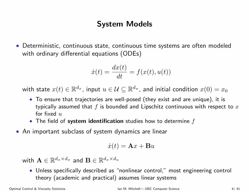
∙ Deterministic, continuous state, continuous time systems are often modeledwith ordinary differential equations (ODEs)
x(t) =dx(t)
dt= f(x(t), u(t))
with state x(t) ∈ ℝdx , input u ∈ U ⊆ ℝdu , and initial condition x(0) = x0
∙ To ensure that trajectories are well-posed (they exist and are unique), it istypically assumed that f is bounded and Lipschitz continuous with respect to xfor fixed u
∙ The field of system identification studies how to determine f
∙ An important subclass of system dynamics are linear
x(t) = Ax+ Bu
with A ∈ ℝdx×dx and B ∈ ℝdx×du
∙ Unless specifically described as “nonlinear control,” most engineering controltheory (academic and practical) assumes linear systems
Optimal Control & Viscosity Solutions Ian M. Mitchell— UBC Computer Science 4/ 41
Optimal Control Objectives
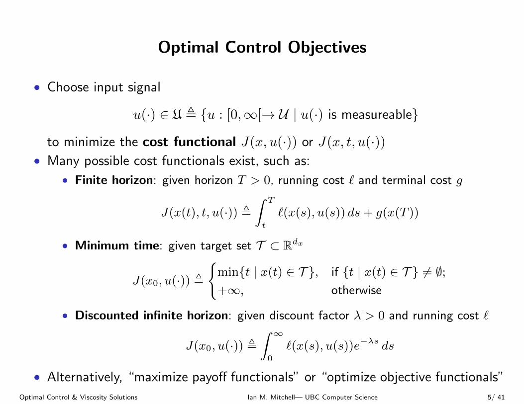
∙ Choose input signal
u(⋅) ∈ U ≜ {u : [0,∞[→ U ∣ u(⋅) is measureable}
to minimize the cost functional J(x, u(⋅)) or J(x, t, u(⋅))∙ Many possible cost functionals exist, such as:
∙ Finite horizon: given horizon T > 0, running cost ℓ and terminal cost g
J(x(t), t, u(⋅)) ≜∫ T
t
ℓ(x(s), u(s)) ds+ g(x(T ))
∙ Minimum time: given target set T ⊂ ℝdx
J(x0, u(⋅)) ≜
{min{t ∣ x(t) ∈ T }, if {t ∣ x(t) ∈ T } ∕= ∅;+∞, otherwise
∙ Discounted infinite horizon: given discount factor � > 0 and running cost ℓ
J(x0, u(⋅)) ≜∫ ∞0
ℓ(x(s), u(s))e−�s ds
∙ Alternatively, “maximize payoff functionals” or “optimize objective functionals”
Optimal Control & Viscosity Solutions Ian M. Mitchell— UBC Computer Science 5/ 41

Outline
∙ Optimal control: models of system dynamics and objective functionals
∙ The value function and the dynamic programming principle
∙ A formal derivation of the Hamilton-Jacobi(-Bellman) equation
∙ Viscosity solutions and a rigorous derivation
∙ Other types of Hamilton-Jacobi equations in control
∙ Optimal control problems with analytic solutions
∙ References
Optimal Control & Viscosity Solutions Ian M. Mitchell— UBC Computer Science 6/ 41
Value Functions
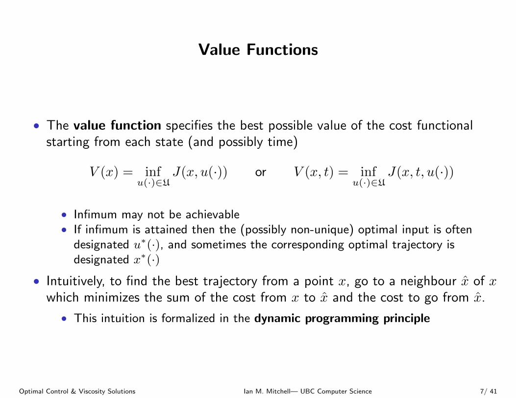
∙ The value function specifies the best possible value of the cost functionalstarting from each state (and possibly time)
V (x) = infu(⋅)∈U
J(x, u(⋅)) or V (x, t) = infu(⋅)∈U
J(x, t, u(⋅))
∙ Infimum may not be achievable∙ If infimum is attained then the (possibly non-unique) optimal input is often
designated u∗(⋅), and sometimes the corresponding optimal trajectory isdesignated x∗(⋅)
∙ Intuitively, to find the best trajectory from a point x, go to a neighbour x of xwhich minimizes the sum of the cost from x to x and the cost to go from x.
∙ This intuition is formalized in the dynamic programming principle
Optimal Control & Viscosity Solutions Ian M. Mitchell— UBC Computer Science 7/ 41
Dynamic Programming Principle
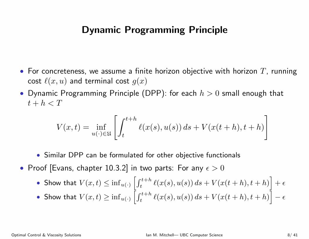
∙ For concreteness, we assume a finite horizon objective with horizon T , runningcost ℓ(x, u) and terminal cost g(x)
∙ Dynamic Programming Principle (DPP): for each ℎ > 0 small enough thatt+ ℎ < T
V (x, t) = infu(⋅)∈U
[∫ t+ℎ
t
ℓ(x(s), u(s)) ds+ V (x(t+ ℎ), t+ ℎ)
]
∙ Similar DPP can be formulated for other objective functionals
∙ Proof [Evans, chapter 10.3.2] in two parts: For any � > 0
∙ Show that V (x, t) ≤ infu(⋅)
[∫ t+ℎt
ℓ(x(s), u(s)) ds+ V (x(t+ ℎ), t+ ℎ)]
+ �
∙ Show that V (x, t) ≥ infu(⋅)
[∫ t+ℎt
ℓ(x(s), u(s)) ds+ V (x(t+ ℎ), t+ ℎ)]− �
Optimal Control & Viscosity Solutions Ian M. Mitchell— UBC Computer Science 8/ 41
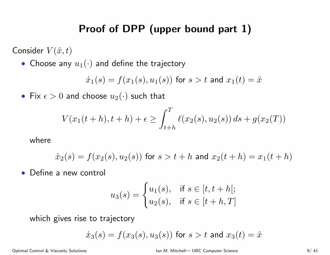
Proof of DPP (upper bound part 1)
Consider V (x, t)
∙ Choose any u1(⋅) and define the trajectory
x1(s) = f(x1(s), u1(s)) for s > t and x1(t) = x
∙ Fix � > 0 and choose u2(⋅) such that
V (x1(t+ ℎ), t+ ℎ) + � ≥∫ T
t+ℎ
ℓ(x2(s), u2(s)) ds+ g(x2(T ))
where
x2(s) = f(x2(s), u2(s)) for s > t+ ℎ and x2(t+ ℎ) = x1(t+ ℎ)
∙ Define a new control
u3(s) =
{u1(s), if s ∈ [t, t+ ℎ[;
u2(s), if s ∈ [t+ ℎ, T ]
which gives rise to trajectory
x3(s) = f(x3(s), u3(s)) for s > t and x3(t) = x
Optimal Control & Viscosity Solutions Ian M. Mitchell— UBC Computer Science 9/ 41
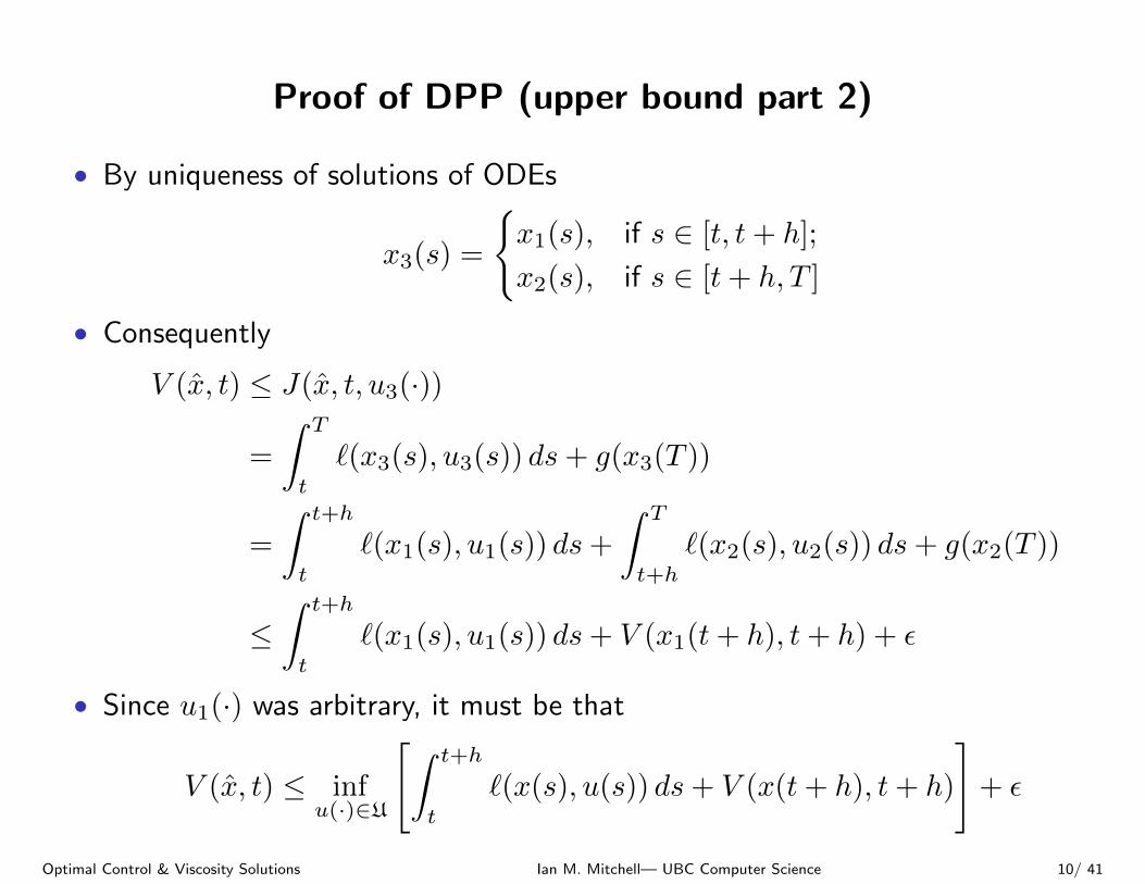
Proof of DPP (upper bound part 2)
∙ By uniqueness of solutions of ODEs
x3(s) =
{x1(s), if s ∈ [t, t+ ℎ];
x2(s), if s ∈ [t+ ℎ, T ]
∙ Consequently
V (x, t) ≤ J(x, t, u3(⋅))
=
∫ T
t
ℓ(x3(s), u3(s)) ds+ g(x3(T ))
=
∫ t+ℎ
t
ℓ(x1(s), u1(s)) ds+
∫ T
t+ℎ
ℓ(x2(s), u2(s)) ds+ g(x2(T ))
≤∫ t+ℎ
t
ℓ(x1(s), u1(s)) ds+ V (x1(t+ ℎ), t+ ℎ) + �
∙ Since u1(⋅) was arbitrary, it must be that
V (x, t) ≤ infu(⋅)∈U
[∫ t+ℎ
t
ℓ(x(s), u(s)) ds+ V (x(t+ ℎ), t+ ℎ)
]+ �
Optimal Control & Viscosity Solutions Ian M. Mitchell— UBC Computer Science 10/ 41
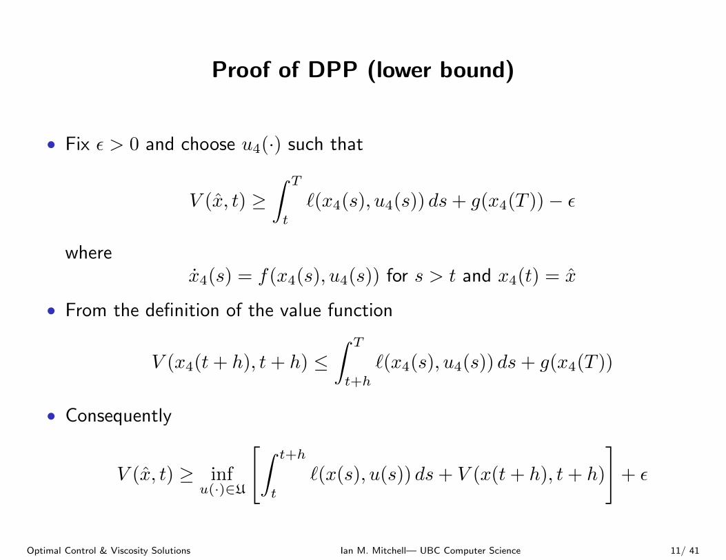
Proof of DPP (lower bound)
∙ Fix � > 0 and choose u4(⋅) such that
V (x, t) ≥∫ T
t
ℓ(x4(s), u4(s)) ds+ g(x4(T ))− �
wherex4(s) = f(x4(s), u4(s)) for s > t and x4(t) = x
∙ From the definition of the value function
V (x4(t+ ℎ), t+ ℎ) ≤∫ T
t+ℎ
ℓ(x4(s), u4(s)) ds+ g(x4(T ))
∙ Consequently
V (x, t) ≥ infu(⋅)∈U
[∫ t+ℎ
t
ℓ(x(s), u(s)) ds+ V (x(t+ ℎ), t+ ℎ)
]+ �
Optimal Control & Viscosity Solutions Ian M. Mitchell— UBC Computer Science 11/ 41
Outline
∙ Optimal control: models of system dynamics and objective functionals
∙ The value function and the dynamic programming principle
∙ A formal derivation of the Hamilton-Jacobi(-Bellman) equation
∙ Viscosity solutions and a rigorous derivation
∙ Other types of Hamilton-Jacobi equations in control
∙ Optimal control problems with analytic solutions
∙ References
Optimal Control & Viscosity Solutions Ian M. Mitchell— UBC Computer Science 12/ 41
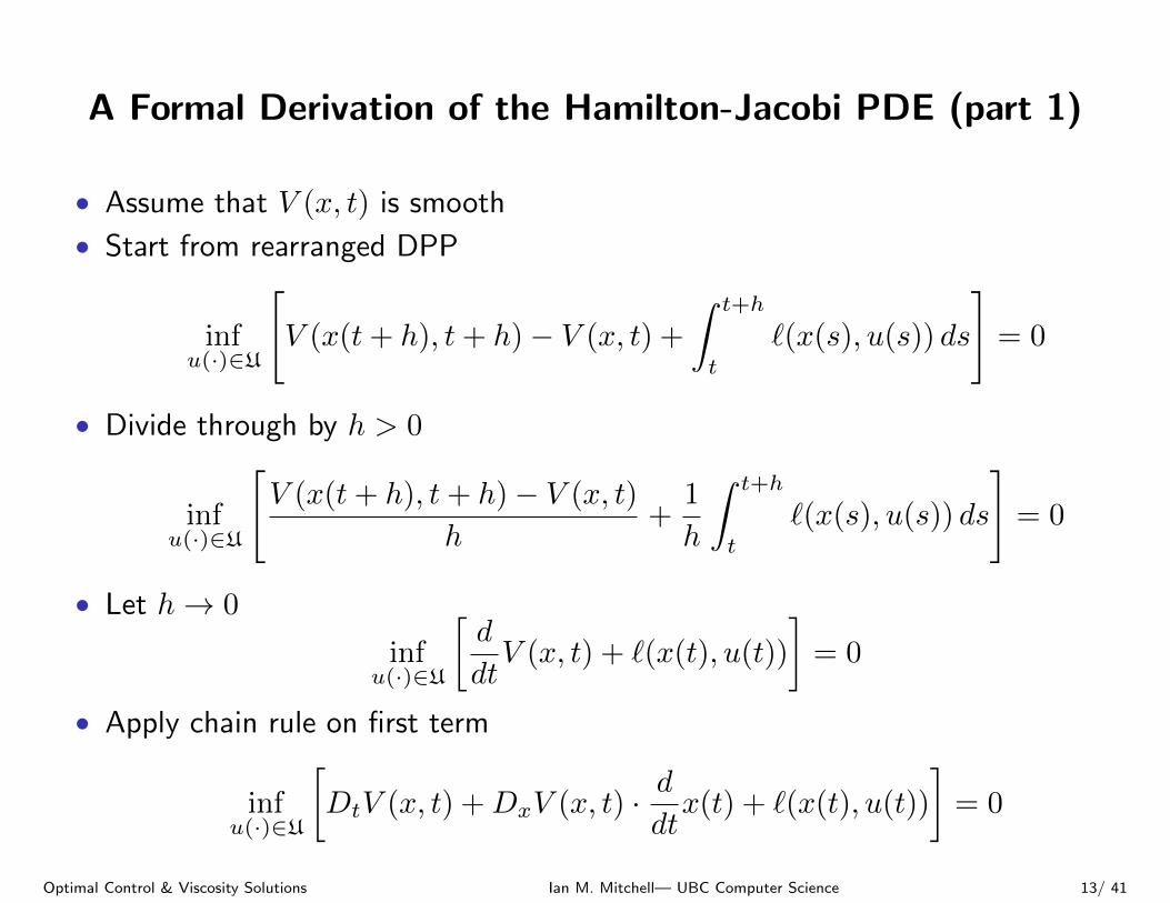
A Formal Derivation of the Hamilton-Jacobi PDE (part 1)
∙ Assume that V (x, t) is smooth
∙ Start from rearranged DPP
infu(⋅)∈U
[V (x(t+ ℎ), t+ ℎ)− V (x, t) +
∫ t+ℎ
t
ℓ(x(s), u(s)) ds
]= 0
∙ Divide through by ℎ > 0
infu(⋅)∈U
[V (x(t+ ℎ), t+ ℎ)− V (x, t)
ℎ+
1
ℎ
∫ t+ℎ
t
ℓ(x(s), u(s)) ds
]= 0
∙ Let ℎ→ 0
infu(⋅)∈U
[d
dtV (x, t) + ℓ(x(t), u(t))
]= 0
∙ Apply chain rule on first term
infu(⋅)∈U
[DtV (x, t) +DxV (x, t) ⋅ d
dtx(t) + ℓ(x(t), u(t))
]= 0
Optimal Control & Viscosity Solutions Ian M. Mitchell— UBC Computer Science 13/ 41
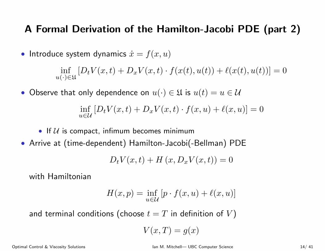
A Formal Derivation of the Hamilton-Jacobi PDE (part 2)
∙ Introduce system dynamics x = f(x, u)
infu(⋅)∈U
[DtV (x, t) +DxV (x, t) ⋅ f(x(t), u(t)) + ℓ(x(t), u(t))] = 0
∙ Observe that only dependence on u(⋅) ∈ U is u(t) = u ∈ U
infu∈U
[DtV (x, t) +DxV (x, t) ⋅ f(x, u) + ℓ(x, u)] = 0
∙ If U is compact, infimum becomes minimum
∙ Arrive at (time-dependent) Hamilton-Jacobi(-Bellman) PDE
DtV (x, t) +H (x,DxV (x, t)) = 0
with Hamiltonian
H(x, p) = infu∈U
[p ⋅ f(x, u) + ℓ(x, u)]
and terminal conditions (choose t = T in definition of V )
V (x, T ) = g(x)
Optimal Control & Viscosity Solutions Ian M. Mitchell— UBC Computer Science 14/ 41
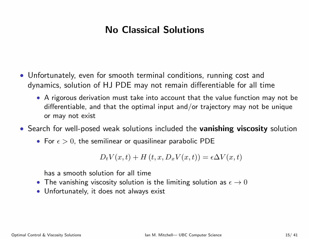
No Classical Solutions
∙ Unfortunately, even for smooth terminal conditions, running cost anddynamics, solution of HJ PDE may not remain differentiable for all time
∙ A rigorous derivation must take into account that the value function may not bedifferentiable, and that the optimal input and/or trajectory may not be uniqueor may not exist
∙ Search for well-posed weak solutions included the vanishing viscosity solution
∙ For � > 0, the semilinear or quasilinear parabolic PDE
DtV (x, t) +H (t, x,DxV (x, t)) = �ΔV (x, t)
has a smooth solution for all time∙ The vanishing viscosity solution is the limiting solution as �→ 0∙ Unfortunately, it does not always exist
Optimal Control & Viscosity Solutions Ian M. Mitchell— UBC Computer Science 15/ 41

Outline
∙ Optimal control: models of system dynamics and objective functionals
∙ The value function and the dynamic programming principle
∙ A formal derivation of the Hamilton-Jacobi(-Bellman) equation
∙ Viscosity solutions and a rigorous derivation
∙ Other types of Hamilton-Jacobi equations in control
∙ Optimal control problems with analytic solutions
∙ References
Optimal Control & Viscosity Solutions Ian M. Mitchell— UBC Computer Science 16/ 41
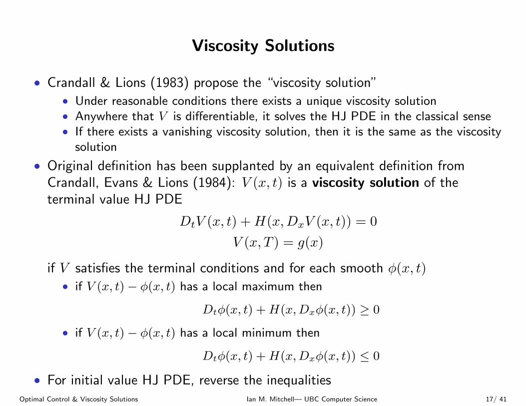
Viscosity Solutions
∙ Crandall & Lions (1983) propose the “viscosity solution”∙ Under reasonable conditions there exists a unique viscosity solution∙ Anywhere that V is differentiable, it solves the HJ PDE in the classical sense∙ If there exists a vanishing viscosity solution, then it is the same as the viscosity
solution
∙ Original definition has been supplanted by an equivalent definition fromCrandall, Evans & Lions (1984): V (x, t) is a viscosity solution of theterminal value HJ PDE
DtV (x, t) +H(x,DxV (x, t)) = 0
V (x, T ) = g(x)
if V satisfies the terminal conditions and for each smooth �(x, t)∙ if V (x, t)− �(x, t) has a local maximum then
Dt�(x, t) +H(x,Dx�(x, t)) ≥ 0
∙ if V (x, t)− �(x, t) has a local minimum then
Dt�(x, t) +H(x,Dx�(x, t)) ≤ 0
∙ For initial value HJ PDE, reverse the inequalitiesOptimal Control & Viscosity Solutions Ian M. Mitchell— UBC Computer Science 17/ 41
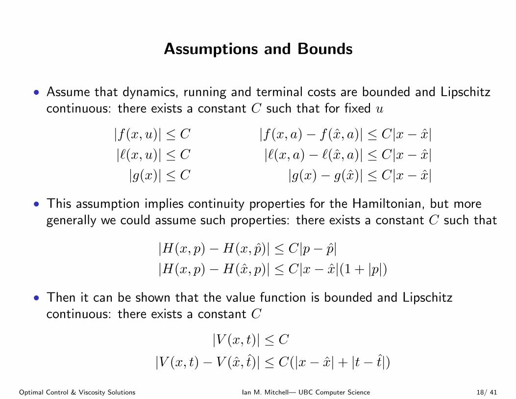
Assumptions and Bounds
∙ Assume that dynamics, running and terminal costs are bounded and Lipschitzcontinuous: there exists a constant C such that for fixed u
∣f(x, u)∣ ≤ C ∣f(x, a)− f(x, a)∣ ≤ C∣x− x∣∣ℓ(x, u)∣ ≤ C ∣ℓ(x, a)− ℓ(x, a)∣ ≤ C∣x− x∣∣g(x)∣ ≤ C ∣g(x)− g(x)∣ ≤ C∣x− x∣
∙ This assumption implies continuity properties for the Hamiltonian, but moregenerally we could assume such properties: there exists a constant C such that
∣H(x, p)−H(x, p)∣ ≤ C∣p− p∣∣H(x, p)−H(x, p)∣ ≤ C∣x− x∣(1 + ∣p∣)
∙ Then it can be shown that the value function is bounded and Lipschitzcontinuous: there exists a constant C
∣V (x, t)∣ ≤ C∣V (x, t)− V (x, t)∣ ≤ C(∣x− x∣+ ∣t− t∣)
Optimal Control & Viscosity Solutions Ian M. Mitchell— UBC Computer Science 18/ 41
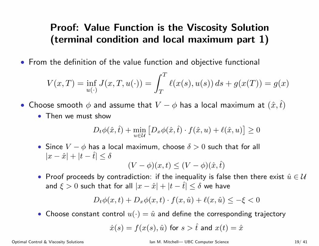
Proof: Value Function is the Viscosity Solution(terminal condition and local maximum part 1)
∙ From the definition of the value function and objective functional
V (x, T ) = infu(⋅)
J(x, T, u(⋅)) =
∫ T
T
ℓ(x(s), u(s)) ds+ g(x(T )) = g(x)
∙ Choose smooth � and assume that V − � has a local maximum at (x, t)∙ Then we must show
Dt�(x, t) + minu∈U
[Dx�(x, t) ⋅ f(x, u) + ℓ(x, u)
]≥ 0
∙ Since V − � has a local maximum, choose � > 0 such that for all∣x− x∣+ ∣t− t∣ ≤ �
(V − �)(x, t) ≤ (V − �)(x, t)
∙ Proof proceeds by contradiction: if the inequality is false then there exist u ∈ Uand � > 0 such that for all ∣x− x∣+ ∣t− t∣ ≤ � we have
Dt�(x, t) +Dx�(x, t) ⋅ f(x, u) + ℓ(x, u) ≤ −� < 0
∙ Choose constant control u(⋅) = u and define the corresponding trajectory
x(s) = f(x(s), u) for s > t and x(t) = x
Optimal Control & Viscosity Solutions Ian M. Mitchell— UBC Computer Science 19/ 41

Proof: Value Function is the Viscosity Solution(local maximum part 2)
∙ Working on contradiction if V − � has a local maximum at (x, t)∙ Choose ℎ ∈ [0, �] small enough that ∣x(s)− x∣ ≤ � for s ∈ [t, t+ ℎ] so that
Dt�(x(s), s) +Dx�(x(s), s) ⋅ f(x(s), u) + ℓ(x(s), u) ≤ −�
∙ Because V − � has a local maximum
V (x(t+ ℎ), t+ ℎ)− V (x, t) ≤ �(x(t+ ℎ), t+ ℎ)− �(x, t)
=
∫ t+ℎ
t
d
ds�(x(s), s) ds
=
∫ t+ℎ
t
Dt�(x(s), s) +Dx�(x(s), s) ⋅ f(x(s), u) ds
∙ From the DPP
V (x, t) ≤∫ t+ℎ
t
ℓ(x(s), u) ds+ V (x(t+ ℎ), t+ ℎ)
∙ Therefore we arrive at the contradiction
0 ≤∫ t+ℎ
t
Dt�(x(s), s) +Dx�(x(s), s) ⋅ f(x(s), u) + ℓ(x(s), u) ds ≤ −�ℎ
Optimal Control & Viscosity Solutions Ian M. Mitchell— UBC Computer Science 20/ 41
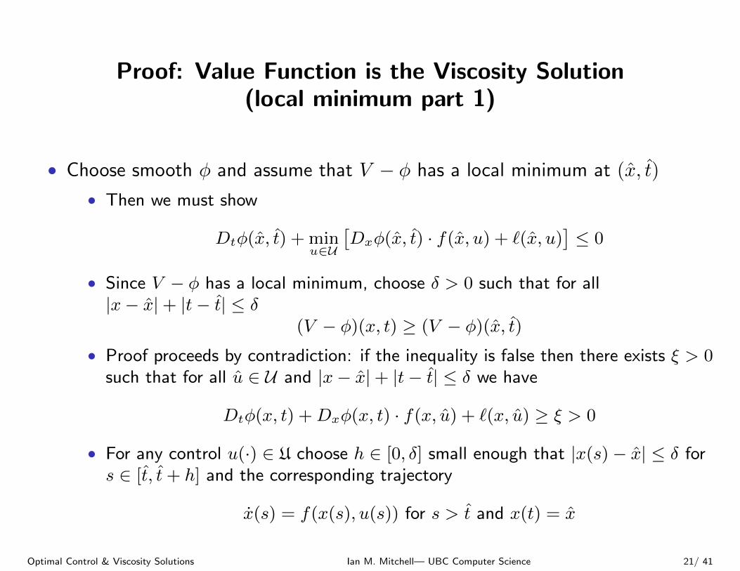
Proof: Value Function is the Viscosity Solution(local minimum part 1)
∙ Choose smooth � and assume that V − � has a local minimum at (x, t)
∙ Then we must show
Dt�(x, t) + minu∈U
[Dx�(x, t) ⋅ f(x, u) + ℓ(x, u)
]≤ 0
∙ Since V − � has a local minimum, choose � > 0 such that for all∣x− x∣+ ∣t− t∣ ≤ �
(V − �)(x, t) ≥ (V − �)(x, t)
∙ Proof proceeds by contradiction: if the inequality is false then there exists � > 0such that for all u ∈ U and ∣x− x∣+ ∣t− t∣ ≤ � we have
Dt�(x, t) +Dx�(x, t) ⋅ f(x, u) + ℓ(x, u) ≥ � > 0
∙ For any control u(⋅) ∈ U choose ℎ ∈ [0, �] small enough that ∣x(s)− x∣ ≤ � fors ∈ [t, t+ ℎ] and the corresponding trajectory
x(s) = f(x(s), u(s)) for s > t and x(t) = x
Optimal Control & Viscosity Solutions Ian M. Mitchell— UBC Computer Science 21/ 41
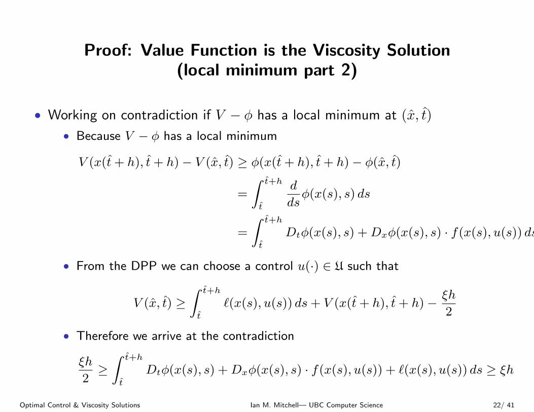
Proof: Value Function is the Viscosity Solution(local minimum part 2)
∙ Working on contradiction if V − � has a local minimum at (x, t)
∙ Because V − � has a local minimum
V (x(t+ ℎ), t+ ℎ)− V (x, t) ≥ �(x(t+ ℎ), t+ ℎ)− �(x, t)
=
∫ t+ℎ
t
d
ds�(x(s), s) ds
=
∫ t+ℎ
t
Dt�(x(s), s) +Dx�(x(s), s) ⋅ f(x(s), u(s)) ds
∙ From the DPP we can choose a control u(⋅) ∈ U such that
V (x, t) ≥∫ t+ℎ
t
ℓ(x(s), u(s)) ds+ V (x(t+ ℎ), t+ ℎ)− �ℎ
2
∙ Therefore we arrive at the contradiction
�ℎ
2≥∫ t+ℎ
t
Dt�(x(s), s) +Dx�(x(s), s) ⋅ f(x(s), u(s)) + ℓ(x(s), u(s)) ds ≥ �ℎ
Optimal Control & Viscosity Solutions Ian M. Mitchell— UBC Computer Science 22/ 41
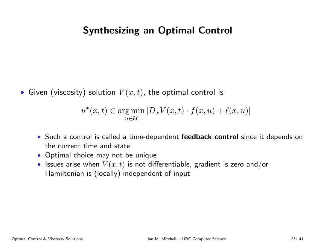
Synthesizing an Optimal Control
∙ Given (viscosity) solution V (x, t), the optimal control is
u∗(x, t) ∈ arg minu∈U
[DxV (x, t) ⋅ f(x, u) + ℓ(x, u)]
∙ Such a control is called a time-dependent feedback control since it depends onthe current time and state
∙ Optimal choice may not be unique∙ Issues arise when V (x, t) is not differentiable, gradient is zero and/or
Hamiltonian is (locally) independent of input
Optimal Control & Viscosity Solutions Ian M. Mitchell— UBC Computer Science 23/ 41

Outline
∙ Optimal control: models of system dynamics and objective functionals
∙ The value function and the dynamic programming principle
∙ A formal derivation of the Hamilton-Jacobi(-Bellman) equation
∙ Viscosity solutions and a rigorous derivation
∙ Other types of Hamilton-Jacobi equations in control
∙ Optimal control problems with analytic solutions
∙ References
Optimal Control & Viscosity Solutions Ian M. Mitchell— UBC Computer Science 24/ 41
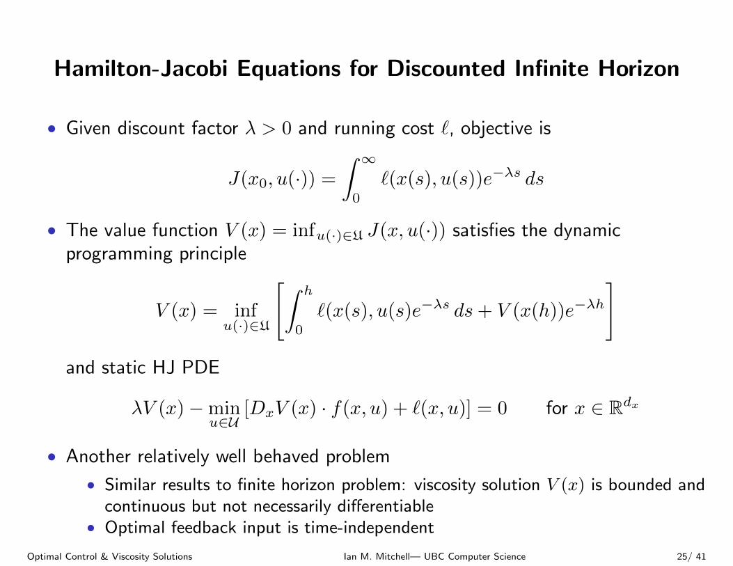
Hamilton-Jacobi Equations for Discounted Infinite Horizon
∙ Given discount factor � > 0 and running cost ℓ, objective is
J(x0, u(⋅)) =
∫ ∞0
ℓ(x(s), u(s))e−�s ds
∙ The value function V (x) = infu(⋅)∈U J(x, u(⋅)) satisfies the dynamicprogramming principle
V (x) = infu(⋅)∈U
[∫ ℎ
0
ℓ(x(s), u(s)e−�s ds+ V (x(ℎ))e−�ℎ
]and static HJ PDE
�V (x)−minu∈U
[DxV (x) ⋅ f(x, u) + ℓ(x, u)] = 0 for x ∈ ℝdx
∙ Another relatively well behaved problem
∙ Similar results to finite horizon problem: viscosity solution V (x) is bounded andcontinuous but not necessarily differentiable
∙ Optimal feedback input is time-independent
Optimal Control & Viscosity Solutions Ian M. Mitchell— UBC Computer Science 25/ 41
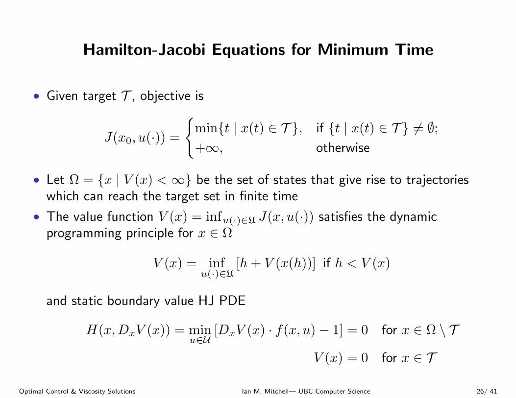
Hamilton-Jacobi Equations for Minimum Time
∙ Given target T , objective is
J(x0, u(⋅)) =
{min{t ∣ x(t) ∈ T }, if {t ∣ x(t) ∈ T } ∕= ∅;+∞, otherwise
∙ Let Ω = {x ∣ V (x) <∞} be the set of states that give rise to trajectorieswhich can reach the target set in finite time
∙ The value function V (x) = infu(⋅)∈U J(x, u(⋅)) satisfies the dynamicprogramming principle for x ∈ Ω
V (x) = infu(⋅)∈U
[ℎ+ V (x(ℎ))] if ℎ < V (x)
and static boundary value HJ PDE
H(x,DxV (x)) = minu∈U
[DxV (x) ⋅ f(x, u)− 1] = 0 for x ∈ Ω ∖ T
V (x) = 0 for x ∈ T
Optimal Control & Viscosity Solutions Ian M. Mitchell— UBC Computer Science 26/ 41
Small Time Local Controllability and the Static HJ PDE
∙ A system is small time locally controllable (STLC) at a state x if the set ofstates which give rise to trajectories which reach x contains x in its interior forall positive times
∙ Intuitively, the system can move in any direction∙ Many important types of system are not STLC
∙ If dynamics are STLC everywhere then the static HJ PDE is relatively wellbehaved: the viscosity solution V (x) is bounded and continuous (but notnecessarily differentiable) and Ω = ℝdx
∙ If dynamics are not STLC then there may not be a bounded continuousviscosity solution which solves the PDE and/or Ω must be determined
Optimal Control & Viscosity Solutions Ian M. Mitchell— UBC Computer Science 27/ 41
Disturbance Parameters
Sometimes the dynamics are influenced by additional parameters
x = f(x, u, v)
where v ∈ ℝdv are not known and are not controllable. There are two typical waysof treating these disturbance inputs
∙ Stochastic: v(t) ∼ V where V is some distribution
∙ Modelled by stochastic differential equations (SDEs) in continuous case, orvarious probabilistic models in discrete settings (Markov chains, discrete statePoisson processes, etc)
∙ Optimal control of SDEs leads to Fokker-Plank or Kolmogorov PDEs: secondorder versions of the HJ PDE
∙ Bounded value: v(t) ∈ V where V ⊆ ℝdv is a specified set
∙ Modelled by standard ODEs with multiple inputs∙ Robust or worst-case treatment of disturbance input is modelled by two player
zero sum games and HJ PDE with nonconvex Hamiltonians
Optimal Control & Viscosity Solutions Ian M. Mitchell— UBC Computer Science 28/ 41
Dynamics, Objective Functional and Player Knowledgein Differential Games
∙ Dynamics and objective functional are almost the same as in the single inputcase; for example
x(t) = f(x(t), u(t), v(t))
J(x(t), t, u(⋅), v(⋅)) =
∫ T
t
ℓ(x(s), u(s), v(s)) ds+ g(x(T ))
∙ Control input u(⋅) ∈ U attempts to minimize∙ Disturbance input v(⋅) ∈ V attempts to maximize
∙ In a differential setting, how much does each player know about the other’schoice of input?
∙ A non-anticipative strategy allows one player to know the other player’scurrent input value
∙ However, the player with the additional knowledge must declare their strategy(reaction to every input) in advance
∙ For example, the disturbance can be given the advantage by permitting it anon-anticipative strategy
∈ Γ(t) =
{� : U→ V
∣∣∣∣∣ u(r) = u(r) for almost every r ∈ [t, T ]
=⇒ �[u](r) = �[u](r) for almost every r ∈ [t, T ]
}Optimal Control & Viscosity Solutions Ian M. Mitchell— UBC Computer Science 29/ 41
Hamilton-Jacobi(-Isaacs) Equations for Differential Games
∙ Value function is then an optimization over the appropriate strategy and inputsignal; for example
V (x, t) = sup ∈Γ(t)
infu(⋅)∈U
J(x, t, u(⋅), [u(⋅)](⋅))
∙ This choice is called the upper value function because the maximizingdisturbance is given the advantage of the non-anticipative strategy
∙ A dual lower value function can be defined∙ If the upper and lower value functions are equivalent, then both optimal inputs
can be synthesized without strategies as pure state feedback
∙ The value function satisfies the DPP
V (x, t) = sup ∈Γ(t)
infu(⋅)∈U
[∫ t+ℎ
t
ℓ(x(s), u(s), [u](s)) ds+ V (x(t+ ℎ), t+ ℎ)
]and the HJ PDE
DtV (x, t) +H (x,DxV (x, t)) = 0
H(x, p) = minu∈U
maxv∈V
[p ⋅ f(x, u, v) + ℓ(x, u, v)]
∙ Optimization in Hamiltonian requires no special treatment of strategies, but it isnonconvex
Optimal Control & Viscosity Solutions Ian M. Mitchell— UBC Computer Science 30/ 41
Fokker-Planck or Kolmogorov Equationsfor Optimal Stochastic Control
∙ For system dynamics given by the (Ito) stochastic ordinary differentialequation (SDE)
dx(t) = f(x(t), u(t))dt+ �(x(t))dW (t)
where the (controlled) “drift term” f is the same as in the deterministic ODEcase and the “diffusion term” providing the stochastic disturbance is� : ℝdx → ℝdW and a dW dimensional Wiener process W (t)
∙ For the finite horizon objective, the value function satisfies a Fokker-Planck orbackward Kolmogorov PDE
DtV (x, t) + minu∈U
[DxV (x, t) ⋅ f(x, u) + ℓ(x, u)] + 12�(x)�T (x)D2
xV (x, t) = 0
∙ If dW = dx and � is full rank then the PDE is semilinear or quasilinear andunder mild assumptions has a classical solution
∙ Otherwise the PDE is degenerate parabolic and a viscosity solution is theappropriate weak solution
∙ Note that solution evolution is no longer governed entirely by characteristics
Optimal Control & Viscosity Solutions Ian M. Mitchell— UBC Computer Science 31/ 41
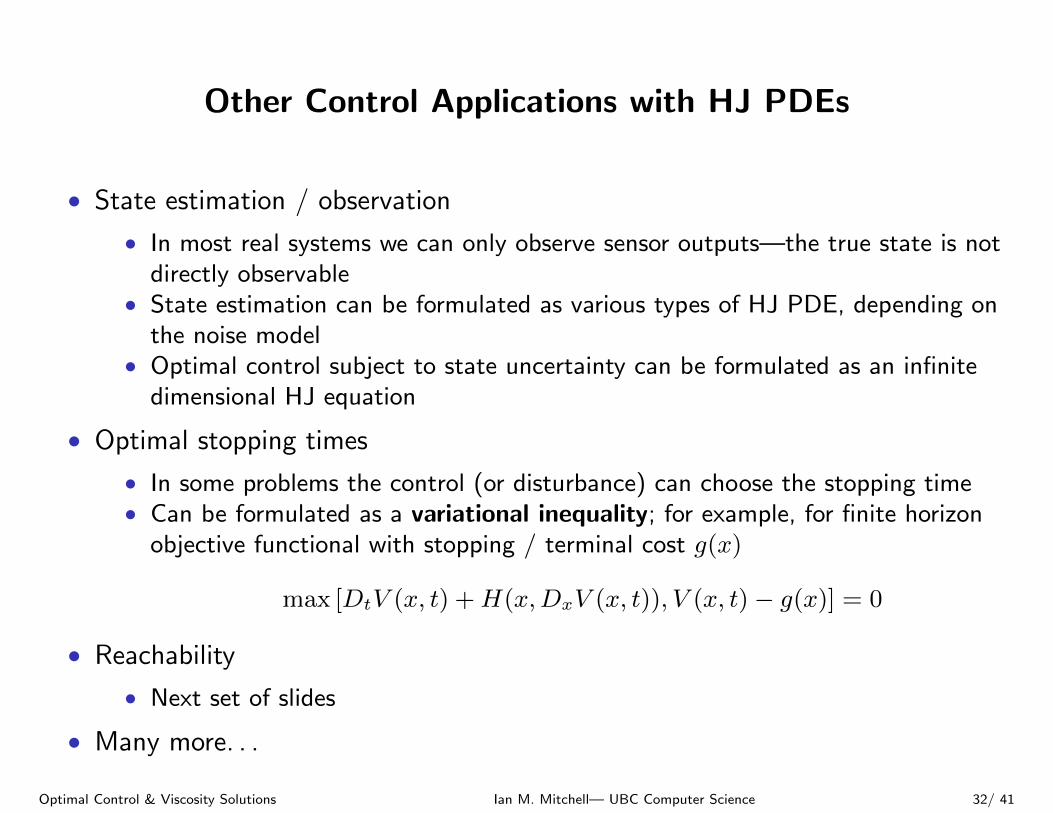
Other Control Applications with HJ PDEs
∙ State estimation / observation
∙ In most real systems we can only observe sensor outputs—the true state is notdirectly observable
∙ State estimation can be formulated as various types of HJ PDE, depending onthe noise model
∙ Optimal control subject to state uncertainty can be formulated as an infinitedimensional HJ equation
∙ Optimal stopping times
∙ In some problems the control (or disturbance) can choose the stopping time∙ Can be formulated as a variational inequality; for example, for finite horizon
objective functional with stopping / terminal cost g(x)
max [DtV (x, t) +H(x,DxV (x, t)), V (x, t)− g(x)] = 0
∙ Reachability
∙ Next set of slides
∙ Many more. . .
Optimal Control & Viscosity Solutions Ian M. Mitchell— UBC Computer Science 32/ 41

Outline
∙ Optimal control: models of system dynamics and objective functionals
∙ The value function and the dynamic programming principle
∙ A formal derivation of the Hamilton-Jacobi(-Bellman) equation
∙ Viscosity solutions and a rigorous derivation
∙ Other types of Hamilton-Jacobi equations in control
∙ Optimal control problems with analytic solutions
∙ References
Optimal Control & Viscosity Solutions Ian M. Mitchell— UBC Computer Science 33/ 41
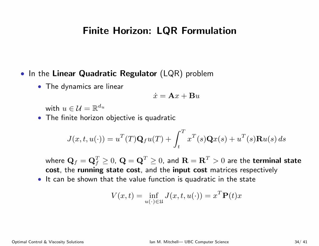
Finite Horizon: LQR Formulation
∙ In the Linear Quadratic Regulator (LQR) problem
∙ The dynamics are linearx = Ax+ Bu
with u ∈ U = ℝdu∙ The finite horizon objective is quadratic
J(x, t, u(⋅)) = uT (T )Qfu(T ) +
∫ T
t
xT (s)Qx(s) + uT (s)Ru(s) ds
where Qf = QTf ≥ 0, Q = QT ≥ 0, and R = RT > 0 are the terminal state
cost, the running state cost, and the input cost matrices respectively∙ It can be shown that the value function is quadratic in the state
V (x, t) = infu(⋅)∈U
J(x, t, u(⋅)) = xTP(t)x
Optimal Control & Viscosity Solutions Ian M. Mitchell— UBC Computer Science 34/ 41
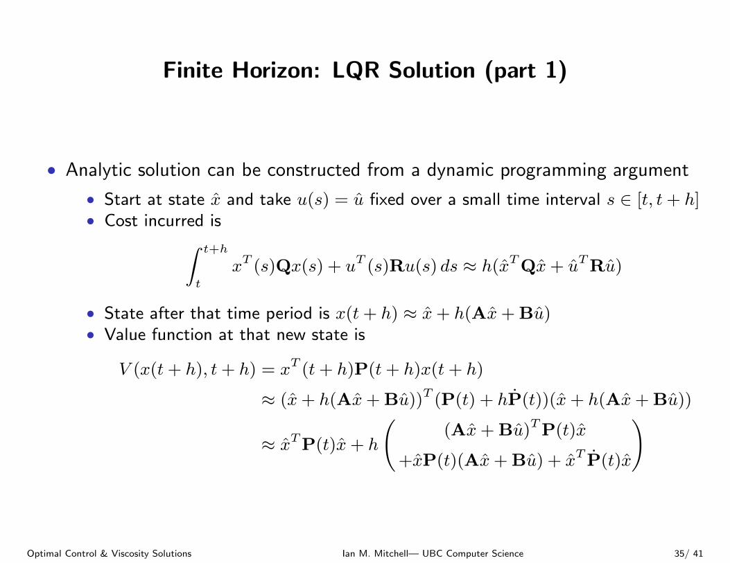
Finite Horizon: LQR Solution (part 1)
∙ Analytic solution can be constructed from a dynamic programming argument
∙ Start at state x and take u(s) = u fixed over a small time interval s ∈ [t, t+ ℎ]∙ Cost incurred is∫ t+ℎ
t
xT (s)Qx(s) + uT (s)Ru(s) ds ≈ ℎ(xTQx+ uTRu)
∙ State after that time period is x(t+ ℎ) ≈ x+ ℎ(Ax+ Bu)∙ Value function at that new state is
V (x(t+ ℎ), t+ ℎ) = xT (t+ ℎ)P(t+ ℎ)x(t+ ℎ)
≈ (x+ ℎ(Ax+ Bu))T (P(t) + ℎP(t))(x+ ℎ(Ax+ Bu))
≈ xTP(t)x+ ℎ
((Ax+ Bu)TP(t)x
+xP(t)(Ax+ Bu) + xT P(t)x
)
Optimal Control & Viscosity Solutions Ian M. Mitchell— UBC Computer Science 35/ 41
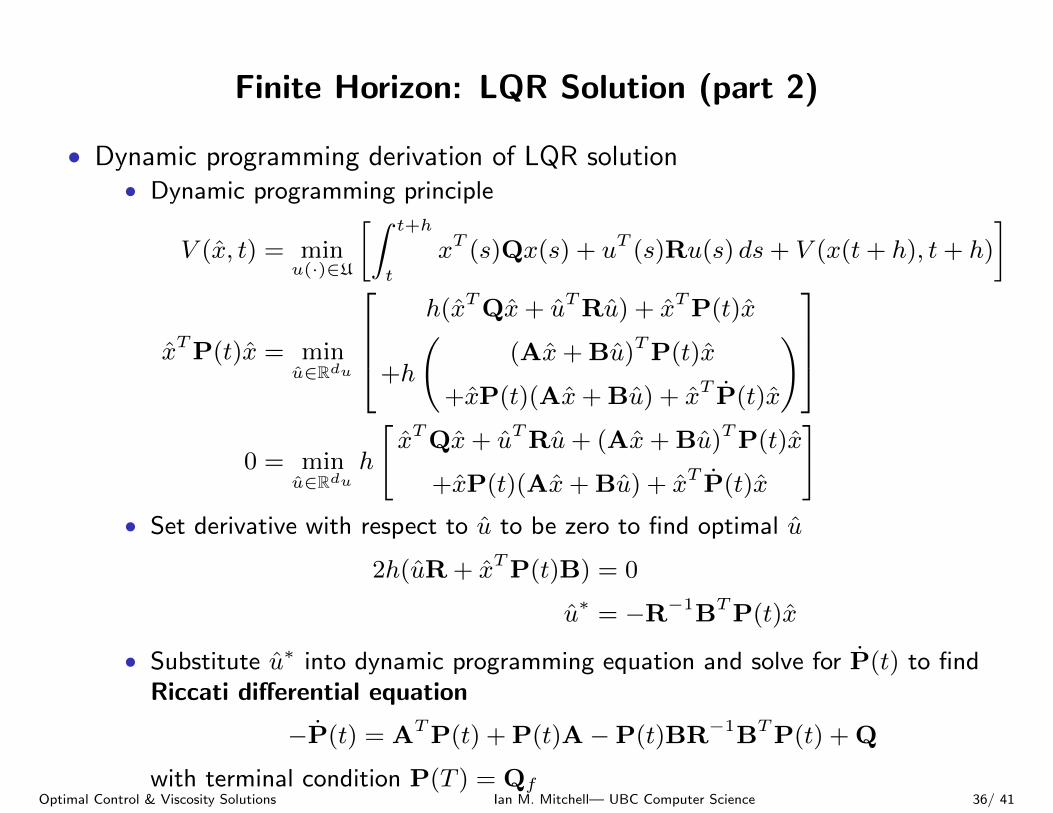
Finite Horizon: LQR Solution (part 2)
∙ Dynamic programming derivation of LQR solution∙ Dynamic programming principle
V (x, t) = minu(⋅)∈U
[∫ t+ℎ
t
xT (s)Qx(s) + uT (s)Ru(s) ds+ V (x(t+ ℎ), t+ ℎ)
]
xTP(t)x = minu∈ℝdu
⎡⎢⎢⎣ℎ(xTQx+ uTRu) + xTP(t)x
+ℎ
((Ax+ Bu)TP(t)x
+xP(t)(Ax+ Bu) + xT P(t)x
)⎤⎥⎥⎦0 = min
u∈ℝduℎ
[xTQx+ uTRu+ (Ax+ Bu)TP(t)x
+xP(t)(Ax+ Bu) + xT P(t)x
]∙ Set derivative with respect to u to be zero to find optimal u
2ℎ(uR + xTP(t)B) = 0
u∗ = −R−1BTP(t)x
∙ Substitute u∗ into dynamic programming equation and solve for P(t) to findRiccati differential equation
−P(t) = ATP(t) + P(t)A−P(t)BR−1BTP(t) + Q
with terminal condition P(T ) = QfOptimal Control & Viscosity Solutions Ian M. Mitchell— UBC Computer Science 36/ 41
(In)Finite Horizon: Steady State LQR
∙ In conclusion: LQR value function is V (x, t) = xTP(t)x where P(t) is thesolution to a terminal value (matrix) ODE
∙ In practice, P(t) and u∗ rapidly converge to steady state values
∙ Solve (continuous time) algebraic Riccati equation for steady state P
ATP + PA−PBR−1BTP + Q = 0
∙ Time-independent state feedback given by
u(t) = Kx(t) where K = −R−1BTP
∙ See Stanford’s EE363: Linear Dynamical Systems (Stephen Boyd)http://www.stanford.edu/class/ee363/
∙ This and several more derivations given in lecture notes 4 (Continuous LQR)∙ Other lectures discuss discrete time, Kalman filter (eg: LQR for state
estimation), . . .
∙ See any textbook on “state space” / “modern” control
Optimal Control & Viscosity Solutions Ian M. Mitchell— UBC Computer Science 37/ 41
Minimum Time: Double Integrator
∙ The double integrator is one of the simplest systems which is not STLC
∙ System states are position x1 and velocity x2, and the input is the accelerationu ∈ U = [−1,+1]
f(x, u) =
[x2u
]∙ If target is the origin
V (x) =
⎧⎨⎩x2 +
√4x1 + 2x2
2, if x1 >12x2∣x2∣;
−x2 +√−4x1 + 2x2
2, if x1 <12x2∣x2∣;
∣x2∣, if x1 <12x2∣x2∣
∙ Dynamics are small time controllable at the origin, so value function iscontinuous, but not Lipschitz continuous
∙ Optimal trajectories / characteristics travel along the curve where Lipschitzcontinuity fails
∙ If target set is not a circle, value function is discontinuous
∙ See Optimal Control, Athans & Falb (1966) or Applied Optimal Control,Bryson & Ho (1975) or many others
Optimal Control & Viscosity Solutions Ian M. Mitchell— UBC Computer Science 38/ 41
Known Solutions for More Complex Dynamics (part 1)
∙ Unicycle model:
x =
⎡⎣x1
x2
�
⎤⎦ x =
⎡⎣v cos �v sin �!
⎤⎦where (x1, x2) is position in the plane, � is heading, v is linear velocity and !is angular velocity
∙ Dubins’ car: Unicycle with fixed positive linear velocity and bounded angularvelocity
∙ Alternative viewpoint: unicycle with minimum turn radius∙ Minimum time to reach is generally discontinuous∙ Extensive study of combinatorial aspects of optimal paths in robotics literature:
optimal paths include CCC or CSC forms, where C is a minimum radius left orright arc of a circle (possibly of zero length) and S is a straight segment
∙ For example, see Bui, Boissonnat, Soueres & Laumond, “Shortest PathSynthesis for Dubins Non-holonomic Robot,” ICRA 1994
Optimal Control & Viscosity Solutions Ian M. Mitchell— UBC Computer Science 39/ 41
Known Solutions for More Complex Dynamics (part 2)
∙ Game of two identical vehicles: Collision avoidance with two adversarialDubins’ cars
∙ Solved in relative coordinate system, so state space remains three dimensional∙ Reachability problem becomes a two player zero sum differential game becomes
a HJI PDE∙ Analytic optimal trajectories can also be enumerated and points on the
boundary of the reachable set determined∙ Optimal characteristics both converge and diverge, causing challenges for
Lagrangian approaches∙ More details in subsequent set of slides∙ See Mitchell, “Games of Two Identical Vehicles,” Stanford University
Department of Aeronautics and Astronautics Report (SUDAAR) 740 (2001).
∙ In summary, there is no shortage of toy optimal control problems with analyticsolutions
∙ On the other hand, there is no shortage of real optimal control problemswithout analytic solutions
Optimal Control & Viscosity Solutions Ian M. Mitchell— UBC Computer Science 40/ 41
Viscosity Solution & Control References
∙ Crandall & Lions (1983) original publication
∙ Crandall, Evans & Lions (1984) current formulation
∙ Evans & Souganidis (1984) for differential games
∙ Crandall, Ishii & Lions (1992) “User’s guide” for viscosity solutions ofdegenerate ellipic and parabolic equations (dense reading)
∙ Viscosity Solutions & Applications Springer Lecture Notes in Mathematics(1995), featuring Bardi, Crandall, Evans, Soner & Souganidis(Capuzzo-Dolcetta & Lions eds)
∙ Optimal Control & Viscosity Solutions of Hamilton-Jacobi-Bellman Equations,Bardi & Capuzzo-Dolcetta (1997)
∙ Partial Differential Equations, Evans (3rd ed, 2002)
Optimal Control & Viscosity Solutions Ian M. Mitchell— UBC Computer Science 41/ 41