Optimal Control with Learned Forward Models · Optimal Control with Learned Forward Models 1 Pieter Abbeel ... Racket Position Ball Velocity ... dr dx dr du T x − xˆ u

Optimal Control with Learned Forward Models

1

Pieter AbbeelUC Berkeley

Jan PetersTU Darmstadt

Thursday, May 17, 2012

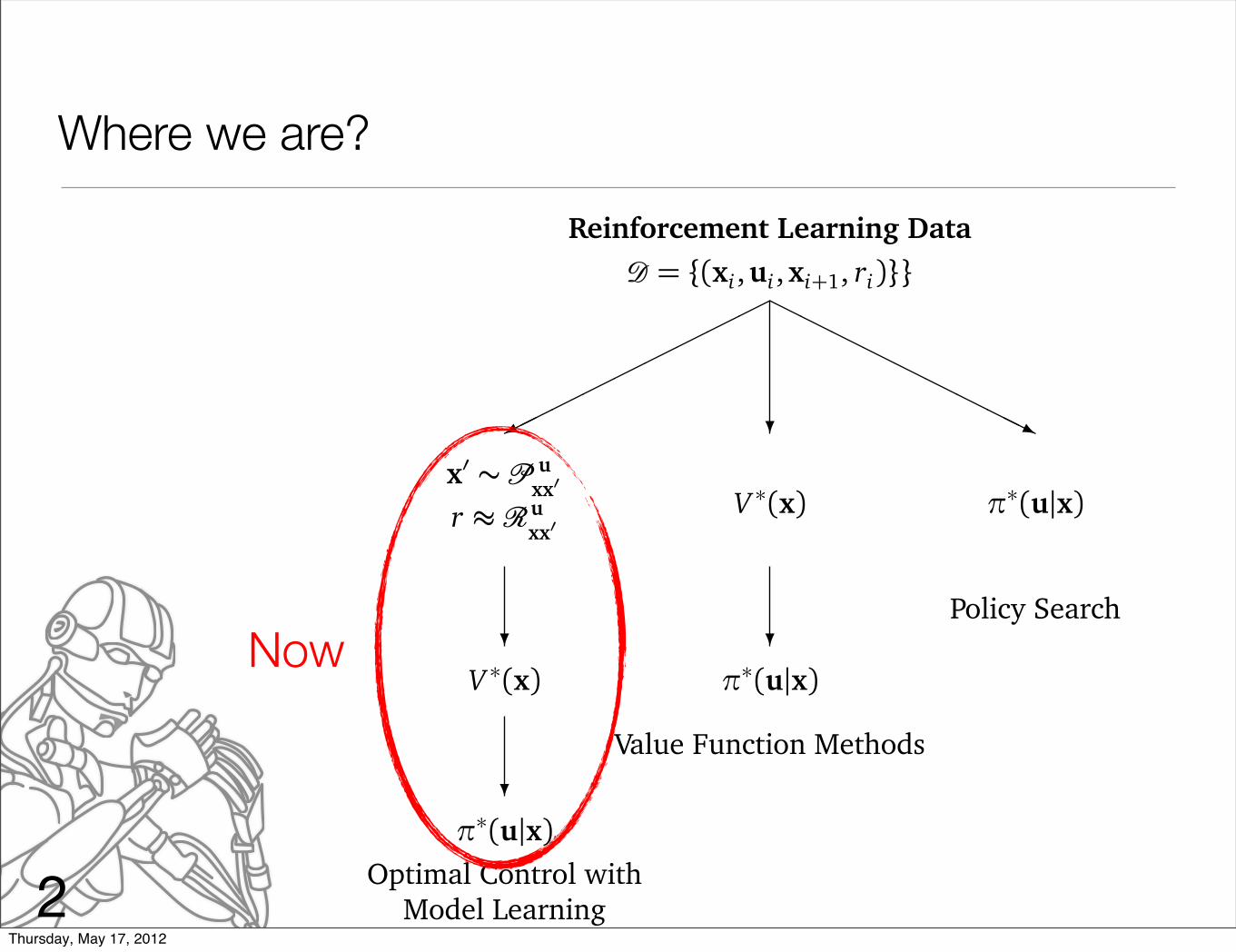
Where we are?

2

Robot Learning

Winter Semester 2011/12, ExamProf. Dr. J. Peters, M.Eng. O. Kroemer

Reminders

• Write cleanly, we cannot give you points for what we cannot read.

• You must omit exactly five questions (note: Aufgabe 1 counts as six questions). Please write OMIT on the questions

which you do not want to count. In our grading key, OMIT counts as full points for exactly five questions. Note,

if you do not use this „joker card“, we grade your answer but you can only have equal or less points. Using it is a

win-win situation.

• You are allowed two pages of handwritten notes which you submit together with your exam. Please put your name

on them.

Aufgabe 1 The Big Picture! (Equivalent to 6 Questions)

In the robot learning lecture, we covered a series of different topics. Fill in this tree...

Reinforcement Learning Data� = {(xi ,ui ,xi+1, ri)}}

✟✟✟✟✟✟✟✟✟✙

x� ∼ � uxx�

r ≈�uxx�

❄V ∗(x)

❄π∗(u|x)

Optimal Control with

Model Learning

❄

V ∗(x)

❄π∗(u|x)

Value Function Methods

❍❍❍❍❍❍❍❍❍❥

π∗(u|x)

Policy Search

1

Now


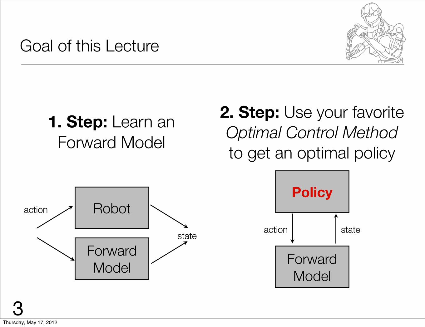
Goal of this Lecture

ForwardModel

Robotaction

state

1. Step: Learn an Forward Model

2. Step: Use your favoriteOptimal Control Methodto get an optimal policy

ForwardModel

Policy

action state

3Thursday, May 17, 2012

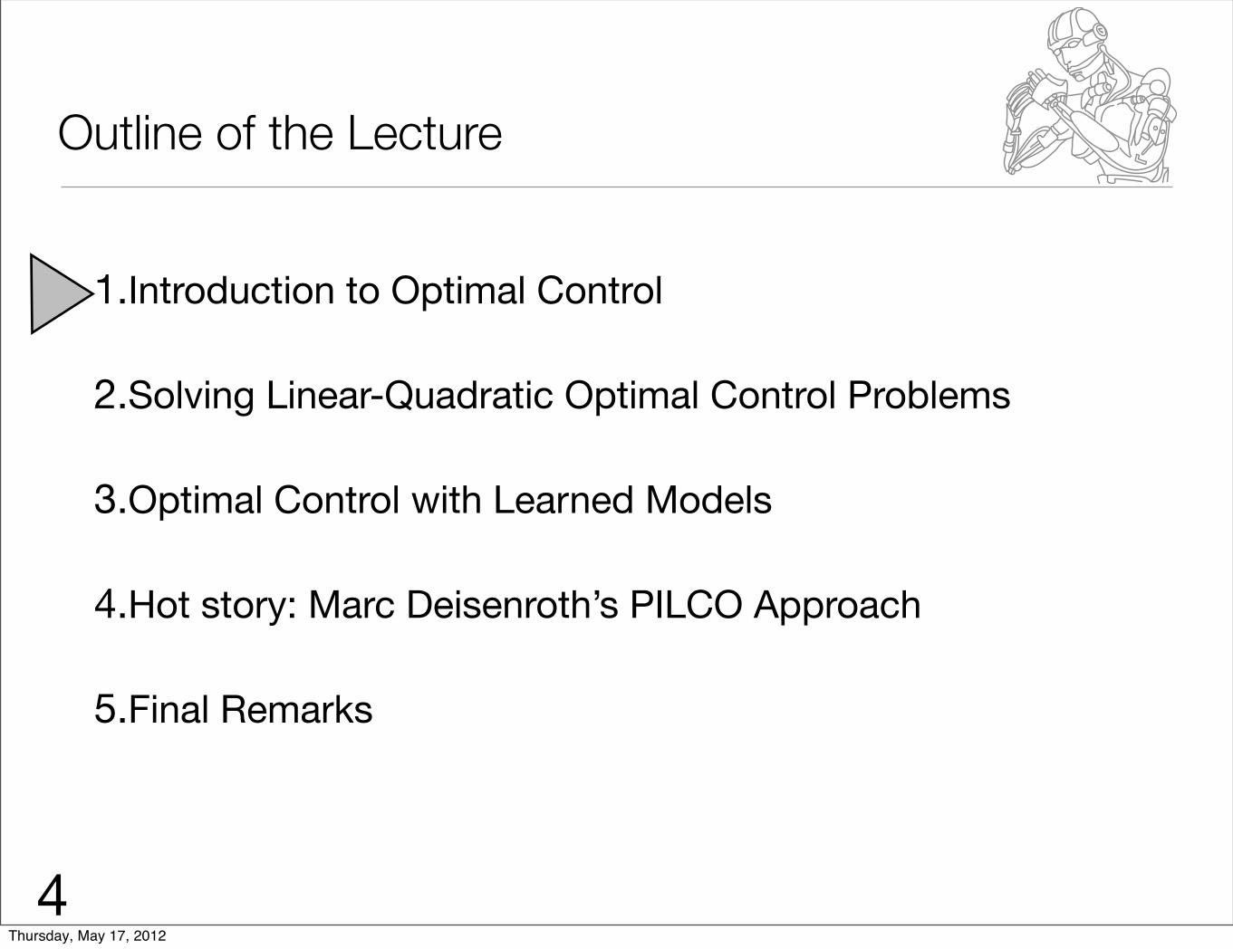
Outline of the Lecture

1.Introduction to Optimal Control

2.Solving Linear-Quadratic Optimal Control Problems

3.Optimal Control with Learned Models

4.Hot story: Marc Deisenroth’s PILCO Approach

5.Final Remarks


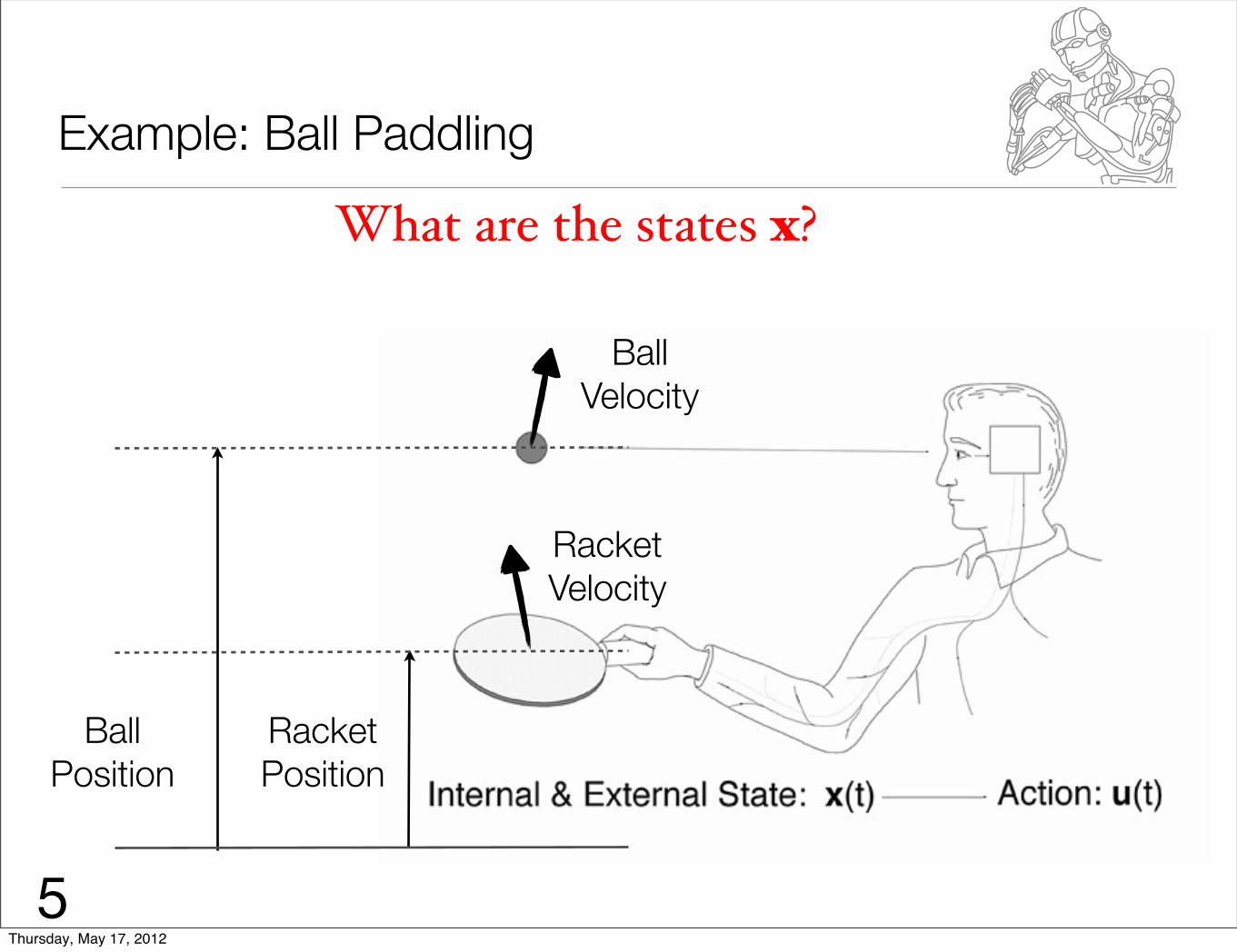
Example: Ball Paddling

What are the states x?

Racket Position

Ball Velocity

Racket Velocity

Ball Position



What are the actions u?•All motor torques?

• If you do not have a model ...

•Joint Accelerations?

• Perfect, if you have a good model ...

• Maybe identify the proper degrees of freedom?

•Accelerations in Operational Space?

• Ideally!

• ... but only if you have a good operational space control law!



What are good rewards r?•Task knowledge or success/failure?

• For some algorithms rewards in {1,0} are perfect ...

• Real problems often require reward shaping...

•What’s a good reward for our problem?

• Height of the ball?

• Distance between ball and the paddle?

• Ball needs to move in a certain region?

• All of the above?

• Additional punishments?

➡All of these together do the job!7


So can we get this to work?

•The state space has at least 12 dimensions.

•The action space has at least 3 dimensions.

•Can discretizations deal with such spaces?

•No! Finding an Optimal Value Function is limited by the curse of dimensionality.


Example: Real world application...

9

So how can you get this by RL?







5.Final Remarks


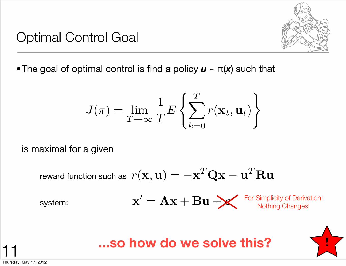
Optimal Control Goal

•The goal of optimal control is find a policy u ~ π(x) such that

is maximal for a given

reward function such as

system:

r(x,u) = −xTQx− uTRu

x� = Ax + Bu + �

...so how do we solve this?

J(π) = limT→∞

1T

E

�T�

k=0

r(xt,ut)

�

!11

For Simplicity of Derivation!Nothing Changes!


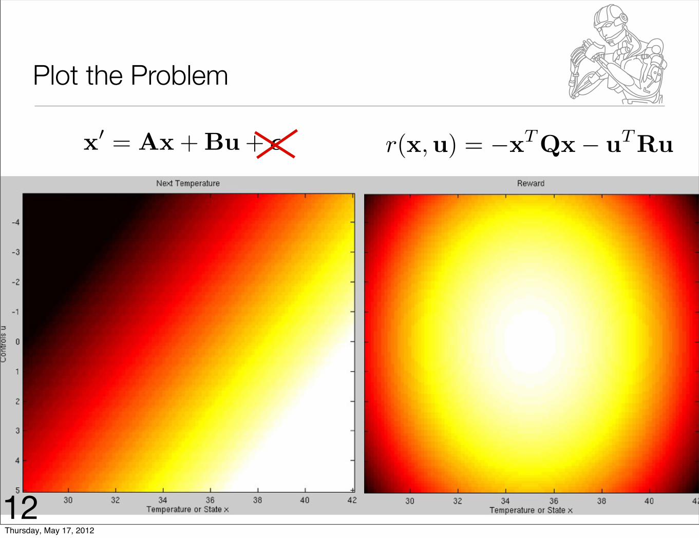
Plot the Problem

x� = Ax + Bu + � r(x,u) = −xTQx− uTRu


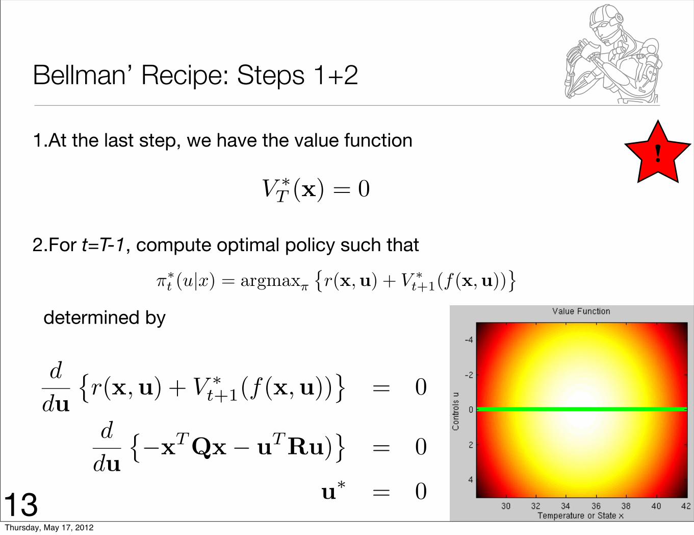
Bellman’ Recipe: Steps 1+2

1.At the last step, we have the value function

2.For t=T-1, compute optimal policy such that

determined by

V ∗T (x) = 0

π∗t (u|x) = argmaxπ

�r(x,u) + V ∗

t+1(f(x,u))�

!

d

du�r(x,u) + V ∗

t+1(f(x,u))�

= 0

d

du�−xTQx− uTRu)

�= 0

u∗ = 013Thursday, May 17, 2012

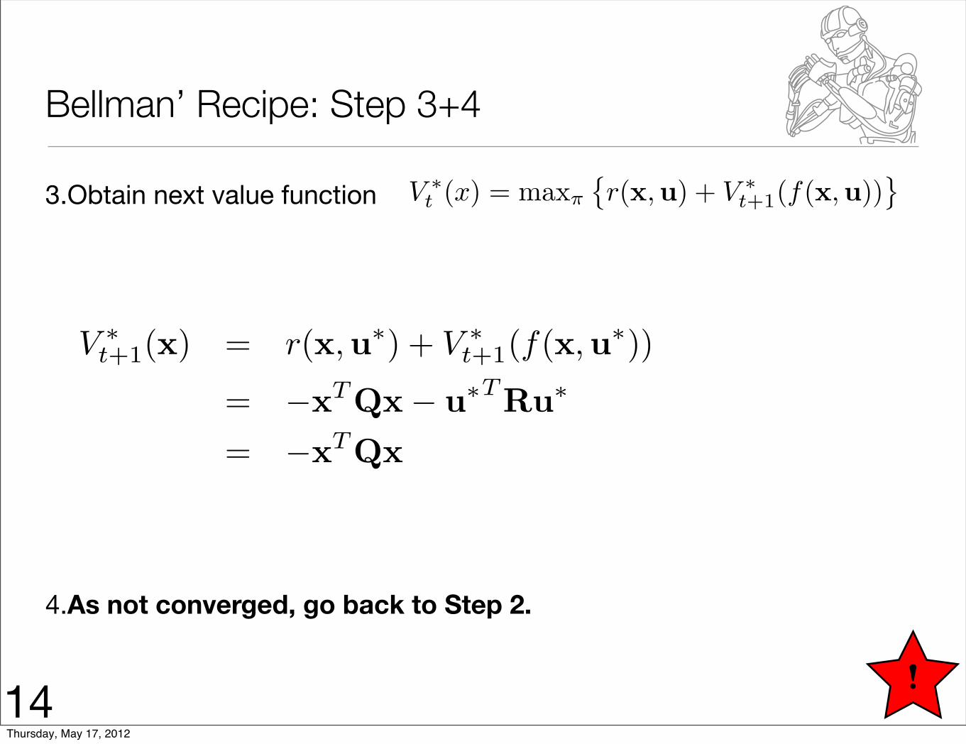
Bellman’ Recipe: Step 3+4

3.Obtain next value function

4.As not converged, go back to Step 2.

V ∗t (x) = maxπ

�r(x,u) + V ∗

t+1(f(x,u))�

V ∗t+1(x) = r(x,u∗) + V ∗

t+1(f(x,u∗))

= −xTQx− u∗TRu∗

= −xTQx

!14Thursday, May 17, 2012

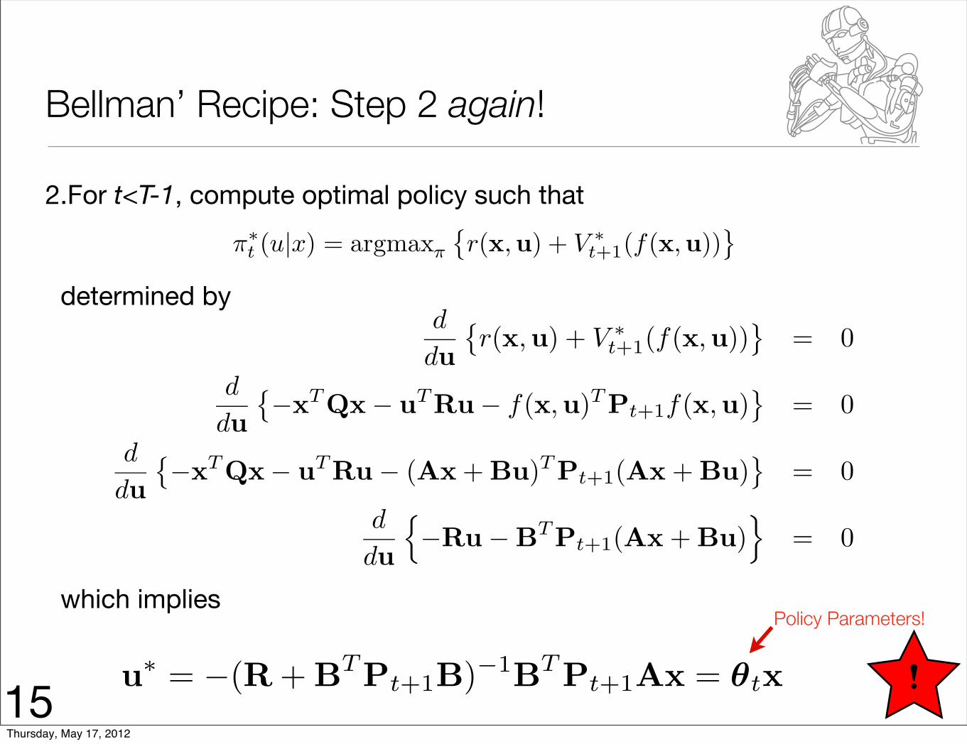
u∗ = −(R + BTPt+1B)−1BT Pt+1Ax = θtx

Bellman’ Recipe: Step 2 again!

2.For t<T-1, compute optimal policy such that

determined by

which implies


�r(x,u) + V ∗

t+1(f(x,u))�

!

Policy Parameters!

d

du�r(x,u) + V ∗

t+1(f(x,u))�

= 0

d

du�−xTQx− uTRu− f(x,u)T Pt+1f(x,u)

�= 0

d

du�−xTQx− uTRu− (Ax + Bu)T Pt+1(Ax + Bu)

�= 0

d

du

�−Ru−BTPt+1(Ax + Bu)

�= 0


Pt = −Q− θTt+1Rθt+1 − (A + Bθt+1)T Pt+1 + (A + Bθt+1)

θt = −(R + BTPt+1B)−1BTPt+1A

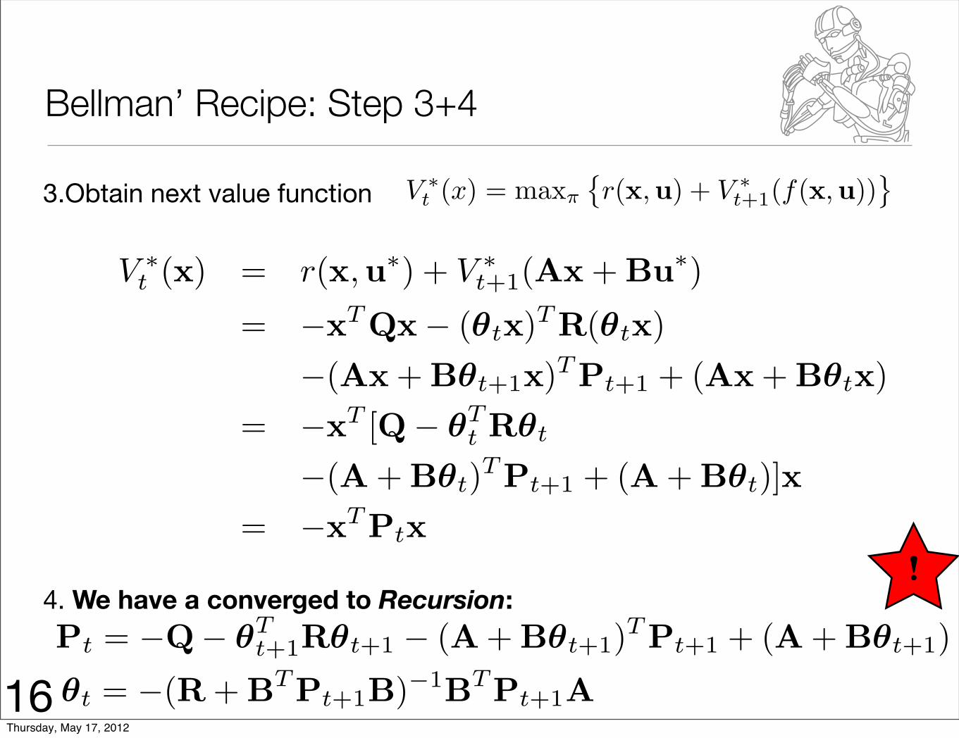
Bellman’ Recipe: Step 3+4


4. We have a converged to Recursion:

V ∗t (x) = maxπ

�r(x,u) + V ∗

t+1(f(x,u))�

!

V ∗t (x) = r(x,u∗) + V ∗

t+1(Ax + Bu∗)

= −xT Qx− (θtx)T R(θtx)−(Ax + Bθt+1x)T Pt+1 + (Ax + Bθtx)

= −xT [Q− θTt Rθt

−(A + Bθt)T Pt+1 + (A + Bθt)]x= −xT Ptx


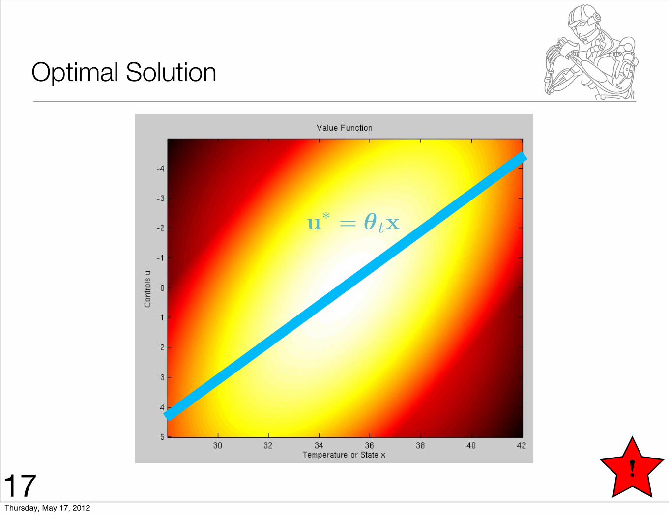
Optimal Solution

u∗ = θtx

!17Thursday, May 17, 2012






5.Final Remarks


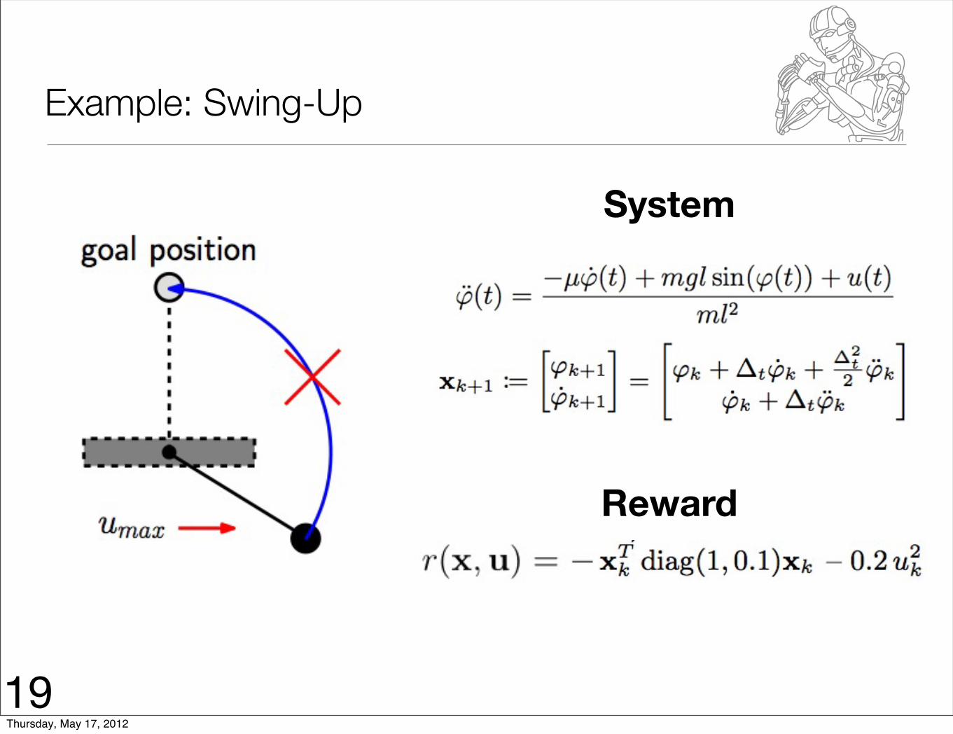
Example: Swing-Up

System

Reward


Possible: Learn Solutions only where needed!

If you know places where

we start...

... we can just look ahead!

20 Atkeson & Schaal, 1995Thursday, May 17, 2012

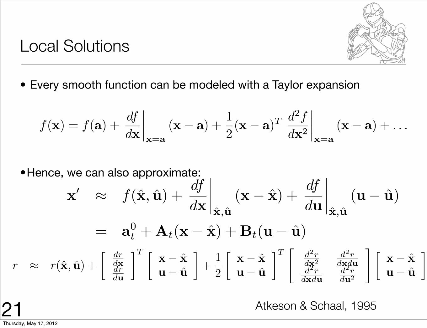
Local Solutions

• Every smooth function can be modeled with a Taylor expansion

•Hence, we can also approximate:

f(x) = f(a) +df

dx

��x=a

(x− a) +12(x− a)T d2f

dx2

��x=a

(x− a) + . . .

r ≈ r(x, u) +�

drdxdrdu

�T �x− xu− u

�+

12

�x− xu− u

�T�

d2rdx2

d2rdxdu

d2rdxdu

d2rdu2

��x− xu− u

�

x� ≈ f(x, u) +df

dx

��x,u

(x − x) +df

du

��x,u

(u− u)

= a0t + At(x− x) + Bt(u− u)

21 Atkeson & Schaal, 1995Thursday, May 17, 2012

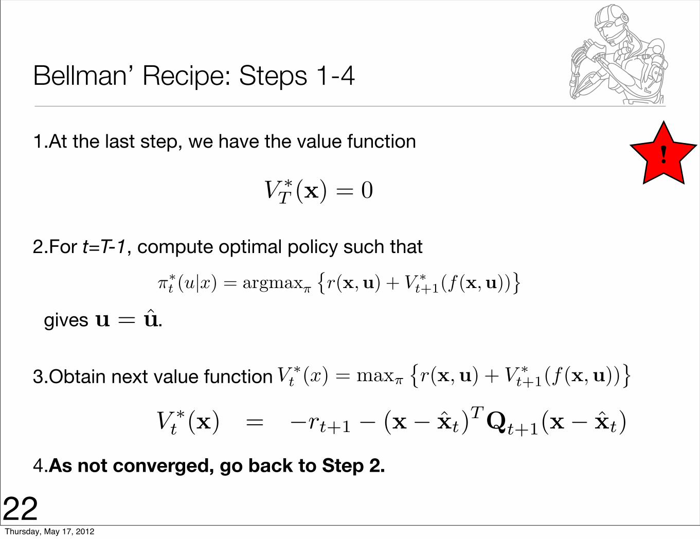
Bellman’ Recipe: Steps 1-4

1.At the last step, we have the value function

2.For t=T-1, compute optimal policy such that

gives .


4.As not converged, go back to Step 2.

V ∗T (x) = 0


�r(x,u) + V ∗

t+1(f(x,u))�

!

u = u

V ∗t (x) = maxπ

�r(x,u) + V ∗

t+1(f(x,u))�

V ∗t (x) = −rt+1 − (x− xt)TQt+1(x− xt)


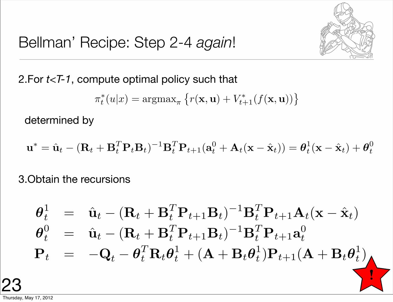
Bellman’ Recipe: Step 2-4 again!

2.For t<T-1, compute optimal policy such that

determined by

3.Obtain the recursions


�r(x,u) + V ∗

t+1(f(x,u))�

!

θ1t = ut − (Rt + BT

t Pt+1Bt)−1BTt Pt+1At(x − xt)

θ0t = ut − (Rt + BT

t Pt+1Bt)−1BTt Pt+1a0

t

Pt = −Qt − θTt Rtθ

1t + (A + Btθ

1t )Pt+1(A + Btθ

1t )

u∗ = ut − (Rt + BTt PtBt)−1BT

t Pt+1(a0t + At(x− xt)) = θ1

t (x− xt) + θ0t


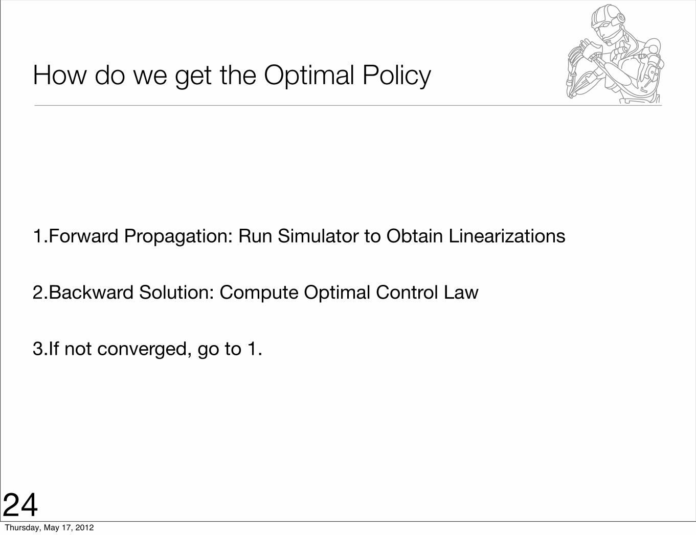
How do we get the Optimal Policy

1.Forward Propagation: Run Simulator to Obtain Linearizations

2.Backward Solution: Compute Optimal Control Law

3.If not converged, go to 1.


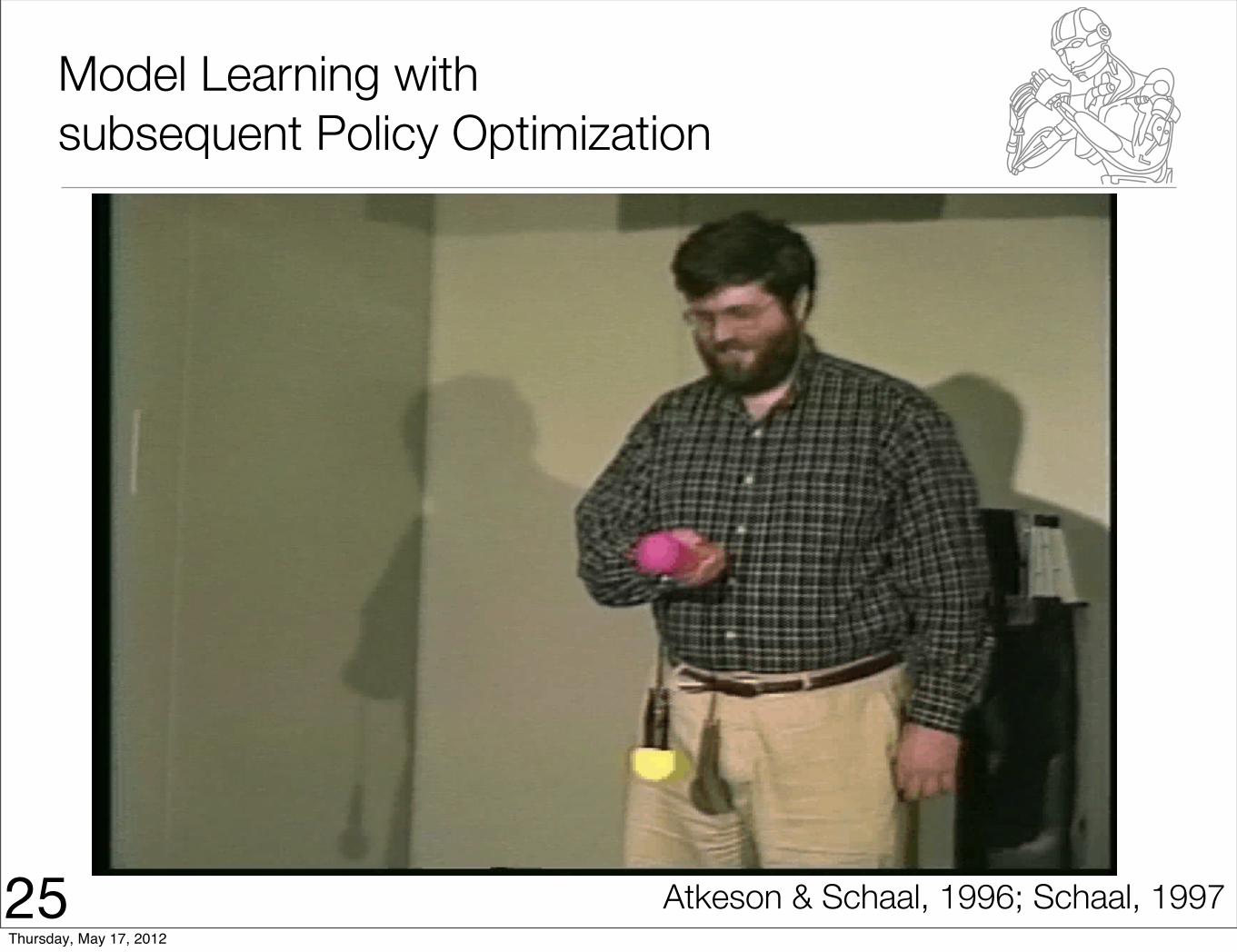
Model Learning with subsequent Policy Optimization

25 Atkeson & Schaal, 1996; Schaal, 1997Thursday, May 17, 2012

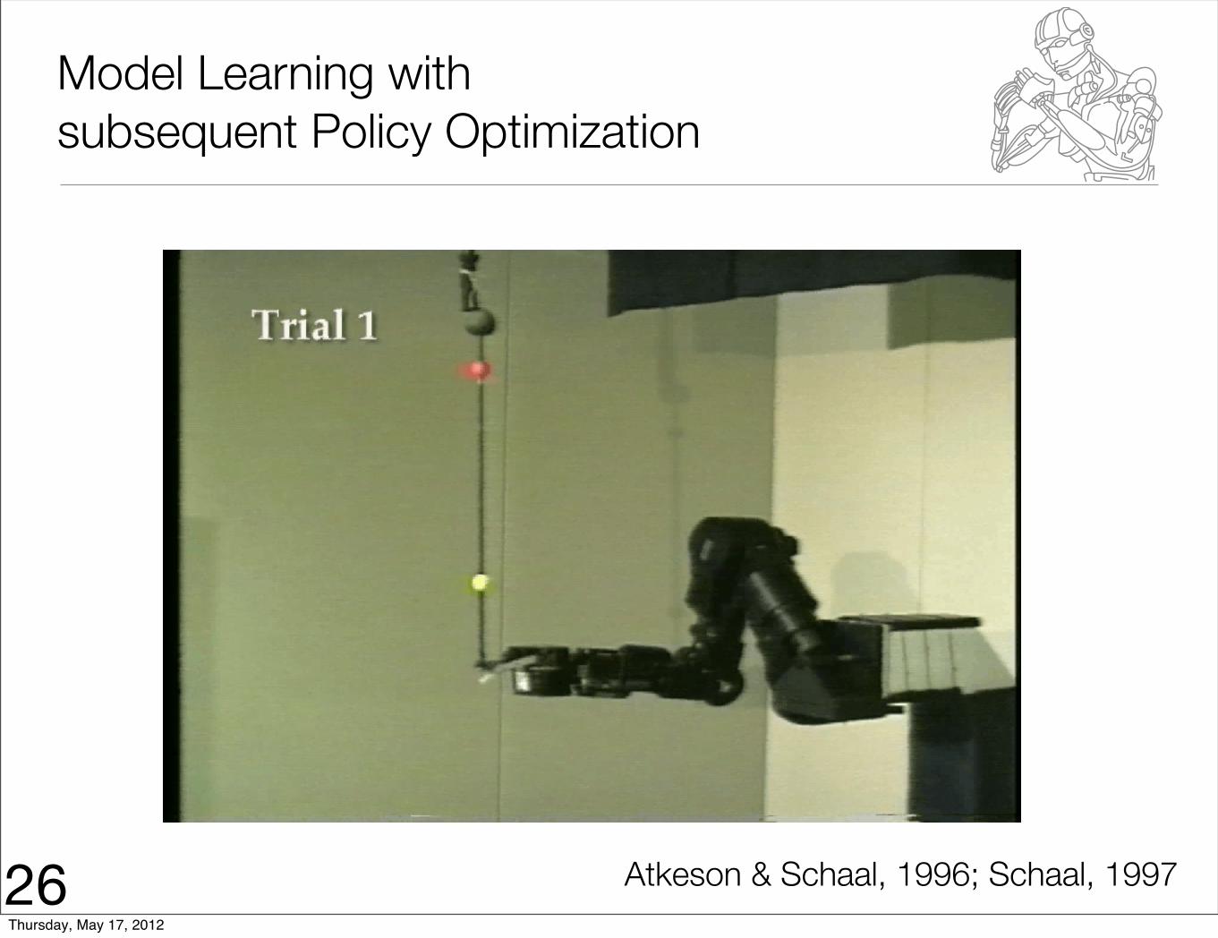
Model Learning with subsequent Policy Optimization

26 Atkeson & Schaal, 1996; Schaal, 1997Thursday, May 17, 2012






5.Final Remarks


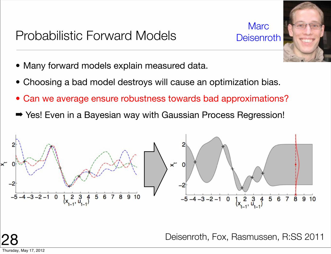
Probabilistic Forward Models

• Many forward models explain measured data.

• Choosing a bad model destroys will cause an optimization bias.

• Can we average ensure robustness towards bad approximations?

➡ Yes! Even in a Bayesian way with Gaussian Process Regression!

28

Marc Deisenroth

Deisenroth, Fox, Rasmussen, R:SS 2011Thursday, May 17, 2012

Basic Idea

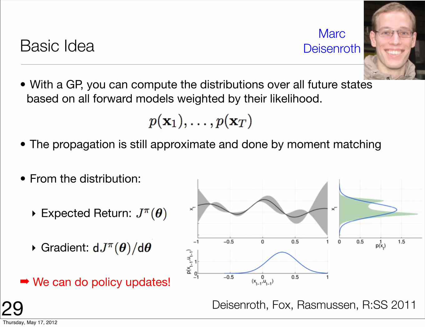
• With a GP, you can compute the distributions over all future states based on all forward models weighted by their likelihood.

• The propagation is still approximate and done by moment matching

• From the distribution:

‣ Expected Return:

‣ Gradient:

➡ We can do policy updates!

29

Marc Deisenroth


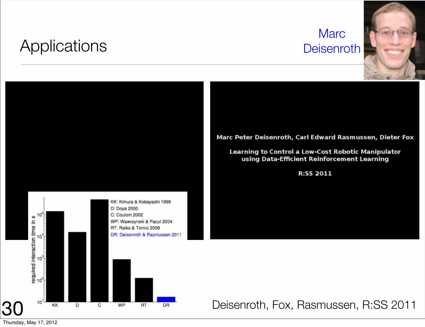
Applications

30

Marc Deisenroth







5.Final Remarks


Conclusions

•You have learned about optimal control today!

•Only two cased are solvable: linear & discrete!•Linear scales but does not generalize.•Discrete generalizes but does not scale.

•Using Learned Models, you can compute at least optimal “policy tubes”.

•If you have many many tubes, in good regions, you have a policy.

•We will continue with Value Function and Policy Search Methods.


Further Reading

•C. G. Atkeson (1994), Using Local Trajectory Optimizers to Speed Up Global Optimization in Dynamic Programming, Proceedings, Neural Information Processing Systems, Denver, Colorado, December, 1993, In: Neural Information Processing Systems 6, J. D. Cowan, G. Tesauro, and J. Alspector, eds. Morgan Kaufmann, 1994.

• Schaal, S. (1997). “Learning from demonstration”. In: M.C. Mozer, M. Jordan, & T. Petsche (eds.), Advances in Neural Information Processing Systems 9, pp.1040-1046. Cambridge, MA: MIT Press

•Marc P. Deisenroth, Carl E. Rasmussen, Dieter Fox (2011). Learning to Control a Low-Cost Robotic Manipulator Using Data-Efficient Reinforcement Learning, Robotics: Science & Systems (RSS 2011)


http://www.cs.cmu.edu/~cga/papers/local.pdf




Documents

Optimal Control with Learned Forward Models · Optimal Control with Learned Forward Models 1 Pieter Abbeel ... Racket Position Ball Velocity ... dr dx dr du T x − xˆ u