Embed Size (px)
Citation preview
Optimal Energy Harvesting from Vortex-Induced Vibrations of Cables
Guillaume O. Antoine, Emmanuel de Langre, and Sebastien Michelin∗
LadHyX – Departement de Mecanique, Ecole Polytechnique – CNRS, 91128 Palaiseau, France.(Dated: October 18, 2016)
Vortex-induced vibrations (VIV) of flexible cables are an example of flow-induced vibrations thatcan act as energy harvesting systems by converting energy associated with the spontaneous cablemotion into electricity. This work investigates the optimal positioning of the harvesting devices alongthe cable, using numerical simulations with a wake oscillator model to describe the unsteady flowforcing. Using classical gradient-based optimization, the optimal harvesting strategy is determinedfor the generic configuration of a flexible cable fixed at both ends, including the effect of flow forcesand gravity on the cable’s geometry. The optimal strategy is found to consist systematically in aconcentration of the harvesting devices at one of the cable’s ends, relying on deformation waves alongthe cable to carry the energy toward this harvesting site. Furthermore, we show that the performanceof systems based on VIV of flexible cables is significantly more robust to flow velocity variations, incomparison with a rigid cylinder device. This results from two passive control mechanisms inherentto the cable geometry : (i) the adaptability to the flow velocity of the fundamental frequencies ofcables through the flow-induced tension and (ii) the selection of successive vibration modes by theflow velocity for cables with gravity-induced tension.
2
I. INTRODUCTION
The field of renewable energies is gaining interest due to the limited availability and the environmental impact offossil fuels. Flow-induced vibrations, i.e. the motion of a solid structure resulting from the destabilizing effect of forcesapplied by the surrounding flow, have recently received an increased attention as a potential alternative to classicalwind- and water-turbines to convert a fraction of the fluid’s kinetic energy into electricity [1].
From an energy point of view, flow-induced vibrations transfer a fraction of the kinetic energy of the incomingflow to the solid structure that is set into motion. Vibrations can then be used to power an electric generator andeffectively convert some of the solid’s mechanical energy into electrical form. Recently, many classical examples offlow-induced vibrations have been revisited as potential energy harvesting mechanisms, including galloping [2–6],coupled-mode flutter of airfoil profiles [7], flutter of flexible cylinders or membranes in axial flow [8–11], flapping inunsteady wakes [12–15] and vortex-induced vibrations (VIV) of rigid and flexible structures [1, 16–22]. The presentwork focuses on the possibility to harvest energy from VIV of long flexible cables.
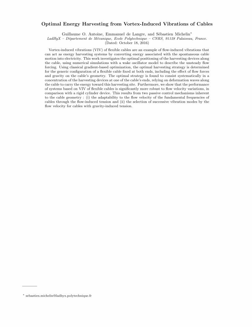
VIV result from the coupling of a bluff body to its unsteady vortex wake. The steady flow around a fixed bluff bodyat high Reynolds number (Re � 1 or inertial flows) is characterized by an unsteady shedding of vortex structures.The wake structure is then complex and differs from a classical Von-Karman vortex street observed at lower Re, butits frequency spectrum is still dominated by a fundamental frequency known as the Strouhal frequency f , proportionalto the flow velocity U as f = ST U/D with ST the Strouhal frequency and D the diameter (e.g. [23, 24]). This resultsin an unsteady lift force on the bluff body. For a flexible or flexibly-mounted structure (see Fig. 1), this unsteadyforce will force the solid body into so-called vortex-induced vibrations, and this unsteady motion of the body will alsointroduce a feedback coupling on the vortex shedding and unsteady lift. VIV of a rigid cylinder mounted on an elasticfoundation have been widely studied, both experimentally and numerically (see [23–26]. A distinctive feature of VIVis the lock-in mechanism: when the fundamental frequency of the solid’s vibrations is close to the Strouhal frequency,the coupling between the vibrations and the vortex shedding synchronizes both dynamics over an extended range offlow velocity. This results in self-sustained, self-limited large amplitude oscillations of the solid, typically of the orderof one cross-flow diameter.
This lock-in phenomenon is particularly interesting for energy harvesting purposes since large amplitudes imply thatthe oscillating structure has a large amount of kinetic energy that can potentially be harnessed to produce electricity.The VIVACE system [1] relies on that phenomenon.
However, VIV of elastically-mounted rigid cylinders also have intrinsic limitations. Lock-in occurs only when theStrouhal frequency and the eigenfrequency of the structure are sufficiently close, e.g. [24]. If this condition is not met(“lock-out”), the rigid cylinder is not properly excited by the flow and its oscillations have negligible amplitude, whichresults in inefficient energy extraction. Geophysical flows (e.g. oceanic, tidal or river currents) are characterized by animportant variability in the flow velocity magnitude, and systems relying on VIV of rigid cylinders can only produceenergy when the flow velocity remains close to the velocity for which they are designed.
u u
FIG. 1. Vortex-induced vibrations of a rigid cylinder (left) and a flexible cable (right) in a steady and uniform cross flow.
A method to circumvent this issue is to use flexible structures (cables, or beams) rather than rigid cylinders, assketched in Fig. 1: cables have multiple deformation modes which have their own eigenfrequencies and different modescan be locked-in for different values of the flow velocity (and Strouhal frequency). The selective excitation of a specificdeformation mode of a flexible structure when the eigenfrequency of the latter is close to the Strouhal frequency wasdemonstrated experimentally [27, 28] and numerically [29]. Rather than lock-out, variations of the flow velocityinduce a transition towards lock-in of higher or lower deformation modes. This advantage of flexible structures wasrecently demonstrated for a system consisting of a hanging cable in a cross flow, attached to a local energy harvesterat its upper end [21]. The experimental and numerical results obtained for that system demonstrated its increasedrobustness to variations in the flow velocity in comparison with an elastically supported rigid system.
A challenge and open question associated with harvesting energy from VIV of flexible structures is to determine theoptimal harvesting strategy, i.e. where and how the mechanical energy of the solid structure should be converted into

3
O
u
re
Ye
Xe
Ze
e
e
FIG. 2. VIV of a flexible cable. The inset shows the definition of the local orthonormal basis (er, eθ, eϕ).
electricity. With a rigid cylinder, the motion is a pure translation with a single degree of freedom, and determiningthe optimal strategy is relatively simple. For flexible structures, the periodic motion is not uniform throughout thestructure, which results in a much larger configuration space for the harvesting distribution. Optimization of such asystem is a particular challenge. Moreover, the geometry of the structure and how it is held in the flow are additionaldesign variables. The present work addresses these questions and investigates the optimal route to efficient energyharvesting using VIV of flexible cables.
The paper is organized as follows. Section II presents the mathematical and numerical models used here to analysethe VIV dynamics and resulting energy harvesting. In Section III, the distribution of harvesting devices on a flexiblecable is optimized, and the performance of such system is analysed and compared to the reference rigid system inSection IV. Section V finally summarizes the main conclusions of our work, stressing out both its fundamental andengineering implications.
II. MODEL FOR THE VIV OF HANGING CABLES
A. Problem geometry
In this work, we consider a long inextensible cable of circular cross-section with density ρS , length L and diameterD with a large aspect ratio Λ = L/D � 1, see Fig. 2; its extremities O and O′ are fixed and aligned along eX ata distance ∆L from each other. By “cable” (or equivalently “string”) we mean that the structure has no bendingstiffness, thus the only structural force is the tension force which acts as a Lagrangian multiplier that enforces theinextensibility condition. The reader is referred to Ref. [30] for a thorough description of the string model. The cableis immersed in a uniform horizontal cross flow u = ueY .
The dynamics of the cable are the result of a balance between the cable’s inertia, the internal tension, gravityand buoyancy, and flow forces. We focus on vortex-induced vibrations (VIV) for which the cable undergoes smalloscillations about a steady mean position as a result of the unsteady vortex shedding on the structure.
Flow forces on the moving structure can be modelled as the superposition of four different components [31, 32]: (i)
a drag force1
2ρCDD|ur⊥|ur⊥, (ii) a friction force
π
2ρCFD|ur|ur‖, (iii) an added mass and (iv) an unsteady lift force
resulting from periodic vortex shedding in the structure’s wake. Here, ρ is the mass density of the fluid and ur = u− xis the local relative velocity of the incoming flow to the cable whose position is noted x(s, t), and (ur‖,u
r⊥) are its
components along and normal to the cable, respectively.
In the following, the problem is written in non-dimensional form by choosing L, 1/(2πf) and1
2ρCDU
2DL as
characteristic length, time and force, respectively.
B. Mean Position of the Structure
We first focus on the mean (i.e. time-averaged) steady position of the cable, obtained by balancing the effects ofthe steady fluid forces, the cable’s weight, buoyancy and the internal tension (inertia, added-mass and wake effects
4
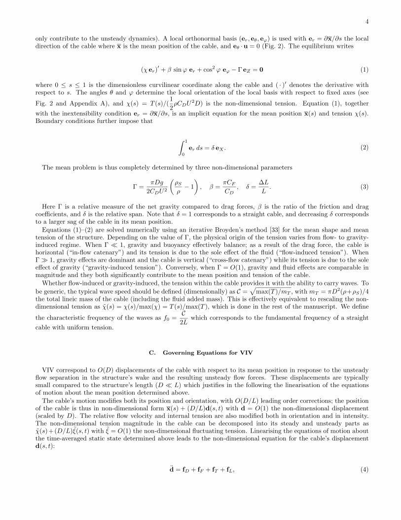
only contribute to the unsteady dynamics). A local orthonormal basis (er, eθ, eϕ) is used with er = ∂x/∂s the localdirection of the cable where x is the mean position of the cable, and eθ ·u = 0 (Fig. 2). The equilibrium writes
(χ er)′+ β sinϕ er + cos2 ϕ eϕ − Γ eZ = 0 (1)
where 0 ≤ s ≤ 1 is the dimensionless curvilinear coordinate along the cable and ( · )′ denotes the derivative withrespect to s. The angles θ and ϕ determine the local orientation of the local basis with respect to fixed axes (see
Fig. 2 and Appendix A), and χ(s) = T (s)/(1
2ρCDU
2D) is the non-dimensional tension. Equation (1), together
with the inextensibility condition er = ∂x/∂s, is an implicit equation for the mean position x(s) and tension χ(s).Boundary conditions further impose that
∫ 1
0
er ds = δ eX . (2)
The mean problem is thus completely determined by three non-dimensional parameters
Γ =πDg
2CDU2
(ρSρ− 1
), β =
πCFCD
, δ =∆L
L. (3)
Here Γ is a relative measure of the net gravity compared to drag forces, β is the ratio of the friction and dragcoefficients, and δ is the relative span. Note that δ = 1 corresponds to a straight cable, and decreasing δ correspondsto a larger sag of the cable in its mean position.
Equations (1)–(2) are solved numerically using an iterative Broyden’s method [33] for the mean shape and meantension of the structure. Depending on the value of Γ, the physical origin of the tension varies from flow- to gravity-induced regime. When Γ � 1, gravity and buoyancy effectively balance; as a result of the drag force, the cable ishorizontal (“in-flow catenary”) and its tension is due to the sole effect of the fluid (“flow-induced tension”). WhenΓ� 1, gravity effects are dominant and the cable is vertical (“cross-flow catenary”) while its tension is due to the soleeffect of gravity (“gravity-induced tension”). Conversely, when Γ = O(1), gravity and fluid effects are comparable inmagnitude and they both significantly contribute to the mean position and tension of the cable.
Whether flow-induced or gravity-induced, the tension within the cable provides it with the ability to carry waves. To
be generic, the typical wave speed should be defined (dimensionally) as C =√
max(T )/mT , with mT = πD2(ρ+ρS)/4the total lineic mass of the cable (including the fluid added mass). This is effectively equivalent to rescaling the non-dimensional tension as χ(s) = χ(s)/max(χ) = T (s)/max(T ), which is done in the rest of the manuscript. We define
the characteristic frequency of the waves as f0 =C
2Lwhich corresponds to the fundamental frequency of a straight
cable with uniform tension.
C. Governing Equations for VIV
VIV correspond to O(D) displacements of the cable with respect to its mean position in response to the unsteadyflow separation in the structure’s wake and the resulting unsteady flow forces. These displacements are typicallysmall compared to the structure’s length (D � L) which justifies in the following the linearisation of the equationsof motion about the mean position determined above.
The cable’s motion modifies both its position and orientation, with O(D/L) leading order corrections; the positionof the cable is thus in non-dimensional form x(s) + (D/L)d(s, t) with d = O(1) the non-dimensional displacement(scaled by D). The relative flow velocity and internal tension are also modified both in orientation and in intensity.The non-dimensional tension magnitude in the cable can be decomposed into its steady and unsteady parts asχ(s)+(D/L)ξ(s, t) with ξ = O(1) the non-dimensional fluctuating tension. Linearising the equations of motion aboutthe time-averaged static state determined above leads to the non-dimensional equation for the cable’s displacementd(s, t):
d = fD + fF + fT + fL, (4)

5
where ˙( ) denotes the time derivative, and the fluctuating drag, friction and tension forces are obtained as
fD = −γµ
cosϕ(dθ eθ + 2 dϕ eϕ
)(5)
fF = −β γµ
(dr + sinϕ eY · d
)er, (6)
fT =1
π2u2
(χ′ d′ + χd′′ + ξ′ er + ξ e′r
)(7)
with (dr, dθ, dϕ) the components of d in the local basis, and u, γ and µ, respectively defined as the reduced velocity(or frequency ratio), damping and mass ratios [21, 29, 34]
u =f
f0= 2ST
L
D
U
C, γ =
CD4πST
, µ =π
4
(1 +
ρSρ
). (8)
The inextensibility of the cable further imposes that d′ · er = 0.The effect of the unsteady wake on the structure is modelled here as a fluctuating lift force fL which is orthogonal
to both the direction of the flow and the axis of the cable. As shown by Franzini et al. [35], vortex shedding is mostlygoverned by the flow orthogonal to the cable’s axis and, consequently, the lift force is quadratic in the normal relativeflow velocity (i.e. |ur⊥|2) with a local fluctuating lift coefficient CL0
q(s, t)/2 (with CL0the lift coefficient of a still
cylinder [34]), so that in Eq. (4), fL is given by
fL = M q(s, t) cos2 ϕ eθ, with M =CL0
16π2µS2T
· (9)
So-called wake oscillator models describe the dynamics of this fluctuating lift as a nonlinear van der Pol oscillatorforced by the motion of the structure in order to account for the feedback coupling of solid motion on vortex shedding,which is an essential ingredient to lock-in. Previous studies have shown that a local inertial coupling leads to a goodagreement with experimental and numerical studies on rigid and flexible structures in VIV [29, 34, 36, 37]. Thedynamics of the wake variable q(s, t) are then governed by
q + ε cosϕ(q2 − 1
)q + cos2 ϕ q = A dθ. (10)
The values of the non-dimensional parameters ε and A of the wake oscillator model need to be determined usingexperimental (or numerical) data. More details about this model for the wake effects and validation against experi-mental data for the VIV of rigid cylinders and straight strings are provided in [29, 34].
In this work, unless stated otherwise, the following numerical values are used for the parameters of the model:ST = 0.17, CL0 = 0.61, CD = 2.0, CF = 0.083, ε = 0.3 and A = 12 (e.g. [34]). Two different values of µ are usedin the paper: µ = 2.79, which is consistent with previous works on the topic (e.g. [21, 29, 34]), and µ = π/2 ≈ 1.57,which corresponds to a neutrally buoyant cable.
The extremities of the cable are fixed, which yields the boundary conditions d|s=0 = d|s=1 = 0. Equations (4)–(7),(9) and (10) are numerically integrated in time starting from an initial state where the cable is at rest in its meanposition (d(t = 0) = 0) while the wake is given a small perturbation (at t = 0, q = q0(s)� 1 and q = 0) that triggersthe oscillations of the system which eventually reaches a steady oscillatory regime that does not depend on the choiceof initial conditions.
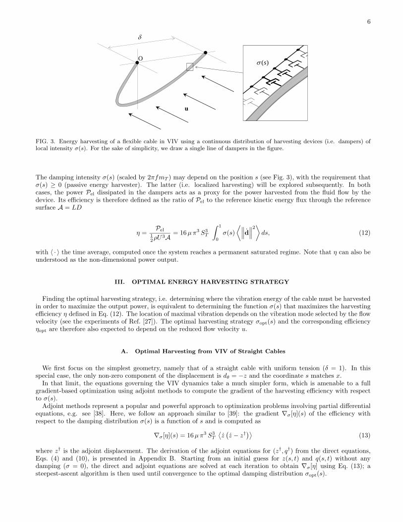
D. Modeling Energy Harvesting
This work focuses on the possibility of harvesting energy from a flow using the cable’s VIV, and on the optimalstrategy to maximize the energy output. Energy harvesting amounts to converting some of the energy associated withthe vibrations into a usable form – typically electricity. As it effectively removes some mechanical energy from thestructure, energy harvesting must be modelled explicitly in order to properly account for its effect on the vibrationitself. The simplest model is that of a pure linear damping force. This damping can be either distributed (i.e. presentall along the structure) or localized at some position along the cable. The former will be our initial focus, andcorresponds to an additional non uniform damping force fH in the equations of motion of the cable, Eq. (4):
fH = −σ(s) d. (11)
6
)(sO
u
FIG. 3. Energy harvesting of a flexible cable in VIV using a continuous distribution of harvesting devices (i.e. dampers) oflocal intensity σ(s). For the sake of simplicity, we draw a single line of dampers in the figure.
The damping intensity σ(s) (scaled by 2πfmT ) may depend on the position s (see Fig. 3), with the requirement thatσ(s) ≥ 0 (passive energy harvester). The latter (i.e. localized harvesting) will be explored subsequently. In bothcases, the power Pel dissipated in the dampers acts as a proxy for the power harvested from the fluid flow by thedevice. Its efficiency is therefore defined as the ratio of Pel to the reference kinetic energy flux through the referencesurface A = LD
η =Pel
12ρU
3A= 16µπ3 S3
T
∫ 1
0
σ(s)
⟨∥∥∥d∥∥∥2⟩ ds, (12)
with 〈 · 〉 the time average, computed once the system reaches a permanent saturated regime. Note that η can also beunderstood as the non-dimensional power output.
III. OPTIMAL ENERGY HARVESTING STRATEGY
Finding the optimal harvesting strategy, i.e. determining where the vibration energy of the cable must be harvestedin order to maximize the output power, is equivalent to determining the function σ(s) that maximizes the harvestingefficiency η defined in Eq. (12). The location of maximal vibration depends on the vibration mode selected by the flowvelocity (see the experiments of Ref. [27]). The optimal harvesting strategy σopt(s) and the corresponding efficiencyηopt are therefore also expected to depend on the reduced flow velocity u.
A. Optimal Harvesting from VIV of Straight Cables
We first focus on the simplest geometry, namely that of a straight cable with uniform tension (δ = 1). In thisspecial case, the only non-zero component of the displacement is dθ = −z and the coordinate s matches x.
In that limit, the equations governing the VIV dynamics take a much simpler form, which is amenable to a fullgradient-based optimization using adjoint methods to compute the gradient of the harvesting efficiency with respectto σ(s).
Adjoint methods represent a popular and powerful approach to optimization problems involving partial differentialequations, e.g. see [38]. Here, we follow an approach similar to [39]: the gradient ∇σ[η](s) of the efficiency withrespect to the damping distribution σ(s) is a function of s and is computed as
∇σ[η](s) = 16µπ3 S3T
⟨z(z − z†
)⟩(13)
where z† is the adjoint displacement. The derivation of the adjoint equations for (z†, q†) from the direct equations,Eqs. (4) and (10), is presented in Appendix B. Starting from an initial guess for z(s, t) and q(s, t) without anydamping (σ = 0), the direct and adjoint equations are solved at each iteration to obtain ∇σ[η] using Eq. (13); asteepest-ascent algorithm is then used until convergence to the optimal damping distribution σopt(s).
7
(a)
(b)
(c)
(d)
1u
z
yx
2u
z
yx
x
t/2π
0 0.2 0.4 0.6 0.8 1
0
0.5
1
1.5
2 −1
−0.5
0
0.5
1
x
t/2π
0 0.2 0.4 0.6 0.8 1
0
0.5
1
1.5
2 −1
−0.5
0
0.5
1
0 0.2 0.4 0.6 0.8 10
0.05
0.1
0.15
0.2
0.25
x
Optimaldampingdistrib.σopt
0 0.2 0.4 0.6 0.8 10
0.05
0.1
0.15
0.2
0.25
x
Optimaldampingdistrib.σopt
x
t/2π
0 0.2 0.4 0.6 0.8 1
0
0.5
1
1.5
2 −0.5
−0.25
0
0.25
0.5
x
t/2π
0 0.2 0.4 0.6 0.8 1
0
0.5
1
1.5
2 −0.5
−0.25
0
0.25
0.5
Figure 1: Straight cable in mode 1, from top to bottom: initial y-contours, optimal σ distribution, final y-contours
1
x
t/2π
0 0.2 0.4 0.6 0.8 1
0
0.5
1
1.5
2 −1
−0.5
0
0.5
1
x
t/2π
0 0.2 0.4 0.6 0.8 1
0
0.5
1
1.5
2 −1
−0.5
0
0.5
1
0 0.2 0.4 0.6 0.8 10
0.1
0.2
0.3
0.4
0.5
x
Optimaldampingdistrib.σopt
0 0.2 0.4 0.6 0.8 10
0.1
0.2
0.3
0.4
0.5
x
Optimaldampingdistrib.σopt
x
t/2π
0 0.2 0.4 0.6 0.8 1
0
0.5
1
1.5
2 −0.5
−0.25
0
0.25
0.5
x
t/2π
0 0.2 0.4 0.6 0.8 1
0
0.5
1
1.5
2 −0.5
−0.25
0
0.25
0.5
Figure 1: Straight cable in mode 2, from top to bottom: initial y-contours, optimal σ distribution, final y-contours
1
Figure 1: Straight cable in modes 1 (left) and 2 (right), from top to bottom: initial y-contours, optimal σ distribu-tions, final y-contours
1
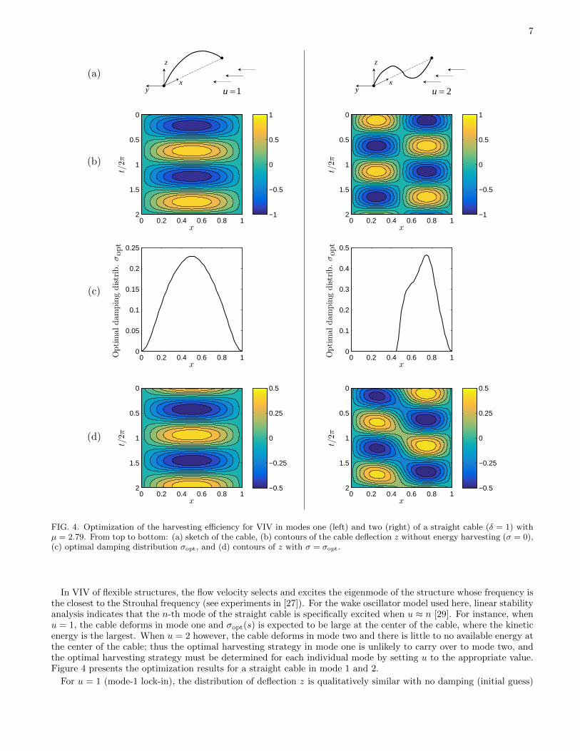
FIG. 4. Optimization of the harvesting efficiency for VIV in modes one (left) and two (right) of a straight cable (δ = 1) withµ = 2.79. From top to bottom: (a) sketch of the cable, (b) contours of the cable deflection z without energy harvesting (σ = 0),(c) optimal damping distribution σopt, and (d) contours of z with σ = σopt.
In VIV of flexible structures, the flow velocity selects and excites the eigenmode of the structure whose frequency isthe closest to the Strouhal frequency (see experiments in [27]). For the wake oscillator model used here, linear stabilityanalysis indicates that the n-th mode of the straight cable is specifically excited when u ≈ n [29]. For instance, whenu = 1, the cable deforms in mode one and σopt(s) is expected to be large at the center of the cable, where the kineticenergy is the largest. When u = 2 however, the cable deforms in mode two and there is little to no available energy atthe center of the cable; thus the optimal harvesting strategy in mode one is unlikely to carry over to mode two, andthe optimal harvesting strategy must be determined for each individual mode by setting u to the appropriate value.Figure 4 presents the optimization results for a straight cable in mode 1 and 2.
For u = 1 (mode-1 lock-in), the distribution of deflection z is qualitatively similar with no damping (initial guess)
8
and with an optimal damping (final result). The amplitude of the oscillations with the optimal harvesting strategyis nearly half that of the oscillations without energy harvesting, indicating a significant energy extraction from theoscillations. The optimal damping distribution σopt respects the mode one symmetry.
For u = 2 (mode-2 lock-in), the distribution of deflection z without damping (initial guess) corresponds to a mode-two deformation – which validates our criterion n = u. This is not the case for the z-contours in the optimal-dampingsituation: the optimal strategy corresponds to a non-symmetric damping distribution σopt(s) (Fig. 4), for which mostof the energy extraction occurs on one half of the cable. Progressive waves carry energy from the undamped part ofthe cable to the harvesting location. The optimal efficiency is similar for u = 1 and u = 2, with ηopt = 8.1% andηopt = 8.6%, respectively.
These results are in fact generic: for any n ≥ 2, the optimization algorithm leads to an optimal strategy withharvesting concentrated on a reduced fraction of the cable near one of its fixed ends, while the rest of the cable isundamped, and energy is carried to the harvesting region by travelling waves along the cable.
Those results are particularly relevant from a practical and engineering point of view: regardless of the selectedmode except mode 1 (and therefore for any sufficiently large velocity), the optimal strategy consists in restrictingthe harvesting system to a limited fraction of the cable near one of its attachment points, rather than distributing italong the entire cable.
B. Optimal Harvesting from VIV of Catenary Cables
We can extend the previous approach and results to the general configuration of Fig. 3. The optimal harvestingstrategy σopt(s) now depends on three parameters: δ and Γ, that set the mean position of the cable, and u, whichsets the vibration mode of the cable excited by the flow. Assuming a piecewise constant damping σ(s), the dampingdistribution σopt(s) is computed for different values of (δ,Γ, u) using a steepest-ascent algorithm, now computing thegradient numerically.
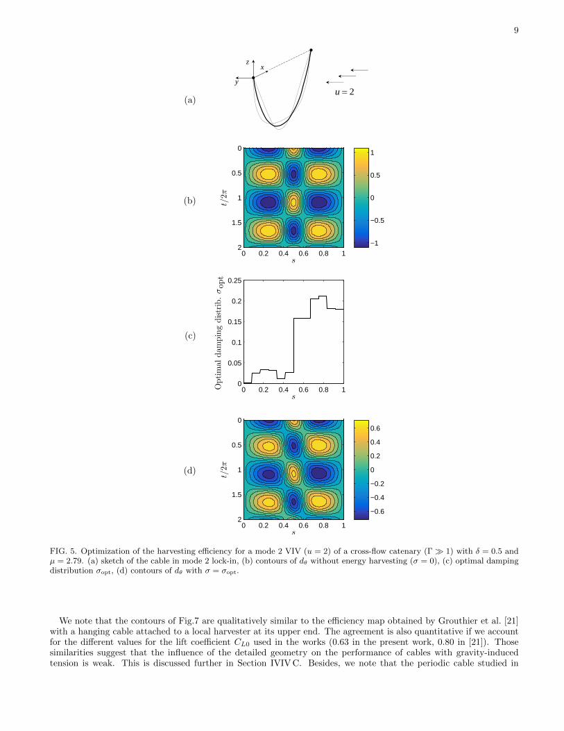
Figure 5 shows the optimal distribution of damping and resulting dynamics obtained for a cross-flow catenarycable (ηopt = 7.6%). As for the straight cable, the optimal damping distribution is not symmetric and waves areobserved to carry energy toward the harvesting site. This behaviour is in fact observed for all geometries providedthe excited mode number is greater than 2. This generality therefore suggests to go one step further and investigatethe performance of harvesting energy at a single point located at the extremity of the cable rather than in its vicinity.
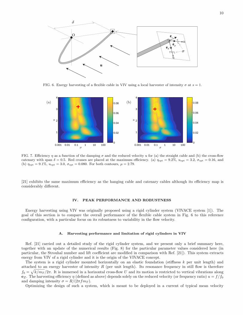
C. Local Point-Wise Damper as Optimal Harvesting Strategy
To this end, the fixed boundary condition at s = 1 is now relaxed to allow for transverse displacements of the cableand energy extraction. More precisely, at s = 1, the cable can slide in the local (θ,ϕ) plane and energy harvesting ismodelled as a linear viscous force resisting its velocity with a damping intensity σ (Fig. 6). Note that σ is a scalarvalue here. The cable and wake dynamics are still governed by Eqs. (4) and (10) (without an additional damping force)and the boundary condition at s = 1 now balances local tension and viscous forces (the fixed boundary condition ats = 0 remains unchanged):
dr = 0 , d′ · eθ + π2u2 σ dθ = 0 , d′ · eϕ + π2u2 σ dϕ = 0 (14)
The harvesting efficiency of this system is still defined as the ratio of the average power dissipated in the damper tothe kinetic energy flux through the area occupied by the cable:
η = 16µπ3 S3T σ
⟨∥∥∥ d∣∣∣s=1
∥∥∥2⟩ (15)
The optimization now consists in maximizing η with respect to the scalar parameter σ.For a given geometry (i.e. given δ and Γ), the optimal damping strategy and efficiency are determined by directly
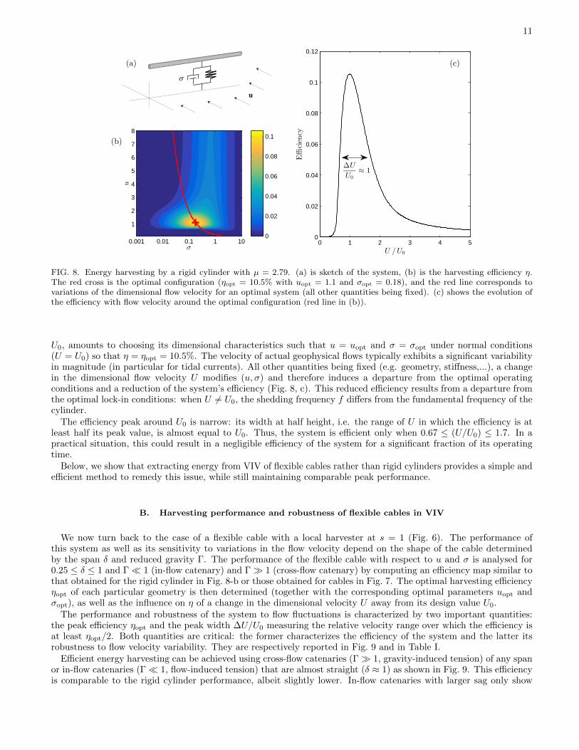
computing η(u, σ) and finding its absolute maximum. Figure 7 shows the evolution of η(u, σ) for the configurationsof Figs. 4 (straight cable) and 5 (catenary).
The maximum efficiency for the straight cable and the cross-flow catenary is slightly more than 9%, which exceedsthe maximum performance obtained with distributed harvesters: the local harvesting strategy is therefore optimalfor both configurations. This finding is again generic, and valid for most geometries: for δ ranging between 0.25 and1 and Γ � 1, Γ ∼ 1 and Γ � 1 we find that the optimal efficiency of a local damper is equivalent or slightly higherthan the optimal efficiency of distributed damping.
9
(a)2u
z
y
x
(b)
(c)
(d)
s
t/2π
0 0.2 0.4 0.6 0.8 1
0
0.5
1
1.5
2−1
−0.5
0
0.5
1
s
t/2π
0 0.2 0.4 0.6 0.8 1
0
0.5
1
1.5
2−1
−0.5
0
0.5
1
0 0.2 0.4 0.6 0.8 10
0.05
0.1
0.15
0.2
0.25
s
Optimaldampingdistrib.σopt
0 0.2 0.4 0.6 0.8 10
0.05
0.1
0.15
0.2
0.25
s
Optimaldampingdistrib.σopt
s
t/2π
0 0.2 0.4 0.6 0.8 1
0
0.5
1
1.5
2−0.6
−0.4
−0.2
0
0.2
0.4
0.6
s
t/2π
0 0.2 0.4 0.6 0.8 1
0
0.5
1
1.5
2−0.6
−0.4
−0.2
0
0.2
0.4
0.6
Figure 1: Heavy cable with span 0.50 in mode 2, from top to bottom: initial dθ-contours, optimal σ distribution,final dθ-contours
1
Figure 1: Heavy cable with δ=0.5 in mode 2, from top to bottom: initial dθ-contours, optimal σ distributions, finaldθ-contours
1
FIG. 5. Optimization of the harvesting efficiency for a mode 2 VIV (u = 2) of a cross-flow catenary (Γ � 1) with δ = 0.5 andµ = 2.79. (a) sketch of the cable in mode 2 lock-in, (b) contours of dθ without energy harvesting (σ = 0), (c) optimal dampingdistribution σopt, (d) contours of dθ with σ = σopt.
We note that the contours of Fig.7 are qualitatively similar to the efficiency map obtained by Grouthier et al. [21]with a hanging cable attached to a local harvester at its upper end. The agreement is also quantitative if we accountfor the different values for the lift coefficient CL0 used in the works (0.63 in the present work, 0.80 in [21]). Thosesimilarities suggest that the influence of the detailed geometry on the performance of cables with gravity-inducedtension is weak. This is discussed further in Section IVIV C. Besides, we note that the periodic cable studied in
10
O
u
re
ee
FIG. 6. Energy harvesting of a flexible cable in VIV using a local harvester of intensity σ at s = 1.
σ
u
0.001 0.01 0.1 1 10 100
1
2
3
4
0
0.02
0.04
0.06
0.08
σ
u
0.001 0.01 0.1 1 10 100
1
2
3
4
0
0.02
0.04
0.06
0.08(a) (b)
Figure 1: η vs. u and σ. Left: straight cable; Right: heavy cable w/ δ = 0.5. For both: µ = 2.79. Left:uopt/π = 3.2, σopt = 9.17% = 0.16, ηopt = 9.17% ; Right: uopt/π = 3.0, σopt = 9.17% = 0.080, ηopt = 9.06%
1
FIG. 7. Efficiency η as a function of the damping σ and the reduced velocity u for (a) the straight cable and (b) the cross-flowcatenary with span δ = 0.5. Red crosses are placed at the maximum efficiency. (a) ηopt = 9.2%, uopt = 3.2, σopt = 0.16, and(b) ηopt = 9.1%, uopt = 3.0, σopt = 0.080. For both contours, µ = 2.79.
[21] exhibits the same maximum efficiency as the hanging cable and catenary cables although its efficiency map isconsiderably different.
IV. PEAK PERFORMANCE AND ROBUSTNESS
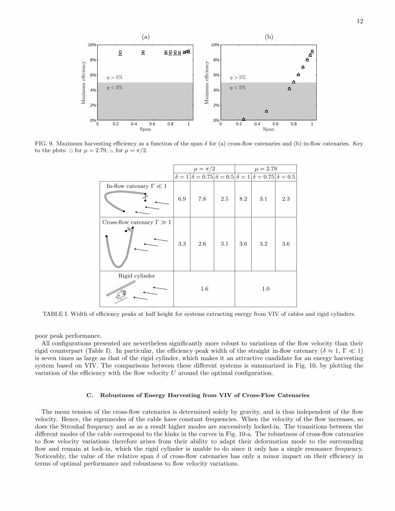
Energy harvesting using VIV was originally proposed using a rigid cylinder system (VIVACE system [1]). Thegoal of this section is to compare the overall performance of the flexible cable system in Fig. 6 to this referenceconfiguration, with a particular focus on its robustness to variability in the flow velocity.
A. Harvesting performance and limitation of rigid cylinders in VIV
Ref. [21] carried out a detailed study of the rigid cylinder system, and we present only a brief summary here,together with an update of the numerical results (Fig. 8) for the particular parameter values considered here (inparticular, the Strouhal number and lift coefficient are modified in comparison with Ref. [21]). This system extractsenergy from VIV of a rigid cylinder and it is the origin of the VIVACE concept.
The system is a rigid cylinder mounted horizontally on an elastic foundation (stiffness k per unit length) andattached to an energy harvester of intensity R (per unit length). Its resonance frequency in still flow is therefore
f0 =√k/mT /2π. It is immersed in a horizontal cross-flow U and its motion is restricted to vertical vibrations along
eZ . The harvesting efficiency η (defined as above) depends solely on the reduced velocity (or frequency ratio) u = f/f0and damping intensity σ = R/(2πfmT ).
Optimizing the design of such a system, which is meant to be deployed in a current of typical mean velocity
11
u
σ
u
0.001 0.01 0.1 1 10
1
2
3
4
5
6
7
8
0
0.02
0.04
0.06
0.08
0.1
Figure 1: Extracting energy from VIVs of rigid cylinder: sketch and contours.
u
σ
u
0.001 0.01 0.1 1 10
1
2
3
4
5
6
7
8
0
0.02
0.04
0.06
0.08
0.1
0 1 2 3 4 50
0.02
0.04
0.06
0.08
0.1
0.12
U /U0
Efficiency
∆U
U0
≈ 1
(a) (c)
(b)
Figure 2: Extracting energy from VIVs of rigid cylinder: sketch, contours, and isodamping.
1
FIG. 8. Energy harvesting by a rigid cylinder with µ = 2.79. (a) is sketch of the system, (b) is the harvesting efficiency η.The red cross is the optimal configuration (ηopt = 10.5% with uopt = 1.1 and σopt = 0.18), and the red line corresponds tovariations of the dimensional flow velocity for an optimal system (all other quantities being fixed). (c) shows the evolution ofthe efficiency with flow velocity around the optimal configuration (red line in (b)).
U0, amounts to choosing its dimensional characteristics such that u = uopt and σ = σopt under normal conditions(U = U0) so that η = ηopt = 10.5%. The velocity of actual geophysical flows typically exhibits a significant variabilityin magnitude (in particular for tidal currents). All other quantities being fixed (e.g. geometry, stiffness,...), a changein the dimensional flow velocity U modifies (u, σ) and therefore induces a departure from the optimal operatingconditions and a reduction of the system’s efficiency (Fig. 8, c). This reduced efficiency results from a departure fromthe optimal lock-in conditions: when U 6= U0, the shedding frequency f differs from the fundamental frequency of thecylinder.
The efficiency peak around U0 is narrow: its width at half height, i.e. the range of U in which the efficiency is atleast half its peak value, is almost equal to U0. Thus, the system is efficient only when 0.67 ≤ (U/U0) ≤ 1.7. In apractical situation, this could result in a negligible efficiency of the system for a significant fraction of its operatingtime.
Below, we show that extracting energy from VIV of flexible cables rather than rigid cylinders provides a simple andefficient method to remedy this issue, while still maintaining comparable peak performance.
B. Harvesting performance and robustness of flexible cables in VIV
We now turn back to the case of a flexible cable with a local harvester at s = 1 (Fig. 6). The performance ofthis system as well as its sensitivity to variations in the flow velocity depend on the shape of the cable determinedby the span δ and reduced gravity Γ. The performance of the flexible cable with respect to u and σ is analysed for0.25 ≤ δ ≤ 1 and Γ� 1 (in-flow catenary) and Γ� 1 (cross-flow catenary) by computing an efficiency map similar tothat obtained for the rigid cylinder in Fig. 8-b or those obtained for cables in Fig. 7. The optimal harvesting efficiencyηopt of each particular geometry is then determined (together with the corresponding optimal parameters uopt andσopt), as well as the influence on η of a change in the dimensional velocity U away from its design value U0.
The performance and robustness of the system to flow fluctuations is characterized by two important quantities:the peak efficiency ηopt and the peak width ∆U/U0 measuring the relative velocity range over which the efficiency isat least ηopt/2. Both quantities are critical: the former characterizes the efficiency of the system and the latter itsrobustness to flow velocity variability. They are respectively reported in Fig. 9 and in Table I.
Efficient energy harvesting can be achieved using cross-flow catenaries (Γ� 1, gravity-induced tension) of any spanor in-flow catenaries (Γ� 1, flow-induced tension) that are almost straight (δ ≈ 1) as shown in Fig. 9. This efficiencyis comparable to the rigid cylinder performance, albeit slightly lower. In-flow catenaries with larger sag only show
12
(a) (b)
Span
Maxim
um
efficiency
η > 5%
η < 5%
0 0.2 0.4 0.6 0.8 10%
2%
4%
6%
8%
10%
Span
Maxim
um
efficiency
η > 5%
η < 5%
0 0.2 0.4 0.6 0.8 10%
2%
4%
6%
8%
10%
FIG. 9. Maximum harvesting efficiency as a function of the span δ for (a) cross-flow catenaries and (b) in-flow catenaries. Keyto the plots: � for µ = 2.79, 4 for µ = π/2.
µ = π/2 µ = 2.79
δ = 1 δ = 0.75 δ = 0.5 δ = 1 δ = 0.75 δ = 0.5
In-flow catenary Γ � 1
6.9 7.8 2.5 8.2 3.1 2.3
Cross-flow catenary Γ � 1
3.3 2.6 3.1 3.6 3.2 3.6
Rigid cylinder
1.6 1.0
TABLE I. Width of efficiency peaks at half height for systems extracting energy from VIV of cables and rigid cylinders.
poor peak performance.All configurations presented are nevertheless significantly more robust to variations of the flow velocity than their
rigid counterpart (Table I). In particular, the efficiency peak width of the straight in-flow catenary (δ ≈ 1, Γ � 1)is seven times as large as that of the rigid cylinder, which makes it an attractive candidate for an energy harvestingsystem based on VIV. The comparisons between these different systems is summarized in Fig. 10, by plotting thevariation of the efficiency with the flow velocity U around the optimal configuration.
C. Robustness of Energy Harvesting from VIV of Cross-Flow Catenaries
The mean tension of the cross-flow catenaries is determined solely by gravity, and is thus independent of the flowvelocity. Hence, the eigenmodes of the cable have constant frequencies. When the velocity of the flow increases, sodoes the Strouhal frequency and as as a result higher modes are successively locked-in. The transitions between thedifferent modes of the cable correspond to the kinks in the curves in Fig. 10-a. The robustness of cross-flow catenariesto flow velocity variations therefore arises from their ability to adapt their deformation mode to the surroundingflow and remain at lock-in, which the rigid cylinder is unable to do since it only has a single resonance frequency.Noticeably, the value of the relative span δ of cross-flow catenaries has only a minor impact on their efficiency interms of optimal performance and robustness to flow velocity variations.

13
−1 −0.5 0 0.5 1−1
0
1
Rigid cylinder Cable with span 1 Cable with span 0.75 Cable with span 0.5
Rigid cylinder and cross-flow catenary, µ = 2.79 Rigid cylinder and in-flow catenary, µ = π/2
0 1 2 3 4 5 60
0.02
0.04
0.06
0.08
0.1
0.12
U /U0
Efficien
cy
0 1 2 3 4 5 60
0.02
0.04
0.06
0.08
0.1
0.12
U /U0
Efficien
cy
Figure 1: Efficiency vs. U ratio for the rigid cylinder, cross-flow and in-flow catenary cables.
1
(a) (b)
FIG. 10. Evolution of the harvesting efficiency η as a function of the flow velocity U/U0 for (a) rigid cylinders and cross-flowcatenaries with µ = 2.79 and (b) rigid cylinders and in-flow catenaries with µ = π/2. U0 denotes the flow velocity correspondingto the optimal design. Key to the plots: rigid cylinder (thick solid), catenary with span 1 (thin solid), catenary with span 0.75(dashed), catenary with span 0.5 (dash-dotted).
Interestingly, results obtained by [21] show that the robustness to flow variations of cross-flow catenaries is compa-rable to that of hanging cables (width of efficiency peak is 3.6 for the former and 3.7 for the latter). That observationagrees with the minor effect of the span δ on the performance of cross-flow catenaries in suggesting that the robustnessof energy harvesting from a cable with gravity-induced tension is only determined by the mechanism of transitioningbetween mode lock-in and is independent of the cable shape.
D. Robustness of Energy Harvesting from VIV of In-Flow Catenaries
For in-flow catenaries, buoyancy and gravity balance and the tension is induced by the flow drag and frictionforces. It is therefore set by the flow velocity magnitude and larger flow velocity results in a larger tension in thecatenary, that scales as U2. An increase in the flow velocity U now has two consequences: (i) a linear increase in theStrouhal frequency and (ii) a quadratic increase of the tension in the cable, resulting in a linear increase with U of itseigenfrequencies. Both fluid and solid frequencies increase in the same proportion, and the system passively adaptsto remain at lock-in despite the flow variations. The efficiency is therefore only weakly dependent on the dimensionalvalue of the flow velocity U (Fig. 10-b). The robustness of in-flow catenaries to flow velocity variations therefore arisesfrom the passive adaptation of their internal tension to the surrounding flow. Such passive control is not possible witha rigid cylinder.
V. CONCLUSION
This work presented a detailed and systematic analysis of the energy harvesting performance of flexible cables inVIV. A fundamental symmetry-breaking in the optimal harvesting strategy was identified that leads to recommendinga concentration of the energy harvesting devices near one of the fixed ends of the cable. We further showed that, out ofall distributions possible along the entire cable, the very simplest one performs best, namely a single energy harvesterlocated at one of the extremity of the cable; beyond its fundamental importance, this result also has significantpractical engineering implications.
With similar peak performance, flexible cables in VIV are also significantly more robust than their rigid-cylindercounterpart with respect to variations in the flow velocity (their range of efficient operation is three to eight timeslarger). In particular, a fundamental physical insight on this increased robustness was obtained and two differentmechanisms were identified: (i) the passive control by the flow velocity of the deformation mode (for systems withgravity-induced tension) and (ii) the passive control of the internal tension of the cable (for systems with flow-inducedtension); both maintain the system at lock-in with high energy harvesting efficiency.
The best performing design is identified as an almost straight cable (i.e. with minimal sag) with flow-inducedtension, which can be practically achieved with a neutrally-buoyant cable. From an engineering point of view, thissystem is not more difficult to build than a device based on a rigid cylinder, and Fig. 11 summarizes the comparisonof its performance to the rigid-cylinder system. Further, for a neutrally-buoyant cable the direction of gravity isirrelevant, and the system can be fixed vertically, providing an interesting design solution to passively adapt to thevariability in the flow direction.

14
0 1 2 3 4 5 6 7 80
0.02
0.04
0.06
0.08
0.1
0.12
U = U0
E/
cien
cy
0/ UU
Eff
icie
ncy
FIG. 11. Evolution of the harvesting efficiency with the flow velocity for harvesting systems based on VIV of rigid cylinders(solid) and straight cables with flow-induced tension (dashed). µ = π/2 for the rigid cylinder and the cable.
Appendix A: Local frame definition
The local orthonormal basis in Fig. 2 is given by er
eθ
eϕ
=
cos θ cosϕ sinϕ − sin θ cosϕ
− sin θ 0 − cos θ
− cos θ sinϕ cosϕ sin θ sinϕ
· eX
eY
eZ
(A.1)
Appendix B: Straight Cable: Direct and Adjoint Equations
For a straight cable with distributed harvester, the only non-zero component of the displacement is z, and z and qare governed by
z +
(σ +
γ
µ
)z − 1
π2u2z′′ = M q (B.1)
q + ε(q2 − 1
)q + q = A z (B.2)
and the boundary and initial conditions are z|t=0 = z|t=0 = q|t=0 = 0, q|t=0 = q0(x) and z|x=0 = z|x=1 = 0.We choose a final time tf that is much larger than the saturation time and long enough to ensure that the time-
average operator involved in the definition of efficiency is converged:
η = 16µπ3 S3T
∫ 1
0
σ(x)
[1
tf
∫ tf
t=0
z2 dt
]dx (B.3)
The definition of η in Eq. (B.3) is used here for its convenience to derive adjoint equations.Using Eq. (B.3), the gradient of η with respect to the function σ is the function of x:
∇σ[η](x) = 16µπ3 S3T
1
tf
∫ tf
t=0
z(z − z†
)dt (B.4)
where the variables z† and q† satisfy the adjoint equations
z† −(σ +
γ
µ
)z† − 1
π2u2(z†)′′
= A q† − 2σ z (B.5)
q† − ε(q2 − 1
)q† + q† = M z† (B.6)
15
with the final and boundary conditions z†|t=tf = q†|t=tf = q†|t=tf = 0, z†|t=tf = −2σ z|t=tf , z†|x=0 = z†|x=1 = 0.
Note that the functions z and q appearing in Eqs. (B.5) and (B.6) and in the final condition for z† are the solutionsto the direct problem Eqs. (B.1) and (B.2).
Appendix C: Rigid Cylinder
For a rigid cylinder, the governing equations for the cross-flow (vertical) displacement z and wake variable q are
z +
(σ +
γ
µ
)z +
1
u2z = M q (C.1)
q + ε(q2 − 1
)q + q = A z (C.2)
where γ, µ, M have the same definition as for the flexible structure (Eqs. (8) and (9)) and u and σ are definedconsistently with the flexible case as u = f/f0 and σ = R/(2πfmT ).
[1] M. Bernitsas, K. Raghavan, Y. Ben-Simon, and E. Garcia, “VIVACE (Vortex Induced Vibration Aquatic Clean Energy):A new concept in generation of clean and renewable energy from fluid flow,” Journal of Offshore Mechanics and ArcticEngineering, vol. 130, no. 4, p. 041101, 2008.
[2] A. Barrero-Gil, G. Alonso, and A. Sanz-Andres, “Energy harvesting from transverse galloping,” Journal of Sound andVibration, vol. 329, no. 14, pp. 2873–2883, 2010.
[3] H.-J. Jung and S.-W. Lee, “The experimental validation of a new energy harvesting system based on the wake gallopingphenomenon,” Smart Materials and Structures, vol. 20, no. 5, p. 055022, 2011.
[4] A. Abdelkefi, Z. Yan, and M. R. Hajj, “Modeling and nonlinear analysis of piezoelectric energy harvesting from transversegalloping,” Smart materials and Structures, vol. 22, no. 2, p. 025016, 2013.
[5] D. Vicente-Ludlam, A. Barrero-Gil, and A. Velazquez, “Optimal electromagnetic energy extraction from transverse gal-loping,” Journal of Fluids and Structures, vol. 51, pp. 281–291, 2014.
[6] H. Dai, A. Abdelkefi, U. Javed, and L. Wang, “Modeling and performance of electromagnetic energy harvesting fromgalloping oscillations,” Smart Materials and Structures, vol. 24, no. 4, p. 045012, 2015.
[7] Q. Xiao and Q. Zhu, “A review on flow energy harvesters based on flapping foils,” Journal of Fluids and Structures, vol. 46,pp. 174–191, 2014.
[8] K. Singh, S. Michelin, and E. de Langre, “Energy harvesting from axial fluid-elastic instabilities of a cylinder,” Journal ofFluids and Structures, vol. 30, pp. 159–172, 2012.
[9] K. Singh, S. Michelin, and E. de Langre, “The effect of non-uniform damping on flutter in axial flow and energy-harvestingstrategies,” Proceedings of the Royal Society A: Mathematical, Physical and Engineering Science, vol. 468, no. 2147,pp. 3620–3635, 2012.
[10] O. Doare and S. Michelin, “Piezoelectric coupling in energy-harvesting fluttering flexible plates: linear stability analysisand conversion efficiency,” Journal of Fluids and Structures, vol. 27, no. 8, pp. 1357–1375, 2011.
[11] S. Michelin and O. Doare, “Energy harvesting efficiency of piezoelectric flags in axial flows,” Journal of Fluid Mechanics,vol. 714, pp. 489–504, 2013.
[12] J. Allen and A. Smits, “Energy harvesting eel,” Journal of Fluids and Structures, vol. 15, no. 3, pp. 629–640, 2001.[13] G. Taylor, J. Burns, S. Kammann, W. Powers, and T. Welsh, “The energy harvesting eel: a small subsurface ocean/river
power generator,” IEEE Journal of Oceanic Engineering, vol. 26, no. 4, pp. 539–547, 2001.[14] H. Akaydın, N. Elvin, and Y. Andreopoulos, “Wake of a cylinder: a paradigm for energy harvesting with piezoelectric
materials,” Experiments in Fluids, vol. 49, no. 1, pp. 291–304, 2010.[15] D.-A. Wang, C.-Y. Chiu, and H.-T. Pham, “Electromagnetic energy harvesting from vibrations induced by karman vortex
street,” Mechatronics, vol. 22, no. 6, pp. 746–756, 2012.[16] P. Meliga, J.-M. Chomaz, and F. Gallaire, “Extracting energy from a flow: an asymptotic approach using vortex-induced
vibrations and feedback control,” Journal of Fluids and Structures, vol. 27, no. 5, pp. 861–874, 2011.[17] W. Hobbs and D. Hu, “Tree-inspired piezoelectric energy harvesting,” Journal of Fluids and Structures, vol. 28, pp. 103–
114, 2012.[18] A. Barrero-Gil, S. Pindado, and S. Avila, “Extracting energy from vortex-induced vibrations: a parametric study,” Applied
Mathematical Modelling, vol. 36, no. 7, pp. 3153–3160, 2012.[19] H. D. Akaydin, N. Elvin, and Y. Andreopoulos, “The performance of a self-excited fluidic energy harvester,” Smart
Materials and Structures, vol. 21, no. 2, p. 025007, 2012.[20] A. Mehmood, A. Abdelkefi, M. Hajj, A. Nayfeh, I. Akhtar, and A. Nuhait, “Piezoelectric energy harvesting from vortex-
induced vibrations of circular cylinder,” Journal of Sound and Vibration, vol. 332, no. 19, pp. 4656–4667, 2013.[21] C. Grouthier, S. Michelin, R. Bourguet, Y. Modarres-Sadeghi, and E. de Langre, “On the efficiency of energy harvesting
using vortex-induced vibrations of cables,” Journal of Fluids and Structures, vol. 49, pp. 427–440, 2014.
16
[22] H. Dai, A. Abdelkefi, and L. Wang, “Theoretical modeling and nonlinear analysis of piezoelectric energy harvesting fromvortex-induced vibrations,” Journal of Intelligent Material Systems and Structures, vol. 25, no. 14, pp. 1861–1874, 2014.
[23] T. Sarpkaya, “A critical review of the intrinsic nature of vortex-induced vibrations,” Journal of Fluids and Structures,vol. 19, no. 4, pp. 389–447, 2004.
[24] C. Williamson and R. Govardhan, “Vortex-induced vibrations,” Annual Review of Fluid Mechanics, vol. 36, pp. 413–455,2004.
[25] C. Williamson and R. Govardhan, “A brief review of recent results in vortex-induced vibrations,” Journal of Wind Engi-neering and Industrial Aerodynamics, vol. 96, no. 6, pp. 713–735, 2008.
[26] M. P. Paıdoussis, S. J. Price, and E. de Langre, Fluid-Structure Interactions: Cross-Flow-Induced Instabilities. New York:Cambridge Univ Press, 2010.
[27] R. King, “An investigation of vortex induced vibrations of sub-sea communications cables,” in Proceedings of the 6thInternational conference on Flow-Induced Vibration, London, UK: PW Bearman (ed), pp. 443–454, 1995.
[28] J. Chaplin, P. Bearman, F. Heara Huarte, and R. Pattenden, “Laboratory measurements of vortex-induced vibrations ofa vertical tension riser in a stepped current,” Journal of Fluids and Structures, vol. 21, no. 1, pp. 3–24, 2005.
[29] R. Violette, E. de Langre, and J. Szydlowski, “A linear stability approach to vortex-induced vibrations and waves,” Journalof Fluids and Structures, vol. 26, no. 3, pp. 442–466, 2010.
[30] B. Audoly and Y. Pomeau, Elasticity and geometry: from hair curls to the non-linear response of shells. Oxford UnivPress, 2010.
[31] R. Blevins, Applied fluid dynamics handbook. New York: Van Nostrand Reinhold Co., 1984.[32] R. Blevins, Flow-induced vibrations. New York: Van Nostrand Reinhold Co., 1990.[33] C. G. Broyden, “A class of methods for solving nonlinear simultaneous equations,” Mathematics of computation, vol. 19,
no. 92, pp. 577–593, 1965.[34] M. Facchinetti, E. de Langre, and F. Biolley, “Coupling of structure and wake oscillators in vortex-induced vibrations,”
Journal of Fluids and Structures, vol. 19, no. 2, pp. 123–140, 2004.[35] G. Franzini, A. L. C. Fujarra, J. R. Meneghini, I. Korkischko, and R. Franciss, “Experimental investigation of vortex-
induced vibration on rigid, smooth and inclined cylinders,” Journal of Fluids and Structures, vol. 25, no. 4, pp. 742–750,2009.
[36] M. Facchinetti, E. de Langre, and F. Biolley, “Vortex-induced travelling waves along a cable,” European Journal ofMechanics-B/Fluids, vol. 23, no. 1, pp. 199–208, 2004.
[37] R. Violette, E. de Langre, and J. Szydlowski, “Computation of vortex-induced vibrations of long structures using a wakeoscillator model: comparison with DNS and experiments,” Computers & Structures, vol. 85, no. 11, pp. 1134–1141, 2007.
[38] Y. Cao, S. Li, L. Petzold, and R. Serban, “Adjoint sensitivity analysis for differential-algebraic equations: The adjoint daesystem and its numerical solution,” SIAM Journal on Scientific Computing, vol. 24, no. 3, pp. 1076–1089, 2003.
[39] P. Meliga, E. Boujo, G. Pujals, and F. Gallaire, “Sensitivity of aerodynamic forces in laminar and turbulent flow past asquare cylinder,” Physics of Fluids, vol. 26, no. 10, p. 104101, 2014.