1

Optimal estimation in networked control systems subject to randomdelay and packet drop

Luca Schenato

Department of Information Engineering, University of Padova, Italyschenato@dei.unipd.it

Abstract

In this paper we study optimal estimation design for sampled linear systems where the sensors measurementsare transmitted to the estimator site via a generic digital communication network. Sensor measurements are subjectto random delay or might even be completely lost. We show that the minimum error covariance estimator istime-varying, stochastic, and it does not converge to a steady state. Moreover, the architecture of this estimator isindependent of the communication protocol and can be implemented using a finite memory buffer if the deliveredpackets have a finite maximum delay. We also present two alternative estimator architectures which are morecomputationally efficient and provide upper and lower bounds for the performance of the time-varying estimator.The stability of these estimators does not depend on packet delay but only on the packet loss probability. Finally,algorithms to compute critical packet loss probability and estimators performance in terms of their error covarianceare given and applied to some numerical examples.

Index Terms

Networked Control Systems, random time delay, packet drop, minimum variance estimator, Kalman filter,stability

I. INTRODUCTION

Recent technological advances in MEMS, DSP capabilities, computing, and communication technologyare revolutionizing our ability to build large scale distributed networked control systems (NCS) as recentlysurveyed in [1]. In particular, among NSCs, the class represented by wireless sensor networks (WSNs),which are large networks of spatially distributed electronic devices – called nodes – capable of sensing,computation and wireless communication, can offer access to an unprecedented quality and quantity ofinformation. This information can revolutionize our ability in controlling of the environment, such asfine-grain building environmental control [2], vehicular networks and traffic control [3], surveillance [4],habitat monitoring [5] [6], and manufacturing automation [7].

However, NCS also pose challenging problems in different research areas such as information theory,signal processing, communication theory, and control theory, mainly caused the fact that sensors, actuatorsand controllers are not physically co-located and need to exchange information via a digital communicationnetwork. These problems are particularly harsh in WSNs [8], where measurements are sampled at eachnode and then routed through a multi-hop network to a remote location for data analysis and decision-making process. As a consequence, measurements arrive at the decision-making location with a non-deterministic delay or can be totally lost along the way, thus possibly undermining the effectiveness ofthe decision-making part. As a result, it is important to simultaneously evaluate the impact of randompacket delay and packet loss in the overall system performance.

Obviously, packet loss and delay can be reduced by network coding [9], distributed signal processing[10], in-network data compression [11], and packet routing protocols [12], but not completely avoided dueto inherent unreliable nature of wireless communication. For example, communication scheduling protocolsbased on time division medium access (TDMA) can reduce packet loss and power consumption at the priceof longer delay [13], while event-triggered protocols which adopt broadcasting of messages can reducepacket delay at the price of larger packet loss [14]. This tradeoff is qualitatively visualized in Fig. 1, whereeach point on the solid curve represents the performance achieved by a specific communication protocol.

2

From a data-collection application perspective the best protocols are those sitting on the bottom of thecurve since delay is unimportant. Differently, from a real-time application perspective, both parametersare important, therefore it is not easy to determine which is the optimal operating point on the curve.

Pa

cket

lo

ss

Packet delay

data-extraction apps

real-time apps

Event-triggered routing

TDMA-like routing

Fig. 1. Pictorial representation of a typical tradeoff curve (solid line) that is achieved by different communication protocols such as event-triggered and TDMA-based routing protocols. The shaded areas indicated constraint regions for real-time and data-collection applications.

Currently, communications protocols and networked control systems are designed separately. In par-ticular, protocols are designed based on conservative heuristics which specify what the maximum timedelay and maximum packet loss should be, but with no clear understanding of their impact on the overallapplication performance. On the application side, control systems are not specifically designed to exploitinformation about packet loss and delay statistics of the communication protocols over which they willrun.

Motivated by these considerations, the goal of this paper is to study optimal estimator design for systemssubject to random packet delay and packet loss. Estimator design is in fact a fundamental ingredient foroptimal control design and the estimator error covariance directly affects the closed loop performanceof the control system [15]. Moreover, the ability to exactly quantify estimator error covariance based onpacket arrival statistics, can also be employed to select the more appropriate communication protocolstrategy.

The paper is organized as follows. The next section presents an overview of relevant previous workand the contribution of this paper. Section III formalizes the minimum variance estimation problem andthe packet arrival process modeling. In Section IV the minimum variance estimation problem is solvedand optimality conditions on memory requirements are given. In Section V we derive stability conditionsand quantify performance in terms of expected estimation error covariance for the minimum varianceestimator with constant gains under i.i.d. packet arrival with known statistics. This suboptimal estimatorprovides an upper bound for the estimation error of the time-varying optimal filter proposed in Section IV.Section VI shows how estimation performance can be improved if sensors have computational resourcesand are physically co-located. This estimator architecture also provides a lower bound for error covarianceof the time-varying optimal filter of Section IV. Section VII gives some numerical examples to illustratethe use of the tools derived in the previous sections. Finally, Section VIII summarizes the conclusionsand suggest directions for future work.

II. PREVIOUS WORK AND CONTRIBUTION

Classical control has mainly focused on systems with constant delay [16] or with small delay pertur-bation known as jitter [17]. Recently several groups have looked at networked control systems with large

3

random delay or packet loss. Two recent survey papers presents several results in the context of packet-switched networks [18], and in the context of bit-rate limited feedback control [19], respectively. Withoutentering a detailed discussion, the bit-rate limited approach provides tighter analytical performance boundsas compared to the packet-switched framework, but the practical implementation and coding schemesproposed in former framework are not available in today’s communication protocols.

In this work, we focus on packet-switched network. Within this class of systems, results can be dividedinto two main groups: the first group focusing on variable delay but no packet drop, while the secondgroup focusing on packet loss but no delay.

Within the first group, some authors derived stability conditions in terms of LMIs for closed loopcontinuous time linear systems with stochastic sampling time [20][21], and Nesic at al. [22] obtainedLyapunov-like stability conditions for continuous time nonlinear systems with unknown but boundedsampling time. These works simply determine stability for a given closed loop system, and there is nocontroller synthesis specifically designed to take into account delay. With this respect, Yue et al. [23]proposed an LMI approach for the design of stabilizing controllers for bounded delay, while Nilsson at al.[24] extended LQG optimal control design to sampled linear systems subject to stochastic measurementand control packet delay, and showed how the optimal controller gains are time-delay dependent. Anotherrelevant line of research is data fusion of measurements obtained from sensors with different delays. Forexample, Alexander [25] and Larsen et al. [26] derived suboptimal but computationally efficient Kalman-like filters to account for random delay and they tested their performance through Monte-Carlo simulations.Julier at al. [27] studied the estimation problem when measurement time-stamping is uncertain. All theprevious works rely on the major assumption that there is no packet loss or there is an upper bound onthe possible consecutive packet drops.

In the second group of results, there has been a considerably effort to apply optimal control andestimation to discrete time systems where measurements and control packets can be dropped with someprobability, but have otherwise no delay. This framework is equivalent of saying that all packets have eitherno delay or infinite delay. For example, in [28][29][30] the authors proposed compensation techniquesfor i.i.d Bernoulli packet-drop communication networks and derived stability conditions for closed loopdiscrete time system. Elia et al. [31][32] proposed a stochastic perturbation approach for general MIMOLTI discrete time systems and showed that the optimal controller design is equivalent to solving a convexLMI optimization problem. Sinopoli at al. [33], extending results that can be traced back to Nahi [34],looked specifically at minimum variance estimation design for packet-drop networks and showed that theoptimal estimator is necessarily time-varying, including also stability conditions. These results have beenindependently extended to LQG optimal control in [35] and [36]. Finally, a number of researches hasexplored specific mechanisms to improve estimation performance by exploiting local computation at thesensor location [37][38], controlled communication [39][38], and network topology [40].

The previous two groups of results suffer from some limitations. In fact, even with retransmissionmechanisms present in all current digital communication networks, and in particular in the wireless ones,it is impossible to guarantee that all packets are correctly delivered to the destination. On the hand, inwireless sensor networks which implement multi-hop communication, delay is not negligible and is subjectto large variations. Therefore, none of the modelings considered so far, i.e. random delay but no packetloss and packet loss but no delay, fully represent control systems interconnected by digital communicationnetworks. Very little work has been done to take into account simultaneous packet drop and packet delay,leading to somewhat conservative results as they are based on worst-case scenarios [41] [42].

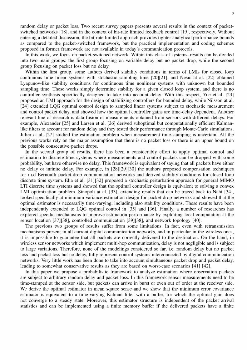
In this paper we propose a probabilistic framework to analyze estimation where observation packetsare subject to arbitrary random delay and packet loss. In this framework sensor measurements need to betime-stamped at the sensor side, but packets can arrive in burst or even out of order at the receiver side.We derive the optimal estimator in mean square sense and we show that the minimum error covarianceestimator is equivalent to a time-varying Kalman filter with a buffer, for which the optimal gain doesnot converge to a steady state. Moreover, this estimator structure is independent of the packet arrivalstatistics and can be implemented using a finite memory buffer if the delivered packets have a finite

4

maximum delay. In particular, the memory length is equal to the maximum packet delay of the receivedpackets. We also present two alternative estimator architectures which are computationally more efficient.In the first architecture, the estimator gains are constrained to be constant rather than stochastic as in thetime-varying optimal estimator. In the second architecture, smart sensors are used to preprocess data andimprove estimation performance. Also necessary and sufficient conditions for stability for these estimatorsare shown to depend only on the over packet loss probability and not on delay. We also provide numericalalgorithms to compute the expected error covariances of such estimators which turns out to be the solutionof modified algebraic Riccati equations and Lyapunov equations. These metrics can be used to comparedifferent communication protocols for real-time control applications as long as the packet arrival statisticsare known, i.i.d and stationary. Very importantly, these results do not depend on the specific implementationof the digital communication network (fieldbuses, Bluetooth, ZigBee, Wi-Fi, etc .. ) in the sense that it isnot necessary to modify the communication stack to implement the estimators.

III. PROBLEM FORMULATION

Consider the following discrete time linear stochastic plant:

xt+1 = Axt + wt (1)yt = Cxt + vt, (2)

where t ∈ N = {0, 1, 2, . . .}, x,w ∈ Rn, y ∈ Rm, A ∈ Rn×n, y ∈ Rm, C ∈ Rm×n, (x0, wt, vt) are Gaussian,uncorrelated, white, with mean (x0, 0, 0) and covariance (P0, Q, R) respectively. We also assume that thepair (A,C) is observable, (A,Q1/2) is reachable, and R > 01.

PLANT ESTIMATORDigital

Communication

Network

Digital

Communication

NetworkBuffer

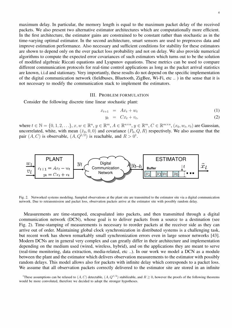
Fig. 2. Networked systems modeling. Sampled observations at the plant site are transmitted to the estimator site via a digital communicationnetwork. Due to retransmission and packet loss, observation packets arrive at the estimator site with possibly random delay.

Measurements are time-stamped, encapsulated into packets, and then transmitted through a digitalcommunication network (DCN), whose goal is to deliver packets from a source to a destination (seeFig. 2). Time-stamping of measurements is necessary to reorder packets at the receiver side as they canarrive out of order. Maintaining global clock synchronization in distributed systems is a challenging task,but recent work has shown remarkably small synchronization errors even in large sensor networks [43].Modern DCNs are in general very complex and can greatly differ in their architecture and implementationdepending on the medium used (wired, wireless, hybrid), and on the applications they are meant to serve(real-time monitoring, data extraction, media-related, etc ..). In our work we model a DCN as a modulebetween the plant and the estimator which delivers observation measurements to the estimator with possiblyrandom delays. This model allows also for packets with infinite delay which corresponds to a packet loss.We assume that all observation packets correctly delivered to the estimator site are stored in an infinite

1These assumptions can be relaxed to (A, C) detectable, (A, Q1/2) stabilizable, and R ≥ 0, however the proofs of the following theoremswould be more convoluted, therefore we decided to adopt the stronger hypotheses.

5

buffer, as shown in Fig. 2. The arrival process is modeled via the random variable γtk defined as follows:

γtk =

{1 if yk has arrived at the estimator before or at time t, t ≥ k0 otherwise (3)

From this definition it follows that (γtk = 1) ⇒ (γt+h

k = 1,∀h ∈ N), which simply states that if packet yk

is present in the receiver buffer at time t, then it will be present for all future times. We also define thepacket delay τk ∈ {N,∞} for observation yk as follows:

τk =

{ ∞ if γtk = 0,∀t ≥ k

tk − k otherwise, where tk∆= min{t | γt

k = 1} (4)

where tk is the arrival time of observation yk at the estimator site . Since the packet delay can be random,observation measurements can arrive out of order at the estimator site (see Fig. 3, t = 5). Also it ispossible that between two consecutive sampling periods no packet (see Fig. 3, t = 4) or multiple packets(see Fig. 3, t = 6) are delivered. In our work we do not consider quantization distortion due to dataencoding/decoding since we assume that observation noise is much larger then quantization noise, as itis the case in most DCNs where each packet allocates hundreds of bits for measurement data2. Also wedo not consider channel noise since we assume that if any bit error incurred during packet transmissionis detected at the receiver, then the packet is dropped.

Fig. 3. Packet arrival sequence and buffering at the estimator location. Shaded squares correspond to observation packets that have beensuccessfully received by the estimator. Cursor indicates current time.

If observation yk is not yet arrived at the estimator at time t, we assume that a zero3 is stored in the2For example, ATM communication protocols adopts packets with 384-bit data field, Ethernet IEEE 802.3 packets allows for at least 368

bits for data payload, Bluetooth for 499 bits [18] and IEEE 802.15.4 for up to 1000 bits. This assumption might not hold for multimediasignal like audio and video signals, which however are not in the scope of this work.

3In practice, any arbitrary value can be stored in the buffer slots corresponding to the packets which have not arrived, since as it will beshown later, the optimal estimator does not use those values as they do not convey any information about the state xt. Our choice of storinga zero simply reduces some mathematical burden.

6

k-slot of the buffer, as shown in Fig. 3. More formally, the value stored in the k-slot of the estimatorbuffer at time t can be written as follows:

ytk = γt

kyk = γtkCxk + γt

kvk (5)

Our goal to compute the optimal mean square estimator xt|t which is given by:

xt|t∆= E[xt | yt,γt, x0, P0] (6)

where yt = (yt1, y

t2, . . . , y

tt) and γt = (γt

1, γt2, . . . , γ

tt). It is important to remark that the estimator above

has the information whether a packet has been delivered or not, and it is not equivalent to computingxt|t 6= xt|t

∆= E[xt | yt, x0, P0]. The latter estimator would in fact consider the zero entries of the buffer

as true measurements and not as dummy variables, thus providing a lower performance. It is also usefulto design the estimator error and error covariance as follows:

et|t∆= xt − xt|t (7)

Pt|t∆= E[ et|te

Tt|t | yt,γt, x0, P0] (8)

The estimate xt|t is optimal in the sense that it minimizes the error covariance, i.e. given any estimatorxt|t = f(yt,γt), where f is a measurable function, we always have

E[(xt − xt|t)(xt − xt|t)T | yt,γt, x0, P0] ≥ Pt|t.

Another property of the mean square optimal estimator is that xt|t and its error et|t∆= xt − xt|t are

uncorrelated, i.e. E[et|t xTt|t] = 0. This is a fundamental property since it is necessary to give rise to the

separation principle for the LQG optimal control, which is one of the most widely used tool in controlsystem design [15] [36].

IV. MINIMUM ERROR COVARIANCE ESTIMATOR DESIGN

In this section we want to compute the optimal estimator given by Equation (6). First, it is convenientto define the following variables:

xtk|h

∆= E[xk | γt

h, . . . , γt1, y

th, . . . , y

t1, x0, P0]

P tk|h

∆= E[(xk − xt

k|h)(xt − xtk|h)

T | γth, . . . , γ

t1, y

th, . . . , y

t1, x0, P0]

from which it follows that, with a little abuse of notation, xt|t = xtt|t and Pt|t = P t

t|t.It is also useful to note that at time t the information available at the estimator site, given by Equation (5),

can be written as the output of the following system:

xk+1 = Axk + wk (9)yt

k+1 = Ctk+1xk+1 + vt

k+1, k = 0, . . . , t− 1 (10)

where the random variables vtk

∆= γt

kvk are uncorrelated, zero mean white noise with covariance Rtk =

E[vtk(v

tk)

T ] = γtkR, and Ct

k∆= γt

kC. For any fixed t this system can be seen as a linear time-varyingsystem with respect to time k, where the only time-varying elements are the observation matrix Ct

k andmeasurement noise covariance Rt

k.We can now state the main theorem of this section:Theorem 1: Let us consider the stochastic linear system given in Equations (1)-(2), where R > 0. Also

consider the arrival process defined by Equation (3), and the mean square estimator defined in Equation (6).Then we have:

7

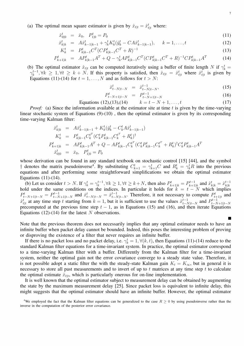
(a) The optimal mean square estimator is given by xt|t = xtt|t where:

xt0|0 = x0, P t

1|0 = P0 (11)

xtk|k = Axt

k−1|k−1 + γtkK

tk(y

tk − CAxt

k−1|k−1), k = 1, . . . , t (12)

Ktk = P t

k|k−1CT (CP t

k|k−1CT + R)−1 (13)

P tk+1|k = AP t

k|k−1AT + Q− γt

kAP tk|k−1C

T (CP tk|k−1C

T + R)−1CP tk|k−1A

T (14)

(b) The optimal estimator xt|t can be computed iteratively using a buffer of finite length N if γtk =

γt−1k , ∀k ≥ 1, ∀t ≥ k + N . If this property is satisfied, then xt|t = xt

t|t where xtt|t is given by

Equations (11)-(14) for t = 1, . . . , N and as follows for t > N :

xtt−N |t−N = xt−1

t−N |t−N , (15)

P tt−N+1|t−N = P t−1

t−N+1|t−N (16)Equations (12),(13),(14) k = t−N + 1, . . . , t (17)

Proof: (a) Since the information available at the estimator site at time t is given by the time-varyinglinear stochastic system of Equations (9)-(10) , then the optimal estimator is given by its correspondingtime-varying Kalman filter:

xtk|k = Axt

k−1|k−1 + Ktk(y

tk − Ct

kAxtk−1|k−1)

Ktk = P t

k|k−1CtT

k (CtkP

tk|k−1C

tT

k + Rtk)†

P tk+1|k = AP t

k|k−1AT + Q− AP t

k|k−1CtT

k (CtkP

tk|k−1C

tT

k + Rtk)†Ct

kPtk|k−1A

T

xt0|0 = x0, P t

1|0 = P0

whose derivation can be found in any standard textbook on stochastic control [15] [44], and the symbol† denotes the matrix pseudoinverse4. By substituting Ct

k+1 = γtk+1C and Rt

k = γtkR into the previous

equations and after performing some straightforward simplifications we obtain the optimal estimatorEquations (11)-(14).

(b) Let us consider t > N . If γtk = γt−1

k ,∀k ≥ 1,∀t ≥ k+N , then also P tk+1|k = P t−1

k+1|k and xtk|k = xt−1

k|khold under the same conditions on the indices. In particular it holds for k = t − N which impliesP t

t−N+1|t−N = P t−1t−N+1|t−N and xt

t−N |t−N = xt−1t−N |t−N . Therefore, it not necessary to compute P t

t+1|t andxt

t|t at any time step t starting from k = 1, but it is sufficient to use the values xt−1t−N |t−N and P t−1

t−N+1|t−N

precomputed at the previous time step t − 1, as in Equations (15) and (16), and then iterate EquationsEquations (12)-(14) for the latest N observations.

Note that the previous theorem does not necessarily implies that any optimal estimator needs to have aninfinite buffer when packet delay cannot be bounded. Indeed, this poses the interesting problem of provingor disproving the existence of a filter that never requires an infinite buffer.

If there is no packet loss and no packet delay, i.e. γtk = 1, ∀(k, t), then Equations (11)-(14) reduce to the

standard Kalman filter equations for a time-invariant system. In practice, the optimal estimator correspondto a time-varying Kalman filter with a buffer. Differently from the Kalman filter for a time-invariantsystem, neither the optimal gain not the error covariance converge to a steady state value. Therefore, itis not possible adopt a static filter the with the steady-state Kalman gain Kt = K∞, but in general it isnecessary to store all past measurements and to invert of up to t matrices at any time step t to calculatethe optimal estimate xt|t, which is particularly onerous for on-line implementation.

It is well known that the optimal estimator subject to measurement delay can be obtained by augmentingthe state by the maximum measurement delay [25]. Since packet loss is equivalent to infinite delay, thismight suggests that the optimal estimator should have an infinite buffer. However, the optimal estimator

4We employed the fact that the Kalman filter equations can be generalized to the case R ≥ 0 by using pseudoinverse rather than theinverse in the computation of the posterior error covariance.

8

can be implemented incrementally according to Equations (15)-(17) using a buffer of finite length Nif all successfully received observations have a delay smaller than N time steps, i.e. γt

k = γt−1k ,∀k ≥

1,∀t−k ≥ N (see Fig. 4). This does not mean that all packets arrive at the receiver within N time steps,but only that if a packet arrives then it does within N time steps.

ESTIMATOR

(A)ESTIMATOR

N

(B)

Fig. 4. Optimal estimator for general packet arrival processes (left). Optimal estimator with finite memory buffer for packet arrival processeswith bounded delay (right).

Up to this point we made no assumptions on the packet arrival process which can be deterministic,stochastic or time-varying. However, from an engineering perspective it is important to determine theperformance of the estimator, which is evaluated based on the error covariance Pt+1|t. If the packet arrivalprocess is stochastic, then also the error covariance is stochastic. In this scenario a common performancemetric is the expected error covariance, i.e. Eγ[Pt+1|t], where the expectation is performed with respectto the arrival process γt

k. However, other metrics can be considered, such as the probability that the errorcovariance exceeds a certain threshold, i.e. P[Pt+1|t > Pmax] [45]. In this work we focus on the expectederror covariance Eγ[Pt+1|t]. It is not clear whether is it possible to compute Eγ[Pt+1|t] analytically even fora simple Bernoulli arrival process, and so far only upper and lower bounds have been be obtained [33].Rather than trying to bound performance of the time-varying optimal estimator, in the next section we willfocus on filters with constant gains and with a finite buffer dimension, i.e. we will consider Kt

t−h = Kh forall t ∈ N, h = 0, . . . , N−1. The gains Kh will then be optimized to achieve the smallest error covariance atsteady-state. The advantage of using constant gains is that, differently from the optimal time-varying filter,it is not necessary to invert any matrix at all thus making it attractive for on-line applications. Moreover,since filters with constant gains are necessarily suboptimal, the computation of their error covarianceis useful per se as it provides an upper bound for the error covariance of the optimal minimum errorcovariance filter given by Equations (11)-(14).

V. OPTIMAL ESTIMATION WITH CONSTANT GAINS

In this section we will study minimum error covariance filters with constant gains under stationary i.i.darrival processes.Assumption: The packet arrival process at the estimator site is stationary and i.i.d. with the followingprobability function:

P[τt ≤ h] = λh (18)

where t ≥ 0, and 0 ≤ λh ≤ 1 is a non-decreasing in h = 0, 1, 2, . . ., and τt was defined in Equation (4).Equation (18) corresponds to the probability that a packet sampled h time steps ago has arrived at the

estimator. Obviously, λh must be non-increasing since λh = P[τt ≤ h−1]+P[τt = h] = λh−1 +P[τt = h].Also, we define the packet loss probability as follows:

λloss∆= 1− sup{λh| h ≥ 0} (19)

The arrival process defined by Equation (18) can be also be defined with respect to the probability densityof packet delay. In fact, by definition we have P[τk = 0] = λ0, P[τk = h] = λh − λh−1 for h ≥ 1, andP [τk = ∞] = λloss.

9

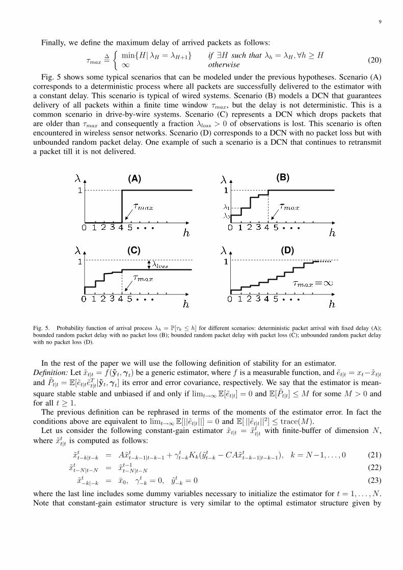
Finally, we define the maximum delay of arrived packets as follows:

τmax∆=

{min{H|λH = λH+1} if ∃H such that λh = λH , ∀h ≥ H∞ otherwise (20)

Fig. 5 shows some typical scenarios that can be modeled under the previous hypotheses. Scenario (A)corresponds to a deterministic process where all packets are successfully delivered to the estimator witha constant delay. This scenario is typical of wired systems. Scenario (B) models a DCN that guaranteesdelivery of all packets within a finite time window τmax, but the delay is not deterministic. This is acommon scenario in drive-by-wire systems. Scenario (C) represents a DCN which drops packets thatare older than τmax and consequently a fraction λloss > 0 of observations is lost. This scenario is oftenencountered in wireless sensor networks. Scenario (D) corresponds to a DCN with no packet loss but withunbounded random packet delay. One example of such a scenario is a DCN that continues to retransmita packet till it is not delivered.

(A) (B)

(C) (D)

Fig. 5. Probability function of arrival process λh = P[τk ≤ h] for different scenarios: deterministic packet arrival with fixed delay (A);bounded random packet delay with no packet loss (B); bounded random packet delay with packet loss (C); unbounded random packet delaywith no packet loss (D).

In the rest of the paper we will use the following definition of stability for an estimator.Definition: Let xt|t = f(yt,γt) be a generic estimator, where f is a measurable function, and et|t = xt−xt|tand Pt|t = E[et|teT

t|t|yt,γt] its error and error covariance, respectively. We say that the estimator is mean-square stable stable and unbiased if and only if limt→∞ E[et|t] = 0 and E[Pt|t] ≤ M for some M > 0 andfor all t ≥ 1.

The previous definition can be rephrased in terms of the moments of the estimator error. In fact theconditions above are equivalent to limt→∞ E[||et|t||] = 0 and E[ ||et|t||2] ≤ trace(M).

Let us consider the following constant-gain estimator xt|t = xtt|t with finite-buffer of dimension N ,

where xtt|t is computed as follows:

xtt−k|t−k = Axt

t−k−1|t−k−1 + γtt−kKk(y

tt−k − CAxt

t−k−1|t−k−1), k = N−1, . . . , 0 (21)

xtt−N |t−N = xt−1

t−N |t−N (22)

xt−k|−k = x0, γt

−k = 0, yt−k = 0 (23)

where the last line includes some dummy variables necessary to initialize the estimator for t = 1, . . . , N .Note that constant-gain estimator structure is very similar to the optimal estimator structure given by

10

Equation (12) as the estimate is corrected only if the observation has arrived, i.e. γtt−k = 1, otherwise

only the open loop prediction is considered. However, differently from Equation (12), the gains Kk, k =0, . . . , N−1 are constant and independent of t, and the computation of the estimate xt|t does not requireany on-line matrix inversion differently from the estimator in the previous section.

We also define the following variables that will be useful to analyze the performance of the estimator:

xtk+1|k = Axt

k|k (24)

etk+1|k = xk+1 − xt

k+1|k (25)

P tk+1|k = E[et

k+1|ketT

k+1|k | yt,γt] (26)

Pt

k+1|k = E[etk+1|ke

tT

k+1|k] = E[P tk+1|k] (27)

where t ≥ k ≥ 1. From these definitions we get:

etk+1|k = Axk + wk − A

(xk|k−1 + γt

kKt−k(γtkCxk + vk − Cxk|k−1)

)

= A(I − γtkKt−kC)et

k|k−1 + wk − γtkAKt−kvk (28)

P tk+1|k = A(I − γt

kKt−kC)P tk|k−1(I − γt

kKt−kC)T AT + Q + γtkAKt−kRKT

t−kAT (29)

Pt

k+1|k = λt−kA(I−Kt−kC)Pt

k|k−1(I−Kt−kC)TAT+(1−λt−k)APt

k|k−1AT+Q+λt−kA

TKt−kRKTt−kA

T(30)

where I ∈ Rn×n is the identity matrix. To obtain the previous equations we employed independence ofγt

k, vk, wk, and etk|k−1, and the fact that vk and wk are zero mean. For ease of notation let us define the

following operator:

Lλ(K, P ) = λA(I−KC)P (I−KC)T AT +(1−λ)APAT +Q+λAKRKT AT (31)

If we substitute k = t − N into Equation (30), and noting that from Equation (22) follows thatP t

t−N+1|t−N = P t−1t−N+1|t−N and P

t

t−N+1|t−N = Pt−1

t−N+1|t−N , we obtain:

Pt

t−N+2|t−N+1 = LλN−1(KN−1, P

t−1

t−N+1|t−N) (32)

Pt

t−k+1|t−k = Lλk(Kk, P

t

t−k|t−k−1), k = N−2, . . . , 0 (33)

Observe that Equations (32) and (33) define a set of linear deterministic equations for fixed λk and Kk.In particular, if we define St = P t−1

t−N+1|t−N , then Equations (32) can be written as

St+1 = LλN−1(KN−1, St) (34)

Since all matrices Pt

t−k+1|t−k, k = 0, . . . , N − 1 can be obtained from St it follows that stability ofestimator can be inferred from the properties of the operator Lλ(K,P ). The following lemma providesthese properties:

Lemma 1: Consider the operator Lλ(K, P ) as defined in Equation (31). Assume also that P ≥ 0,(A,C) is observable, (A,Q1/2) is reachable, R > 0, and 0 ≤ λ ≤ 1. Also consider the following operator:

Φλ(P ) = APAT + Q− λAPCT (CPCT + R)−1CPAT (35)

and the gain KP = PCT (CPCT + R)−1.Then the following statements are true:(a) Lλ(K,P ) = Φλ(P ) + λA(K −KP )(CPCT + R)(K −KP )T AT .(b) Lλ(K,P ) ≥ Φλ(P ) = Lλ(KP , P ), ∀K(c) (P1 ≥ P2) =⇒ (

Φλ(P1) ≥ Φλ(P2)).

(d) (λ1 ≥ λ2) =⇒ (Φλ1(P ) ≤ Φλ2(P )

), ∀P .

(e) If there exists P ∗ such that P ∗ = Lλ(K, P ∗), then P ∗ > 0 and it is unique. Consequently this istrue also for K = KP ∗ , where P ∗ = Φλ(P

∗).(f) If (λ1 ≥ λ2) and there exist P ∗

1 , P ∗2 such that P ∗

1 = Φλ1(P∗1 ) and P ∗

2 = Φλ2(P∗2 ), then P ∗

1 ≤ P ∗2 .

11

(g) Let St+1 = Lλ(K, St) and S0 ≥ 0. If S∗ = Lλ(K,S∗) has a solution, then limt→∞ St = S∗,otherwise the sequence St is unbounded.

(h) If there exists S∗, K such that S∗ = Lλ(K,S∗), then also P ∗ = Φλ(P∗) exists and P ∗ ≤ S∗.

(i) If A is strictly stable, then P ∗ = Φλ(P∗) has always a solution. Otherwise, there exist λc such that

P ∗ = Φλ(P∗) has a solution if and only if λ > λc. Also λmin ≤ λc ≤ λmax, where λmax = 1− 1∏

i |σui |2 ,

λmin = 1 − 1maxi |σu

i |2 , and |σui | ≥ 1 are the unstable eigenvalues of A. In particular λc = λmax if

rank(C) = 1, and λc = λmin if C is square and invertible.(j) The critical probability λc and the fixed point P ∗ = Φλ(P

∗) for λ > λc can be obtained as thesolutions of the following semi-definite programming (SDP) problems: λc = inf{λ |Ψλ(Y, Z) >0, 0 ≤ Y ≤ I, for some Z, Y ∈ Rn×n}, and P ∗ = argmax{trace(P ) |Θλ(P ) ≥ 0, P ≥ 0} where:

Ψλ(Y, Z) =

Y Y√

λZR12

√λ(Y A + ZC)

√1− λY A

Y Q† 0 0 0√λR

12 Z ′ 0 I 0 0√

λ(A′Y + C ′Z ′) 0 0 Y 0√1− λA′Y 0 0 0 Y

(36)

Θλ(P ) =

[APA′ − P

√λAPC ′√

λCPA′ CPC ′ + R

](37)

(k) If there exist P ∗ > 0 and K such that P ∗ = Lλ(K, P ∗), then the matrix Ac = A(I − λKC) isstrictly stable.Proof: See Appendix.

The previous lemma provides all tools necessary to analyze and design the optimal estimator withconstant gains. In particular, fact (g) indicates that the constant gain K∗ that minimizes the steady stateerror covariance P ∗ can be derived from the unique fixed point of the nonlinear operator P ∗ = Φλ(P

∗),where K∗ = KP ∗ . If the optimal gain K∗ is used, then the expected error covariance converges to P ∗

regardless of the initial conditions (P0, x0), as follows from fact (f). Fact (i) shows that if the system Ais unstable the arrival probability λ needs to be sufficiently large to ensure stability, and that the criticalvalue λc is a function of the unstable eigenvalues of A. Finally, although λc and the the fixed pointP ∗ = Φλ(P

∗) cannot be computed in closed form, from fact (j) follows that they can be efficientlycomputed using numerical optimization tools. Finally, fact (k) will be used to show that if the errorcovariance is bounded then the estimator is also unbiased.

The following theorem shows how compute the optimal estimator with constant gains.Theorem 2: Let us consider the stochastic linear system given in Equations (1)-(2), where (A,C) is

observable, (A,Q1/2) is reachable, and R > 0. Also consider the arrival process defined by Equations (18)-(20), and the set of estimators with constant gains {Kk}N

k=0 defined in Equations (21)-(23). If A is notstrictly stable and λloss ≥ 1− λc, where λc is defined in Lemma 1(j), then there exist no stable estimatorwith constant gains. Otherwise, let N such that λN > λc and consider the optimal gains {KN

k }Nk=0 defined

as follows:

KNk = V N

k CT (CV Nk CT + R)−1, k = 0, . . . , N (38)

V NN−1 = ΦλN−1

(V NN−1) (39)

V Nk = Φλk

(V Nk+1), k = N − 1, . . . , 0 (40)

Also consider Pt

k+1|k as defined in Equation (27), then limt→∞ Pt

t−k+1|t−k = V Nk , independently of initial

conditions (P0, x0). For any other choice of gains {Kk}Nk=0 for which the solution {Tk}N

k=0 to the followingequations exist:

TNN = LλN

(KN , TNN ) (41)

TNk = Lλk

(Kk, TNk+1), k = N − 1, . . . , 0 (42)

12

then limt→∞ Pt

t−k+1|t−k = TNk , and V N

k ≤ TNk for k = 0, . . . , N . Also V N+1

0 ≤ V N0 . Finally, if τmax < ∞,

then V N0 = V τmax

0 for all N ≥ τmax.Proof: See Appendix.

The previous theorem shows that the optimal gains can be obtained by finding the fixed point of amodified algebraic Ricatti Equation (39) and then iterating N time an operator with the same structurebut with different λk. The theorem also demonstrates that a stable estimator with constant gains exists if andonly if the optimal estimator with constant gains exists, therefore the optimal estimator design implicitlysolves the problem of existence of stable estimators. If the system to be estimated is unstable, then theestimator is stable if and only if the packet loss probability λloss is sufficiently small, independentlyof the packet delay τmax, thus recovering the same stability conditions derived in [33]. Moreover, theperformance of the estimator, i.e. its steady state error covariance limt→∞ Pt+1|t = limt→∞ E[et+1|teT

t+1|t] =

V N0 , improves as the buffer length N is increased, which is to be expected since more information is

stored. However, if the maximum packet delay is finite τmax < ∞, then the performance of the estimatordoes not improve for N > τmax. This is consistent with Theorem 1(b) since if a measurement packet hasnot arrived within τmax time steps after it was sampled, then it will never arrive and it is useless to waitlonger.

From a practical perspective, the previous tools can be used by the designer to evaluate the tradeoffbetween the estimator performance V N

0 and buffer length N which is directly related to computationalrequirements.

VI. OPTIMAL ESTIMATION WITH CO-LOCATED SMART SENSORS

In this section we describe an alternative data pre-processing at the sensor location which improvesthe overall performance of the estimator at the receiver side. This scheme was independently proposedin [46] and [37] in a scenario where no delay was present but only packet loss. The authors suggestedto compute and transmit the state estimate rather than the raw measurement. As will be shown shortly,this approach gives an estimator that has a better performance as compared to the time-varying Kalmanfilter of Section IV. However, it is applicable only if some computational resources are available on thesensor, commonly known as “smart sensor”, and if all entries of the observation vector yt are collectedfrom sensors which are co-located. For example, this scenario is not suitable in applications running oversensor networks where sensors are distributed and have very limited computation resources [47]. Addingspecific coding schemes and data processing at the sensor side could further improve performance, butthis would require the modification of the lower layers of the communication protocols, differently fromthe architecture proposed here. Besides, this estimator architecture proposed here is useful per se sinceit provides a computable lower bound for the performance of the optimal time-varying filter proposed inSection IV.

PLANT+SENSOR

DECODER

ESTIMATORDigitalCommunication

Network

DigitalCommunication

Network

ENCODERESTIMATOR

Fig. 6. Smart sensor with state estimator at encoder site before transmission.

Rather than sensing the raw measurements yt over the DCN the sensor compute the optimal state

13

estimate as follows:

xet = Axe

t−1 + Ket (yt − Axe

t−1) (43)Ke

t = P et CT (CP e

t CT + R)−1 (44)P e

t+1 = AP et AT + Q− AP e

t CT (CP et CT + R)−1CP e

t AT = Φ1(Pt) (45)P e

0 = P0, xe0 = x0 (46)

These are the equations for the standard Kalman filter, i.e. the minimum error covariance estimator xet =

E[xt | yt, . . . , y1] whose estimation error eet = xt+1−Axe

t has covariance cov(eet) = E[ee

teeT

t | yt, . . . , y1] =P e

t . The state estimate computed by the sensor encoder is then transmitted over the DCN to the decoderestimator. Using the same notation of Equation (5) the value stored at the buffer can be written as follows:

ytk = γt

kxek (47)

Let us define the delay of the most recent packet arrived at the decoder estimator as κt = t−max{k | γtk = 1}

if ∃γtk = 1, or κt = t otherwise. The estimate of current state at the decoder estimator xd

t is computed asfollows:

xdt = Aκt yt

t−κt= Aκt xe

t−κt(48)

Note that the decoder estimate is equivalent to xdt = E[xt | yt−κt , . . . , y1] and that the its error ed

t = xt+1 − Axdt

has covariance:

cov(edt ) = E[ed

t edT

t | yt−κt , . . . , y1] = Φt−κt0 (E[ed

t−κtedT

t−κt| yt−κt , . . . , y1]) = Φt−κt

0 (P et−κt

) = Φt−κt0 ◦Φκt

1 (P0),

where the superscript of Φnλ(P ) indicates Φλ ◦ · · · ◦ Φλ(P ) composed n-times. Therefore, the decoder

estimator error at any time step t is equivalent to the optimal estimator that one would obtain if allobservations up to time t− κt were successfully delivered. This estimation architecture is superior to theestimation architecture proposed in Section IV, in fact the estimator obtained in Theorem 1 has errorcovariance cov(xt+1 − Axt

t|t) = P tt+1|t, where P t

t+1|t is given by Equations (13)-(14) and can be writtenas:

P tt+1|t = Φγt

t◦ . . . ◦ Φγt

1(P0)

= Φt−κt0 ◦ Φγt

κt◦ . . . ◦ Φγt

1(P0)

≥ Φt−κt0 ◦ Φγt

κt◦ . . . ◦ Φ1(P0)

≥ Φt−κt0 ◦ Φ1 ◦ . . . ◦ Φ1(P0)

= Φt−κt0 ◦ Φκt

1 (P0)

= cov(edt )

where we used the facts γtk = 0 for k > κt, γt

k ≤ 1 for k ≤ κt, and Lemma 1(d). Therefore, the errorcovariance of the estimator proposed in this section is smaller than the error covariance of estimatorproposed in Section IV. We can summarize the previous result in the following theorem:

Theorem 3: Let us consider the stochastic linear system given in Equations (1)-(2), where R > 0. Alsoconsider the packet arrival process defined by Equation (3). Let xy

t = xtt|t the optimal estimator given by

Equations (11)-(14) when raw measurements yt are transmitted over the network. Let xdt the estimator

given by Equation (48) where the state estimate xet defined by Equations (43)-(46) is pre-computed by

the sensor and then transmitted over the network. Then the estimation error covariance of xet is always

smaller than the estimation error covariance of xtt, i.e.

cov(xt − xdt ) ≤ cov(xt − xy

t ), ∀t.Besides having a better performance, the estimator proposed in this section requires very limited

computational requirements at the receiver side, in fact it suffices to store the most recent packet arrived

14

at the receiver and then to compute the best state estimate at current time by pre-multiplying the packetdata with a matrix which depend on the packet delay. Moreover, as for the estimator of Section IV, alsothe estimator based on co-located smart sensors does not require any statistical a-priori knowledge of thearrival process.

However, if the packet arrival statistics are stationary and i.i.d, then it is possible to give stability criteriaand to compute the expected error covariance as shown in the following theorem:

Theorem 4: Let us consider the stochastic linear system given in Equations (1)-(2), where (A,C) isobservable, (A,Q1/2) is reachable, and R > 0. Also consider the arrival process defined by Equations (18)-(20), and the estimator architecture given by Equations (43)-(48). Then the estimator is stable if and only ifA is stable, or λloss < 1

|σumax(A)|2 , where σu

max(A) is the largest eigenvalue of the matrix A. If the estimatoris stable then the covariance of the estimation error defined as ed

t = xt+1−Axdt has the following property:

limt→∞

E[edt e

dT

t ] = D∞ = limN→∞

DN0 (49)

where the matrix DN0 is computed as follows:

DNN = (1− λN)ADN

N AT + (1− λN)Q + λNP e∞ (50)

DNk = (1− λk)ADN

k+1AT + (1− λk)Q + λkP

e∞, k = N − 1, . . . , 0 (51)

and P e∞ is the unique positive definite solution of the Ricatti Equation P e

∞ = Φ1(Pe∞). If τmax < ∞, then

D∞ = Dτmax0 = DN

0 , for all N ≥ τmax.Proof: See Appendix.

The previous theorem shows that performance of the smart optimal estimator under the assumption ofi.i.d. packet arrival process, can be obtained by solving the Lyapunov Equation (50) and then iteratingN = τmax linear equations (51), if τmax is finite. Otherwise if τmax = ∞, then D∞ can be computed toany arbitrary precision through the sequence DN

0 .

VII. NUMERICAL EXAMPLES

Here we illustrate the use of the tools developed in the previous sections with the aid of some numericalexamples.

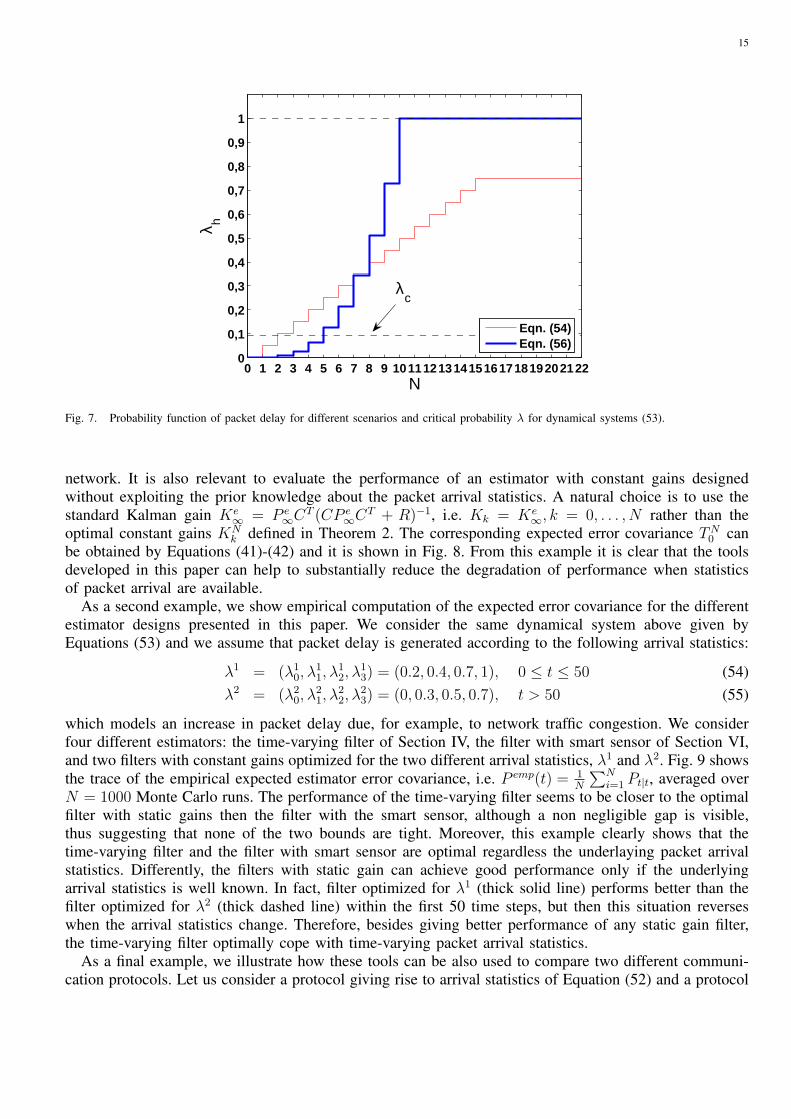
Let us consider the following probability function of packet delay:

λh =

{0.05 h, h = 0, . . . , 150.75, h > 15

(52)

which is depicted in Fig. 7.Let us consider the following discrete time system:

A =

[1.001 0.050.05 1.001

], C = [ 1 0 ], R = 0.01, Q =

[0 00 0.01

](53)

which corresponds to the discretization with sampling period T = 0.05 of the continuous time sys-tem x − x = 0. This system has one stable pole and one unstable pole, and it is the model forthe discrete time dynamics of an inverted pendulum. The discrete time eigenvalues of the matrix Aare eig(A) = (1.05, 0.95), which give the critical probability λc = 1 − 1/1.052 = 0.095, as statedin Lemma 1(i). According to Theorem 2 and Theorem 4 both estimators presented in Section V andSection VI are stable if and only if N ≥ 2, in fact λ1 = 0.05 < λc and λ2 = 0.01 > λc.

The trace of the covariance of the estimator error with constant gains, V N0 , and the estimator error for

smart sensors, DN0 are shown in Fig. 8. As mentioned in Section IV, the error covariance for time-varying

optimal estimator of Theorem 1 cannot be computed explicitly but it is upperbounded and lowerboundedby V N

0 and by DN0 , respectively. It is interesting to compare the performance of these estimators with the

error covariance P e∞ = Φ1(P

e∞), shown in the same figure, corresponding to the ideal case when there

is no packet loss and no delay. In fact, P e∞ gives an idea of the degradation due to the communication

15

0 1 2 3 4 5 6 7 8 9 101112131415161718192021220

0,1

0,2

0,3

0,4

0,5

0,6

0,7

0,8

0,9

1

N

λ h

Eqn. (54)Eqn. (56)

λc

Fig. 7. Probability function of packet delay for different scenarios and critical probability λ for dynamical systems (53).

network. It is also relevant to evaluate the performance of an estimator with constant gains designedwithout exploiting the prior knowledge about the packet arrival statistics. A natural choice is to use thestandard Kalman gain Ke

∞ = P e∞CT (CP e

∞CT + R)−1, i.e. Kk = Ke∞, k = 0, . . . , N rather than the

optimal constant gains KNk defined in Theorem 2. The corresponding expected error covariance TN

0 canbe obtained by Equations (41)-(42) and it is shown in Fig. 8. From this example it is clear that the toolsdeveloped in this paper can help to substantially reduce the degradation of performance when statisticsof packet arrival are available.

As a second example, we show empirical computation of the expected error covariance for the differentestimator designs presented in this paper. We consider the same dynamical system above given byEquations (53) and we assume that packet delay is generated according to the following arrival statistics:

λ1 = (λ10, λ

11, λ

12, λ

13) = (0.2, 0.4, 0.7, 1), 0 ≤ t ≤ 50 (54)

λ2 = (λ20, λ

21, λ

22, λ

23) = (0, 0.3, 0.5, 0.7), t > 50 (55)

which models an increase in packet delay due, for example, to network traffic congestion. We considerfour different estimators: the time-varying filter of Section IV, the filter with smart sensor of Section VI,and two filters with constant gains optimized for the two different arrival statistics, λ1 and λ2. Fig. 9 showsthe trace of the empirical expected estimator error covariance, i.e. P emp(t) = 1

N

∑Ni=1 Pt|t, averaged over

N = 1000 Monte Carlo runs. The performance of the time-varying filter seems to be closer to the optimalfilter with static gains then the filter with the smart sensor, although a non negligible gap is visible,thus suggesting that none of the two bounds are tight. Moreover, this example clearly shows that thetime-varying filter and the filter with smart sensor are optimal regardless the underlaying packet arrivalstatistics. Differently, the filters with static gain can achieve good performance only if the underlyingarrival statistics is well known. In fact, filter optimized for λ1 (thick solid line) performs better than thefilter optimized for λ2 (thick dashed line) within the first 50 time steps, but then this situation reverseswhen the arrival statistics change. Therefore, besides giving better performance of any static gain filter,the time-varying filter optimally cope with time-varying packet arrival statistics.

As a final example, we illustrate how these tools can be also used to compare two different communi-cation protocols. Let us consider a protocol giving rise to arrival statistics of Equation (52) and a protocol

16

0 1 2 3 4 5 6 7 8 9 101112131415161718192021220

0.1

0.2

0.3

0.4

0.5

0.6

0.7

0.8

0.9

1

N

trac

e(P

N)

V0N

D0N

T0N

P∞e

Fig. 8. Trace of the steady state error covariance for the optimal estimator with constant gains (V N0 ), for the optimal estimator with a smart

sensor (DN0 ). The horizontal line P e

∞ corresponds to the trace of the error covariance in the ideal scenario with no delay and no packetloss, i.e. λh = 1 for all h, while T N

0 is the actual steady state error when using the Kalman gain Ke∞. The error covariances V N

0 , DN0 are

unbounded for N < 2, while the covariance P e∞ is unbounded for N < 4, and they are all cosnstant constant for N ≥ τmax = 15.

giving rise to the following arrival statistics:

λh =

{( h

10)3, h = 0, . . . , 10

1, h > 10(56)

for which τmax = 10, and it is graphically shown in Fig. 7. These two protocols are substantially different:the first protocol has larger packet delivery with small delay, but also larger overall packet loss than the firstprotocol, therefore it is difficult to evaluate which one is better suited for a real-time control application.In Fig. 10 it is shown the trace of the error covariance V N

0 for the two protocols with respect to thesystem dynamics of Equation (53). For a buffer with a short memory the first protocol performs better,but for a buffer of length N = 10 the second protocol starts performing better as the larger packet deliverycan compensate for a larger delay of arrived packets. If buffer length is further increased, then the firstprotocol returns to perform better. This example clearly shows how optimal estimation design can be usedto evaluate and compare the performance of different communication protocols with respect to a specificreal-time application, which is otherwise very difficult if based on intuition or empirical rule-of-thumbs.

VIII. CONCLUSIONS

In this work we proposed a framework to optimally design and analyze the performance of estimatorsin networked control system subject to simultaneous random packet delay and packet dropped. We showedthat the optimal estimator is time-varying, stochastic, and does not depend on the specific communicationprotocol adopted as long as measurements are time-stamped and can be re-ordered at the estimator site.Also two alternative optimal estimator designs based on finite memory buffers and constant gains weredescribed and it was shown that if packet arrival is i.i.d., then the estimators are mean square stable ifand only if the packet loss probability is below a critical value. Therefore, implicitly we also providednecessary and sufficient conditions about existence of stable estimators. Finally, we presented numericalalgorithms for the computation of the expected estimator error covariance of all the proposed estimators.

17

0 10 20 30 40 50 60 70 80 90 1000.9

1

1.1

1.2

1.3

1.4

1.5

1.6

1.7

1.8

time (t)

Tra

ce(

E[P

t|t] )

Time−varying gainSmart SensorStatic gain, λ1

Static gain, λ2

Fig. 9. Time series of trace of trace of empirical error covariance P emp(t) ∼= E[Pt|t] averaged over 1000 Monte Carlo runs for fourdifferent estimators under the same conditions. The packet delay arrival probability distribution changes from λ1 to λ2 at time t = 50. Thefilters with static gains are optimized for λ1 and λ2.

The tools developed in this paper are useful both from a control system design perspective and froma communication design perspective. In fact, from a control perspective they can help to evaluate thetradeoffs between performance (error covariance), memory requirements (buffer length), and the hardwareresources (“smart” sensor and fast matrix inversion). In particular, the knowledge of the packet arrivalstatistics can be used to find the optimal constant gains {KN

k }Nk=0 and thus improving performance. From

a communication perspective, these tools can be used to aid communication protocol design for real-timeapplications. In fact, as mentioned in Section I, when designing communication protocols, in particular forwireless systems, there is tradeoff between packet loss and packet delay. At the moment, the choice betweenfavoring reduction of overall packet delay or reduction of packet loss is based on heuristics and experience,and it is not tailored to the specific real-time applications. Therefore, being able to quantitatively measureperformance of different protocols can improve cross-layer design of complex networked control systems.

A possible future avenue of research is the extension of this work to the design of optimal LQG-likecontroller design. This is not a trivial step as many important assumptions in standard LQG control, like theseparation principle, do not always hold for NCSs [36]. Another research direction is the implementationand testing of these tools in real-time control applications for wireless sensor networks. A preliminaryattempt has already been successfully applied to multiple target tracking [48], but extensive experimentalwork is still needed.

IX. APPENDIX

Proof of Lemma 1. Some of these statements can be found in [33] or can be derived along similar lines,therefore only a brief sketch is reported here.

(a) This fact can be verified by direct substitution(b) This statement follows from previous fact and λA(K −KP )(CPCT + R)(K −KP )T AT ≥ 0.(c) From previous fact Φλ(P1) = Lλ(KP1 , P1) ≥ Lλ(KP1 , P2) ≥ Lλ(KP2 , P2) = Φλ(P2).(d) From Equation (35) we have Φλ1(P )− Φλ2(P ) = −(λ1 − λ2)APCT (CPCT + R)−1CPAT ≤ 0.(e) Uniqueness and strictly positive definiteness of P ∗ follows from the assumption that (A, Q1/2) is

reachable [33].

18

0 1 2 3 4 5 6 7 8 9 101112131415161718192021220.3

0.35

0.4

0.45

0.5

0.55

0.6

N

trac

e(V

0N)

Eqn. (54)Eqn. (56)

Fig. 10. Trace of the steady state error covariance for the optimal estimator with constant gains (V N0 ) for two different communication

protocols whose packet arrival statistics is given by Equations (52) and (56).

(f) Consider Pt+1 = Φλ1(Pt) and St+1 = Φλ2(St) where P0 = S0 = 0. From fact (c) and (e) it followsthat Pt ≤ St. Also Pt ≤ P ∗

1 and St ≤ P ∗2 , therefore limt→∞ Pt = P , limt→∞ St = S, and P ≤ S. From

fact (e) it follows that P = P ∗1 and S = P ∗

2 , and thus P ∗1 ≤ P ∗

2

(g-h) Let consider Pt+1 = Φλ(Pt) and St+1 = Lλ(K, St) where P0 = S0 = 0. From fact (c) andmonotonicity of operator Lλ(K,P ) with respect to P we have Pt+1 ≥ Pt, St+1 ≥ St, and Pt ≤ St ≤S∗ for all t. Since both sequences are monotonically increasing and bounded, then limt→∞ Pt = P ,limt→∞ St = S, P = Φλ(P ), S = Lλ(K, S), and P ≤ S. From fact (e) it follows that P = P ∗ andS = S∗. A complete proof for convergence from any initial condition can be obtained along the lines ofTheorem 1 in [33], thus it is not reported here.

(i) The proof for existence of a critical probability λc was given in [33] and it is based on observabilityof (A,C) and monotonicity of Φλ(P ) with respect to λ. The proof for λc = λmax when rank(C) = 1 canbe found in [49][32] although it was not explicitly derived for the operator Φλ. The proof for λc = λmin

when C is square and invertible was first proved in [50].(j) The proof can be found in [33].(k) Let us consider the linear operator F(P ) = λA(I−KC)P (I−KC)T AT +(1−λ)APAT . Clearly

Lλ(K,P ) = F(P ) + D, where D = Q+λAKRKT AT ≥ 0. Consider the sequences St+1 = Lλ(KP ∗ , St),Tt+1 = Lλ(KP ∗ , Tt) with initial condition S0 = 0, then T0 ≥ 0. Note that St =

∑t−1k=0Fk(D) and

Tt = F t(T0)+∑t−1

k=0Fk(D) for t ≥ 1, where we define F0(D) = D and Fk+1(D) = F◦Fk(D). ThereforeF t(T0) = Tt − St. From fact (g) it follows limt→∞ St = limt→∞ Tt = P ∗, therefore limt→∞F t(T0) = 0,for all T0 ≥ 0, i.e. the linear operator F() is strictly stable. Now consider the system Ac = A(I −λKC). The system is strictly stable if and only if limt→∞ At

cx0 = 0, for all x0. This is equivalent tolimt→∞ At

cx0xT0 (AT

c )t = Gt(X0) = 0, where X0 = x0xT0 ≥ 0 and Gt(X0) = At

cX0(ATc )t. Note that

G(X0) = AX0AT − 2λAX0(AKC)T + λ2AKCX0(AKC)T = F(X0) + λ(λ − 1)AKCX0(AKC)T ≤

F(X0) since λ(λ−1)AKCX0(AKC)T ≤ 0. Since we just proved that limt→∞F t(X0) = 0 for all X0 ≥ 0,then also limt→∞ Gt(X0) ≤ F t(X0) = 0 for X0 = x0x

T0 , i.e. the system Ac is strictly stable. ¥

Proof of Theorem 2. First we prove by contradiction that there is no stable estimator with constant gains ifA is not strictly stable and λloss ≥ 1−λc. Suppose such an estimator exists, i.e. there exist N and {Kk}N−1

k=0

19

such that Pt

t|t is bounded for all t. Since Pt

t+1|t = APt

t|tAT +Q also P

t

t+1|t must be bounded for all t. FromEquations (32) and (33) it follows that P

t

t+1|t is bounded if and only if Pt

t−k+1|t−k for k = 0, . . . , N−1 arebounded for all t. Therefore, since the bounded sequence St = P

t

t−N+1|t−N needs to satisfy Equation (34),from Lemma 1(g) follows that S∗ = LλN−1

(KN−1, S∗) has a solution. From Lemma 1(h) follows that

also P ∗ = ΦλN−1(P ∗) has a solution. However, by hypothesis λN−1 ≤ sup{λh |h ≥ 0} = 1− λloss ≤ λc.

Consequently, according to Lemma 1(i), P ∗ = ΦλN−1(P ∗) cannot have a solution, which contradicts the

hypothesis that a stable estimator exists.Consider now the case when N is such that λN > λc. From Theorem 1(h) it follows that Equations (38)-

(40) are well defined and have a solution. From Lemma 1(g) it follows that limt→∞ Pt

t−k+1|t−k = V Nk

for the optimal gains {KNk }N−1

k=0 , and limt→∞ Pt

t−k+1|t−k = TNk when using generic gains {Kk}N−1

k=0 .From Lemma 1(h) it follows that V N

N−1 ≤ TNN−1. From Lemma 1(c) we have V N

N−2 = ΦλN−2(V N

N−1) ≤LλN−2

(KN−2, VNN−1) ≤ LλN−2

(KN−2, TNN−1) = TN

N−2. Inductively, it is easy to show that V Nk ≤ TN

k forall k = 0, . . . , N − 1.

Now we want to show that V N+10 ≤ V N

0 . From Lemma 1(f) and the property λN+1 ≥ λN follow alsothat V N+1

N+1 = ΦλN+1(V N+1

N+1 ) ≤ V NN = ΦλN

(V NN ). Therefore V N+1

N = ΦλN(V N+1

N+1 ) ≤ ΦλN(V N

N ) = V NN and

inductively V N+1k ≤ V N

k for all k = N, . . . , 0 which proves the statement.Finally, if τmax is finite, then λk = λτmax for all k ≥ τmax. Assume N > τmax, then V N

N = ΦλN(V N

N ) =ΦλN−1

(V NN ) = V N

N−1 = ΦλN−1(V N

N−1) = ΦλN−2(V N

N−1) = V NN−2 = . . . = V N

τmax= Φλτmax

(V Nτmax

). SinceV τmax

τmax= Φλτmax

(V τmaxτmax

), then by Lemma 1(e) we have that V τmaxτmax

= V Nτmax

. According to Equation (40)we also have V τmax

k = V Nk for k = τmax, . . . , 0, which concludes the theorem. ¥

Proof of Theorem 4. The proof follows along the same lines of Theorems 1 and 2. Let us consider thefollowing estimator:

xtt−N |t−N = (1− γt

t−N)Axt−1t−N−1|t−N−1 + γt

t−N xst−N

xtt−k|t−k = (1− γt

t−k)Axtt−k−1|t−k−1 + γt

t−kxst−k, k = N−1, . . . , 0

xt−k|−k = x0, γt

−k = 0, xs−k = 0

It should be clear that by construction xdt = xt

t|t if and only if N ≥ τmax. If N < τmax, then the estimatorxd

t cannot be optimal. Let us consider the estimator error defined as etk+1|k = xk+1 − Axt

k|k that can bewritten as:

etk+1|k = xk+1 − A

((1− γt

k)Axtk−1|k−1 + γt

kxsk

)= (1− γt

k)(xk+1 − AAxt−1k−1|k−1) + γt

k(xk+1 − Axsk)

= (1− γtk)(A(xk − Axt−1

k−1|k−1) + wk) + γtke

sk = (1− γt

k)(Aetk|k−1 + wk) + γt

kesk

and its error covariance P tk+1|k = E[et

k+1|ketT

k+1|k | γtk, . . . , γ

t1] is then given by:

P tt−N+1|t−N = (1− γt

t−N)(AP t−1t−N |t−N−1A

T + Q) + γtt−NP e

t−N

P tt−k+1|t−k = (1− γt

t−k)(AP tt−k|t−k−1A

T + Q) + γtt−kP

et−k, k = N−1, . . . , 0

P t−k|−k = P0, γt

−k = 0

The error covariance P tt+1|t is then stochastic and depends on the arrival sequence. However since it is

linear in the arrival sequence γtk, it is possible to compute the expected error covariance E[P t

k+1|k] = P tk+1|k

as follows:

P tt−N+1|t−N = (1− λN)AP t−1

t−N |t−N−1AT + (1− λN)Q + λNP s

t−N

P tt−k+1|t−k = (1− λk)AP t

t−k|t−k−1AT + (1− λk)Q + λkP

st−k, k = N−1, . . . , 0

P t−k|−k = P0, γt

−k = 0

20

Since limt→∞ P et−k = P e

∞ where P e∞ = Φ1(P

e∞), then limt→∞ P t

t−N+1|t−N = DNN exists and it is finite if

and only if√

1− λNA is stable, i.e.√

1− λN |σumax(A)| < 1. This is equivalent to λN > 1 − 1

|σumax(A)|2 .

Such λN exists if and only if λloss < 1|σu

max(A)|2 . If this condition holds then Equations (50)-(51) follow.Also it is simple to show that {DN

0 }∞N=0 is a decreasing function of N and bounded from below,therefore limN→∞ DN

0 = D∞. Moreover, since by construction limN→∞ xdt = xt

t|t, then also E[edt e

dT

t ] =

limN→∞ P tt+1|t, and therefore it follows limt→∞ E[ed

t edT

t ] = D∞. Following Theorem 2, it is easy to showthat if τmax < ∞, then D∞ = Dτmax

0 = DN0 , for all N ≥ τmax, which concludes the theorem. ¥

REFERENCES

[1] “Technology of networked control systems,” Proceedings of the IEEE, Special issue, vol. 95, no. 1, pp. 5–312, January 2007.[2] M. Kintner-Meyer and R. Conant, “Opportunities of wireless sensors and controls for building operation,” Energy Engineering Journal,

vol. 102, no. 5, pp. 27–48, 2005.[3] M. Nekovee, “Ad hoc sensor networks on the road: the promises and challenges of vehicular ad hoc networks,” in Workshop on

Ubiquitous Computing and e-Research, Edinburgh, UK, May 2005.[4] S. Oh, L. Schenato, P. Chen, and S. Sastry, “Tracking and coordination of multiple agents using sensor networks: system design,

algorithms and experiments,” To appear in Proceedings of IEEE.[5] R. Szewczyk, E. Osterweil, J. Polastre, M. Hamilton, A. M. Mainwaring, and D. Estrin, “Habitat monitoring with sensor networks,”

Communication of the ACM, vol. 47, no. 6, pp. 34–40, 2004.[6] G. Tolle, J. Polastre, R. Szewczyk, N. Turner, K. Tu, P. Buonadonna, S. Burgess, D. Gay, W. Hong, T. Dawson, and D. Culler, “A

macroscope in the redwoods,” in Proceedings of the Third ACM Conference on Embedded Networked Sensor Systems (SenSys05), SanDiego, CA, USA, November 2005, pp. 51–63.

[7] A. Willig, K. Matheus, and A.Wolisz, “Wireless technology in industrial networks,” Proceedings of the IEEE, vol. 93, no. 6, pp.1130–1151, June 2005.

[8] “Sensor networks and applications,” Proceedings of the IEEE, Special issue, vol. 91, August 2003.[9] R. Ahlswede, N. Cai, S.-Y. R. Li, and R. W. Yeung, “Network information flow,” IEEE Transactions on Information Theory, vol. 46,

pp. 1204–1216, 2000.[10] R. Cristescu and M. Vetterli, “On the optimal density for real-time data gathering of spatio-temporal processes in sensor networks,” in

Proceedings of the Fourth International Symposium on Information Processing in Sensor Networks, IPSN05, 2005, pp. 159–164.[11] H. Durrant-Whyte, M. Stevens, and E. Nettleton, “Data fusion in decentralised sensing networks,” in Proceeding on Information Fusion

2001, Montreal, Canada, 2001, pp. 302–307.[12] K. Akkaya and M. Younis, “A survey of routing protocols in wireless sensor networks,” Ad Hoc Network Journal, vol. 3, no. 3, pp.

325–349, 2005.[13] B. Hohlt, L. Doherty, and E. Brewer, “Flexible power scheduling for sensor networks,” in IEEE and ACM International Symposium

on Information Processing in Sensor Networks (IPSN’04), April 2004.[14] T. Stankovic, J. C. Lu, and T. Abdelzaher, “SPEED: a stateless protocol for real-time communication in sensor networksapproximate

distributed kalman filtering in sensor networks with quantifiable performance,” in Proceedings of the IEEE Conference on DistributedComputing Systems, 2003, pp. 46–55.

[15] G. Chen, G. Chen, and S. Hsu, Linear Stochastic Control Systems. CRC Press, 1995.[16] K. Gu, V. Kharitonov, and J. Chen, Stability of time-delay systems, 1st ed. Birkhauser, 2003.[17] A. Cervin, D. Henriksson, B. Lincoln, J. Eker, and K.-E. Arzen, “How does control timing affect performance?” IEEE Control Systems

Magazine, vol. 23, no. 3, pp. 16–30, June 2003.[18] J. Hespanha, P. Naghshtabrizi, and Y. Xu, “A survey of recent results in networked control systems,” Proceedings of the IEEE, special

issue, vol. 95, no. 1, pp. 138–162, January 2007.[19] G. N. Nair, F. Fagnani, S. Zampieri, and R. J. Evans, “Feedback control under data rate constraints: an overview,” Proceedings of the

IEEE, special issue, vol. 95, no. 1, pp. 108–137, January 2007.[20] L. Montestruque and P. Antsaklis, “Stability of model-based networked control systems with time-varying transmission times,” IEEE

Transactions on Automatic Control, vol. 49, no. 9, pp. 1562–1572, September 2004.[21] W. Zhang and M. S. Branicky, “Stability of networked control systems with time-varying transmission period,” Allerton Conf. of

Communication, Control and Computing, October 2001.[22] D. Nesic and A. Teel, “Input-output stability properties of networked control systems,” IEEE Transactions on Automatic Control,

vol. 49, no. 10, pp. 1650–1667, October 2004.[23] D. Yue, Q. Han, and C. Peng, “State feedback controller design for networked control systems,” IEEE Transactions on Circuits and

Systems, vol. 51, no. 11, pp. 640–644, November 2004.[24] J. Nilsson, B. Bernhardsson, and B. Wittenmark, “Stochastic analysis and control of real-time systems with random time delays,”

Automatica, vol. 34, no. 1, pp. 57–64, January 1998.[25] H. L. Alexander, “State estimation for distributed systems with sensing delay,” in Proc. SPIE Vol. 1470, Data Structures and Target

Classification, 1991, pp. 103–111.[26] T. Larsen, N. Andersen, O. Ravn, and N. Poulsen, “Incorporation of time delayed measurements in a discrete-time Kalman filter,” in

Proceedings of IEEE Conference on Decision and Control (CDC’98), vol. 4, 1998, pp. 3972–3977.[27] S. Julier and J. Uhlmann, “Fusion of time delayed measurements with uncertain time delays,” in Proceedings of IEEE American Control

Conference (ACC’05), YEAR = 2005, volume = 6, pages = 4028- 4033,.

21

[28] C. N. Hadjicostis and R. Touri, “Feedback control utilizing packet dropping network links,” in Proceedings of the IEEE Conferenceon Decision and Control, vol. 2, Las Vegas, NV, Dec. 2002, pp. 1205–1210.

[29] Q. Ling and M. Lemmon, “Optimal dropout compensation in networked control systems,” in IEEE conference on decision and control,Maui, HI, December 2003.

[30] D. Giorgiev and D. Tilbury, “Packet-based control,” in Proc. of the 2004 Amer. Contr. Conf., June 2004, pp. 329–336.[31] N. Elia and J. Eisembeis, “Limitation of linear control over packet drop networks,” in Proceedings of IEEE Conference on Decision

and Control, vol. 5, Bahamas, December 2004, pp. 5152–5157.[32] N. Elia, “Remote stabilization over fading channels,” Systems and Control Letters, vol. 54, pp. 237–249, 2005.[33] B. Sinopoli, L. Schenato, M. Franceschetti, K. Poolla, M. Jordan, and S. Sastry, “Kalman filtering with intermittent observations,”

IEEE Transactions on Automatic Control, vol. 49, no. 9, pp. 1453–1464, September 2004.[34] N. Nahi, “Optimal recursive estimation with uncertain observation,” IEEE Transaction on Information Theory, vol. 15, no. 4, pp.

457–462, 1969.[35] O. C. Imer, S. Yuksel, and T. Basar, “Optimal control of dynamical systems over unreliable communication links,” To appear in

Automatica, July 2006.[36] L. Schenato, B. Sinopoli, M. Franceschetti, K. Poolla, and S. Sastry, “Foundations of control and estimation over lossy networks,”

Proceedings of the IEEE, special issue, vol. 95, no. 1, pp. 163–187, January 2007.[37] V. Gupta, D. Spanos, B. Hassibi, and R. M. Murray, “Optimal LQG control across a packet-dropping link,” Submitted to Systems and

Control Letters, 2005.[38] Y. Xu and J. Hespanha, “Optimal communication logics for networked control systems,” in Proceedings of the IEEE Conf. on Decision

and Control, December 2004, pp. 3527–3532.[39] J. Yook, D. Tilbury, and N. Soparkar, “Trading computation for bandwidth: reducing communication in distributed control systems

using state estimators,” IEEE Transactions on Control Systems Technology, vol. 10, no. 4, pp. 503–518, July 2002.[40] A. Dana, V. Gupta, J. Hespanha, B. Hassibi, and R. Murray, “Estimation over communication networks: Performance bounds and

achievability results,” Submitted for publication, 2006.[41] N. Yu, L. Wang, T. Chu, and F. Hao, “An LMI approach to networked control systems with data packet dropout and transmission

delay,” Journal of Hybrid Systems, vol. 3, no. 11, November 2004.[42] P. Naghshtrabizi and J. Hespanha, “Designing observer-based controller for network control systems,” in IEEE Conference on Decision

and Control (CDC-ECC05), Sivilla, Spain, December 2005.[43] M. Maroti, B. Kusy, G. Simon, and Akos Ldeczi, “The flooding time synchronization protocol,” in SenSys ’04: Proceedings of the 2nd

international conference on Embedded networked sensor systems, 2004, pp. 39–49.[44] P. Kumar and P. Varaiya, Stochastic Systems: Estimation, Identification and Adaptive Control, ser. Information and System Science

Series, T. Kailath, Ed. Englewood Cliffs, NJ 07632: Prentice Hall, 1986.[45] L. Shi, M. Epstein, A. Tiwari, and R.M.Murray, “Estimation with information loss: Asymptotic analysis and error bounds,” in

Proceedings of IEEE CDC-ECC 05, Seville, Spain, December 2005.[46] Y. Xu and J. Hespanha, “Estimation under controlled and uncontrolled communications in networked control systems,” in To be

presented at the IEEE Conference on Decision and Control, Sevilla, Spain, December 2005.[47] B. Sinopoli, C. Sharp, L. Schenato, S. Schaffert, and S. Sastry, “Distributed control applications within sensor networks,” Proceedings

of the IEEE, Special Issue on Distributed Sensor Networks, vol. 91, no. 8, pp. 1235–1246, August 2003.[48] S. Oh, L. Schenato, P. Chen, and S. Sastry, “Tracking and coordination of multiple agents using sensor networks: system design,

algorithms and experiments,” Proceedings of the IEEE, special issue, vol. 95, no. 1, pp. 234–254, January 2007.[49] N. Elia and S. Mitter, “Stabilization of linear systems with limited information,” IEEE Transaction on Automatic Control, vol. 46,

no. 9, pp. 1384–1400, 2001.[50] T. Katayama, “On the matrix Riccati equation for linear systems with a random gain,” IEEE Transactions on Automatic Control, vol. 21,

no. 2, pp. 770–771, October 1976.