OPTIMAL FINITE ALPHABET SOURCES

OVER PARTIAL RESPONSE CHANNELS

A Thesis

by

DEEPAK KUMAR

Submitted to the Office of Graduate Studies ofTexas A&M University

in partial fulfillment of the requirements for the degree of

MASTER OF SCIENCE

August 2003

Major Subject: Electrical Engineering

OPTIMAL FINITE ALPHABET SOURCES

OVER PARTIAL RESPONSE CHANNELS

A Thesis

by

DEEPAK KUMAR

Submitted to Texas A&M Universityin partial fulfillment of the requirements

for the degree of

MASTER OF SCIENCE

Approved as to style and content by:

Scott L. Miller(Co-Chair of Committee)

Krishna R. Narayanan(Co-Chair of Committee)

Jianxin Zhou(Member)

Shankar P. Bhattacharyya(Member)

Chanan Singh(Head of Department)

August 2003

Major Subject: Electrical Engineering

iii

ABSTRACT

Optimal Finite Alphabet Sources

Over Partial Response Channels. (August 2003)

Deepak Kumar, B. Tech., Indian Institute of Technology, Bombay

Co–Chairs of Advisory Committee: Dr. Scott L. MillerDr. Krishna R. Narayanan

We present a serially concatenated coding scheme for partial response channels.

The encoder consists of an outer irregular LDPC code and an inner matched spectrum

trellis code. These codes are shown to offer considerable improvement over the i.i.d.

capacity (> 1 dB) of the channel for low rates (approximately 0.1 bits per channel

use). We also present a qualitative argument on the optimality of these codes for low

rates. We also formulate a performance index for such codes to predict their perfor-

mance for low rates. The results have been verified via simulations for the (1−D)/√

2

and the (1 − D + 0.8D2)/√

2.64 channels. The structure of the encoding/decoding

scheme is considerably simpler than the existing scheme to maximize the information

rate of encoders over partial response channels.

iv

To my Mom

v

ACKNOWLEDGMENTS

While working on this thesis, I was immensely helped by Dr. Aleksandar Kavcic

and Dr. Xiao Ma (at the Division of Engineering and Applied Sciences, Harvard

University). I had a helpful and motivating company of my friends associated with

the Wireless Communications Lab. Vivek, Doan, Jun, Pradeep, Janath, Hari and

Nitin helped me a lot. I would like to thank Parul for proof reading the report. I

would also like to take this opportunity to thank Prof. Mary Saslow, Dr. Scott L.

Miller, Dr. Jianxin Zhou, Dr. Erchin Serpedin, Dr. Carl Gagliardi and Dr. Chia-Ren

Hu for making learning a wonderful experience at Texas A&M.

Last but not the least I would like to thank my advisors, Dr. Scott L. Miller and

Dr. Krishna R. Naryanan for giving me the opportunity to work on this interesting

topic. I really appreciate them being so cool, helpful, motivating and professional.

vi

TABLE OF CONTENTS

CHAPTER Page

I INTRODUCTION . . . . . . . . . . . . . . . . . . . . . . . . . . 1

A. Problem Definition . . . . . . . . . . . . . . . . . . . . . . 1

1. Notation . . . . . . . . . . . . . . . . . . . . . . . . . 1

2. Source/Channel Model . . . . . . . . . . . . . . . . . 2

3. Problem Statement . . . . . . . . . . . . . . . . . . . 3

B. Structure . . . . . . . . . . . . . . . . . . . . . . . . . . . . 3

II TECHNICAL BACKGROUND . . . . . . . . . . . . . . . . . . 5

A. The Shannon-McMillan-Breiman Theorem . . . . . . . . . 5

B. BCJR Algorithm . . . . . . . . . . . . . . . . . . . . . . . 6

C. Kavcic’s Algorithm . . . . . . . . . . . . . . . . . . . . . . 9

D. Simulation Results . . . . . . . . . . . . . . . . . . . . . . 12

III CHANNEL CAPACITY . . . . . . . . . . . . . . . . . . . . . . 14

A. Lower Bounds . . . . . . . . . . . . . . . . . . . . . . . . . 14

1. Symmetric Information Rate . . . . . . . . . . . . . . 14

2. Extension of Kavcic’s Algorithm for Partial Re-

sponse Channels . . . . . . . . . . . . . . . . . . . . . 15

B. Upper Bounds to Channel Capacity . . . . . . . . . . . . . 17

1. Waterfilling Theorem . . . . . . . . . . . . . . . . . . 17

2. Vonotobel-Arnold Upper Bound . . . . . . . . . . . . 18

IV MATCHED INFORMATION RATE CODES . . . . . . . . . . . 20

A. Design of Inner Trellis Code . . . . . . . . . . . . . . . . . 20

B. Outer Code Design . . . . . . . . . . . . . . . . . . . . . . 23

C. Summary . . . . . . . . . . . . . . . . . . . . . . . . . . . 24

V MATCHED SPECTRUM CODES . . . . . . . . . . . . . . . . . 25

A. Motivation . . . . . . . . . . . . . . . . . . . . . . . . . . . 25

1. Performance Index of Codes . . . . . . . . . . . . . . . 26

B. Cavers-Marchetto Coding Technique . . . . . . . . . . . . 27

C. Generalization of Cavers-Marchetto Technique . . . . . . . 29

D. Design of Outer Irregular LDPC Codes . . . . . . . . . . . 36

vii

CHAPTER Page

1. Results . . . . . . . . . . . . . . . . . . . . . . . . . . 38

VI CONCLUSION . . . . . . . . . . . . . . . . . . . . . . . . . . . 41

A. Future Work . . . . . . . . . . . . . . . . . . . . . . . . . . 41

REFERENCES . . . . . . . . . . . . . . . . . . . . . . . . . . . . . . . . . . . 43

APPENDIX A . . . . . . . . . . . . . . . . . . . . . . . . . . . . . . . . . . . 46

APPENDIX B . . . . . . . . . . . . . . . . . . . . . . . . . . . . . . . . . . . 48

VITA . . . . . . . . . . . . . . . . . . . . . . . . . . . . . . . . . . . . . . . . 50

viii

LIST OF TABLES

TABLE Page

I Optimal transition probabilities for the 3rd order channel exten-

sion of (1 − D)/√

2 channel and their approximations used to

design the trellis encoder of rate 2/3 with 10 states. . . . . . . . . . . 22

II Performance index of rate 1/3 codes matched to g1(D) when trans-

mitted over (1 − D)/√

2 channel. . . . . . . . . . . . . . . . . . . . . 32

III Performance index of rate 1/3 codes matched to g1(D) when trans-

mitted over (1 − D + 0.8D2)/√

2.64 channel. . . . . . . . . . . . . . . 33

IV Performance index of codes matched to (1 − D)/√

2 when trans-

mitted over (1 − D)/√

2 channel. . . . . . . . . . . . . . . . . . . . . 34

V Performance index of codes matched to (1 − D + 0.8D2)/√

2.64

when transmitted over (1 − D + 0.8D2)/√

2.64 channel. . . . . . . . 36

VI Degree sequence for the rate 0.3 LDPC code for the (1 − D)/√

2

channel. It has a threshold of Eb/N0 = −2.6 dB. . . . . . . . . . . . 39

VII Degree sequence for the rate 0.3 LDPC code for the (1 − D +

0.8D2)/√

2.64 channel. It has a threshold of Eb/N0 = −3.55 dB. . . . 40

ix

LIST OF FIGURES

FIGURE Page

1 Source/channel model. . . . . . . . . . . . . . . . . . . . . . . . . . . 2

2 An example of a 2 state Markov source. . . . . . . . . . . . . . . . . 10

3 Another example of a 2 state Markov source. . . . . . . . . . . . . . 12

4 Information rate of the source in Figure 3 as a function of p and

q at a noise variance of σ2 = 1/2. . . . . . . . . . . . . . . . . . . . . 13

5 Super source for Markov source in Figure 2 over 1−D+0.8D2/√

2.64

channel. The noiseless output symbols are not shown for the sake

of clarity. . . . . . . . . . . . . . . . . . . . . . . . . . . . . . . . . . 15

6 3rd extension of a channel with length 2. Note that each branch

in the figure represents 4 possible branches in the actual source. . . . 16

7 Waterfilling spectrum over 1-D channel with Es/N0 = 0 dB. . . . . . 18

8 Structure of the matched information rate code. . . . . . . . . . . . . 20

9 Power Spectral Density of the Markov source defined by equation 2.26. 25

10 Coding technique of Cavers-Marchetto . . . . . . . . . . . . . . . . . 27

11 Structure of Cavers-Marchetto encoder. . . . . . . . . . . . . . . . . 28

12 Rate 1/2 code matched to 1 − D. . . . . . . . . . . . . . . . . . . . . 28

13 Performance of codes matched to 1 − D, when transmitted over

(1 − D)/√

2 channel (Cavers-Marchetto technique). . . . . . . . . . . 29

14 Normalized energy spectrum of various filters. . . . . . . . . . . . . . 31

15 Performance of rate 1/3 codes matched to various filters, when

transmitted over (1 − D)/√

2 channel. . . . . . . . . . . . . . . . . . 32

x

FIGURE Page

16 Performance of rate 1/3 codes matched to various filters, when

transmitted over (1 − D + 0.8D2)/√

2.64 channel. . . . . . . . . . . . 33

17 Performance of codes matched to (1− D)/√

2, when transmitted

over (1 − D)/√

2 channel. . . . . . . . . . . . . . . . . . . . . . . . . 34

18 Performance of codes matched to (1−D+0.8D2)/√

2, when trans-

mitted over (1 − D + 0.8D2)/√

2.64 channel. . . . . . . . . . . . . . . 35

19 Histogram of the log likelihood ratio values from the pseudo chan-

nel over the partial response channel (1 − D + 0.8D2)/√

2.64 for

Eb/N0 = −3.55 dB. . . . . . . . . . . . . . . . . . . . . . . . . . . . . 37

20 EXIT chart for the check regular LDPC code with rate 0.3 and

threshold Eb/N0 = −2.6 dB. This code is deigned for the (1 −D)/

√2 channel. . . . . . . . . . . . . . . . . . . . . . . . . . . . . . . 39

21 EXIT chart for the check regular LDPC code with rate 0.3 and

threshold Eb/N0 = −3.55 dB. This code is designed for the (1 −D + 0.8D2)/

√2.64 channel. . . . . . . . . . . . . . . . . . . . . . . . 40

1

CHAPTER I

INTRODUCTION

Nearly half a century ago, Shannon developed the concept of channel capacity. In his

seminal papers he proved the channel coding theorem and its converse. The essence of

the channel coding theorem is that reliable communication (with probability of error

tending to zero) is possible only if the rate is below the channel capacity. Shannon

also provided a non constructive proof for the existence of code book(s) which provide

reliable communication for any rate less than the channel capacity. Even though,

Shannon’s work guaranteed the existence of capacity achieving code book(s), finding

them for any given channel has been a very difficult problem attempted by many

researchers.

Suppose we wish to transmit data reliably over a given channel. We would like

to do so at rates close to (but less than) the capacity. For this we would like to

find the capacity of the channel and also an efficient coding/decoding scheme. In this

thesis, we consider a class of channels called the ISI (Inter Symbol Interference) or the

partial response channels. Many of the channels in practical communication systems

and the magnetic recording systems are modeled as partial response channels.

A. Problem Definition

1. Notation

We represent a vector of random variables [Xi, Xi+1, · · · , Xj]T by Xj

i . Its realization is

represented by xji . Vectors and matrices are represented by bold face letters. Unless

otherwise mentioned, P (.) and f(.) will represent probability of a realization of a

The journal model is IEEE Transactions on Automatic Control.

2

discrete random variable and the probability density function of a continuous random

variable respectively.

2. Source/Channel Model

Partial response channels belong to the class of time-invariant indecomposable finite

state channels (FSC) as described in [1]. The partial response channels are modeled as

a discrete time linear filter g(D). The front end receiver noise is modeled by additive

white Gaussian noise (Figure 1).

SourceData +

Partial response channel

g(D)Y

Z

i

i

Xi

EncoderChannela i

Fig. 1. Source/channel model.

We consider channels with binary input Xi ∈ {+1,−1}, and output Yi given by,

Yi =m∑

k=0

gkXi−k + Zi, (1.1)

where g0, g1, · · · , gm are the channel taps and Zi is a zero mean white Gaussian noise

process. The variance of the noise is given by E[Z2i ] = σ2. The channel is often

represented as a transfer polynomial in terms of the delay element D,

g(D) =m∑

k=0

gkDk. (1.2)

The channel encoder maps the binary bit sequence {ai}, to the sequence {Xi}

which is sent over the channel. The channel encoder introduces certain redundancy

3

(and hence has a rate loss) in the binary data sequence before transmitting it over

the channel.

3. Problem Statement

In this thesis, we discuss the design of the channel encoder (Figure 1) so that we are

able to transmit error free information at the maximum rate possible. The maximum

such rate possible is upper bounded by the channel capacity (C) in bits per channel

use.

C = limN→∞

sup

PXN1

1

NI(XN

1 ; Y N1 ). (1.3)

Estimating the capacity and finding the capacity achieving codebook(s) for partial

response channels have been open problems for a long time. While some research

has been focussed on designing codes which either match the channel spectrum [2, 3]

or maximize the free distance between coded sequences at the output of the channel

[3, 4], the problem of maximizing the information rate over partial response channels

has received much attention from the coding community only recently.

In its generality, the problem of designing capacity achieving encoders is very

difficult. Thus we will be imposing certain simplifying constraints (usually on the

encoder structure) and look for implementable solutions to the above problem. We

will discuss more about these constraints in Chapters IV and V.

B. Structure

Chapter II reviews certain theorems/algorithms which are extensively used through-

out the thesis. In Chapter III we present a survey of the various schemes to find/estimate

the capacity of a channel. We also discuss certain bounds to the channel capacity.

In Chapter IV, we review the design of encoders which tend to maximize the in-

4

formation rate over a channel. However this leads to very complex (practically un-

implementable) encoders. Thus in Chapter V we propose certain simple encoders

(based on matching channel spectrum). We demonstrate their optimality using simu-

lation results and also present a qualitative argument on their asymptotic optimality

(for low information rates). In Chapter VI, we summarize the contributions of this

thesis.

5

CHAPTER II

TECHNICAL BACKGROUND

A. The Shannon-McMillan-Breiman Theorem

The information rate over a partial response channel (Figure 1) is defined as

I(X; Y ) = limN→∞

1

NI(XN

1 ; Y N1 )

= limN→∞

1

N[h(Y N

1 ) − h(Y N1 |XN

1 )]

= limN→∞

1

Nh(Y N

1 ) − h(Z) (2.1)

For a white Gaussian noise process Z, with variance σ2, the differential entropy h(Z)

is 12log2(2πeσ2). Thus we can get an estimate of the information rate over a channel if

we have an estimate of limN→∞

1N

h(Y N1 ). The Shannon-McMillan-Breiman theorem

discussed in section 15.7 of [5], helps us do this for stationary ergodic sources over

partial response channels.

The Shannon-McMillan-Breiman Theorem A.1 If H is the entropy rate of a

finite-valued stationary ergodic process {Y N1 }, then

− 1

Nlog2 P (y0, y1, · · · , yN−1) → H, with probability 1. (2.2)

A stronger version of the Shannon-McMillan-Breiman theorem is its extension

for continuous valued random variables Y N1 . In this case

limN→∞

− 1

Nlog2 f(yN

1 ) = h(Y ) almost surely, (2.3)

where f(Y N1 ) is the probability density function of Y N

1 .

The essence of the Shannon-McMillan-Breiman Theorem is that we can estimate

h(Y ) by finding the probability of occurrence of an arbitrarily long sequence. We will

6

use this fact for estimating the information rate over the partial response channels.

B. BCJR Algorithm

The Bahl Jelinek Cocke and Raviv (BCJR) algorithm [6] is used to estimate the a

posteriori probabilities of the states and transitions (and hence the data bits) of a

Markov source observed through a discrete memoryless channel. We will use slight

modifications of the original BCJR algorithm to:

1. Calculate f(yN1 ), and hence to get an estimate of the information rate over a

channel.

2. Calculate the log likelihood ratios of the bits transmitted

L(at) = logP (at = 1|yN

1 )

P (at = 0|yN1 )

. (2.4)

The log likelihood ratios will be used for LDPC code design in Section D of

Chapter V.

3. Calculate the a posteriori probabilities of state transition. These will be used

in Kavcic’s Algorithm described in the next section.

We will now describe a modified (normalized) version of BCJR algorithm. We will

skip the intermediate steps wherever they directly follow from arguments similar to

those presented in [6].

Let us assume that we have a finite state Markov source transmitting symbols

over an AWGN channel. Let aN1 be the input data sequence to the source. Let XN

1

be the output of the source and yN1 , the output of the channel (which we observe).

In general ai can be a binary k-tuple and Xi a binary n-tuple. Thus the encoder will

be a rate k/n encoder. Let us assume that the data symbol at corresponds to the

7

transition from state St−1 to St. In what follows, the variables m and m′ will be used

to index the states of a Markov source.

Let us define the quantities:

λt(m) = P (St = m|yN1 ) (2.5)

σt(m′, m) = P (St−1 = m′, St = m|yN

1 ) (2.6)

The BCJR algorithm just defines the iterative equations to compute the above men-

tioned probabilities. Before we describe the iterative relations, let us describe how

we are going to use the above quantities to compute the log likelihood ratios for the

case when at are binary.

L(at) = log

∑

m′,m:at=1 σt(m′, m)

∑

m′,m:at=0 σt(m′, m). (2.7)

We define a few more quantities.

αt(m) = P (St = m|yt1). (2.8)

βt(m) =f(yN

t+1)

f(yNt |yt−1

1 ). (2.9)

γt(m′, m) = f(St = m, yt|St−1 = m′). (2.10)

The quantities defined above can be used to calculate σt(m′, m) and λt(m) by the

following equations.

σt(m′, m) = αt−1(m

′)γt(m′, m)βt(m).

λt(m) =∑

m′

σt(m′, m). (2.11)

8

The quantity γt(m′, m) can be computed by

γt(m′, m) =

∑

i

P (at = i|St = m, St−1 = m′)f(yt|St = m, St−1 = m′)P (St = m|St−1 = m′).

(2.12)

The first term in the above summation is a 1 or a 0. The second term is given by

f(yt|xt) =1

(√

2πσ)ne−

||yt−xt||2

2σ2 , (2.13)

where Xt is the symbol transmitted by the source when a transition from state m′ to

m took place.

If we encode with the constraints that our Markov source should start and end

at the state 0, then we have the following initializations for α and β respectively.

α0(m) =

1 m = 0

0 m 6= 0

βN(m) =

1 m = 0

0 m 6= 0(2.14)

The backward recursion used to compute β is given by

βt(m) =

∑

m′ βt+1(m′)γt+1(m, m′)

∑

m′,m αt(m′)γt+1(m′, m). (2.15)

The forward recursion used to compute α is given by

αt(m) =

∑

m′ αt−1(m′)γt(m

′, m)∑

m′,m αt−1(m′)γt(m′, m). (2.16)

By equations 2.5-2.16, we have completely described the BCJR algorithm. However,

before we move ahead, let us briefly review how we can estimate h(Y ) from just the

forward recursion equation 2.16 of the BCJR algorithm and the Shannon-McMillan-

9

Breiman theorem.

h(Y ) = limN→∞

− 1

Nlog2 f(yN

1 )

= limN→∞

− 1

N

N∑

i=1

log2 f(yi|yi−11 )

= limN→∞

− 1

N

N∑

i=1

log2(∑

m′,m

αi−1(m′)γi(m

′, m)) (2.17)

Note that the term inside the logarithm is just the normalizing factor in equation

2.16.

C. Kavcic’s Algorithm

Kavcic [7] conjectures an algorithm that optimizes the transition probabilities of a

Markov source over a memoryless channel to maximize the information rate. Even

though the algorithm is not proven it is verified to give desired results for low order

Markov sources. The algorithm reduces to an expectation maximization version of

the Arimoto-Blahut algorithm [8] in the special case when the input Markov source is

memoryless. The algorithm also reduces to the special case of maximizing the entropy

of the Markov source (Section 8.3 [9]) when the channel is noiseless. We describe the

algorithm here without going in detail over the intermediate steps.

Consider a Markov source with M states. The source is described by a probability

transition matrix P.

Pij = P (St+1 = j|St = i). (2.18)

We can derive the steady state probabilities µi’s for the source by solving PT µ = µ.

Also, the symbols which are transmitted on transition between respective states need

to be specified. The Markov source may also obey certain constraints like transition

between some states is not allowed. Such constraints frequently arise for run length

10

limited sequences [10]. The corresponding entry in the probability transition matrix

is 0. The allowable state transitions are often represented by a set τ of state pairs.

τ = {(i, j) : Pij 6= 0}. (2.19)

An example of a 2 state Markov source with transition probability matrix

P =

1 − p p

q 1 − q

, (2.20)

is given in Figure 2. Here 0 ≤ p, q ≤ 1. The mutual information rate between the

S S0 1

-1/p

1/q

-1/1-q1/1-p

Fig. 2. An example of a 2 state Markov source.

output of the Markov source and the output of the channel can be shown to be

I(X; Y ) =∑

i,j:(i,j)∈τ

µiPij[log1

Pij

+ Tij], (2.21)

where Tij is defined as

Tij = limN→∞

1

N

N∑

t=1

E[logσt(i, j)

σt(i,j)µiPij

λt−1(i)λt−1(i)

µi

]. (2.22)

Note that the terms involved in the above equation are nothing but the a posteriori

probabilities given by the BCJR algorithm (equations 2.5 and 2.6). By the law of

11

large numbers, we can accurately estimate Tij, if we perform the BCJR algorithm for

sufficiently long trellis realizations.

Now that we have sufficient background, we formally state Kavcic’s algorithm

for optimizing transition probabilities of a Markov source.

1. Initialize: Choose any arbitrary transition probability matrix P satisfying Pij =

0 if (i, j) /∈ τ .

2. Expectation: For the source defined by P , simulate a long realization over the

channel. Use the BCJR algorithm and equation 2.22 to estimate [Tij].

3. Maximization: With [Tij] fixed, calculate P such that

[Pij] = argmax

[Pij]

∑

i,j:(i,j)∈τ

µiPij[log1

Pij

+ Tij]. (2.23)

4. Repeat: Repeat the expectation and maximization steps until convergence.

The optimal probability transition matrix which maximizes the argument given in

equation 2.23 is given by

Pij =bj

bi

Aij

Wmax, (2.24)

where the matrix A is defined as

Aij =

2Tij if (i, j) ∈ τ

0 otherwise,(2.25)

and the vector b is the eigenvector of A corresponding to the maximal real eigenvalue

Wmax. The proof of equation 2.24 requires some non trivial algebra using Lagrange’s

Multipliers [11]. We present the proof in Appendix A.

Before we move ahead, it might be useful to discuss the importance of Kavcic’s

algorithm. Following arguments similar to those presented in the proof of Theorem

12

2.7.4 of [5], we can show that the entropy of a Markov Source is a concave function of

the joint probabilities of state transition 1. The entropy is nothing but the information

rate over the channel when the noise variance tends to 0. Thus for sufficiently high

signal to noise ratios (SNR), we expect the information rate to have a global maximum

as a function of the transition probabilities. Naturally, we would like to find this global

maximum and try to “mimic” the performance of such a source.

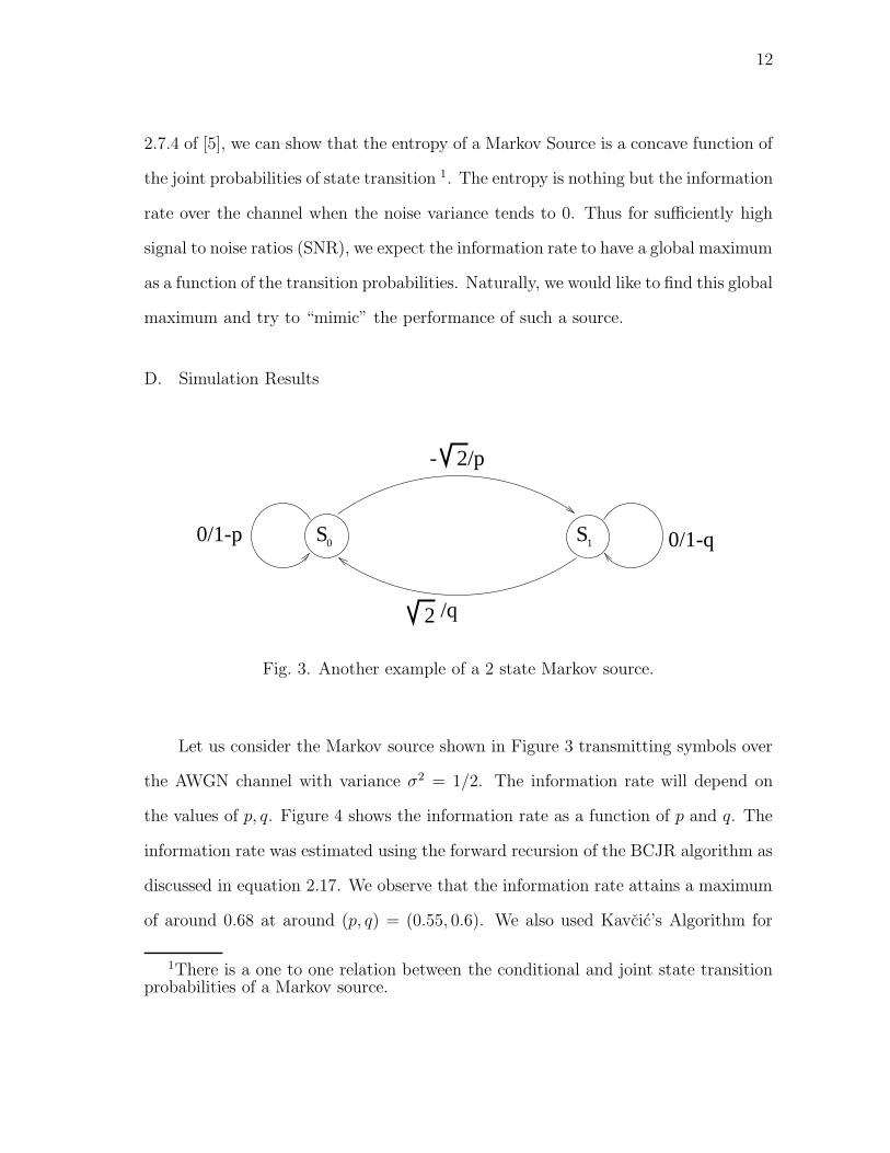
D. Simulation Results

2

2

S S0 10/1-p 0/1-q

/q

/p-

Fig. 3. Another example of a 2 state Markov source.

Let us consider the Markov source shown in Figure 3 transmitting symbols over

the AWGN channel with variance σ2 = 1/2. The information rate will depend on

the values of p, q. Figure 4 shows the information rate as a function of p and q. The

information rate was estimated using the forward recursion of the BCJR algorithm as

discussed in equation 2.17. We observe that the information rate attains a maximum

of around 0.68 at around (p, q) = (0.55, 0.6). We also used Kavcic’s Algorithm for

1There is a one to one relation between the conditional and joint state transitionprobabilities of a Markov source.

13

00.2

0.40.6

0.81

0

0.5

10

0.2

0.4

0.6

0.8

pq

Info

rmat

ion

rate

Fig. 4. Information rate of the source in Figure 3 as a function of p and q at a noise

variance of σ2 = 1/2.

the same setup and found that the optimal probability transition matrix is given by

P =

0.42 0.58

0.58 0.42

. (2.26)

The maximal value of information rate estimated is 0.676. Thus we find that both

the results agree with each other and hence Kavcic’s algorithm is verified to perform

in this case.

The selection of the particular Markov source depicted in Figure 3 may seem

arbitrary. But our motivation for selecting this source will become clear when we

discuss the applications of Kavcic’s algorithm for partial response channels in the

next chapter.

14

CHAPTER III

CHANNEL CAPACITY

In this chapter we will be reviewing methods of estimating the capacity of partial

response channels.

A. Lower Bounds

The lower bounds discussed in this section are derived from the idea that any achiev-

able information rate by a Markov source on a partial response channel is a lower

bound to the capacity. Before we proceed, it would be helpful to introduce the concept

of a “super source.”

Let us consider a Markov source at the input of a partial response channel. We

can visualize the Markov source and the channel trellis together as a super Markov

source over an AWGN channel. Note that the symbols at the output of the source

will not remain binary. For example the super source formed by the Markov source

in Figure 2 over the (1 − D)/√

2 channel is given by Figure 3.

1. Symmetric Information Rate

A scheme for estimating the uniform input information rate was proposed indepen-

dently in [12] and [13]. The binary i.i.d. source can be visualized as a single state

Markov source. This can be combined with the channel trellis to form a super source.

The information rate of this super source over the AWGN channel can be estimated

by using the forward recursion of BCJR algorithm (refer equation 2.17). This is of-

ten referred to as the symmetric information rate (SIR) or the i.i.d. capacity of the

channel.

In [12], the authors demonstrate that interleaved random binary codes can achieve

15

rates close to the SIR over partial response channels. In [14], the authors use the tools

of density evolution to design Low Density Parity Check (LDPC) Codes which have

thresholds very close to the SIR of the channel. Thus the SIR of a channel serves as a

benchmark for the performance of codes over partial response channels. In Chapters

IV and V we review/design codes which perform better than the SIR bound.

2. Extension of Kavcic’s Algorithm for Partial Response Channels

Kavcic’s algorithm tries to maximize the information rate of Markov sources over

AWGN channel. Thus it can be used to optimize the transition probabilities of the

super source to maximize its information rate. This will again serve as a lower bound

to the channel capacity.

S S

S

1-1 -11

11S-1-1

1/q

-1/p

-1/1-q

-1/1-q

-1/p

1/1-p

1/q

1/1-p

Fig. 5. Super source for Markov source in Figure 2 over 1−D+0.8D2/√

2.64 channel.

The noiseless output symbols are not shown for the sake of clarity.

However, Kavcic’s algorithm requires that the transition probabilities of the

source should be independent of each other. This may not be true always. For

16

example the super source for the Markov source given in Figure 2 over the (1 − D +

0.8D2)/√

2.64 channel (Figure 5) has transition probabilities which are interdepen-

dent.

In most of the Markov sources, there are 2m states, corresponding to the last m,

binary bits transmitted. For such Markov sources, the super source will not contain

any linearly dependent transition probabilities if the length of the channel is ≤ m+1.

A certain class of such Markov sources are called nth order channel extensions, where

n is a positive integer. The concept of channel extension is motivated from the

concept of source extensions as defined in [10]. The nth order channel extension of a

channel has the same number of states as the channel trellis. However the branches

correspond to the length n sequences. For example the source in Figure 2 is the 1st

order extension for any channel of length 2 (specifically the (1 − D)/√

2 channel).

The 3rd order channel extension is shown in Figure 6.

11111-1

1-1-11-11

11111-1

1-1-11-11

-1-1-1-11-111-11-1-1 -1-1-1

-11-111-11-1-1

S S0 1

Fig. 6. 3rd extension of a channel with length 2. Note that each branch in the figure

represents 4 possible branches in the actual source.

Optimized higher order channel extensions are expected to perform better than

the 1st order channel extension. Thus, while the source in Figure 2 achieves an

17

information rate of 0.676 over the (1 − D)/√

2 channel at Es/N0 = 0 dB, the source

in Figure 6 achieves an information rate of about 0.71 bits per channel use.

However, one would not like to restrict oneself just to channel extensions while

searching for the optimal source. Thus extension of Kavcic’s algorithm, to optimize

sources with linearly dependent transition probabilities is highly desirable. How to

do so (by extending the proof of Appendix A), is still not clear.

B. Upper Bounds to Channel Capacity

1. Waterfilling Theorem

The Water Filling Theorem (Section 10.5 [5]) states that for continuous alphabet

sources over partial response channels, the information rate is maximized if we dis-

tribute the input power (spectral density) as given by the waterfilling over inverse of

channel frequency response. The result is intuitive in the sense that we are trying to

“pump” in more information through the frequency band in which channel is good.

An example of a water filling spectrum for the (1−D)/√

2 channel is shown in Figure

7.

The waterfilling capacity of the channel is given by

C =∫

1

2log2(1 +

(ν − N(f))+

N(f))df, (3.1)

where ν is such that∫

(ν − N(f))+df is the total input power. The function (.)+ is

defined as

(x)+ =

x if x ≥ 0

0 if x < 0(3.2)

Since the waterfilling theorem is valid for the case of continuous alphabet sources,

min.(1, waterfilling capacity) will be an upper bound to the capacity of the channel.

18

0.1 0.2 0.3 0.4 0.5 0.6 0.7 0.8 0.90

0.5

1

1.5

2

2.5

3

frequency(f)

Wat

erfil

ling

Spe

ctru

m

signal spectrumvariance/||g(f)||2

Fig. 7. Waterfilling spectrum over 1-D channel with Es/N0 = 0 dB.

2. Vonotobel-Arnold Upper Bound

In [15], the authors present a method to estimate an upper bound for the channel

capacity of a partial response channel with binary input. The method is motivated

by Problem 4.17 of [1]. Here, we discuss the generalization of the problem.

Consider a discrete source X with probability distribution P0(X), as an input to

a discrete memoryless channel. Let Y be the discrete symbols observed at the output

of the channel. Then

I(X; Y ) ≤ C ≤ max

kI(x = k; Y ). (3.3)

If the distribution P0(X) in the above equation is capacity achieving, then the in-

equalities turn into equalities. Thus we expect that as the probability distribution of

the source tends towards a capacity achieving distribution, the bound to the chan-

19

nel capacity becomes tighter. The generalization of equation 3.3 to partial response

channels is

limN→∞

1

NI(XN

1 ; Y N1 ) ≤ C ≤ lim

N→∞

max

uN1

1

NI(xN

1 = uN1 ; Y N

1 ). (3.4)

Thus the problem of finding an upper bound to the capacity reduces to finding a

“good” source and finding a sequence uN1 , such that the information conveyed by

that sequence is the maximum.

In their paper, [15], Vontobel et al. use Markov source optimized by Kavcic’s

Algorithm. Then they perform a trellis based search to find the “best” sequence. The

algorithm is quite complex to implement and at low rates, the upper bound is very

close to the waterfilling capacity.

20

CHAPTER IV

MATCHED INFORMATION RATE CODES

In [16], Kavcic, et al. design codes that achieve rates higher than the symmetric infor-

mation rate of a partial response channel. The code consists of serially concatenated

outer LDPC codes with an inner trellis code, as shown in Figure 8.

LDPCcoderate=r

LDPCcoderate=r Decoder

LDPC

Decoder

LDPC

+

Partial response channel

g(D)Y

Z

i

i

Xi

Trellis Code

rate=k/n

. . k

LD

PC c

odes

. .

DecoderTrellis

. k L

DPC

dec

oder

s .

Pseudo Channel

1

k

Fig. 8. Structure of the matched information rate code.

The inner trellis code tries to “mimic” the sub optimal Markov source derived

from Kavcic’s rate optimizing algorithm as discussed in Section A.2 of Chapter 3.

With properly optimizing the outer LDPC codes, we can surpass the i.i.d. capacity

of the channel. In this chapter we will discuss the results of [16].

A. Design of Inner Trellis Code

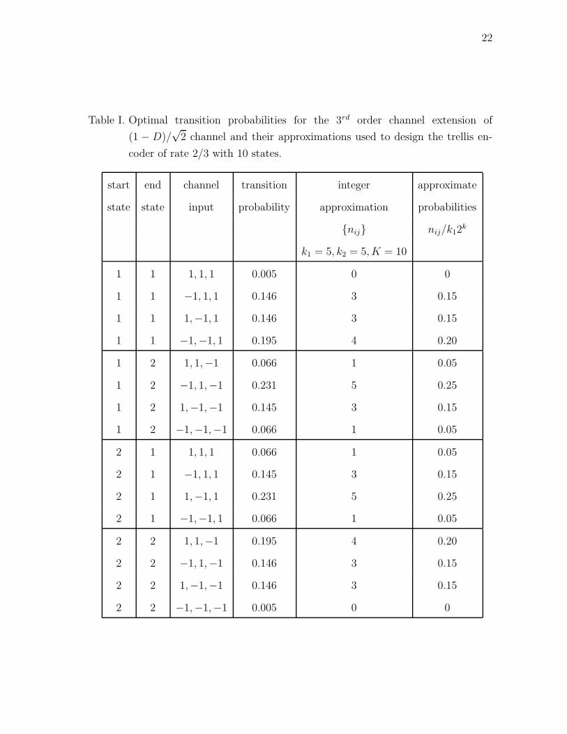
Let us consider the 3rd order extension of the 1 − D channel. We optimize the

transition probabilities for various SNR’s, to maximize the information rate over the

(1 − D)/√

2 channel. The optimal source achieves an information rate of 0.5 at

Es/N0 = −2.7 dB. The optimal transition probabilities of this source are listed in

21

Table I. Our aim is to “mimic” the performance of this source by a rate k/n trellis

code, so as to achieve an overall rate of 0.5 at Es/N0 close to −2.7 dB.

A rate k/n trellis code is characterized by K states. Each state has 2k branches

coming out of it (corresponding to 2k different possible inputs). Each branch is

mapped to a binary n-tuple which is the output of the particular branch transition.

Since we are trying to mimic the 3rd extension of the channel we will choose n = 3.

We would like the inner code rate k/n, to be greater than the target rate (= 0.5).

Thus we choose k = 2.

We will split the M(= 2) states of the 3rd order extension into k1 and k2 states

so that they minimize the Kullback Leibler Distance1 [5] D(κ||µ), where κ is the

probability distribution (k1

K, · · · , kM

K), with the constraint that

∑ki ≤ K. The µi’s

are the steady state probabilities of the states of the Markov source.

Now, corresponding to each state i of the Markov Source we have ki2k branches

in the encoder. We would like to choose a set of integers {nil} where l = 0, 1, . . .

such that the transition probabilities of the branches emanating from state i are

approximated by the fractions { nil

ki2k }. To do so we minimize the Kullback Leibler

Distance between the transition probabilities of branches originating from state i and

the above fractions. The problem of finding the approximate encoder is solved by

solving the 2 optimization problems of minimizing the Kullback Leibler Distance.

However the solution may not be unique. Out of all the possible set of solutions

we choose the one which minimizes∑

i κiD({Pil}||{ nil

ki2k }). The results for such an

optimization are shown in Table I.

1The Kullback Leibler distance between 2 probability mass functions p(.) and q(.)

is defined as D(p||q) =∑

x p(x) log2p(x)q(x)

. Furthermore, D(p||q) is 0 iff p = q.

22

Table I. Optimal transition probabilities for the 3rd order channel extension of

(1 − D)/√

2 channel and their approximations used to design the trellis en-

coder of rate 2/3 with 10 states.

start end channel transition integer approximate

state state input probability approximation probabilities

{nij} nij/k12k

k1 = 5, k2 = 5, K = 10

1 1 1, 1, 1 0.005 0 0

1 1 −1, 1, 1 0.146 3 0.15

1 1 1,−1, 1 0.146 3 0.15

1 1 −1,−1, 1 0.195 4 0.20

1 2 1, 1,−1 0.066 1 0.05

1 2 −1, 1,−1 0.231 5 0.25

1 2 1,−1,−1 0.145 3 0.15

1 2 −1,−1,−1 0.066 1 0.05

2 1 1, 1, 1 0.066 1 0.05

2 1 −1, 1, 1 0.145 3 0.15

2 1 1,−1, 1 0.231 5 0.25

2 1 −1,−1, 1 0.066 1 0.05

2 2 1, 1,−1 0.195 4 0.20

2 2 −1, 1,−1 0.146 3 0.15

2 2 1,−1,−1 0.146 3 0.15

2 2 −1,−1,−1 0.005 0 0

23

Thus all the 3-tuple outputs of the branches are derived by solving the opti-

mization problem. However there are many ways by which the same branches may

be connected between different states in the trellis encoder. To give an estimate of

numbers, there are 540 possible permutations of branches possible for the source with

parameters represented in Table I. Which permutation do we choose? We randomly

select a large number of possible permutations (say 104) and evaluate the i.i.d ca-

pacity of the trellis for that permutation. We select the permutation which gives the

highest i.i.d. capacity.

B. Outer Code Design

The inner trellis code designed in the previous section requires that the input to it

should be i.i.d. binary digits. Further we want the rate of the outer code to be 3/4.

Ideally speaking these 2 conditions cannot be met simultaneously. However, LDPC

codes with large block lengths can produce approximately i.i.d. sequences.

We can visualize the output of the outer code as an input to a pseudo channel

(Figure 8), where the pseudo channel is the combination of inner trellis code, the

partial response channel and the soft output trellis decoder. The input to the pseudo

channel is a k-tuple. Thus we can design k LDPC codes for this pseudo channel.

At the decoder we will employ k corresponding LDPC decoders. The first decoder

decodes using the first bit in each k tuple without assuming anything about the other

bits. The second decoder decodes using the second bit in each k tuple assuming the

first bit is successfully decoded (The trellis decoder gives an updated estimate on the

second bit assuming the first bit is known), etc.

The rate of the outer code is r = 1k

∑

i ri, where ri’s are defined by

r1 = limN→∞

1

NI(XN

1 (1);YN1 )

24

r2 = limN→∞

1

NI(XN

1 (2);YN1 |XN

1 (1))

...

rk = limN→∞

1

NI(XN

1 (k);YN1 |XN

1 (1), · · · , XN1 (k − 1)), (4.1)

where XN1 (l) denotes the bits in the positions l, l + k, l + 2k, · · ·.

The degree sequences of the LDPC codes are optimized so that we get the lowest

thresholds for all the k codes, while their information rates as given by equation

4.1 are close to the target rate. The tools of density evolution as discussed in [14,

?] are used for this optimization. The overall threshold of the codes is Es/N∗

0 =

max.(Es/N0∗

1, Es/N0∗

2 · · · , Es/N0∗

k). Here Es/N0∗

l is the threshold of the individual

LDPC code.

In [16], the authors design the optimal outer irregular LDPC codes for the exam-

ple we are considering. The codes were designed for rate 3/4 and had thresholds 0.17

dB away from the inner trellis code capacity at target rate of 0.5. This scheme had

a gain of around 0.25 dB over the i.i.d capacity of (1−D)/√

2 channel. The authors

showed similar gains over the i.i.d capacity of the (1−D + 0.8D2)/√

2.64 at a target

rate of 0.5.

C. Summary

The matched information rate coding scheme discussed in this chapter has been shown

to achieve high target rates over partial response channels with a considerable gain

over the i.i.d capacity of the channel. However both the design process and imple-

mentation of the codes is quite complex (practically un-implementable).

25

CHAPTER V

MATCHED SPECTRUM CODES

A. Motivation

If the PSD of the encoded data matches the waterfilling spectrum, the information

rate is maximized.1 Thus, we expect the codes to perform better if their PSD resem-

bles the waterfilling spectrum.

In Section D of Chapter II, we found the optimum transition probabilities of a

2 state Markov source over the (1−D)/√

2 channel (equation 2.26). In Figure 9, we

plot the power spectral density of that source. We notice that the PSD of the source

0 0.05 0.1 0.15 0.2 0.25 0.3 0.35 0.4 0.45 0.50.1

0.15

0.2

0.25

0.3

0.35

0.4

0.45

0.5

Frequency

Pow

er S

pect

ral D

ensi

ty

Fig. 9. Power Spectral Density of the Markov source defined by equation 2.26.

1This is usually not doable for finite alphabet sources.

26

peaks at high frequency and thus in some sense tries to match the frequency response

of the channel. This gives us an intuitive motivation that for optimal binary sources

over partial response channels the PSD of the source should in some sense match the

channel frequency response. In [17], the authors show substantial increase than the

i.i.d. capacity of the channel for block codes with spectrum matched to the channel

response.

1. Performance Index of Codes

Now let us consider the problem of encoding for partial response channels for very

low rates 1/n with n → ∞. For each binary bit {±1}, we should assign a binary

n-tuple. Obviously these n tuples should be such that the output of these n-tuple’s

from the channel filter should have maximum energy. Thus again we are trying

to match the PSD with the channel frequency response. The best we can hope to

achieve is when the spectrum of the data bits is an impulse at the frequency where

the channel frequency response is maximum. Thus for any coding scheme we can

define a performance index (p.i.)

p.i. =Power of the sequence at the oputput of noiseless partial response channel

Input Power × max|g(f)|2 .

(5.1)

We expect that codes with higher p.i. should perform better than codes with lower

p.i. (at least asymptotically for low rates).

In the previous chapter we discussed a coding scheme in which an encoder tries

to “mimic” the performance of an optimal Markov source. The technique led to very

complex encoders. However, the arguments presented in this section motivate that we

can design our codes to match the channel spectrum and achieve good performance.

It would be beneficial if we have some techniques by which we can design simple

27

encoders which match the channel spectrum. In this chapter we discuss such a scheme

for spectrum matching. The scheme is expected to perform better for low rates.

B. Cavers-Marchetto Coding Technique

D D D D D D 1 D D D D D D 1D D D 1 D D D D D . . .. . .

Block of length Nb

Flag bits

D: data bits

Fig. 10. Coding technique of Cavers-Marchetto

In [2], the authors describe a coding technique of rate (Nb − 1)/Nb, where Nb is

an integer, to shape the spectrum of the code. Let us consider a binary data source,

in which the data bits are divided into blocks of length Nb − 1 (Figure 10). We add

a constant flag bit, say “1”, at the end of each block. We now have blocks of length

Nb. With the ith such block we associate a flag index F (i), where F (i) ∈ {−1, +1}.

Before transmitting over the channel, the ith block is multiplied by the flag index

F (i). We have the freedom to select the flag indices to shape the spectrum of the

code.

Suppose that we want the spectrum of the encoded stream to match a filter

g1(n). We want to choose the flag indices so that the energy of the encoded stream

when passed through g1(n) is maximum. A symbolic representation of this idea is

shown in Figure 11. In [2], the authors solve this problem by formulating a Viterbi

type algorithm at the encoder.

We will equivalently solve this problem by representing the source as a trellis

encoder. In the encoder, there are 2Length(g1(n))−1 states corresponding to the last

28

Data stream

with flag bitsBlockinversion

to channel

g(n)1

Σ(.)

Flagindices

Maximize

2

Fig. 11. Structure of Cavers-Marchetto encoder.

Length(g1(n)) − 1 bits transmitted over the channel. Each branch in the trellis rep-

resents a Nb − 1 binary-tuple input and an output of length Nb which is transmitted

over the channel. Thus each branch will have a transition probability of 2−(Nb−1).

An example of the rate 1/2 code matched to g1(D) = 1 − D is shown in Figure 12.

However it may turn out that the encoder is not unique. In which case we select the

encoder for which the average distance between the outputs of branches originating

from a state is maximum (at the output of the channel).

S S0 1

1/11

1/-1-1

-1/-11-1/1-1

Fig. 12. Rate 1/2 code matched to 1 − D.

The advantage of representing the source as a trellis encoder is that we can

29

estimate the information rate at the output of the channel. Figure 13 shows the

performance of codes matched to 1−D when transmitted over a (1−D)/√

2 channel.

We also show the i.i.d capacity of the channel for comparison. We notice that for low

rate regions these encoders surpass the i.i.d. capacity.

−4 −2 0 2 4 6 8 100

0.1

0.2

0.3

0.4

0.5

0.6

0.7

0.8

0.9

1

Eb/N

0 (dB)

Info

rmat

ion

rate

i.i.d. capacityrate 2/3rate 1/2waterfilling UB

Fig. 13. Performance of codes matched to 1 − D, when transmitted over (1 − D)/√

2

channel (Cavers-Marchetto technique).

C. Generalization of Cavers-Marchetto Technique

We ask ourselves the following questions. Is the Cavers-Marchetto technique the ideal

way to form a trellis encoder to maximize the energy of an encoded stream through

a filter g1(n)? Can the Cavers-Marchetto technique be generalized to form encoders

for any arbitrary rate?

30

The questions above can be answered by the following “greedy” algorithm to

design a rate k/n trellis encoder.

1. Consider a trellis with 2Length(g1(n))−1 states. Each state corresponds to the

last Length(g1(n)) − 1 bits sent through the channel.

2. There are 2k branches originating from each state. Assign an input k-tuple to

each branch.

3. There are 2n possible output n-tuples for each state. Out of these, select 2k

possible outputs which when passed through g1(n), have the maximum energy.

Assign 2k such n-tuples to all the branches originating from the particular state.

4. Terminate the branches into the states corresponding to the last Length(g1(n))−

1 bits transmitted.

5. Discard any redundant states i.e., states with no incoming branches.

6. If more than one optimal trellis encoder is possible, select the one for which

the average distance between the outputs of branches originating from a state

is maximum (at the output of the channel).

It is expected that the generalized algorithm will perform better if g1(D) resembles

the channel transfer function. The simulations confirmed the same. In Figure 14, we

show the normalized transfer functions of various filters that we will be using.

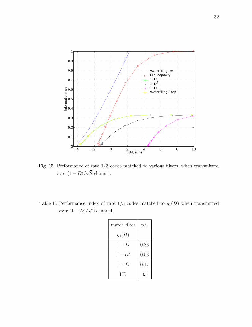
The performance of rate 1/3 codes over a (1−D)/√

2 channel, designed by using

the generalized scheme and matched to various different filters is shown in Figure 15.

We also evaluated the performance index of each code and tabulated them in Table

II. We notice from Table II and Figure 15, that asymptotically the codes with higher

performance index perform better. In the figure we have also shown the performance

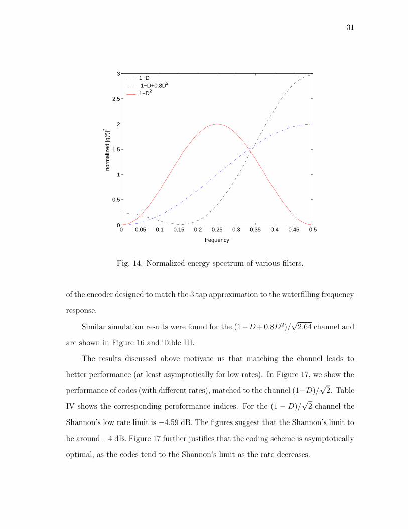
31

0 0.05 0.1 0.15 0.2 0.25 0.3 0.35 0.4 0.45 0.50

0.5

1

1.5

2

2.5

3

frequency

norm

aliz

ed |g

(f)|

2

1−D 1−D+0.8D2

1−D2

Fig. 14. Normalized energy spectrum of various filters.

of the encoder designed to match the 3 tap approximation to the waterfilling frequency

response.

Similar simulation results were found for the (1−D+0.8D2)/√

2.64 channel and

are shown in Figure 16 and Table III.

The results discussed above motivate us that matching the channel leads to

better performance (at least asymptotically for low rates). In Figure 17, we show the

performance of codes (with different rates), matched to the channel (1−D)/√

2. Table

IV shows the corresponding peroformance indices. For the (1 − D)/√

2 channel the

Shannon’s low rate limit is −4.59 dB. The figures suggest that the Shannon’s limit to

be around −4 dB. Figure 17 further justifies that the coding scheme is asymptotically

optimal, as the codes tend to the Shannon’s limit as the rate decreases.

32

−4 −2 0 2 4 6 8 100

0.1

0.2

0.3

0.4

0.5

0.6

0.7

0.8

0.9

1

Eb/N

0 (dB)

Info

rmat

ion

rate

Waterfilling UBi.i.d. capacity1−D1−D2

1+DWaterfilling 3 tap

Fig. 15. Performance of rate 1/3 codes matched to various filters, when transmitted

over (1 − D)/√

2 channel.

Table II. Performance index of rate 1/3 codes matched to g1(D) when transmitted

over (1 − D)/√

2 channel.

match filter p.i.

g1(D)

1 − D 0.83

1 − D2 0.53

1 + D 0.17

IID 0.5

33

−6 −4 −2 0 2 4 6 8 100

0.1

0.2

0.3

0.4

0.5

0.6

0.7

0.8

0.9

1

Eb/N

0 (dB)

Info

rmat

ion

rate

Waterfilling UBi.i.d. capacity1−D+0.8D2

1−D2

1+DWaterfilling 3 tap

Fig. 16. Performance of rate 1/3 codes matched to various filters, when transmitted

over (1 − D + 0.8D2)/√

2.64 channel.

Table III. Performance index of rate 1/3 codes matched to g1(D) when transmitted

over (1 − D + 0.8D2)/√

2.64 channel.

match filter p.i.

g1(D)

1 − D + 0.8D2 0.71

1 − D2 0.23

1 + D 0.1

IID 0.34

34

−5 −4 −3 −2 −1 0 1 20

0.05

0.1

0.15

0.2

0.25

0.3

0.35

0.4

0.45

0.5

Eb/N

0 (dB)

Info

rmat

ion

rate

Waterfilling UBi.i.d. capacityrate2/3rate 1/2rate1/3rate 1/4rate 1/5

Fig. 17. Performance of codes matched to (1 − D)/√

2, when transmitted over

(1 − D)/√

2 channel.

Table IV. Performance index of codes matched to (1−D)/√

2 when transmitted over

(1 − D)/√

2 channel.

rate p.i.

2/3 0.75−

1/2 0.75+

1/3 0.83

1/4 0.87

1/5 0.90

35

Now let us reconsider the code design problem and exploit the results shown in

Figure 17. Suppose that we target a rate of 0.1 over the channel. We notice that if we

use an inner trellis code of rate 1/3 matched to (1 − D)/√

2, then we expect to gain

around 1.6 dB with respect to the i.i.d capacity. Thus in the next section we will be

discussing how to design the outer LDPC code for the inner rate 1/3 code over the

(1 − D)/√

2 channel.

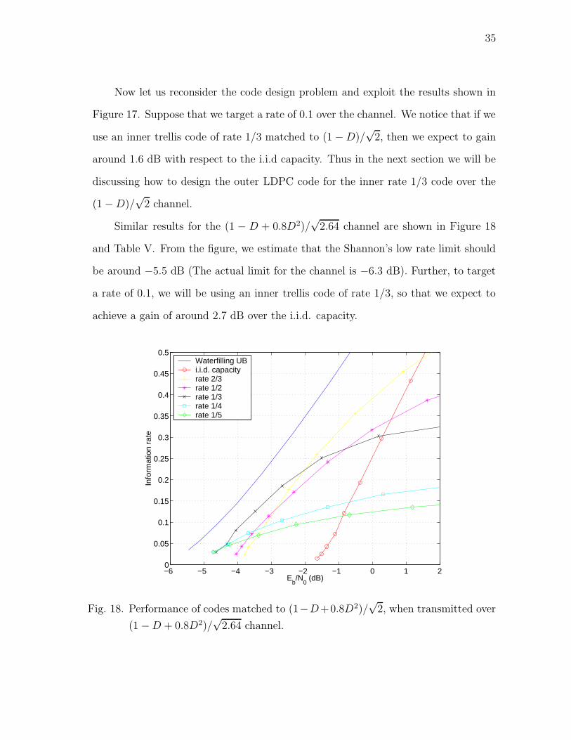
Similar results for the (1 − D + 0.8D2)/√

2.64 channel are shown in Figure 18

and Table V. From the figure, we estimate that the Shannon’s low rate limit should

be around −5.5 dB (The actual limit for the channel is −6.3 dB). Further, to target

a rate of 0.1, we will be using an inner trellis code of rate 1/3, so that we expect to

achieve a gain of around 2.7 dB over the i.i.d. capacity.

−6 −5 −4 −3 −2 −1 0 1 20

0.05

0.1

0.15

0.2

0.25

0.3

0.35

0.4

0.45

0.5

Eb/N

0 (dB)

Info

rmat

ion

rate

Waterfilling UBi.i.d. capacityrate 2/3rate 1/2rate 1/3rate 1/4rate 1/5

Fig. 18. Performance of codes matched to (1−D+0.8D2)/√

2, when transmitted over

(1 − D + 0.8D2)/√

2.64 channel.

36

Table V. Performance index of codes matched to (1−D + 0.8D2)/√

2.64 when trans-

mitted over (1 − D + 0.8D2)/√

2.64 channel.

rate p.i.

2/3 0.58

1/2 0.63

1/3 0.71

1/4 0.82

1/5 0.85

D. Design of Outer Irregular LDPC Codes

In this section we will concentrate on the design of an outer irregular LDPC code of

rate 0.3. The LDPC code design problem can be viewed as a code design problem

for the pseudo channel (Figure 8) where the pseudo channel consists of a trellis en-

coder of rate 1/3, a partial response channel, an AWGN source and a trellis decoder.

The design technique follows from the Extrinsic Information Transfer (EXIT) chart

technique as discussed in [18]. A good exposition of extrinsic information and EXIT

charts can be found in [19, 20]. A basic introduction to LDPC codes can be found in

[21]. Here, we will just mention how we used the concepts.

We use equation 2.7 to estimate the log likelihood ratios of the bits transmitted

over the pseudo channel. We do so by using the BCJR algorithm. A typical distri-

bution of the log likelihood ratios (LLR) is shown in Figure 19. We approximate the

distribution to be Gaussian to ease calculations.

The LDPC decoder can be visualized as an iterative decoder for a serially con-

catenated code with an inner repeat code (Variable node - VND) and outer single

37

−6 −4 −2 0 2 4 6 80

500

1000

1500

2000

2500

Log Likelihood Ratios

Occ

uren

ces

Fig. 19. Histogram of the log likelihood ratio values from the pseudo channel over the

partial response channel (1 − D + 0.8D2)/√

2.64 for Eb/N0 = −3.55 dB.

38

parity check codes (Check node - CND). For the decoder to successfully converge, the

EXIT chart at the variable node decoder should lie above the EXIT chart of the check

node decoder. We use the approximations mentioned in [18] to formulate the Exit

chart curves as a function of the standard deviation of the LLR values, the degree

sequence and the a priori information. We then optimized the degree distribution to

maximize the rate for a particular standard deviation (and hence a particular Eb/N0),

under the constraint that the VND curve should lie above the CND curve. We repeat

this procedure for various values of Eb/N0 until we get a rate close to the target rate.

Hence the threshold SNR is evaluated.

1. Results

The trellis code capacity of the rate 1/3 code for the (1−D)/√

2 channel is Eb/N0 =

−2.82 dB at a rate of 0.1 (Figure 17). We designed the LDPC code with rate 0.3

and threshold Eb/N0 = −2.6 dB. Thus the design is better than the i.i.d. capacity

of the channel by 1.4 dB. The code had a check node degree dc = 5. The generating

function λ(x) is shown in the Table VI and the EXIT chart plotted in Figure 20.

Similar results for the (1 − D + 0.8D2)/√

2.64 channel, are shown in Figure 21

and Table VII. The trellis code capacity was 0.1 at Eb/N0 = −3.81 dB. The designed

LDPC code has a threshold of −3.55 dB. With respect to the i.i.d. capacity, this

implies a gain of 2.59 dB.

39

0 0.1 0.2 0.3 0.4 0.5 0.6 0.7 0.8 0.9 10.1

0.2

0.3

0.4

0.5

0.6

0.7

0.8

0.9

1

IA,VND

,IE,CND

I E,V

ND,I A

,CN

D

Check node EXIT chartVar. node EXIT chart

Fig. 20. EXIT chart for the check regular LDPC code with rate 0.3 and threshold

Eb/N0 = −2.6 dB. This code is deigned for the (1 − D)/√

2 channel.

Table VI. Degree sequence for the rate 0.3 LDPC code for the (1 − D)/√

2 channel.

It has a threshold of Eb/N0 = −2.6 dB.

i λi ρi

2 0.2617

3 0.3566

5 1

6 0.0236

8 0.1655

18 0.1926

40

0 0.1 0.2 0.3 0.4 0.5 0.6 0.7 0.8 0.9 10.1

0.2

0.3

0.4

0.5

0.6

0.7

0.8

0.9

1

IA,VND

,IE,CND

I E,V

ND,I A

,CN

D

Check Node EXIT chartVar. node EXIT chart

Fig. 21. EXIT chart for the check regular LDPC code with rate 0.3 and threshold

Eb/N0 = −3.55 dB. This code is designed for the (1 − D + 0.8D2)/√

2.64

channel.

Table VII. Degree sequence for the rate 0.3 LDPC code for the (1−D+0.8D2)/√

2.64

channel. It has a threshold of Eb/N0 = −3.55 dB.

i λi ρi

2 0.2621

3 0.3592

5 1

6 0.0084

8 0.1831

18 0.1872

41

CHAPTER VI

CONCLUSION

The main contributions of this thesis can be summed up as follows:

1. By simulations, we verified that matching the spectrum of the data stream with

the channel frequency response leads to better information rates.

2. We provided a qualitative argument for the optimality of the encoder design

technique presented in Section C of Chapter V for low rates.

3. We formulated the concept of performance index of an encoder and verified its

validity by simulation results.

4. Motivated by the above results, we designed a serially concatenated coding

scheme with an outer irregular LDPC code and an inner matched spectrum

trellis code. The performance was found to be 1.4 dB better than the i.i.d.

capacity of the channel for a target rate of 0.1 for the (1−D)/√

2 channel. For

the (1 − D + 0.8D2)/√

2.64 channel, the performance was found to be 2.59 dB

better. The coding scheme is considerably easier to implement than the existing

schemes.

A. Future Work

We believe that the following problems may be very interesting to investigate.

1. We believe that it can be analytically shown that there is a threshold SNR for

every channel, so that the information rate as a function of transition proba-

bilities of a Markov source, will have just one global maximum, if the SNR is

42

greater than the threshold. This thought is motivated by the discussion at the

end of Section C of Chapter II.

2. It would be beneficial to extend Kavcic’s algorithm for the case when the tran-

sition probabilities of the Markov source are linearly dependent on each other.

This would help us optimize any Markov source over any partial response chan-

nel. Perhaps the proof shown in Appendix A may be extended.

3. In [22], the authors find the closed form expression for the power spectral density

of certain special Markov sources. However, in general there is no closed form

expression for the power spectral density of a Markov source. The working in

Section 4.4.3 of [23] is pretty confusing, and so we have included the general

derivation of the power spectral density of a Markov source in Appendix B.

Designing Markov sources so that the PSD matches a given function in the

frequency domain is still an open problem.

4. We considered the problem of code designing for 2 channels. There was a wide

difference in the gain over the i.i.d. capacity for the 2 channels. It would be

interesting to investigate, for which channels should the proposed coding scheme

perform better as compared to other channels.

43

REFERENCES

[1] R. G. Gallager, Information Theory and Reliable Communication, New York:

John Wiley and Sons Inc., 1968.

[2] J. K. Cavers and R. F. Marchetto, “A New Coding Technique for Spectral Shap-

ing of Data,”IEEE Transactions on Communications, Vol. 40, No. 9, pp. 1418-

1422, Septmeber 1992.

[3] R. Karabed and P. H. Siegel, “Matched Spectral-Null Codes for Partial-Response

Channels,”IEEE Transactions of Information Theory, Vol. 37, No. 3, pp. 818-855,

May 1991.

[4] B. F. Uchoa Filho and M. A. Herro, “Good Convolutional Codes for Precoded

(1−D)(1 + D)n Partial-Response Channels,”IEEE Transactions on Information

Theory, Vol. 43, No. 2, pp. 441-453, March 1997.

[5] J. A. Thomas and T. M. Cover, Elements of Information Theory, New York:

John Wiley and Sons Inc., 1991.

[6] L. R. Bahl, J. Cocke, F. Jelinek and J. Raviv, “Optimal Decoding of Linear

Codes for Minimizing Symbol Error Rate,”IEEE Transactions on Information

Theory, Vol. 20, pp. 284-287, March 1974.

[7] A. Kavcic, “On the Capacity of Markov Sources over Noisy Channels,”in Pro-

ceedings IEEE Global Communications Conference 2001, San Antonio, Texas,

November 2001, pp. 2997-3001.

[8] S. Arimoto, “An Algorithm for Computing the Capacity of Arbitrary Discrete

Memoryless Channels,”IEEE Transactions on Information Theory, Vol. IT-18,

No. 1, pp. 14-20, January 1972.

44

[9] R. E. Blahut, Digital Transmission of Information, Reading, Massachusets:

Addison-Wesley Publishing Company, 1990.

[10] B. H. Marcus, P. H. Siegel and J. K. Wolf, “Finite-State Modulation Codes for

Data Storage,”IEEE Journal on Selected Areas in Communications, Vol. 10, No.

1, pp. 5-37, January 1992.

[11] P. O. Vonotobel,“Maximization of the Information Rate under Constraints,”,

May 2001, (Personal Collection, D. Kumar).

[12] H. D. Pfister, J. B. Soriaga and P. H. Siegel, “On the Achievable Information

Rates of Finite State ISI Channels,”in Proceedings IEEE Global Communica-

tions Conference 2001, San Antonio, Texas, November 2001, pp. 2992-2996.

[13] D. M. Arnold and H. A. Loeliger, “On the Information Rate of Binary Input

Channels with Memory,”in Proceedings IEEE International Conference on Com-

munications 2001, Helsinki, Finland, June 2001, pp. 2692-2695.

[14] N. Varnica and A. Kavcic, “Optimized Low-Density Parity Check Codes for

Partial Response Channels,”in IEEE Communications Letters, Vol. 7, No. 4, pp.

168-170, April 2003.

[15] P. O. Vontobel and D. M. Arnold, “An Upper Bound on the Capacity of Chan-

nels with Memory and Constraint Input,”in Information Theory Workshop 2001,

Cairns, Australia, September 2001, pp. 147-149.

[16] X. Ma, N. Varnica and A. Kavcic, “Matched Information Rate Codes for Binary

ISI channels,”in Proceedings of IEEE International Symposium on Information

Theory 2002, Lausanne, Switzerland, July 2002, p. 269.

45

[17] D. N. Doan and K. R. Narayanan, “Design of Good Low Rate Codes for ISI

Channels Based on Spectral Shaping,”to appear at the 3rd International Sym-

posium on Turbo Codes and Related Topics, Brest, France, September 2003.

[18] S. ten Brink, G. Kramer and A. Ashikhmin “Design of Low-Density Parity-Check

Codes for Multi-Antenna Modulation and Detection,” submitted to the IEEE

Transactions on Communications, June 2002 (Personal collection, D. Kumar).

[19] C. Berrou, A. Glavieux and P. Thitimajshima, “Near Shannon Limit Error-

Correcting Coding and Decoding: Turbo Codes(1),”in Proceedings IEEE Inter-

national Conference on Communications 1993, Geneva, May 1993, pp. 1064-1070.

[20] S. ten Brink, “Convergence Behavior of Iteratively Decoded Parallel Concate-

nated Codes,”IEEE Transactions on Communications, Vol. 49, No. 10, pp. 1727-

1737, October 2001.

[21] W. Ryan, An Introduction to Low-Density Parity-Check Codes, hand written

lecture notes, April 2001 (Personcal collection, D. Kumar).

[22] A. Gallopoulos, C. Heegard and P. H. Siegel, “The Power Spectrum of Run-

Length-Limited Codes,”IEEE Transactions on Communications, Vol. 37, No. 9,

pp. 906-917, Septmeber 1989.

[23] J. G. Proakis, Digital Communications, 4th edition, New York: The McGraw-

Hill Companies, Inc., 2001.

[24] X. Ma, A. Kavcic and M. Mitzenmacher, “The Power Spectra of Good Codes

for Partial Response Channels,”accepted for IEEE International Symposium on

Information Theory 2003, Yokohama, Japan, July 2003.

46

APPENDIX A

OUTLINE OF THE PROOF OF EQUATION 2.24

We present a brief outline of the proof to equation 2.24 as given in [11]. For the sake

of completeness, let us restate the optimization problem.

Let S denote the set of states of a Markov source. Let A be the incidence matrix

of the source, i.e., Aij = 1 if the transition from state i to j is allowed, else Aij = 0.

The matrix P which maximizes the argument

V =∑

i∈S

µi

∑

j∈S

AijPij(log2 (1

Pij

) + Tij) (A.1)

under the conditions

∑

j∈S

AijPij = 1 for all i ∈ S

∑

i∈S

µiAijPij = µj for all j ∈ S

∑

i∈S

µi = 1, (A.2)

is given by

Pij =bj

bi

Aij

ρ, (A.3)

where the matrix A is defined by Aij = Aij2Tij and ρ is the maximal (real) eigenvalue

of A with eigenvector b.

Now that we have stated the problem, we set up the Lagrangian,

L =∑

i∈S

µi

∑

j∈S

AijPij(log2 (1

Pij

) + Tij)

+∑

i∈S

λi

∑

j∈S

AijPij +∑

j∈S

λ′

j(∑

i∈S

µiAijPij − µj) + λ′′∑

i∈S

µi, (A.4)

47

We need to solve the equations

∂L

∂µk

= 0 for all k ∈ S

∂L

∂Pkl

= 0 for all k, l ∈ S (A.5)

under the constraints defined by equation A.2. By some manipulation, we get

Pkl = 2λ′l−λ′

k+λ′′+TklAkl (A.6)

and∑

l∈S

Akl2Tkl2λ′

l = 2−λ′′+λ′k . (A.7)

In equation A.7, we identify Aij = Aij2Tij , b as the eigenvector with entries

bi = 2λ′i and ρ = 2−λ′′

as the eigenvalue. We thus get

AbT = ρbT . (A.8)

Thus, using equation A.8 and equation A.6 we get the desired result of equation A.3.

48

APPENDIX B

POWER SPECTRAL DENSITY OF A MARKOV SOURCE

Suppose a Markov source has n states. Let the probability transition matrix be

defined by Pij = P (st+1 = j/st = i), where st is the state of the Markov source at

time t. Let the matrix I be such that Iij is the symbol transmitted by the Markov

source for a transition from state i to j. Let Φ represent the autocorrelation function.

PSD =∞∑

k=−∞

Φ(k) ej2πkfTs

︸ ︷︷ ︸

θk

=∞∑

k=1

E(ItI∗

t+k)θk

︸ ︷︷ ︸

T1

+−1∑

k=−∞

E(ItI∗

t+k)θk

︸ ︷︷ ︸

T2

+ E(|I|2)︸ ︷︷ ︸

T3

T3 =∑

ij

µiPij|Iij|2

T1 = T ∗

2

=∞∑

k=1

∑

ij

E(ItI∗

t+k/st−1 = i; st = j)µiPijθk

=∞∑

k=1

∑

ij

IijµiPijθkE(I∗

t+k/st = j)

=∞∑

k=1

∑

ij

IijµiPijθk

∑

lm

I∗

lm[P k−1]jlPlm, (B.1)

where [P k]jl is the jlth entry of matrix P k and µi is the steady state probability of

state i.

Thus

PSD =∑

ij

µiPij|Iij|2 + 2Re[∞∑

k=1

∑

ijlm

IijµiPijθkI∗

lm[P k−1]jlPlm]. (B.2)

If Iij ∈ {−1, +1}, then the above equation reduces to

PSD = 1 + 2∞∑

k=1

∑

ijlm

IijµiPijIlm[P k−1]jlPlm cos 2πkfTs. (B.3)

49

Still we do not have a closed form expression for the power spectral density. As

discussed in [24], a good approximation is achieved if we restrict the summation of k

index in the equation above to a large finite integer.

50

VITA

Deepak Kumar was born in India on October 20, 1979. He received his Bach-

elor of Technology in electrical engineering from the Indian Institute of Technology,

Bombay in August 2001. In September 2001, he joined the Department of Electrical

Engineering at Texas A&M University, College Station, to pursue a Master of Science

degree. He can be reached at:

Deepak Kumar

106 Watson

MC 128-95

California Institute of Technology

Pasadena, CA 91125.

Phone: (626) 395-3878

Fax: (626) 229-7564