Embed Size (px)
Citation preview

Optimal H∞ Control Design under Model InformationLimitations and State Measurement Constraints
F. Farokhi, H. Sandberg, and K. H. Johansson
ACCESS Linnaeus Center, School of Electrical Engineering,KTH-Royal Institute of Technology, Stockholm, Sweden.
E-mails: {farokhi,hsan,kallej}@ee.kth.se
The 52nd IEEE Conference on Decision and Control (CDC 2013)
Friday December 13, 2013
Farokhi, Sandberg, and Johansson (KTH) Optimal H∞ Control Design ... Friday December 13, 2013 1 / 15

Decentralized Control
𝐶1
𝑃1
𝑃2
𝐶4
𝐶3
𝑃3
𝑃7
𝐶5
𝐶6
𝐶2 𝑃6
𝑃5
𝐶7
𝑃4
• Decentralized control extensively studied, e.g., [Witsenhausen ‘68 and‘71; Ho and Chu ‘72; Sandell and Athans ‘74; Anderson and Moore‘81; Siljak ‘89; Davison and Chang ‘90; Rotkowitz and Lall ‘06];
• Full model information {Pi} required.
Farokhi, Sandberg, and Johansson (KTH) Optimal H∞ Control Design ... Friday December 13, 2013 2 / 15
Control Design with Limited Plant Model Information
𝐶1
𝑃1
𝑃2
𝐶4
𝐶3
𝑃3
𝑃7
𝐶5
𝐶6
𝐶2 𝑃6
𝑃5
𝐶7
𝑃4
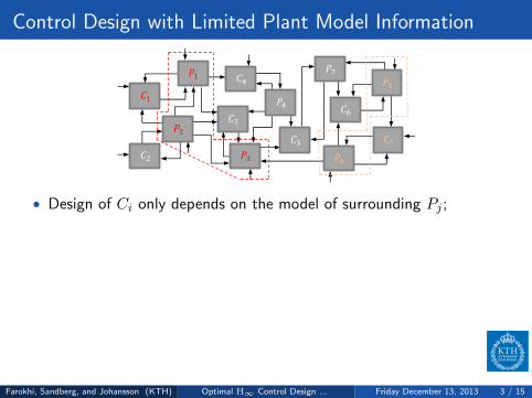
• Design of Ci only depends on the model of surrounding Pj ;
Farokhi, Sandberg, and Johansson (KTH) Optimal H∞ Control Design ... Friday December 13, 2013 3 / 15
Control Design with Limited Plant Model Information
𝐶1
𝑃1
𝑃2
𝐶4
𝐶3
𝑃3
𝑃7
𝐶5
𝐶6
𝐶2 𝑃6
𝑃5
𝐶7
𝑃4
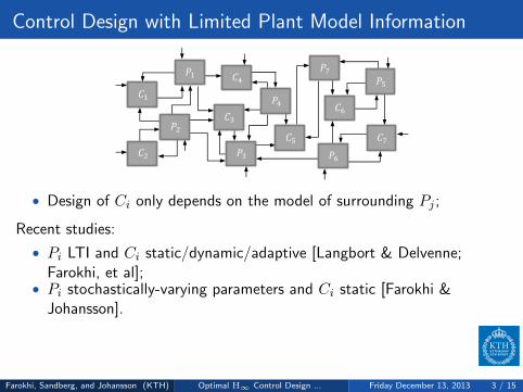
• Design of Ci only depends on the model of surrounding Pj ;
Recent studies:
• Pi LTI and Ci static/dynamic/adaptive [Langbort & Delvenne;Farokhi, et al];
• Pi stochastically-varying parameters and Ci static [Farokhi &Johansson].
Farokhi, Sandberg, and Johansson (KTH) Optimal H∞ Control Design ... Friday December 13, 2013 3 / 15
Control Design with Limited Plant Model Information
𝐶1
𝑃1
𝑃2
𝐶4
𝐶3
𝑃3
𝑃7
𝐶5
𝐶6
𝐶2 𝑃6
𝑃5
𝐶7
𝑃4
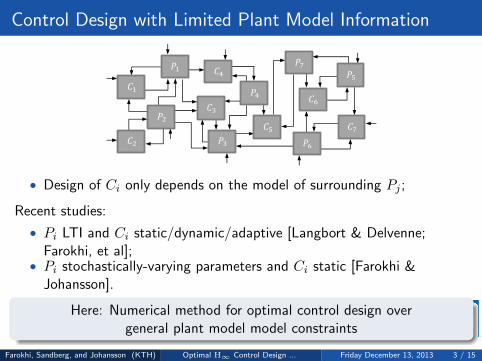
• Design of Ci only depends on the model of surrounding Pj ;
Recent studies:
• Pi LTI and Ci static/dynamic/adaptive [Langbort & Delvenne;Farokhi, et al];
• Pi stochastically-varying parameters and Ci static [Farokhi &Johansson].
Here: Numerical method for optimal control design overgeneral plant model model constraints
Farokhi, Sandberg, and Johansson (KTH) Optimal H∞ Control Design ... Friday December 13, 2013 3 / 15

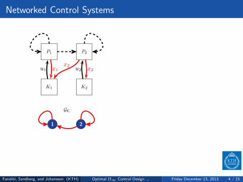
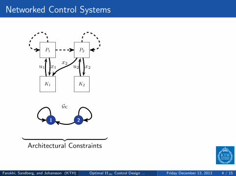
Networked Control Systems
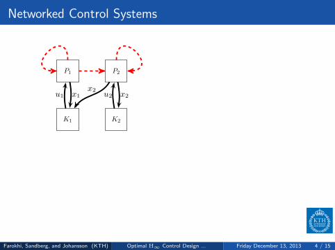
P1 P2
K1 K2
x2x1u1 x2u2
P1
GK
P2
︸ ︷︷ ︸Architectural Constraints
1
GC
2
︸ ︷︷ ︸Model Information Constraints
Farokhi, Sandberg, and Johansson (KTH) Optimal H∞ Control Design ... Friday December 13, 2013 4 / 15
Networked Control Systems
P1 P2
K1 K2
x2x1u1 x2u2
P1
GK
P2
︸ ︷︷ ︸Architectural Constraints
1
GC
2
︸ ︷︷ ︸Model Information Constraints
Farokhi, Sandberg, and Johansson (KTH) Optimal H∞ Control Design ... Friday December 13, 2013 4 / 15
Networked Control Systems
P1 P2
K1 K2
x2x1u1 x2u2
1
GK
2
︸ ︷︷ ︸Architectural Constraints
1
GC
2
︸ ︷︷ ︸Model Information Constraints
Farokhi, Sandberg, and Johansson (KTH) Optimal H∞ Control Design ... Friday December 13, 2013 4 / 15
Networked Control Systems
P1 P2
K1 K2
x2x1u1 x2u2
1
GK
2
︸ ︷︷ ︸Architectural Constraints
1
GC
2
︸ ︷︷ ︸Model Information Constraints
Farokhi, Sandberg, and Johansson (KTH) Optimal H∞ Control Design ... Friday December 13, 2013 4 / 15

Networked Control Systems
P1 P2
K1 K2
x2x1u1 x2u2
1
GK
2
︸ ︷︷ ︸Architectural Constraints
1
GC
2
︸ ︷︷ ︸Model Information Constraints
Farokhi, Sandberg, and Johansson (KTH) Optimal H∞ Control Design ... Friday December 13, 2013 4 / 15
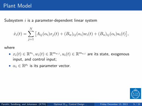
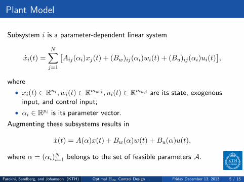
Plant Model
Subsystem i is a parameter-dependent linear system
xi(t) =
N∑j=1
[Aij(αi)xj(t) + (Bw)ij(αi)wi(t) + (Bu)ij(αi)ui(t)
],
where
• xi(t) ∈ Rni , wi(t) ∈ Rmw,i , ui(t) ∈ Rmu,i are its state, exogenousinput, and control input;
• αi ∈ Rpi is its parameter vector.
Augmenting these subsystems results in
x(t) = A(α)x(t) +Bw(α)w(t) +Bu(α)u(t),
where α = (αi)Ni=1 belongs to the set of feasible parameters A.
Farokhi, Sandberg, and Johansson (KTH) Optimal H∞ Control Design ... Friday December 13, 2013 5 / 15

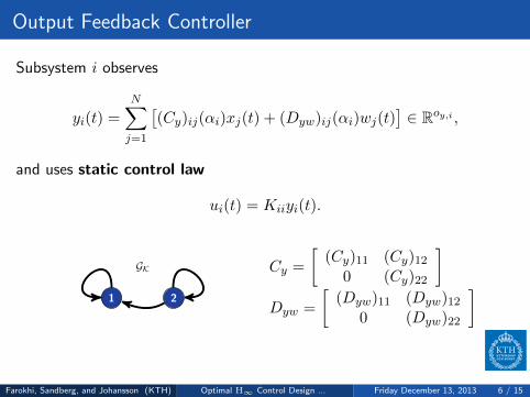
Output Feedback Controller
Subsystem i observes
yi(t) =
N∑j=1
[(Cy)ij(αi)xj(t) + (Dyw)ij(αi)wj(t)
]∈ Roy,i ,
and uses static control law
ui(t) = Kiiyi(t).
Cy =
[(Cy)11 (Cy)12
0 (Cy)22
]1
GK
2Dyw =
[(Dyw)11 (Dyw)12
0 (Dyw)22
]
Farokhi, Sandberg, and Johansson (KTH) Optimal H∞ Control Design ... Friday December 13, 2013 6 / 15
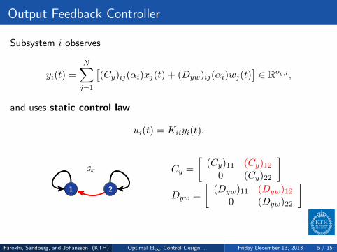

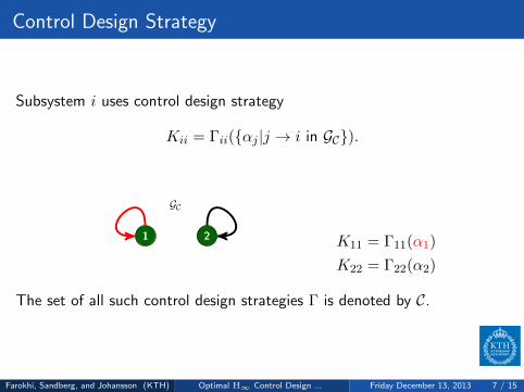
Control Design Strategy
Subsystem i uses control design strategy
Kii = Γii({αj |j → i in GC}).
1
GC
2 K11 = Γ11(α1)
K22 = Γ22(α2)
The set of all such control design strategies Γ is denoted by C.
Farokhi, Sandberg, and Johansson (KTH) Optimal H∞ Control Design ... Friday December 13, 2013 7 / 15
Control Design Strategy
Subsystem i uses control design strategy
Kii = Γii({αj |j → i in GC}).
1
GC
2 K11 = Γ11(α1)
K22 = Γ22(α2)
The set of all such control design strategies Γ is denoted by C.
Farokhi, Sandberg, and Johansson (KTH) Optimal H∞ Control Design ... Friday December 13, 2013 7 / 15
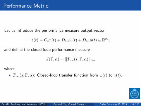
Performance Metric
Let us introduce the performance measure output vector
z(t) = Czx(t) +Dzww(t) +Dzuu(t) ∈ Roz ,
and define the closed-loop performance measure
J(Γ, α) = ‖Tzw(s; Γ, α)‖∞,
where
• Tzw(s; Γ, α): Closed-loop transfer function from w(t) to z(t).
Farokhi, Sandberg, and Johansson (KTH) Optimal H∞ Control Design ... Friday December 13, 2013 8 / 15

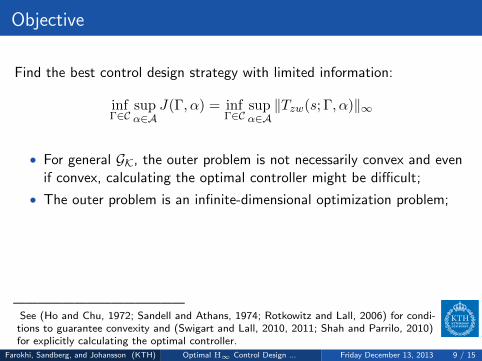
Objective
Find the best control design strategy with limited information:
infΓ∈C
supα∈A
J(Γ, α) = infΓ∈C
supα∈A‖Tzw(s; Γ, α)‖∞
——————————————See (Ho and Chu, 1972; Sandell and Athans, 1974; Rotkowitz and Lall, 2006) for condi-tions to guarantee convexity and (Swigart and Lall, 2010, 2011; Shah and Parrilo, 2010)for explicitly calculating the optimal controller.
Farokhi, Sandberg, and Johansson (KTH) Optimal H∞ Control Design ... Friday December 13, 2013 9 / 15
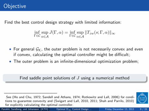
Objective
Find the best control design strategy with limited information:
infΓ∈C
supα∈A
J(Γ, α) = infΓ∈C
supα∈A‖Tzw(s; Γ, α)‖∞
• For general GK, the outer problem is not necessarily convex and evenif convex, calculating the optimal controller might be difficult;
• The outer problem is an infinite-dimensional optimization problem;
——————————————See (Ho and Chu, 1972; Sandell and Athans, 1974; Rotkowitz and Lall, 2006) for condi-tions to guarantee convexity and (Swigart and Lall, 2010, 2011; Shah and Parrilo, 2010)for explicitly calculating the optimal controller.
Farokhi, Sandberg, and Johansson (KTH) Optimal H∞ Control Design ... Friday December 13, 2013 9 / 15
Objective
Find the best control design strategy with limited information:
infΓ∈C
supα∈A
J(Γ, α) = infΓ∈C
supα∈A‖Tzw(s; Γ, α)‖∞
• For general GK, the outer problem is not necessarily convex and evenif convex, calculating the optimal controller might be difficult;
• The outer problem is an infinite-dimensional optimization problem;
Find saddle point solutions of J using a numerical method
——————————————See (Ho and Chu, 1972; Sandell and Athans, 1974; Rotkowitz and Lall, 2006) for condi-tions to guarantee convexity and (Swigart and Lall, 2010, 2011; Shah and Parrilo, 2010)for explicitly calculating the optimal controller.
Farokhi, Sandberg, and Johansson (KTH) Optimal H∞ Control Design ... Friday December 13, 2013 9 / 15
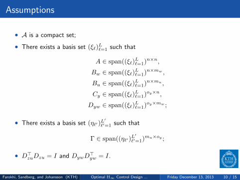
Assumptions
• A is a compact set;
• There exists a basis set (ξ`)L`=1 such that
A ∈ span((ξ`)L`=1)n×n,
Bw ∈ span((ξ`)L`=1)n×mw ,
Bu ∈ span((ξ`)L`=1)n×mu ,
Cy ∈ span((ξ`)L`=1)oy×n,
Dyw ∈ span((ξ`)L`=1)oy×mw ;
• There exists a basis set (η`′)L′
`′=1 such that
Γ ∈ span((η`′)L′
`′=1)mu×oy ;
• D>zuDzu = I and DywD>yw = I.
Farokhi, Sandberg, and Johansson (KTH) Optimal H∞ Control Design ... Friday December 13, 2013 10 / 15
Saddle Point Solution
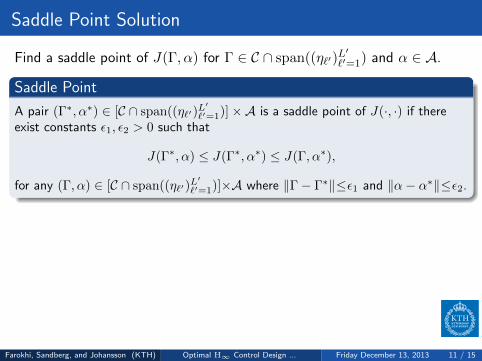
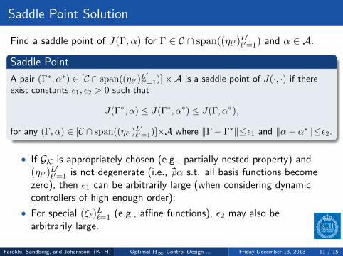
Find a saddle point of J(Γ, α) for Γ ∈ C ∩ span((η`′)L′`′=1) and α ∈ A.
Saddle Point
A pair (Γ∗, α∗) ∈ [C ∩ span((η`′)L′
`′=1)]×A is a saddle point of J(·, ·) if thereexist constants ε1, ε2 > 0 such that
J(Γ∗, α) ≤ J(Γ∗, α∗) ≤ J(Γ, α∗),
for any (Γ, α) ∈ [C ∩ span((η`′)L′
`′=1)]×A where ‖Γ− Γ∗‖≤ε1 and ‖α− α∗‖≤ε2.
• If GK is appropriately chosen (e.g., partially nested property) and(η`′)
L′`′=1 is not degenerate (i.e., @α s.t. all basis functions become
zero), then ε1 can be arbitrarily large (when considering dynamiccontrollers of high enough order);
• For special (ξ`)L`=1 (e.g., affine functions), ε2 may also be
arbitrarily large.
Farokhi, Sandberg, and Johansson (KTH) Optimal H∞ Control Design ... Friday December 13, 2013 11 / 15
Saddle Point Solution
Find a saddle point of J(Γ, α) for Γ ∈ C ∩ span((η`′)L′`′=1) and α ∈ A.
Saddle Point
A pair (Γ∗, α∗) ∈ [C ∩ span((η`′)L′
`′=1)]×A is a saddle point of J(·, ·) if thereexist constants ε1, ε2 > 0 such that
J(Γ∗, α) ≤ J(Γ∗, α∗) ≤ J(Γ, α∗),
for any (Γ, α) ∈ [C ∩ span((η`′)L′
`′=1)]×A where ‖Γ− Γ∗‖≤ε1 and ‖α− α∗‖≤ε2.
• If GK is appropriately chosen (e.g., partially nested property) and(η`′)
L′`′=1 is not degenerate (i.e., @α s.t. all basis functions become
zero), then ε1 can be arbitrarily large (when considering dynamiccontrollers of high enough order);
• For special (ξ`)L`=1 (e.g., affine functions), ε2 may also be
arbitrarily large.
Farokhi, Sandberg, and Johansson (KTH) Optimal H∞ Control Design ... Friday December 13, 2013 11 / 15
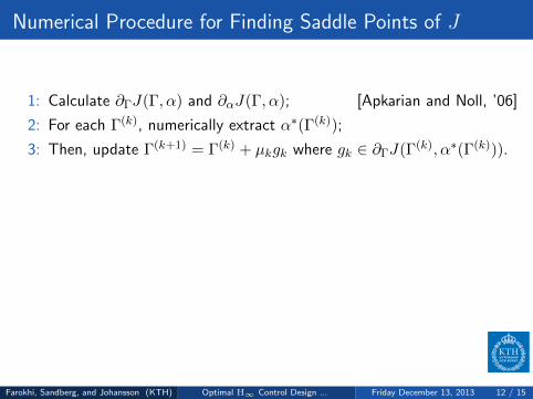
Numerical Procedure for Finding Saddle Points of J
1: Calculate ∂ΓJ(Γ, α) and ∂αJ(Γ, α); [Apkarian and Noll, ’06]
2: For each Γ(k), numerically extract α∗(Γ(k));
3: Then, update Γ(k+1) = Γ(k) + µkgk where gk ∈ ∂ΓJ(Γ(k), α∗(Γ(k))).
Theorem
Let {µk}∞k=0 be chosen such that limk→∞∑k
z=1 µz =∞ and
limk→∞∑k
z=1 µ2z <∞. Assume that the subgradients are uniformly
bounded for all iterations. If the numerical procedure converges, it gives asaddle point of J .
Farokhi, Sandberg, and Johansson (KTH) Optimal H∞ Control Design ... Friday December 13, 2013 12 / 15
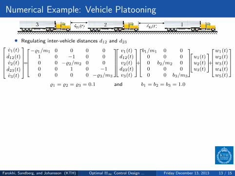
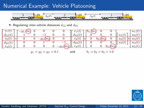
Numerical Example: Vehicle Platooning
• Regulating inter-vehicle distances d12 and d23v1(t)
d12(t)v2(t)
d23(t)v3(t)
=−%1/m1 0 0 0 0
1 0 −1 0 00 0 −%2/m2 0 00 0 1 0 −10 0 0 0 −%3/m3
v1(t)d12(t)v2(t)d23(t)v3(t)
+b1/m1 0 0
0 0 00 b2/m2 00 0 00 0 b3/m3
u1(t)u2(t)u3(t)
+w1(t)w2(t)w3(t)w4(t)w5(t)
%1 = %2 = %3 = 0.1 and b1 = b2 = b3 = 1.0
1
GK
2
3
Farokhi, Sandberg, and Johansson (KTH) Optimal H∞ Control Design ... Friday December 13, 2013 13 / 15

Numerical Example: Vehicle Platooning
• Regulating inter-vehicle distances d12 and d23v1(t)
d12(t)v2(t)
d23(t)v3(t)
=−%1/m1 0 0 0 0
1 0 −1 0 00 0 −%2/m2 0 00 0 1 0 −10 0 0 0 −%3/m3
v1(t)d12(t)v2(t)d23(t)v3(t)
+b1/m1 0 0
0 0 00 b2/m2 00 0 00 0 b3/m3
u1(t)u2(t)u3(t)
+w1(t)w2(t)w3(t)w4(t)w5(t)
z(t) =
[d12(t) d23(t) u1(t) u2(t) u3(t)
]>• Find a saddle point of J(Γ, α) = ‖Tzw (s; Γ, α)‖∞ when α = [m1m2m3]> ∈ [0.5, 1.0]3
and Γ belongs to the set of polynomials of αi, i = 1, 2, 3, up to the second order.
1
GK
2
3
Farokhi, Sandberg, and Johansson (KTH) Optimal H∞ Control Design ... Friday December 13, 2013 13 / 15
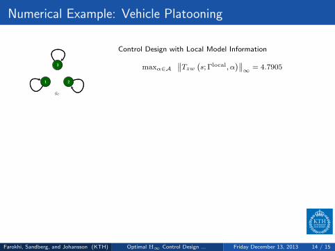
Numerical Example: Vehicle Platooning
1
GC
2
3
Control Design with Local Model Information
maxα∈A∥∥Tzw (s; Γlocal, α
)∥∥∞ = 4.7905
1
GC
2
3
Control Design with Limited Model Information
maxα∈A∥∥Tzw (s; Γlimited, α
)∥∥∞ = 3.5533
1
GC
2
3
Control Design with Full Model Information
maxα∈A∥∥Tzw (s; Γfull, α
)∥∥∞ = 3.3596
Farokhi, Sandberg, and Johansson (KTH) Optimal H∞ Control Design ... Friday December 13, 2013 14 / 15
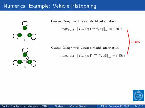
Numerical Example: Vehicle Platooning
25.8%
1
GC
2
3
Control Design with Local Model Information
maxα∈A∥∥Tzw (s; Γlocal, α
)∥∥∞ = 4.7905
1
GC
2
3
Control Design with Limited Model Information
maxα∈A∥∥Tzw (s; Γlimited, α
)∥∥∞ = 3.5533
1
GC
2
3
Control Design with Full Model Information
maxα∈A∥∥Tzw (s; Γfull, α
)∥∥∞ = 3.3596
Farokhi, Sandberg, and Johansson (KTH) Optimal H∞ Control Design ... Friday December 13, 2013 14 / 15

Numerical Example: Vehicle Platooning
25.8%
5.4%
1
GC
2
3
Control Design with Local Model Information
maxα∈A∥∥Tzw (s; Γlocal, α
)∥∥∞ = 4.7905
1
GC
2
3
Control Design with Limited Model Information
maxα∈A∥∥Tzw (s; Γlimited, α
)∥∥∞ = 3.5533
1
GC
2
3
Control Design with Full Model Information
maxα∈A∥∥Tzw (s; Γfull, α
)∥∥∞ = 3.3596
Farokhi, Sandberg, and Johansson (KTH) Optimal H∞ Control Design ... Friday December 13, 2013 14 / 15

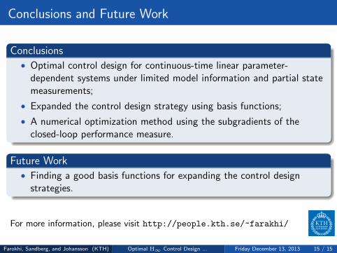
Conclusions and Future Work
Conclusions• Optimal control design for continuous-time linear parameter-
dependent systems under limited model information and partial statemeasurements;
• Expanded the control design strategy using basis functions;
• A numerical optimization method using the subgradients of theclosed-loop performance measure.
Future Work• Finding a good basis functions for expanding the control design
strategies.
For more information, please visit http://people.kth.se/~farakhi/
Farokhi, Sandberg, and Johansson (KTH) Optimal H∞ Control Design ... Friday December 13, 2013 15 / 15


![CALOREE: Learning Control for Predictable Latency and Low Energyhankhoffmann/caloree.pdf · 2018. 1. 23. · Netlix algorithm[3, 12]Ðand a hierarchical Bayesian model 1Control And](https://img.pdfslide.net/doc/110x75/6122b7313b86c272f9625409/caloree-learning-control-for-predictable-latency-and-low-energy-hankhoffmanncaloreepdf.jpg)