Embed Size (px)
Citation preview

Optimal Implementation of Simulink Models on Multicore
Architectures with Partitioned Fixed Priority Scheduling
Shamit Bansal
Thesis submitted to the Faculty of the
Virginia Polytechnic Institute and State University
in partial fulfillment of the requirements for the degree of
Masters of Science
in
Computer Engineering
Haibo Zeng, Chair
Patrick R. Schaumont
Cameron D. Patterson
April 27, 2018
Blacksburg, Virginia
Keywords: Simulink, Multicore, Software Synthesis, Partitioned scheduling
Copyright 2018, Shamit Bansal
Optimal Implementation of Simulink Models on Multicore
Architectures with Partitioned Fixed Priority Scheduling
Shamit Bansal
(ABSTRACT)
Model-based design based on the Simulink modeling formalism and the associated toolchain
has gained its popularity in the development of complex embedded control systems. How-
ever, the current research on software synthesis for Simulink models has a critical gap for
providing a deterministic, semantics-preserving implementation on multicore architectures
with partitioned fixed-priority scheduling. In this thesis, we propose to judiciously assign
task offset, task priority, and task communication mechanism, to avoid simultaneous access
to shared memory by tasks on different cores, to preserve the model semantics, and to opti-
mize the control performance. We develop two approaches to solve the problem: (a) a mixed
integer linear programming (MILP) formulation; and (b) a problem specific exact algorithm
that may run several magnitudes faster than MILP.

Optimal Implementation of Simulink Models on Multicore
Architectures with Partitioned Fixed Priority Scheduling
Shamit Bansal
(GENERAL AUDIENCE ABSTRACT)
To save development time and money, automotive industries have been developing models
using software, before implementing them directly on hardware. For reliability, the model
generated from the software tool should behave in a well defined manner, coherent to the
ideal design of the model. While the current tools are able to generate this reliable model for
a single processor system, they are not able to do so for a system with multiple processors.
When two or more processors contend to access the same resource at the same time, the
existing tools are unable to provide a well defined execution order in their model. Since
modern embedded systems need multiple processors to meet their increasing performance
demands, it is imperative that the software tools scale up to multiple processors as well. In
this work, we seek to bridge this gap by presenting two solutions that generate a deterministic
software implementation of a system with multiple processors. In our solutions, we generate
a model with well defined execution order by ensuring that at any given time, only one
processor accesses a given resource. Furthermore, apart from ensuring determinism, we also
improve upon the performance of the generated model by ensuring that there is minimal
end-to-end latency in the system.

Dedication
Dedicated to my parents
iv

Acknowledgments
First and foremost, I wish to thank my advisor Dr. Haibo Zeng for his guidance throughout
my masters. His consistent support and sound advice during the course of this research will
remain as a solid foundation in my future professional career. I am grateful to him for always
steering me in the right direction with his innovative ideas, great knowledge and experience.
In the past year, he has not only helped me grow as a researcher but also as a professional
with his mentorship. Lastly, I wish to thank him for being so patient with me, as without
his support this thesis would not have been possible. I wish to thank the experts on my
review committee Dr. Cameron Patterson and Dr. Patrick Schaumont for taking time out
of their busy schedule to read this thesis and providing valuable feedback. I also wish to
thank them for teaching me two of the best courses I have had the opportunity to attend at
Virginia Tech. I am grateful to Yecheng Zhao for all his help during the course of this project.
Being new to this domain, I was easily overwhelmed and confused in the beginning. But
he patiently handled all my doubts and helped me understand the fundamental concepts
of software programming as well as real-time systems. I will forever be indebted to my
family back home for being the constant source of encouragement and support in my life. I
wish to thank my labmate Prachi Joshi for being so helpful and providing valuable tips and
suggestions on writing this thesis. I am thankful to my friend in Michigan, Uthara Menon
for her support, motivation and advice on life in general. I would also like to thank all my
friends in Blacksburg: Vamsi, Aarushi, Omkar, Tania, Kunal, Surabhi, Abhishek, Manish,
Shruti, Akshay and Vibhav who made the last two years, the best years of my life. Last but
not the least, I thank my childhood friend Shubham Sarin for always encouraging me and
helping me stay confident and positive.
v

Contents
List of Figures ix
List of Tables xi
1 Introduction 1
1.1 Synchronous Reactive Models . . . . . . . . . . . . . . . . . . . . . . . . . . 3
1.2 Software Synthesis of SR models . . . . . . . . . . . . . . . . . . . . . . . . . 4
1.3 Our Contribution . . . . . . . . . . . . . . . . . . . . . . . . . . . . . . . . . 7
1.4 Organization . . . . . . . . . . . . . . . . . . . . . . . . . . . . . . . . . . . 9
2 Related Work 10
3 Mechanisms for Preserving Communication Semantics 14
3.1 Preliminary . . . . . . . . . . . . . . . . . . . . . . . . . . . . . . . . . . . . 14
3.1.1 Semantics For Communication . . . . . . . . . . . . . . . . . . . . . . 15
3.1.2 Challenges to Preserving Semantics . . . . . . . . . . . . . . . . . . . 19
3.1.3 Preserving Semantics on Single-core . . . . . . . . . . . . . . . . . . . 22
3.2 Task Model for Multicore Architecture . . . . . . . . . . . . . . . . . . . . . 26
3.3 Preserving Semantics on Multicore Architecture . . . . . . . . . . . . . . . . 28
vi

3.3.1 Preserving Intra-core Communication Semantics . . . . . . . . . . . . 28
3.3.2 Inter-core Communication Semantics . . . . . . . . . . . . . . . . . . 31
4 Problem Formulation 35
5 MILP Formulation 37
6 Customized Optimization Algorithm 43
6.1 Problem Formulation for MIXO Framework . . . . . . . . . . . . . . . . . . 47
6.2 MIXO Computation . . . . . . . . . . . . . . . . . . . . . . . . . . . . . . . 49
6.3 Feasibility Analysis for MIXO Based Framework . . . . . . . . . . . . . . . . 50
6.3.1 Exact Feasibility Analysis . . . . . . . . . . . . . . . . . . . . . . . . 51
6.3.2 Necessary Feasibility Analysis 1 . . . . . . . . . . . . . . . . . . . . . 54
6.3.3 Necessary Feasibility Analysis 2 . . . . . . . . . . . . . . . . . . . . . 58
6.3.4 Final Algorithm for Feasibility Analysis . . . . . . . . . . . . . . . . 59
6.4 MILP for MIXO Based Framework . . . . . . . . . . . . . . . . . . . . . . . 61
6.5 Putting All Together - MIXO-Guided Framework . . . . . . . . . . . . . . . 61
7 Results 66
7.1 Experiment on Random Systems . . . . . . . . . . . . . . . . . . . . . . . . 66
7.2 Fuel Injection System Case Study . . . . . . . . . . . . . . . . . . . . . . . . 70
8 Conclusion and Future Work 72
vii

Bibliography 73
viii

List of Figures
1.1 Determinism in concurrent SR Models, such that black arrow represents trig-
ger of task, dotted line represents global tick and the blue arrow represents
data flow . . . . . . . . . . . . . . . . . . . . . . . . . . . . . . . . . . . . . . 3
1.2 Deterministic Execution Order in single-core, such that black arrow represents
trigger of task and dotted line represents global tick . . . . . . . . . . . . . . 5
1.3 Deterministic Execution Order in multi-core, such that black arrow represents
trigger of task and dotted line represents global tick . . . . . . . . . . . . . . 6
3.1 Input/output relation with direct feedthrough on the communication link with
(A) TNi< TNj
(B) TNi> TNj
. . . . . . . . . . . . . . . . . . . . . . . . . . . 17
3.2 Input/output relation with unit delay on the communication link with (A)
TNi< TNj
(B) TNi> TNj
. . . . . . . . . . . . . . . . . . . . . . . . . . . . . 18
3.3 Impact of Delay on Data Integrity on directfeedthrough with (A) TNi< TNj
(B) TNi> TNj
. . . . . . . . . . . . . . . . . . . . . . . . . . . . . . . . . . . 20
3.4 Impact of Delay on Data Integrity on a link with unit delay where (A) TNi>
TNj(B) TNi
< TNj. . . . . . . . . . . . . . . . . . . . . . . . . . . . . . . . 21
3.5 Preserving Data Integrity by RT blocks for directfeedthrough in single-core
with (A) TNi< TNj
(B)TNi> TNj
. . . . . . . . . . . . . . . . . . . . . . . . 24
3.6 Preserving Data Integrity by RT blocks for unit delay link in single-core with
(A) TNi> TNj
(B) TNi< TNj
. . . . . . . . . . . . . . . . . . . . . . . . . . . 25
ix

3.7 Preserving the communication semantics for Intra-core directfeedthrough Link
with (A) TNi< TNj
(B) TNi> TNj
. . . . . . . . . . . . . . . . . . . . . . . . 30
3.8 Preserving the communication semantics for Intra-core unit-delay Link with
(A) TNi> TNj
(B) TNi< TNj
. . . . . . . . . . . . . . . . . . . . . . . . . . . 31
3.9 Preserving the communication semantics for Inter-core directfeedthrough Link
with (A) TNi< TNj
(B) TNi> TNj
. . . . . . . . . . . . . . . . . . . . . . . . 33
3.10 Preserving the communication semantics for Inter-core Link with Unit-Delay
with (A) TNi> TNj
(B) TNi< TNj
. . . . . . . . . . . . . . . . . . . . . . . . 34
6.1 High Level Overview of Proposed Framework . . . . . . . . . . . . . . . . . . 43
6.2 MUDA Framework Overview . . . . . . . . . . . . . . . . . . . . . . . . . . . 52
6.3 MIXO-guided Framework . . . . . . . . . . . . . . . . . . . . . . . . . . . . . 60
7.1 Average Run-Time for 1000 Random Systems . . . . . . . . . . . . . . . . . 67
7.2 Average Run-Time for 50 tasks vs Utilization . . . . . . . . . . . . . . . . . 68
7.3 Normalized Objective Analysis for 1000 Random systems . . . . . . . . . . . 69
x

List of Tables
5.1 Notations Used in our implementation . . . . . . . . . . . . . . . . . . . . . 38
6.1 Example Test Case . . . . . . . . . . . . . . . . . . . . . . . . . . . . . . . . 45
7.1 Comparing performance of each Analysis . . . . . . . . . . . . . . . . . . . 68
7.2 Results for 1000 Random Systems . . . . . . . . . . . . . . . . . . . . . . . . 70
7.3 Results for Fuel-Injection Case Study . . . . . . . . . . . . . . . . . . . . . . 71
xi

List of Abbreviations
DAG Directed Acyclic Graph
DF Direct Feedthrough
ILP Integer Linear Programming
LH Low rate to High rate
MBD Model Based Design
MILP Mixed Integer Linear Programming
MIXO Minimal Infeasible partial eXecution Order
MUDA Maximal Unschedulable Deadline Assignment
RT Rate Transition
SR Synchronous Reactive
UD Unit Delay
WCET Worst Case Execution Time
WCRT Worst Case Response Time
xii

Chapter 1
Introduction
With the embedded systems becoming more complex day-by-day, the traditional manual
software development is too slow and prone to errors. Thus the industries have shifted to
using a model-based design (MBD) for developing embedded software for complex systems
such as flight controllers, engine control and fuel injection systems. MBDs help shorten the
development time by providing a visual abstraction of the system and allowing easier inte-
gration for complex systems. Additionally they allow the designer to evaluate the system
performance, design trade-offs and even test the system functionality in a simulated environ-
ment. To provide maximum utility, the MBDs need to be accompanied by automatic code
generation tools that can help in providing embedded software ready for deployment.
For the automotive industry, Simulink based MBDs with their well-defined formalism and
associated toolchain have been a popular choice for a while now. For reduced implementa-
tion errors and faster turn-around times, tools such as Simulink Coder [45] are being used to
automatically generate software implementations on single-core architectures. However, due
to physical limitations the single-core architecture is reaching the limits of its computational
capability. Thus, modern automotive systems are focusing on using multicore architecture
to meet their increasing performance and efficiency demands. By allowing multiple proces-
sors to run concurrently, multicore architecture allows for a higher throughput than possible
with a single processor. This migration however, creates a gap in research as the current
solutions for semantics-preserving software implementation for Simulink models, including
1

2 Chapter 1. Introduction
those provided by the commercial code generators, do not scale to multicore architectures.
For example, the Simulink toolchain relies on users to specify the data communication mech-
anisms, and the generated coder may have non-deterministic behavior and cannot guarantee
to be semantics preserving [12].
The necessary requirement of generating a reliable software implementation is that it should
follow the semantics of the ideal model. With synchronous reactive (SR) as the underlying
formalism, simulated Simulink models assume that the tasks have atomic operation that
follow a defined causality order [41]. To implement SR models successfully for a multicore
system, the challenge is to ensure that the generated implementation of the system follows
the logical-time execution semantics. This is not a trivial problem, as in real-time implemen-
tation the blocks do not run with a zero-execution time but rather have an execution time
dependent upon the scheduling policy as well as on the interference rising from contention
for shared resource. As multiple tasks compete for the shared resources across multiple cores,
the possible thread-interleavings may further give rise to multiple possible execution orders.
Since, there is no defined execution order, the reliability of the generated software suffers by
a great deal. For safety-critical embedded systems such as a flight management system, this
non-determinism can prove to be quite fatal [20]. Furthermore, in order to ensure that the
semantics of communication are preserved, the generated system sometimes requires addi-
tion of sample-and-hold buffers. However, these buffers may further add functional delay in
the system delay blocks which adversely affects the end-to-end latency and may have critical
impacts for control-command systems such as those used in avionics [22].
Our objective in this work is to ensure that the generated deterministic software implemen-
tation for multicore Simulink models preserves the logical-time execution semantics of a SR
model while providing optimal control performance.

1.1. Synchronous Reactive Models 3
A100 Hz
B50 Hz
Time
A A A A
Time
B B
Core 1
Core 0
Figure 1.1: Determinism in concurrent SR Models, such that black arrow represents triggerof task, dotted line represents global tick and the blue arrow represents data flow
1.1 Synchronous Reactive Models
SR models can be viewed as logically timed models similar to the cycle-based systems present
in hardware designs, where the concurrent actions of the system are associated with each
tick of the global clock. This type of model ensures that for the same set of inputs, we get
the same set of outputs at every tick. Since these models consider atomic operations, they
do not allow multiple possible interleavings, thus providing a deterministic execution order
in the system. This atomic operation can be seen in Figure 1.1, as A (producing output at
100 Hz) and B (producing output at 50 Hz) are triggered at the same time and B obtains the
data from the most recent instance of A. The communication flow of the data represented
by blue arrow shows this operation while assuming logical-time execution semantics. Since
SR models assume atomic operation with negligible execution time, there is no data race
condition and hence deterministic data transfer is ensured. The precision provided by SR
models has further propagated its use in widespread industrial applications. Currently SR is
the underlying modeling formalism for various languages such as Esterel[6], Lustre [24] and

4 Chapter 1. Introduction
the Simulink graphical language[45]. The formal properties that these languages allow for
an easier validation and verification of the generated model. For example, SCADE (Safety
Critical Application Development Environment) is an industrial application of Lustre which
is used in design of safety-critical flight controller software systems, engine control systems,
automatic pilot systems, etc.
Thus if generated correctly, the software implementation based on SR formalism will always
provide a deterministic execution order which is essential for any reliable implementation. In
the following subsection, we briefly explain how we ensure that our generated model follows
the logical-time execution semantics of the SR model for multicore systems.
1.2 Software Synthesis of SR models
When synthesizing software implementation of Simulink models, the generated implementa-
tion should preserve the semantics of the ideal model mentioned above. This is challenging
as in real-time implementation the blocks do not run with a zero-execution time but rather
have an execution time dependent upon the scheduling policy as well as on the interference
rising from contention for shared resource. To ensure that the semantics of simulated model
(as shown in Figure 1.1) are preserved in the generated single-core model, Simulink adds
Rate Transition (RT) blocks as a form of wait-free buffer [45] between two communicating
tasks (as shown in Figure 1.2). These blocks are required for ensuring data integrity as well
deterministic transfer of data between tasks running at different rates [12, 50] (see Section
3.1.3). For a single-core architecture, using RT blocks with a defined priority assignment
allows the generated software implementation to follow a deterministic execution order as
shown in Figure 1.2. We see that by assigning A a higher priority than B and using RT block
to buffer A’s output, we can ensure the communication semantics of simulated model in Fig-
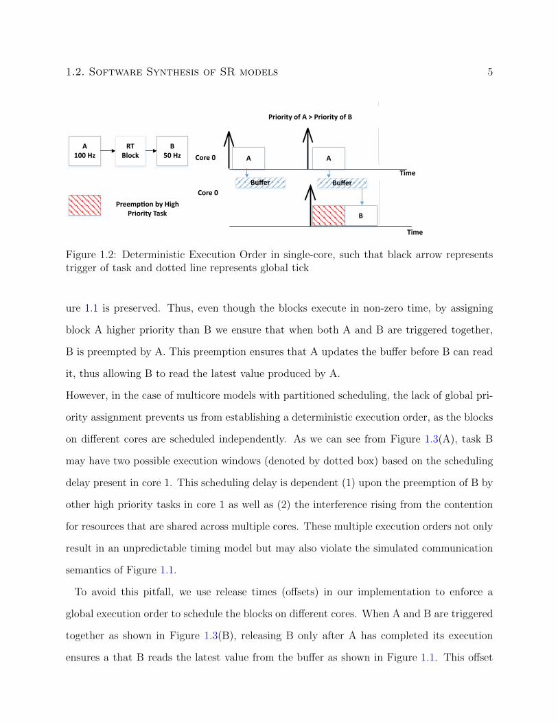
1.2. Software Synthesis of SR models 5
Time
Time
A100 Hz
B50 Hz ACore 0
B
Priority of A > Priority of B
Core 0
A
RT Block
Buffer
Preemp�on by High Priority Task
Buffer
Figure 1.2: Deterministic Execution Order in single-core, such that black arrow representstrigger of task and dotted line represents global tick
ure 1.1 is preserved. Thus, even though the blocks execute in non-zero time, by assigning
block A higher priority than B we ensure that when both A and B are triggered together,
B is preempted by A. This preemption ensures that A updates the buffer before B can read
it, thus allowing B to read the latest value produced by A.
However, in the case of multicore models with partitioned scheduling, the lack of global pri-
ority assignment prevents us from establishing a deterministic execution order, as the blocks
on different cores are scheduled independently. As we can see from Figure 1.3(A), task B
may have two possible execution windows (denoted by dotted box) based on the scheduling
delay present in core 1. This scheduling delay is dependent (1) upon the preemption of B by
other high priority tasks in core 1 as well as (2) the interference rising from the contention
for resources that are shared across multiple cores. These multiple execution orders not only
result in an unpredictable timing model but may also violate the simulated communication
semantics of Figure 1.1.
To avoid this pitfall, we use release times (offsets) in our implementation to enforce a
global execution order to schedule the blocks on different cores. When A and B are triggered
together as shown in Figure 1.3(B), releasing B only after A has completed its execution
ensures a that B reads the latest value from the buffer as shown in Figure 1.1. This offset

6 Chapter 1. Introduction
Time
Time
A100 Hz
B50 Hz ACore 0
B
Core 1
A
RT Block
BufferBuffer
B
Time
Time
A
B
A
BufferBuffer
Offset For B
Core 1
Core 0
A)
B)
Figure 1.3: Deterministic Execution Order in multi-core, such that black arrow representstrigger of task and dotted line represents global tick
assignment ensures that a deterministic execution order is followed while ensuring data in-
tegrity. Furthermore, we also use this offset assignment to separate the execution windows of
tasks that seek to access the same resource. Thus we need to ensure that when A is accessing
the buffer, B should not be executing. In order to do so, we release B only when A is done
with its execution and the buffer is free. This temporal isolation between communicating
tasks further helps in timing predictability as now software on different cores does not access
the same resource at the same time.
Combining separate execution windows with wait-free RT blocks will now allow the writer
to write its data into a buffer and the reader to independently read from the given buffer
index during its execution. This ensures data consistency and semantics preservation of
the simulated model as shown in Figure 1.1. However, if the reader is unable to meet its

1.3. Our Contribution 7
deadline, the addition of this RT block sometimes requires using sample-and-hold operation
to ensure data integrity (described in section 3.1.3). This sample-and-hold operation adds
functional delay in the system by relaxing the input/output dependency within the same
cycle (tick). While this relaxed dependency improves schedulability (see section 3.1.1), it
can cause control performance degradation and even system instability [18].
The optimal software synthesis of multicore Simulink models can be formalized as the fol-
lowing design optimization problem: finding a deterministic implementation that follows the
semantics of the ideal model and requires the addition of the minimum number of functional
delays to do so. For this deterministic implementation, we need to ensure that all the tasks
meet their respective deadlines (i.e. within each tick) while following the causality order of
the simulated model. To solve this optimization problem, we briefly discuss our contribution
in the following sub-section.
1.3 Our Contribution
In our work, we consider partitioned fix-priority scheduling due to its extensive use in indus-
trial standards such as AUTOmotive Open Source ARchitecture (AUTOSAR), commercial
real time operating systems such as VxWorks, and in particular, the code generators for
Simulink such as Embedded Coder. Partitioned scheduling essentially means that no notion
of global priority exists and the tasks cannot migrate between cores. Since there is no notion
of global priority across cores, in order to ensure the deterministic implementation, we need
to solve the system for the following
• assignment of release time of each task to ensure separate execution windows and
establishing an execution order across all the cores

8 Chapter 1. Introduction
• assignment of priorities to tasks on the same core, such that the tasks meet their
deadlines and enforce an execution order within the core
• assignment of the communication mechanism i.e. addition of functional delays using
sample-and-hold buffers, on communication links if required for preservation of com-
munication semantics
The objective of our optimization problem is to find a deterministic implementation with
minimal cost in terms of added delays for a given multicore system. In our analysis, we
assume that the allocation of tasks to cores is already provided to us and leave the optimal
partitioning scheme as future work.
In this thesis we provide two approaches to solve the optimal software synthesis problem.
In the first approach we develop a Mixed Integer Linear Programming (MILP) formulation
for the problem (see Chapter 5) that defines the model in terms of mathematical constraints
and then searches for the optimal solution. Second, we develop a problem specific framework
that starts with zero delay block assignment initially and then adds delay block to a link
only if it is necessary for schedulability (see Chapter 6). The obtained results (see Section
7.1) show that our proposed framework is more scalable than the standard MILP while
preserving the optimality of the solution, thus making it a suitable alternative for finding an
optimal solution for medium and large sized systems.
For evaluating the performance of both the approaches, we perform our experiments on
an industrial case study as well as on randomly generated systems. By evaluating the
performance on a simplified version of the fuel injection systems [17], we show how efficient
our proposed framework is when it comes to handling a real-world problem. The results from
the case study show that our approach performs 2-3 orders of magnitude faster than the
MILP while preserving the optimality of the solution.

1.4. Organization 9
1.4 Organization
In this thesis, we organize the contents as following :
1. Chapter 2 discusses related work in this domain.
2. Chapter 3 discusses the semantics of the communication and the mechanisms used for
preservation of the communication semantics.
3. Chapter 4 formally defines the optimization problem that we seek to solve.
4. Chapter 5 talks about the MILP formulation used to solve the defined optimization
problem
5. Chapter 6 explains the problem specific exact algorithm that outperforms MILP
6. Chapter 7 discusses the results that we get from experiments on random systems as
well as from the industrial case study for both the approaches
7. Chapter 8 provides the conclusion of this work along with future work that can be
incorporated in this problem
Conference
The following is the conference to which this work has been submitted
• Bansal S., Zhao Y., Zeng H., Yang K. “Optimal Implementation of Simulink Models
on Multicore Architectures with Partitioned Fixed Priority Scheduling”, International
Conference on Embedded Software (EMSOFT). Submitted.
Chapter 2
Related Work
To provide a deterministic timing predictable model for multicore embedded systems, the
interference from contention for shared resources has to be considered to estimate the execu-
tion time of each task [40]. A survey of this interference and its effect on response time has
been done by Axer et al. [5], Wegener [48]. While computing the response time for multicore
system is not our objective, it is relevant to discuss the common approaches that have been
used to deal with the interference that rises when software on different cores access the same
resource. The said approaches can be broadly divided into two categories as shown below:
. Computing the impact of the interferences and adding them to analysis[3], [33]. Alt-
meyer et al. [3] in their work, provide a general framework used that analyzes the individual
interferences on bus, memory as well as on the core to compute the net impact of interfer-
ence on the response time. Rihani et al. [44] in their work build upon the generic framework
developed in [3] to compute the impact of interference specifically for synchronous data flow
graphs. Davis et al. [15] consider the memory demand and processor demand of each task
and hence use it to compute the interference caused by the execution of a given task on the
system, thus providing a more exact solution than [3]. Kang et al. [26] in their work compute
the interference that rises from all 4 possible types of communication i.e. high priority to low
priority on same core and different core as well as low priority to high priority on same core
and different core. Our approach may be considered complimentary to all these approaches
as we seek to minimize this interference for deterministic execution. Similar to our approach,
10

11
Martinez et al. [32] in their work also develop a technique to reduce the contention by using
slack-time and hence work with framework of [44] to show that reduced contention improves
the performance. However, their work is not scalable and they left the optimization as future
work. Kelter and Marwedel [27] analyze all possible paths of execution for a given task and
thus provide the worst-case execution order. However, this technique is also not scalable to
large systems and is currently implemented only for a single rate system with non preemptive
execution, thus limiting its application. Thus we see that in order to obtain a deterministic
execution order and save ourselves from state explosion, we need to mitigate the interference
completely as shown below.
. Mitigating the effects of such interferences by techniques such as temporal isolation
[7] or resource partitioning [37]. The objective of this approach is to reduce the cost of inter-
ference on analysis of deterministic execution. Perret et al. [37] discuss how spatial isolation
of resources and temporal isolation for execution (Time Division Multiplexed Arbitration for
accessing the bus) can help in obtaining a deterministic multicore model. Maia et al. [30]
provide this robust partitioning of resources by using isolated windows of execution for each
task. Thus the execution of a task cannot have any impact on the execution of any other
task. A real life application of these techniques have been presented in [20]. Durrieu et al.
[20] have successfully developed a deterministic flight management system by using these iso-
lated execution windows of the tasks. However, to manage the intra-core interference they
impose non-preemptive scheduling whereas we account for that interference as well in our
analysis. The work done by Carle et al. [8] also uses temporal isolation between dependent
tasks to provide a deterministic multi core system. However, their schedulability analysis
does not scale well and has a 1 hour-timeout rate for 50% cases at 50 tasks itself. Klikpo
and Munier-Kordon [28] in their work develop a heuristic that uses temporal isolation for
providing deterministic execution for a synchronous data flow graph. However, their work

12 Chapter 2. Related Work
provides a sub-optimal solution and works only on a uniprocessor system. As mentioned in
[34], synchronization of dependent tasks also has a cost on response time analysis. However,
our approach successfully avoids this cost by using temporal isolation of dependent tasks,
thus turning them into independent tasks.
Although our focus is on Simulink model, we discuss the related work in the broader con-
text of Synchronous reactive (SR) model of computation, as it is the underlying modeling
formalism for Simulink [45]. SR is supported in several other languages such as Esterel [6],
Lustre [24], and Prelude [21, 35]. These synchronous languages have widespread indus-
trial applications such as SCADE. As mentioned in Chapter 1, these languages are used for
saftey-critical deterministic systems such as flight controller software systems, engine control
systems etc. To propagate their use tools such as S2L [47] have been developed to translate
a subset of Simulink to other synchronous languages.
On single-core platforms, Esterel or Lustre models are typically implemented as a single
executable that runs according to an event server model [39]. The longest chain of reactions
to any event shall be completed within the system base period (the greatest common divisor
of all periods in the system). For multi-rate systems, this imposes a very strong condition on
real-time schedulability that is typically infeasible in cost-sensitive application domains such
as automotive [17]. The commercial code generators for Simulink models (such as Simulink
Coder from MathWorks or TargetLink from dSPACE) provide two options. The first is a
single-task (executing at the base period), which is essentially the same approach as [39].
The second is a fixed-priority multitask implementation, where one task is generated for
each period in the model, and tasks are scheduled by Rate Monotonic policy. Caspi et al. [9]
provide the conditions of semantics-preservation in a multi-task implementation. Di Natale
et al. [16] propose to optimize the multitask implementation of multi-rate Simulink models
with respect to the control performance and the required memory, and develop a branch-
and-bound algorithm. Later in [17], an ILP formulation is provided. For synchronous multi

13
rate models Forget et al. [22] demonstrate how analysis of end-to-end latency is affected by
such delays buffers that exists between tasks.
Comparably, the research on the implementation of SR models on multicore and distributed
systems is rather limited. Prelude [21, 35] provides rules and operators for the selection of a
mapping onto platforms with Earliest Deadline First (EDF) scheduling, including multicore
architectures [36, 42]. The enforcement of the partial execution order required by the SR
model semantics is obtained in Prelude by a deadline modification algorithm. The exten-
sion of the communication mechanisms including the RT block on multicore platforms is
discussed in [49]. Pagetti et al. [36] provide a manual design experience for an avionics case
study modeled in Simulink and implemented on a many-core platform. This case study is
also used to develop a tool that generates code, where the tasks are time-triggered and the
functional delays are presumed to be given [23]. Puffitsch et al. provide an approach to
automatically map tasks to cores on a many-core architecture with EDF [42] or tick-based
scheduling [43]. The commercial Simulink tool requires the user to specify if a delay block
shall be added on each communication link and ensure the associated deadlines are met, but
this is very difficult without automated tool support [45]. Overall, our work is the first to
automate and optimize the synthesis of semantics-preserving software for Simulink models
on multicore architectures with fixed-priority scheduling.
On distributed architectures, the implementation of SR models has been discussed in [10,
11, 38, 46]. Specifically, techniques for generating semantics-preserving implementations of
SR models on Time-Triggered Architecture (TTA) are presented in [11]. The use of wait-
free mechanisms, in particular the Simulink Rate Transition block to multicore platforms
is discussed in [50], [25]. Methods for desynchronization in distributed implementations
are discussed in [10, 38]. A general mapping framework from SR models to unsynchronized
architecture platforms is presented in [46], where the mapping uses intermediate layers with
queues and then back-pressure communication channels.

Chapter 3
Mechanisms for Preserving
Communication Semantics
In this chapter, we formally present the problem of optimal software synthesis of Simulink
models for multicore architecture. As mentioned in Chapter 1, our objective is to ensure that
the generated implementation follows the logical-time execution semantics of the ideal model
while providing optimal control performance. In this chapter we start with explaining the
communication semantics of the ideal Simulink model. Once the communication semantics of
the ideal model are established, we then proceed to discuss how the generated implementation
can ensure the preservation of these communication semantics.
3.1 Preliminary
A Simulink model can be represented by a Directed Acyclic Graph (DAG) G = {N , E}, where
N = {N1, . . . , N|N |} is the set of nodes representing Simulink blocks. In this work, we will
use the words terms node and block interchangeably for Simulink models. E = {E1, . . . , E|E|}
is the set of edges representing the communication links between the blocks. In this thesis,
we assume that each block is implemented by a dedicated task, and use the terms block and
task interchangeably. This is consistent with the assumption made in similar works in [2, 35].
Multiple Simulink blocks could be mapped to the same task running at a period equal to the
14
3.1. Preliminary 15
greatest common divisor of these blocks’ periods. The mapping of blocks to tasks presents
another optimization problem and is left out as future work.
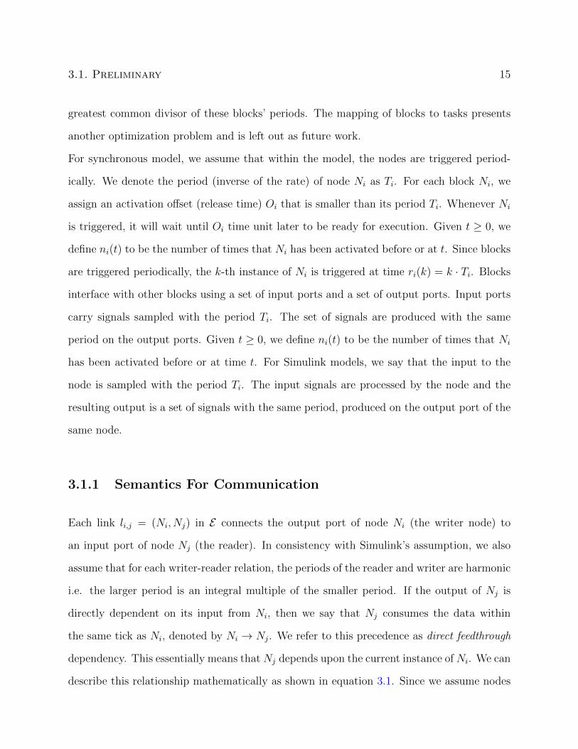
For synchronous model, we assume that within the model, the nodes are triggered period-
ically. We denote the period (inverse of the rate) of node Ni as Ti. For each block Ni, we
assign an activation offset (release time) Oi that is smaller than its period Ti. Whenever Ni
is triggered, it will wait until Oi time unit later to be ready for execution. Given t ≥ 0, we
define ni(t) to be the number of times that Ni has been activated before or at t. Since blocks
are triggered periodically, the k-th instance of Ni is triggered at time ri(k) = k · Ti. Blocks
interface with other blocks using a set of input ports and a set of output ports. Input ports
carry signals sampled with the period Ti. The set of signals are produced with the same
period on the output ports. Given t ≥ 0, we define ni(t) to be the number of times that Ni
has been activated before or at time t. For Simulink models, we say that the input to the
node is sampled with the period Ti. The input signals are processed by the node and the
resulting output is a set of signals with the same period, produced on the output port of the
same node.
3.1.1 Semantics For Communication
Each link li,j = (Ni, Nj) in E connects the output port of node Ni (the writer node) to
an input port of node Nj (the reader). In consistency with Simulink’s assumption, we also
assume that for each writer-reader relation, the periods of the reader and writer are harmonic
i.e. the larger period is an integral multiple of the smaller period. If the output of Nj is
directly dependent on its input from Ni, then we say that Nj consumes the data within
the same tick as Ni, denoted by Ni → Nj. We refer to this precedence as direct feedthrough
dependency. This essentially means that Nj depends upon the current instance of Ni. We can
describe this relationship mathematically as shown in equation 3.1. Since we assume nodes

16 Chapter 3. Mechanisms for Preserving Communication Semantics
are triggered periodically, let Nj(k) denote the k-th instance of Nj. Furthermore, let rj(k)
denote the time this instance is triggered, and ij(k) be its input. The SR semantics specify
that ij(k) equals the output of the last occurrence of Ni, denoted by oi(m). The logical-
time semantics for SR models dictate that the output oi(m) should be triggered before the
k-th occurrence of Nj. Thus the time at which m-th instance of the output update can be
triggered latest is rj(k). By assuming that m-th instance is being triggered at rj(k) we can
define the following equation for direct feedthrough:
ij(k) = oi(m), where m = max {n| ri(n) ≤ rj(k)}. (3.1)
Figure 3.1 illustrates a direct feedthrough relationship between a writer node Ni and a reader
node Nj. The x-axis represents time. In the figure, to ensure direct feedthrough (i.e. to
ensure that the reader reads the most recent value) (a) if TNi< TNj
we have ij(k) = oi(m)
and ij(k + 1) = oi(m + 2), (b) if TNi> TNj
, we have ij(k) = ij(k + 1) = oi(m) and
ij(k + 2) = ij(k + 3) = oi(m+ 1)
The SR semantics also allow for delayed communication, where the delay added is limited
to one unit in Simulink (the more general case of multiple delays are discussed in works such
as [31], [22]). If the communication is delayed, Nj does not depend on the output of the
most recent activation of Ni; instead it now reads the previous value. We denote this by
Ni−1→ Nj. In this case, we say that the k-th instance of reader reads from (m−1)-th instance
of writer (from the previous tick), where m-th instance is the most recent writer instance
that is triggered before k-th instance of reader as shown in equation 3.2
ij(k) = oi(m− 1), where m = max {n|ri(n) ≤ rj(k)} (3.2)
Figure 3.2 shows the effect of adding a unit delay on the communication link. In the

3.1. Preliminary 17
Oi(m) Oi(m+1) Oi(m+2) Oi(m+3)
ij(k) ij(k+1)
rj(k) rj(k+1)
ri(m) ri(m+1) ri(m+2) ri(m+3)
Oi(m) Oi(m+1)
ij(k) ij(k+2)
rj(k) rj(k+2)
ri(m)
rj(k+1)
ri(m+1)
rj(k+3)
Trigger Time
Data Flow
Global Tick
A)
B)ij(k+1) ij(k+3)
Ni
Ni
Nj
Nj
Ni Nj
Figure 3.1: Input/output relation with direct feedthrough on the communication link with(A) TNi
< TNj(B) TNi
> TNj
figure, to ensure unit delay (i.e. to ensure that the reader reads the previous value) (a) if
TNi< TNj
we have ij(k + 1) = oi(m + 1) and similarly ij(k) = oi(m − 1), (b) if TNi> TNj
,
we have ij(k + 2) = ij(k + 3) = oi(m) and similarly ij(k) = ij(k + 1) = oi(m − 1). We
can see that there is more time between the instance at which the output is produced and
the instance at which it is consumed. In this case, the reader does not have to finish its
computation within the same tick thus relaxing the input/output dependency within each
tick of execution. This provides some flexibility in implementing schedulability in the system.

18 Chapter 3. Mechanisms for Preserving Communication Semantics
Oi(m) Oi(m+1) Oi(m+2) Oi(m+3)
ij(k) ij(k+1)
rj(k) rj(k+1)
ri(m) ri(m+1) ri(m+2) ri(m+3)
Oi(m) Oi(m+1)
ij(k) ij(k+2)
rj(k) rj(k+2)
ri(m)
rj(k+1)
ri(m+1)
rj(k+3)
Trigger Time
Data Flow
Global Tick
A)
B)
ij(k+1)ij(k+3)
Ni
Ni
Nj
Nj
Ni Nj
Delay
Figure 3.2: Input/output relation with unit delay on the communication link with (A)TNi
< TNj(B) TNi
> TNj
However, this delay requires additional storage in memory for buffering, as the data remains
in the buffer till the next tick when it is finally consumed by the reader. Furthermore,
the added delay increases end-to-end latency which might cause performance degradation
especially for control algorithms [18], [22]. For safety-critical embedded systems such as
flight management system [20], increasing this end-to-end latency beyond a particular value
will result in an unstable operation. Thus, we need to minimize the unit delay block addition

3.1. Preliminary 19
in a given system to ensure optimal control performance.
In summary, in SR semantics the data exchanged by two communicating blocks must be
clearly defined by the model. With direct feedthrough dependencies, the reader reads the
data produced by the most recent occurrence of the writer. With delayed communication,
data from the previous instance is used. In both cases however, there should be no confusion
and the producer of each data item consumed by a reader is explicitly defined by the model
and the computation of reader and writer should complete before the next tick.
A cyclic dependency is possible if Ni and Nj (directly or indirectly) depend on each other in
a feedthrough dependency. This results in a fixed point problem and can violate determinism
in SR semantics by making the output dependent on scheduling. Simulink simply disallows
such cyclic dependencies. In this work, following the approach in Simulink, we assume that
the system does not have any cyclic dependencies, hence we work only with Directed Acyclic
Graphs in our analysis.
3.1.2 Challenges to Preserving Semantics
When generating software code for Simulink functional models, we must ensure that the
implementation behaves identically to the simulated model. An additional complication
here is that it is relatively easier for the simulation engine to preserve the model semantics
since the engine controls virtual time and blocks are assumed to execute in zero virtual time.
However, in reality blocks take time to execute, and preemptions and scheduling delays may
cause differences between the simulated and implemented signal flows. In addition to the
aforementioned factors, the interference from contention for shared resources may further
add an additional delay to the execution of a block.
While considering these delays, to ensure data integrity, we seek to implement a schedulable

20 Chapter 3. Mechanisms for Preserving Communication Semantics
system that follows the logical-time execution semantics as shown in Figure 3.1 and Figure
3.2. In the following sub-section we discuss how these delays may result in violation of
communication semantics for the generated model.
Impact of Execution Delay on Data Integrity
Ni
Nj
read
write1
trigger time
Nj
read read
Ni
A)
B)
Ni Nj
write2
read
read
write1
Figure 3.3: Impact of Delay on Data Integrity on directfeedthrough with (A) TNi< TNj
(B)TNi
> TNj
Considering the semantics defined in section 3.1.1, we see that the scheduling delays may
violate the data integrity for both cases as following :
. Case 1: The reader depends upon the most recent instance of the writer when triggered,
as shown in Figure 3.3. In this case the implementation should follow the semantics of direct-

3.1. Preliminary 21
feedthrough (as shown in Figure 3.1). We use the dotted blocks to show how the scheduling
delay may result in possible execution windows of the reader. In this figure, we have (A) a
high-rate writer communicating to a low-rate reader and (B) a low-rate writer communicating
to a high-rate reader. For Figure 3.3(A), based upon when the reader starts executing, the
data read by the reader may come from the first instance (write1) or the second instance
of the writer (write2). However, the simulated model semantics from equation (3.1) dictate
that the reader should always read the value provided by the most recent instance of writer
(write1). Similarly, for Figure 3.3(B), the possible execution windows of the first instance of
the reader may result in loss its data integrity.
. Case 2: The reader task reads the previous value of the writer instance when triggered,
Nj
Ni
Nj
Ni
A)
B)
trigger time
Ni Nj
write1 write1
read1 read2
read1
write1 write1 write2
Figure 3.4: Impact of Delay on Data Integrity on a link with unit delay where (A) TNi> TNj
(B) TNi< TNj

22 Chapter 3. Mechanisms for Preserving Communication Semantics
as shown in Figure 3.4. In this case the implementation should follow the semantics of unit
delay (as shown in Figure 3.2). We represent the possible executions of the writer task with
dotted lines. In this figure, we have (A) a low-rate writer communicating to a high-rate
reader (B) a high-rate writer writing to a low-rate reader. Thus for Figure 3.4 (A), we can
see that based upon the release time, the input to the second reader (read2) may be the
same as read1 or an updated value by the writer (write1). However, the simulated model
semantics from equation (3.2) dictate that the input to the reader can only be updated by
the next instance of writer (occurring in the next cycle/tick). Thus within this cycle both the
readers should have same input i.e. read1 and read2 should be same. A functional delay in
this case is clearly needed to allow that the reader gets the input from the previous instance
of the writer, along with an initial input for the first instance of the reader task. Similarly
for Figure 3.4 (B), the reader should execute before the first instance of the writer (write1)
and correspondingly second instance of writer (write2).
We see that for a single-core architecture, Simulink provides a solution to both these problems
as shown below.
3.1.3 Preserving Semantics on Single-core
Simulink solves both of the above mentioned problems as well as ensures data consistency
for single-core using a mechanism known as Rate Transition (RT) blocks [45] (as shown in
Figure 3.5 and Figure 3.6). RT blocks are a special implementation of wait-free methods.
These blocks placed between the writer and the reader (as shown in Figure 3.5 and Figure
3.6), forward appropriate data from the writer to the reader, and provide initial data val-
ues when necessary. RT blocks are only applicable to one-to-one communication. However,
one-to-n communication can still be implemented using RT buffers as n separate one-to-one
links. Furthermore, RT blocks are a restricted version of wait-free methods. Compared to

3.1. Preliminary 23
the generic wait-free methods [13], they require that the sender and receiver have harmonic
periods. Harmonic periods ensure that the larger period is a multiple of the smaller period.
Also, for our analysis we call the larger period to be the hyperperiod. Thus, we need to
ensure that within a given hyperperiod, events happen in the same causality order as the
simulated model.
The RT block comprises of two functions : output update function (denoted by striped box
in our figures) and a state update function (denoted by gridded box in our figures). If we
consider RT block as a buffer, then state update function can be considered as writing the
data into the buffer. Similarly, output update function can be considered as reading the
data from the buffer. Now we see how this RT block can be used to ensure data integrity
for both cases mentioned in previous section.
. Case 1: For the first case mentioned above in Figure 3.3, the RT block needs to behave
like a Zero-Order Hold block as shown in Figure 3.5. Thus RT block buffers the data from
the writer till the next instance of the reader is activated. The RT block’s output update
function (shown by striped box) executes at the rate of the slower block (at the rate of reader
for Figure 3.5 (A) and at the rate of writer for Figure 3.5 (B)) but within the writer block,
thus ensuring that the input to the reader is not updated till the next instance of slower
block is triggered. Also, the state update (shown by gridded box) occurs within the task and
at the priority of the writer block, thus ensuring that the output by each instance of writer
is stored in the buffer. If the writer instance executes before the corresponding reader in the
hyperperiod, we refer to RT blocks associated with this execution order as direct feedthrough
(DF).
. Case 2: For the second case mentioned above in Figure 3.4, the RT block needs to behave
like a Unit Delay block as shown in Figure 3.6. Thus RT block should provide an initial
value in the start and buffer the output from the writer till the next instance of writer is
triggered. The RT block state update function (shown by gridded box) should execute in

24 Chapter 3. Mechanisms for Preserving Communication Semantics
Ni
Nj
hold
read
write
trigger time
Nj
hold
read
write
read
Ni
A)
B)
Ni NjRate Tansi�on
(Hold)
write
Figure 3.5: Preserving Data Integrity by RT blocks for directfeedthrough in single-core with(A) TNi
< TNj(B)TNi
> TNj
the context of the writer task, thus ensuring that the output of each writer instance is stored
in the buffer. The RT block output update function should run in the context of the reader
block, but at the rate of the slower block (at the rate of writer for Figure 3.5 (A) and at
the rate of reader for Figure 3.5 (B)). This will ensure that the reader blocks read the same
value, provided by the previous instance of the writer. For the case when the reader exe-
cutes before the writer when triggered together, we refer to RT blocks associated with this
execution order as Unit Delay (UD). This type of RT blocks results in additional functional
delay equal to the writer’s period as the data produced by the writer will be consumed in
the next period. This causes an adverse effect on the end-to-end latency thus eventually

3.1. Preliminary 25
Nj
Ni
read
hold
readread read
write
Nj
Ni
read
hold
read
write
A)
B)
write
trigger time
Ni NjRate Tansi�on
(Sample-and-Hold)
Figure 3.6: Preserving Data Integrity by RT blocks for unit delay link in single-core with(A) TNi
> TNj(B) TNi
< TNj
degrading the performance of the system [49].
With the above discussion, we see how the Simulink uses RT blocks to preserve the com-
munication semantics on a single-core architecture. The problem becomes more complex for
partitioned multicore architecture as there is no notion of global priority. Hence, in order to
establish an execution order in the multicore architecture we use release time of each task.
In the following section, we first discuss the task model that will be used in our analysis.
Using that task model, we then proceed to explain how this execution order based on release
times can be used to preserve the semantics for multicore architecture.

26 Chapter 3. Mechanisms for Preserving Communication Semantics
3.2 Task Model for Multicore Architecture
We focus here on multitask implementations since they are much more efficient [18] and
allow us to fully utilize a multicore architecture. In multitask implementation of Simulink
models, blocks are mapped to fixed-priority tasks or threads scheduled by an RTOS. In our
work we assume that the core allocation for each task is given to us as an input. We leave
this partitioning scheme as a part of future work.
A task τi implementing node Ni is characterized by the following parameters: Ci, denoting
the task’s Worst Case Execution Time (WCET) free from all interferences; Ti, the task’s
period which is the same as the period of Ni; Di = Ti, the deadline of task i.e. the amount of
time a task has from its trigger time to the time instant at which it must finish its execution;
Ei, the core allocated to the task τi; pi, the task’s priority; αi, the set of tasks that write to
task τi ; βi, the set of tasks that read from τi;
In addition, we use synchronized triggering of tasks, and introduce the offset (release time)
Oi, which is the difference between the trigger time and the activation of the task instance.
For our analysis, we define response time Ri of task τi as the time difference between when
the task finishes execution and the the time it is activated. The communication link between
a writer task τi and reader task τj is denoted as li,j. Furthermore, we denote the presence of
unit delay RT block on a communication link as DBi,j ∀ li,j. We define the response time of
the output update function running in the context of reader τi as RRTi (discussed in section
3.1.3). Further notations are present in Table 5.1 in Chapter 5.
For a schedulable system we calculate the response time for a task and check if the task
finishes before its deadline. We do this by considering both inter core as well as intra core
interference :
• Intra Core Interference : The delay to the execution of task τi rising from all the tasks
3.2. Task Model for Multicore Architecture 27
that preempt the execution of task τi. We denote hp(i) as the set of tasks that belong
on the same core as τi and have a higher priority than τi. Thus for execution window
of Ri, task τi will be preempted at leastRi
Tj∀ j ∈ hp(i). Preemption of τi by τj will
result an addition ofRi
Tj·Cj to the execution of τi. Thus the computed net interference
is given as∑
j∈hp(i)
⌈Ri
Tj
⌉· Cj.
• Inter Core Interference : By using RT blocks and separating the execution windows
of the communicating tasks, we remove the inter-core interference completely from
calculation of response time.
Thus we end up with the calculation of Response Time of the task τi as shown in equation
(3.3)
Ri = Ci +∑
j∈hp(i)
⌈Ri
Tj
⌉· Cj (3.3)
where hp(i) is the set of tasks that have higher priority than τi and are allocated to the same
core. As seen from section 3.1.3 we also need response time of the output update function
to ensure that for the case of unit delay, the writer can execute only after the output update
function is completed. For output update function of RT block RTi running in the context
of the reader task τi, we assume the Worst Case Execution Time (CRT ) to be negligible and
the priority of the output update function to be the same as that of the reader task. By
following the same procedure as calculation of Ri, we compute the response time of output
update function as shown in equation 3.4
RRTi = CRT +∑
j∈hp(i)
⌈RRTi
Tj
⌉· Cj s.t. CRT ≈ 0 (3.4)
Thus essentially the output update function has a response time equal to the net interference

28 Chapter 3. Mechanisms for Preserving Communication Semantics
occurring due to preemption of task τi by other tasks running on the same core. Now that
we have defined the task model and the semantics of communication, we move towards
discussing how the communication semantics for this task model are preserved.
3.3 Preserving Semantics on Multicore Architecture
In partitioned multicore architectures, we need to ensure that the generated execution order
follows the simulated causality order while preserving the communication semantics as done
for single-core in Figure 3.5 and Figure 3.6. To do so, we need to make sure that the partial
execution order between any two communicating blocks Ni and Nj follows the semantics
between the writer and reader as shown in Figure 3.1 and Figure 3.2.
Definition 3.1. We define a partial execution order fi,j in our system to denote that
block Ni executes before block Nj whenever they are triggered together.
Example 3.2. In Figure 3.5, we say that the partial execution order between Ni and Nj is
fi,j, as Ni executes before Nj in the hyperperiod. similarly, for Figure 3.6, we say that the
partial execution order between Ni and Nj is fj,i.
In this section, we use definition 3.1 to formally define how the partial execution order
should be used to preserve the communication semantics for both inter-core and intra-core
communication links.
3.3.1 Preserving Intra-core Communication Semantics
When the reader and writer are assigned to the same core, we have a well-defined priority
order to determine the execution order of the generated model. Thus the execution order in
3.3. Preserving Semantics on Multicore Architecture 29
this case should follow the semantics as defined for single-core in Figure 3.5 and Figure 3.6.
. Case 1: The reader instance is directly dependent upon the output from the current
writer instance. Thus the execution of the writer block Ni is followed by the execution of
the corresponding reader instance Nj, as shown in Figure 3.7. This partial execution order
should ensure that the system follows the the semantics of Figure 3.1. For this case, the RT
block should behave like a directfeedthrough RT block. Thus the state update function is
executed within the writer task and the output update function (striped box) is executed at
the rate of the slower block. To ensure that partial execution order fi,j follows the semantics
of equation (3.1), we (a) assign block Ni higher priority than block Nj and (b) activate Ni
before Nj. If we assume the activation time of block Ni is Oi and the priority is pi, we say
that:
Principle 1. For a given intra-core communication link from Ni to Nj, execution order fi,j
enforces the following constraint to imply the use of a directfeedthrough RT block :
Oi ≤ Oj
∧pi > pj (3.5)
. Case 2: The reader instance depends upon the previous instance of the writer. Thus,
reader Nj executes before writer block Ni when triggered together, as shown in Figure 3.8.
The semantics for this execution order should follow the semantics for a relaxed dependency
as shown in Figure 3.2. For this case, the RT block behaves like a Unit Delay block plus
a Hold block (Sample and Hold). Thus the state update function (gridded box) executes
within the writer block and the output update function (striped box) executes in context
of reader at the rate of the slower block. To ensure that partial execution order fj,i follows
the semantics of equation (3.2) we (a) assign block Nj higher priority than block Ni and (b)

30 Chapter 3. Mechanisms for Preserving Communication Semantics
Ni
Nj
Oi
Oj Oi
hold
read
write
trigger
time
activation
time
Nj
Oj Oi
hold
read
write
Oi
read
Ni
A)
B)
Figure 3.7: Preserving the communication semantics for Intra-core directfeedthrough Linkwith (A) TNi
< TNj(B) TNi
> TNj
activate the output update function before Ni. If we assume the activation time of block Ni
is Oi and the priority is pi, we say that
Principle 2. For an intra-core communication link from Ni to Nj, fj,i implies the use of a
unit delay RT block and enforces the following constraint:
Oj ≤ Oi
∧pi < pj (3.6)
Now, we proceed to see how this semantics-preserving execution order can be defined for
inter-core communication links.

3.3. Preserving Semantics on Multicore Architecture 31
Nj
Ni
Oj
Oi Oj
read
hold
readread read
write
Nj
Ni
Oj
Oi Oj
read
hold
read
write
A)
B)
write
Figure 3.8: Preserving the communication semantics for Intra-core unit-delay Link with (A)TNi
> TNj(B) TNi
< TNj
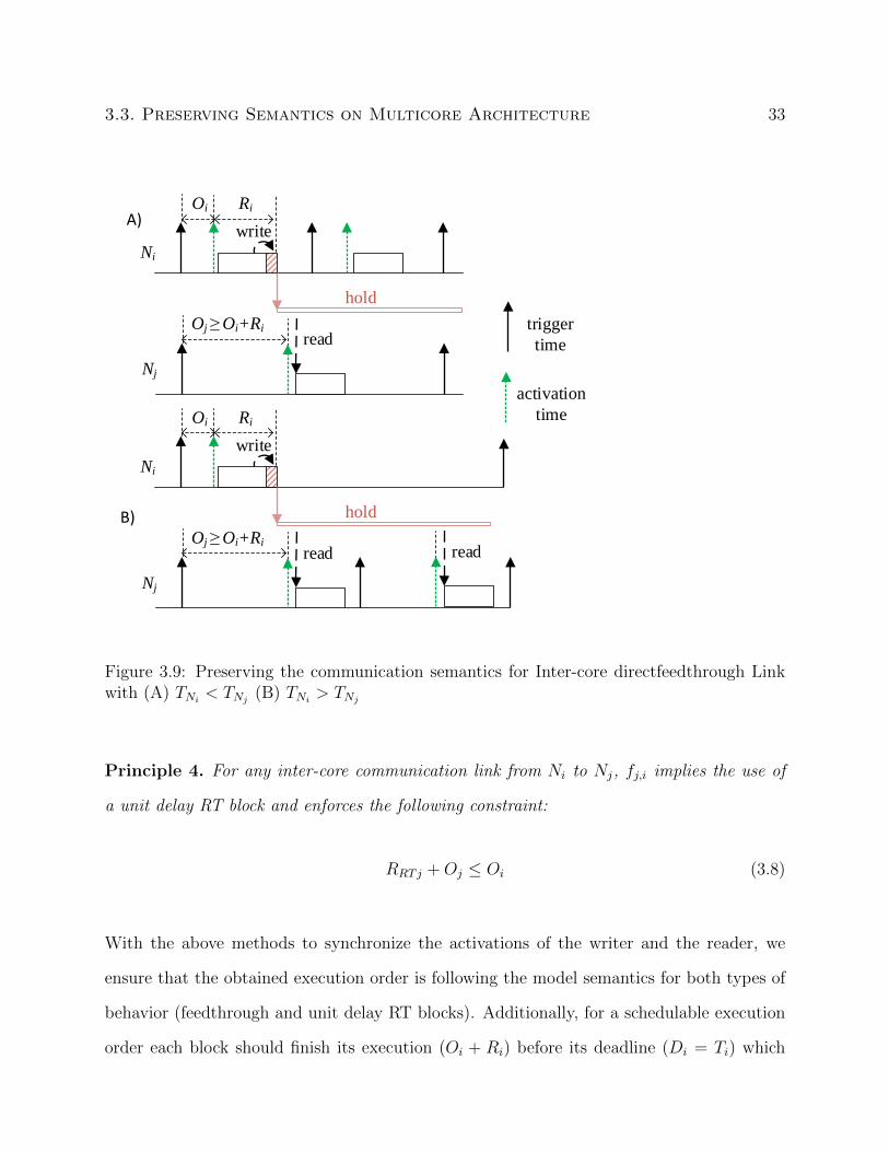
3.3.2 Inter-core Communication Semantics
When the reader and writer blocks are assigned to different cores with partitioned scheduling,
preserving the SR semantics is more challenging since there is no notion of global priority.
We consider a mechanism that combines the RT block and offset assignment, the later assign
a release offset to blocks to separate the execution windows of the communicating blocks on
different cores and enforce a global execution order. The behavior of RT block in multicore
is the same as that for the single-core as shown in Figure 3.5 and Figure 3.6.
. Case 1: The reader instance directly depends upon the current writer instance. Thus, the
writer block Ni executes before the corresponding reader Nj, and we use a directfeedthrough

32 Chapter 3. Mechanisms for Preserving Communication Semantics
RT block as shown in Figure 3.9. This execution order follows the semantics of Figure 3.1
such that the output update function (striped box) runs within the writer block at the rate
of the slower block. For inter-core link, the partial order fi,j can preserve the semantics
of equation (3.1) by activating the reader Nj with an offset Oj that should be no smaller
than the sum of the worst case response time Ri and the offset Oi of the writer block Ni.
This ensures that the state update function is executed and the buffer holds the latest value
before the reader is activated. If we assume the activation time of block Ni is Oi and the
response time is Ri, we say that:
Principle 3. For any inter-core communication link from Ni to Nj, fi,j implies the use of
a directfeedthrough RT block and enforces the following constraint:
Ri +Oi ≤ Oj (3.7)
. Case 2: The input to the reader depends upon the previous instance of the writer. This
execution order should follow the semantics of Figure 3.2. Thus, the writer block Ni starts
executing after the output update function (striped box) is executed, as shown in Figure 3.10.
Hence we need to ensure that the state update function (gridded box) cannot update the
RT block before the reader has the chance to read it, as shown in Figure 3.6. We can ensure
fj,i preserves the semantics of equation (3.2) by activating the writer Ni with an offset Oi
no smaller than the offset Oj of the reader Nj plus the worst case response time RRTj of the
output update function of the RT block (executing in the context of Nj). If we assume the
activation time of block Nj is Oj and the response time of the output update function (in
the context of reader Nj) is RRTj, we say that
3.3. Preserving Semantics on Multicore Architecture 33
Ni
Nj
Oi
Oj Oi+Ri
hold
read
write
trigger
time
activation
time
Ri
Ni
Nj
Oi
Oj Oi+Ri
hold
read
write
Ri
read
A)
B)
Figure 3.9: Preserving the communication semantics for Inter-core directfeedthrough Linkwith (A) TNi
< TNj(B) TNi
> TNj
Principle 4. For any inter-core communication link from Ni to Nj, fj,i implies the use of
a unit delay RT block and enforces the following constraint:
RRTj +Oj ≤ Oi (3.8)
With the above methods to synchronize the activations of the writer and the reader, we
ensure that the obtained execution order is following the model semantics for both types of
behavior (feedthrough and unit delay RT blocks). Additionally, for a schedulable execution
order each block should finish its execution (Oi + Ri) before its deadline (Di = Ti) which

34 Chapter 3. Mechanisms for Preserving Communication Semantics
Nj
Ni
Oj
read
hold
readread read
write
Oi ≥ Oj+𝑅𝑅𝑇𝑗
𝑅𝑅𝑇𝑗
Nj
Ni
Oj
read
hold
read
write
Oi ≥ Oj+𝑅𝑅𝑇𝑗
𝑅𝑅𝑇𝑗
A)
B)
Figure 3.10: Preserving the communication semantics for Inter-core Link with Unit-Delaywith (A) TNi
> TNj(B) TNi
< TNj
adds another constraint for each block.
Ri +Oi ≤ Ti , ∀i (3.9)
Thus for a reliable software synthesis, we see that the generated execution order should
preserve the communication semantics for multicore architecture for both feedthrough and
unit delay RT blocks while ensuring schedulability. Furthermore, we need to reduce the
number of unit delay RT blocks in the system for optimal performance. In the following
chapter, we proceed to formulate the problem to see how the generated implementation can
provide optimal performance while preserving the semantics for simulated model.

Chapter 4
Problem Formulation
Now that the semantics for communication have been defined, we can now focus on formally
defining the optimization problem for a given system (introduced in Chapter 1). In this work,
we are interested in providing a generated implementation that follows the semantics of the
simulated model and adds minimal unit delay in the system. As seen from equations (3.5),
(3.6), (3.7) and (3.8) computing this execution order further involves: assigning priorities to
tasks, assigning offsets to all tasks, and assigning delays to communication links. The design
constraint is to ensure schedulability on all cores by meeting the deadlines of all tasks (as
shown in equation (3.9)). The objective is to minimize the unit delay block count added by
the execution order while ensuring schedulability.
For a link τi → τj, we use the principles 1, 2, 3, 4 (defined in section 3.3) to say that
• partial execution order fi,j implies the use of direct-feedthrough RT block i.e. DBi,j =
0. Additionally, to ensure that the generated model follows the logical-time execution
semantics, design constraints (3.5), (3.7) and (3.9) should be satisfied
• partial execution order fj,i implies the use of a unit-delay RT block i.e. DBi,j = 1.
Additionally, to ensure that the generated model follows the logical-time execution
semantics, design constraints (3.6), (3.8) and (3.9) should be satisfied
Thus our optimal software synthesis should find an execution order that follows the commu-
nication semantics of the simulated model and adds minimal functional delay in the system.
35

36 Chapter 4. Problem Formulation
To represent this problem in a mathematical form, we introduce a helper binary variable ti,j
defined as
ti,j =
1, fi,j is enforced
0, otherwise
(4.1)
Each link li,j introduces two binary variables ti,j and tj,i corresponding to two possible partial
execution orders. The optimization problem can then be formally expressed as
min∀P,O,t
∑∀li,j
wi,j · tj,i
s.t. P,O satisfy the implied design contraint by fi,j, ∀li,j
Ri +Oi ≤ Di, ∀i
ti,j + tj,i = 1, ∀i 6= j
ti,j ≥ ti,k + tk,j − 1, ∀i 6= j 6= k
(4.2)
where P = [p1, ...pn] and O = [O1, ...On] represent the vectors of priority and offset assign-
ment respectively, t = [ti,j, tj,i|li,j] is the set of execution order variables, and wi,j is the cost
on adding a functional delay to the link li,j. Thus formulation (4.2) seeks to find the minimal
cost of unit delay addition for all possible priority orders, offset assignment and execution
orders while ensuring the schedulability of the system. The last two sets of constraints cor-
respond to anti-symmetry and transitivity of the partial execution orders and are used to
ensure that a valid execution order exists. The former means that if τi has a higher order
than τj (ti,j = 1), then τj must have a lower order than τi (tj,i = 0). The later enforces that
if τi has a higher order than τk (ti,k = 1) and τk has a higher order than τj (tk,j = 1), then τi
must have a higher order than τj (ti,j = 1).In the following chapter, we discuss the proposed
solutions that we use to solve the optimal software synthesis problem for the defined system
model.

Chapter 5
MILP Formulation
In this chapter, we discuss the standard MILP formulation that solve the optimization prob-
lem described in Section 4. We discuss a Mixed Integer Linear Programming (MILP) for-
mulation that essentially converts the model into a set of mathematical equations and then
solves those equations in accordance with a defined objective. To find the optimal solution,
MILP uses branch and cut algorithm and applies cuts at every node to remove infeasible
solutions till it finally reaches an optimal solution. However, this method of analysis makes
it unscalable, as for larger systems the model becomes too huge and the branch and cut
algorithm takes too much time to find the optimal solution. To get the solution quickly for
large systems we then introduce a more efficient framework which finds the same optimal
solution as MILP but has a much less run-time as compared to MILP (shown in Chapter 6).
Within this MILP formulation, we will use notations present in Table 5.1. As mentioned in
Section 4, the problem for finding the optimal execution order involves
• assigning priorities to tasks such that constraints (3.5), (3.6) are satisfied
• assigning offset and response time assignment such that constraints (3.5), (3.6), (3.7),
(3.8) and (3.9) are satisfied
• ensuring minimal unit delay RT block count
After defining all the constraints and the objective function in terms of mathemati-
cal equations, we use IBM ILOG CPLEX Optimization studio [1] to solve the model.
37

38 Chapter 5. MILP Formulation
Symbol Meaning
Γ = Task Set containing all tasks
Pi,j = Priority of task τi with respect to τj
Ri = Response Time of Task τi
RRTi = Response Time of output update function of reader task τi
li,j = Link between writer τi and reader τj
fi,j = Partial execution order between τi and τj
F = Execution order set
αi = Set of tasks writing to task τi
βi = Set of tasks reading from task τi
Ei = Core allocated to Task τi
Di = Deadline of task τi
Ti = Time Period of task τi
Ci = Worst case Execution Time of task τi
hp(i) = Set of tasks having higher priority than τi
lp(i) = Set of tasks having lower priority than τi
pi = priority assigned to task τi
RiLB= Lower Bound of Ri
RiUB= Upper Bound of Ri
RRTiLB= Lower Bound of RRT i
RRTiUB= Upper Bound of RRT i
Θ = Set of Offset constraints Oi∀i
Ij,i = Number of times τj ∈ hp(i) preempts τi
Lj,i = Number of times τj preempts τi
Table 5.1: Notations Used in our implementation

39
Constraint 1 - Valid Priority Order
A binary decision variable Pi,j is set to 1, if and only if priority of task τi is greater than
that of task τj while task τi and τj are on the same core i.e. τi ∈ hp(j). If Pi,j = 1 then
accordingly Pj,i must be zero. This logical constraint can be given as:
∀τi 6= τj ∧ Ei = Ej : Pi,j + Pj,i = 1 (5.1)
From the definition of transitivity, if task τi has higher priority than task τj (i.e. Pi,j = 1),
and task τj has higher priority than task τk (i.e. Pj,k = 1), then task τi has higher priority
than τk , i.e. Pi,k = 1. This logical constraint can be linearized as:
∀τi 6= τj 6= τk ∧ Ei = Ej = Ek : Pi,j + Pj,k ≤ 1 + Pi,k (5.2)
We add constraints (5.1) and (5.2) to ensure that the MILP finds a fixed solution to the
priority assignment of the system Γ where every task τi has a unique priority pi. Now we
move towards response time analysis to ensure that constraint (3.9) is satisfied.
Constraint 2 - Response Time Computation
During its execution task τi will be preempted by high priority tasks running on the same
core. A integer decision variable Ij,i is used to represent the number of times task τi will be
preempted by task τj ∈ hp(i) during its execution time Ri. The constraint can be shown as:
∀τi 6= τj ∧ Ei = Ej : Ij,i ≥Ri
Tj(5.3)
By including the priority order (Pj,i) as a design variable, we define a positive integer Lj,i as
the number of times a task τj preempts task τi on the same core. The given constraint can

40 Chapter 5. MILP Formulation
be linearized by using big M notation as shown below :
∀τi 6= τj ∧ Ei = Ej : Lj,i ≥ Ij,i − (1− Pj,i)⌈Di
Tj
⌉(5.4)
Remark 5.1. For the case of Pj,i = 1 the constraint (5.4) reduces to constraint (5.3), whereas
for Pj,i = 0, it reduces to Lj,i ≥Ri
Tj−
⌈Di
Tj
⌉. Since Ri ≤ Di and Lj,i is a positive integer,
for Pj,i = 0 we get Lj,i ≥ 0. Thus we see that Pj,i = 0 adds no additional constraint, hence
ensuring that the low priority tasks do not affect the execution time of τi.
After the calculation of interference from preemption we calculate the response time as done
in Section 3.2. As denoted by equation (5.4) the decision variable Lj,i represents the times
task τj interferes with task τi. Thus the net response time for task τi considering intra core
interferences, can be linearized as:
∀τi 6= ∀τj ∧ Ei = Ej : Ri = Ci +∑j
Lj,i · Cj (5.5)
For computing the response time of the output update function RRTi, we follow the similar
procedure above. We assume the WCET of RT output update function to be nearly 0
(10−5 for our analysis) and priority equal to that of task τi. Thus, we obtain the following
constraint for calculating RRTi:
∀τi 6= ∀τj∧ : Ei = Ej :
Ij,i ≥RRTi
Tj∧ Lj,i ≥ Ij,i − (1− Pj,i)
⌈Di
Tj
⌉∧ RRTi = CRTi +
∑j
Lj,i · Cj
(5.6)
Additionally, we need to ensure that the output update function finishes its execution before
41
the reader task τi. Thus, we add the following constraint:
∀τi : RRTi ≤ Ri − Ci (5.7)
Constraint 3 - Ensuring System Schedulability
The system can be made schedulable by adding the following constraint:
∀τi : Ri +Oi ≤ Di (5.8)
Constraint 4 - Execution order
For any two communicating tasks τi and τj, we need to have a unique defined partial execution
order, thus we add the following anti-symmetric constraint to denote the presence of a single
execution order
∀ti,j : ti,j + tj,i = 1 (5.9)
For tasks communicating on the same core, since ti,j = 1 implies priority order Pi,j = 1, thus
we can add transitivity constraint (5.2):
∀τi 6= τj 6= τk on the same core: ti,j + tj,k ≤ 1 + ti,k (5.10)
The design constraints imposed by the partial execution order are as following:
IFor Intra-core communication link
By principles 1 and 2, partial execution order fi,j ≡ (ti,j = 1) avoids the use of a delay block
and enforces constraint (3.5). Otherwise for the partial execution order fj,i ≡ (tj,i = 1), we
add a unit delay block and constraint (3.6). This can be formulated with the following linear

42 Chapter 5. MILP Formulation
constraints
∀li,j : Ei = Ej :
Oj ≤ Oi + ti,j ·Dj ∧ Oi ≤ Oj + tj,i ·Di ∧ DBi,j = tj,i
(5.11)
Thus, we can see that for ti,j = 1 constraint (3.6) i.e. Oj ≤ Oi + Dj becomes a trivial
constraint that is already included in constraint (5.8). Similarly, for tj,i = 1 constraint (3.5)
i.e. Oi ≤ Oj +Di becomes a trivial constraint.
I Inter-Core communication Link :
By principles 3 and 4, partial execution order fi,j ≡ (ti,j = 1) avoids using a delay block and
enforces constraint (3.7). Otherwise for the partial execution order fj,i ≡ (tj,i = 1), we add
a unit delay block and constraint (3.8). This can be formulated with the following linear
constraints:
∀li,j : Ei 6= Ej :
Oi +Ri ≤ Oj + tj,i ·Di ∧Oj +RRTj ≤ Oi + ti,j ·Dj ∧DBi,j = tj,i
(5.12)
Following the similar logic as shown for intra-core links, ti,j = 1 makes design constraint
(3.8) for unit delay block trivial and tj,i = 1 makes the constraint (3.7) for direct-feedthrough
trivial.
Objective:
The objective function of this MILP model is to minimize the weighted sum of number
of delay blocks added by the execution order while ensuring all the above constraints are
satisfied.
min∀li,j
∑wi,j · tj,i (5.13)
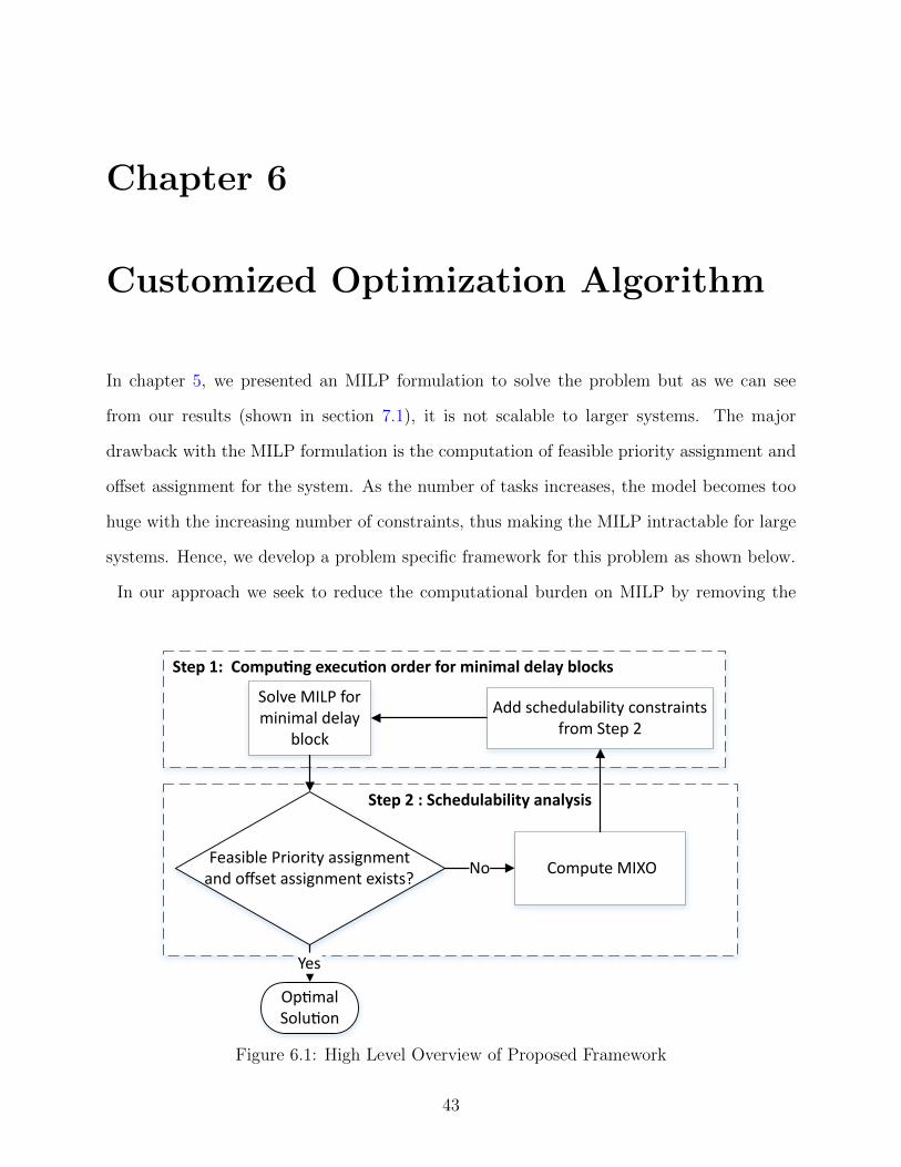
Chapter 6
Customized Optimization Algorithm
In chapter 5, we presented an MILP formulation to solve the problem but as we can see
from our results (shown in section 7.1), it is not scalable to larger systems. The major
drawback with the MILP formulation is the computation of feasible priority assignment and
offset assignment for the system. As the number of tasks increases, the model becomes too
huge with the increasing number of constraints, thus making the MILP intractable for large
systems. Hence, we develop a problem specific framework for this problem as shown below.
In our approach we seek to reduce the computational burden on MILP by removing the
Step 2 : Schedulability analysis
Step 1: Compu�ng execu�on order for minimal delay blocks
Solve MILP for minimal delay
block
Feasible Priority assignment and offset assignment exists?
Yes
No Compute MIXO
Op�mal Solu�on
Add schedulability constraints from Step 2
Figure 6.1: High Level Overview of Proposed Framework
43

44 Chapter 6. Customized Optimization Algorithm
computation of response time assignment, offset assignment and priority assignment from the
MILP. This computation is handled by a dedicated algorithm, which is more efficient than
formulating a standard MILP. By doing so, we effectively divide the problem of obtaining
the optimal execution order (as shown in equation (4.2)) into a two step iterative problem as
shown in Figure 6.1. In step 1 we use a simplified MILP model that focuses on the objective
and tries to impose directfeedthrough on as many links as possible, without considering
any constraints for offset assignment or priority assignment. In step 2 we confirm that a
feasible priority assignment and offset assignment exists that satisfies the design constraints
enforced by the execution order obtained from step 1 (thus focusing on the schedulability part
of equation (4.2)). Otherwise, we define the concept of Minimal Infeasible eXecution
Order (MIXO) as an abstraction of the partial execution order that makes the system
unschedulable. We use the results from step 2 to gradually shape the feasibility region of
the MILP till we obtain an execution order which is schedulable. Thus essentially, we start
with enforcing directfeedthrough on all links and during the runtime, we effectively learn
which links require the addition of delay block for schedulability. The concept of using the
schedulability constraints to shape feasibility of MILP is similar to that of the unschedulable
core guided optimization presented by Zhao and Zeng [52]. In this section, we formally define
MIXO and how we use it for our framework.
Definition 6.1. For a given system, we define execution order set F = {fi1,j1 , .., fim,jm}
as the set of the partial execution orders that exist across the communication links of the
system. The number of elements in F can be defined as its cardinality, denoted by |F |.
Definition 6.2. To confirm that the system is schedulable for a given execution order F ,
we say that the task system Γ is said to be F -feasible if there exists
• a feasible priority assignment that satisfies the partial priority order Pi,j = 1 for each
element fi,j in F by Principles 1 and 2 (as shown in equations (3.5) and (3.6))

45
• a feasible offset assignment that satisfies the offset constraints added by each element
fi,j in F by Principles 1, 2, 3 and 4 (as shown in equations (3.5), (3.6), (3.7) and (3.8))
along with the following constraint
∀i : Ri +Oi ≤ Di (6.1)
If the system is F -feasible, then we say that a feasible priority assignment and offset as-
signment exists that can satisfy all the design constraints imposed by F , thus ensuring
schedulability. In this work, we use the terms like ”feasible execution order”, ”F -feasibility”
etc. to show that the system is F -feasible. Likewise, we say that the system ”does not have
feasible F”, ”F -infeasibility” if the system is not F -feasible. The following example can
elaborate on how we can determine if the system is F -feasible.
τi Ti Di Ci Ei
0 100 100 20 01 100 100 40 02 20 20 10 13 200 200 96 1
Core 0
Core 1
0
3
1
2
Table 6.1: Example Test Case
Example 6.3. Considering the Task System shown in Table 6.1, for execution order set
F = {f0,1, f2,1, f3,2, f3,0}. The system Γ is said to be F -feasible if it has a feasible priority
assignment and an offset assignment that satisfies the constraints (3.5),(3.6),(3.7) and (3.8)
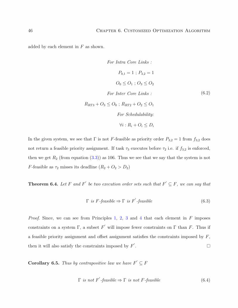
46 Chapter 6. Customized Optimization Algorithm
added by each element in F as shown.
For Intra Core Links :
P0,1 = 1 ; P3,2 = 1
O0 ≤ O1 ; O3 ≤ O2
For Inter Core Links :
RRT3 +O3 ≤ O0 ; RRT2 +O2 ≤ O1
For Schedulability:
∀i : Ri +Oi ≤ Di
(6.2)
In the given system, we see that Γ is not F -feasible as priority order P3,2 = 1 from f3,2 does
not return a feasible priority assignment. If task τ3 executes before τ2 i.e. if f3,2 is enforced,
then we get R2 (from equation (3.3)) as 106. Thus we see that we say that the system is not
F -feasible as τ2 misses its deadline (R2 +O2 > D2)
Theorem 6.4. Let F and F′
be two execution order sets such that F′ ⊆ F , we can say that
Γ is F -feasible⇒ Γ is F′-feasible (6.3)
Proof. Since, we can see from Principles 1, 2, 3 and 4 that each element in F imposes
constraints on a system Γ, a subset F′
will impose fewer constraints on Γ than F . Thus if
a feasible priority assignment and offset assignment satisfies the constraints imposed by F ,
then it will also satisfy the constraints imposed by F′.
Corollary 6.5. Thus by contrapositive law we have F′ ⊆ F
Γ is not F′-feasible⇒ Γ is not F -feasible (6.4)
6.1. Problem Formulation for MIXO Framework 47
This essentially means that if the constraints imposed by F′
make the system unschedula-
ble, then the system will definitely be unschedulable for any superset of F′. Now that we
know how to confirm the schedulability of the system for a given execution order, we can
reformulate the optimization problem as below.
6.1 Problem Formulation for MIXO Framework
From definition 6.2, we can say that if the system is F -feasible, then a feasible priority
assignment and offset assignment exists. From section 4, we see that for link li,j, partial
execution order fj,i ≡ (tj,i = 1) denotes the presence of unit delay block and fi,j ≡ (ti,j = 1)
denotes the absence of the delay block. In order to obtain the optimal execution order shown
in equation (4.2), we formulate the problem as:
min∀F
∑∀li,j
wi,j · tj,i
s.t. Γ is F -feasible
ti,j + tj,i = 1, ∀i 6= j
ti,j ≥ ti,k + tk,j − 1, ∀i 6= j 6= k
(6.5)
By reformulating the problem as above, we can split the problem into two parts such that
MILP deals with the minimization of the objective and the feasibility analysis checks if the
system is F -feasible (as mentioned in definition 6.2). From the perspective of the reformu-
lated problem (6.5), Corollary 6.5 suggests that if a partial execution order set F ′ is known
to be infeasible, then the search for the optimal feasible F shall avoid any superset of F ′.
Thus an infeasible partial execution order set F ′ provides a clue for performing search space
reduction for the MILP. Intuitively, the smaller the F ′, the greater the number of infeasible
partial execution order sets it can capture. To do so, we use the concept of MIXO as an

48 Chapter 6. Customized Optimization Algorithm
irreducible abstraction of the execution order set that makes the system unschedulable. We
define the concept of MIXO as shown below.
Definition 6.6. By using corollary 6.5 and definitions 6.1, 6.2, we define an execution order
set U as a minimal infeasible execution order set (MIXO) if and only if
• Γ is not U -feasible
• ∀F ′ ⊂ U , Γ is F′-feasible
Remark 6.7. By theorem 6.4, the second condition can be formulated as
∀F ′ ⊂ U s.t. |F ′| = |U | − 1, Γ is F′-feasible (6.6)
Example 6.8. For system in Table 6.1, we see that for F = {f3,2, f0,1}, Γ is not F -feasible
as P3,2 = 1 is not a feasible priority order. However F is not a MIXO as Γ is still infeasible
for F′
= {f3,2}, where F′ ⊂ F . But we see that F
′is a MIXO as Γ is not F
′-feasible but is
F′′-feasible where F
′′= {φ} is a subset of F
′.
For the computed MIXO U , by definition 6.6 all the enforced partial execution orders in
U cannot be simultaneously satisfied. Thus by using equation (6.6) we use the following
constraint to obtain a subset of the enforced execution order set F′
s.t. the system is F′-
feasible : ∑∀fi,j∈U
ti,j ≤ |U | − 1 (6.7)
By using the equation (6.7), we can add the feasibility constraints for each obtained MIXO
to shape the feasibility region of the MILP. We see that for a given execution order set, we
can obtain the MIXO as explained below.

6.2. MIXO Computation 49
6.2 MIXO Computation
For a given execution order set and a system Γ, we use algorithm 1 to compute the minimal
infeasible execution order set F . In algorithm 1, we remove each partial execution order one
by one to check if Γ becomes F -feasible. If removing fi,j makes Γ F -feasible, we keep fi,j
in F as it is an infeasible execution order that makes the system unschedulable. However,
if removing fi,j does not change the schedulability of the system, then we can say that it is
not a cause of unschedulability. By iterating through all elements of F , the function returns
a computed set of minimal infeasible execution order F such that Γ is not F -feasible but Γ
is F′-feasible ∀F ′ ⊂ F .
The following example shows how we can use Algorithm 1 to compute the MIXO for a given
execution order set F .
input : Execution order set F , Task Set Γoutput: Minimal Infeasible Execution Order set F
1 forall fi,j ∈ F do2 Remove fi,j from F ;3 if Γ is F-feasible then4 Keep fi,j in F ;5 end6 else7 Remove fi,j from F ;8 end
9 end10 return F ;
Algorithm 1: MIXO Computer
Example 6.9. Continuing from example 6.3, we see that Γ is not F -feasible. By using
algorithm 1, we start with F = {f0,1, f2,1, f3,2, f3,0} and iteratively remove fi,j till we see
that removing fi,j makes the system F -feasible.
We see that removing f3,2 makes the system F -feasible s.t. F = {f3,0}. Thus we put back
f3,2 in F and continue to remove f3,0.

50 Chapter 6. Customized Optimization Algorithm
We see that removing f3,0 does not make the system schedulable and hence remove f3,0 from
F . Thus, we get f3,2 is obtained as the sole reason for unschedulability. We thus obtain the
MIXO as F = {f3,2}. Following equation 6.7, the resultant schedulability constraint added
to the MILP is t3,2 ≤ 0.
From the algorithm 1, we can see that the primary step in computing MIXO is checking
if the system is F -feasible. Thus for a given F , to compute a single MIXO we check the
feasibility |F | times. In the following section, we discuss how we can optimize this analysis
to ensure faster computation of MIXO.
6.3 Feasibility Analysis for MIXO Based Framework
To check if the given system Γ is F -feasible, we need to check if a feasible priority assignment
and offset assignment exists as shown in definition 6.2. To do so, we need to formulate a
mathematical formulation to ensure that all the constraints enforced by the execution order
F are satisfied. Thus for every element in F , we add the design constraints (3.5), (3.6) (3.7),
(3.8) and (3.9) to confirm if a feasible priority assignment and offset assignment exists. For
a given F , the offset assignment should satisfy the following constraints:
∀i : Ri +Oi ≤ Di
For Intra core links from τi to τj:
∀fi,j : Oi ≤ Oj
∀fj,i : Oj ≤ Oi
For Inter core links from τi to τj:
∀fi,j : Ri +Oi ≤ Oj
∀fj,i : RRTj +Oj ≤ Oi
(6.8)

6.3. Feasibility Analysis for MIXO Based Framework 51
At the same time, the feasible priority assignment should satisfy the following constraint
For Intra core links from τi to τj:
∀fi,j : Pi,j = 1
∀fj,i : Pj,i = 1
(6.9)
6.3.1 Exact Feasibility Analysis
We call this feasibility analysis exact as it can find all the schedulability constraints required
to obtain a feasible execution order set. For a system to be F -feasible, it needs a feasible
offset assignment that satisfies the constraints shown in (6.8) as well as a feasible priority
assignment that satisfies (6.9). Since solving this mathematical formulation can be quite
complex, we use the concept of Maximal Unschedulable Deadline Assignment (MUDA) [51]
to determine if a feasible priority assignment and offset assignment exists. MUDA based
framework reformulates the problem into finding a schedulable virtual deadline assignment
that satisfies the constraints in equation (6.8) and (6.9). Virtual deadline di used in this
framework is essentially the maximum feasible upper bound on the response time of a task
and is defined as:
∀ τi : Ri ≤ di s.t. Ci ≤ Ri ≤ Di (6.10)
This framework essentially divides the problem into two components such that the MILP
only solves for the constraints in (6.8) and the responsibility of assigning priorities satisfying
(6.9) is left to another sub-function. The working of MUDA-framework is as following
1. A MILP is used to solve the constraints enforced for offset assignment shown in equation
(6.8), denoted by G(X) ≤ 0. This MILP returns a feasible virtual deadline assignment
without worrying about priority assignment. However, if no such feasible deadline
assignment exists then we return that the system is not F -feasible.

52 Chapter 6. Customized Optimization Algorithm
Solve MILP G(x) ≤ 0
Feasible Priority exists? NoCompute Deadline constraints using
MUDA
Schedulable Deadline Assignment
Yes
Feasible Deadline Assignment
Yes
Feasible Solu�on? Return UnschedulableNo
Figure 6.2: MUDA Framework Overview
2. We confirm if the system has a feasible priority assignment for the feasible deadline
assignment obtained from MILP. Otherwise, we calculate MUDA as an abstraction of
the virtual deadline assignment that makes the system unschedulable. This MUDA is
then added as a deadline constraint to refine the MILP search space till a schedulable
deadline assignment is obtained.
If the MUDA framework (as shown in Figure 6.2) can return a schedulable deadline
assignment, we say that the system is F -feasible. To determine schedulability, we check if
a feasible priority assignment exists, using revised version of Audsley’s algorithm [4]. In
our revised algorithm, we iteratively pick a task and try to assign it a priority p, starting
with the lowest priority first. While choosing the candidate, we need to ensure that (a) the
response time of task at priority level p (as calculated by equation (3.3)) is not greater than

6.3. Feasibility Analysis for MIXO Based Framework 53
the virtual deadline computed by MILP and (b) the net priority assignment follows the
partial order enforced by the execution order (as shown in equation (6.9)). For example, for
fi,j ∈ F , for intra-core links we need to ensure that we assign priority to task τi only if task
τj has already been assigned a lower priority.
Example 6.10. For system shown in Table 6.1, with F = {f0,1, f3,0.f2,3, f2,1}, we use MUDA-
framework to check if the system is F -feasible. The MUDA framework reformulates the
problem into two parts:
Deadline constraints: Partial priority order (PPO) constraints:
O1 ≥ O0 p0 > p1
O2 ≥ O3 p3 > p2
O2 ≥ d1 +O1
O3 ≥ d0 +O0
di +Oi ≤ Ti, ∀τi
Di ≥ di ≥ Ci ∧ di ≥ Ri, ∀τi
(6.11)
For the first iteration, the MILP solves the deadline constraints and provides the feasible
virtual deadline assignment
[d0, d1, d2, d3, dRT2, dRT3] = [20, 40, 10, 96, 0, 10] (6.12)
Now, we use the revised Audsley’s algorithm to check if a feasible priority assignment exists
for deadline assignment (6.12). This priority assignment has to also satisfy the priority
constraints in (6.11). Using our revised Audsley’s algorithm, we determine that for feasible
priority assignment, τ3 cannot have a virtual deadline less than 196. Thus, we obtain MUDA

54 Chapter 6. Customized Optimization Algorithm
as an abstraction of this unschedulable deadline and add it to the MILP as a constraint, to
shape its feasibility region.
d3 ≥ 196 (6.13)
In the next iteration the MILP considers constraint (6.13) and provides the virtual deadline
assignment and the offset assignment as
[d0, d1, d2, d3, dRT2, dRT3] = [20, 40, 10, 196, 0, 10]
[O0, O1, O2, O3] = [10, 10, 0, 0]
(6.14)
Now, we see that the deadline assignment (6.14) satisfies all the constraints in (6.11) with a
feasible priority assignment p0 > p1, p2 > p3 satisfying (6.11).
Since all the constraints enforced by F provide a schedulable deadline assignment, we say
that Γ is F -feasible.
As mentioned in section 6.2, the feasibility analysis is the primary bottleneck in our perfor-
mance. While MUDA based approach is more efficient than formulating an MILP [51], it
is still too expensive to be used for computing all MIXOs. Thus we decide to use a more
relaxed feasibility analysis before using this analysis. By doing so, we compute a share of
the MIXOs using a faster but more approximate analysis before using this slower but exact
analysis.
6.3.2 Necessary Feasibility Analysis 1
In this form of feasibility analysis, we check the necessary conditions only, thus we opt for
a reduced analysis for improved speed. Even though this analysis does not provide the
complete set of MIXOs, it is much faster than the exact analysis presented in section 6.3.1.
In this analysis we use algorithm 2 to determine if the system is schedulable for the the lowest

6.3. Feasibility Analysis for MIXO Based Framework 55
possible offset assignment (denoted by Θ) that can be computed from the execution order.
We optimistically confirm that the system is F -feasible if a feasible priority assignment exists
and if the system is schedulable with the lowest possible response time and offset assignment.
To check the existence of a feasible priority assignment we use the revised version of Audsley’s
algorithm as discussed in the exact analysis mentioned in section 6.3.1. While determining
the priority assignment, we assign priorities that ensure that (a) the response time of a task
does not exceed the computed upper bound from algorithm 2 (i.e. RiUB) and (b) the partial
priority order satisfies the constraints (6.9) imposed by the execution order.
Since our priority assignment is compliant with Audsley’s algorithm, it satisfies the following
three conditions [4] [51]
• The WCRT Ri of any task τi calculated by our priority assignment does not depend
on the relative order of tasks in hp(i)
• Similarly, the calculation of Ri by our priority assignment does not depend on the
relative order of tasks in lp(i)
• Ri is monotonically increasing with the number of elements in hp(i), i.e., if τi is dropped
to a lower priority while the relative priority order of other tasks remains the same, Ri
will only increase.
By considering the above three conditions, we can compute the minimum response time of
a task by assigning it the highest possible priority while ensuring that a feasible priority
assignment exists. We use this computed minimum response time to ensure minimum offset
carryover, thus allowing us to compute the minimum offset assignment Θ that satisfies the
constraints in (6.8) (as done in Lines 18, 22).
From the computed minimum offset assignment Θ we adjust the upper bound of response
time of all tasks (RiUB∀ τi) to minimize the range of feasible response time values (as shown
56 Chapter 6. Customized Optimization Algorithm
in Line 31). Since the offset computed is the lowest possible, the response time cannot exceed
this computed upper bound while satisfying the constraint (3.9) for schedulability.
We iterate through the algorithm 2 till we converge on a fixed offset assignment or till the
system returns unschedulability (Lines 28 and 9). Since this analysis considers all the con-
straints enforced by execution order, it helps in computing a major share of the schedulability
constraints before we use the exact analysis.
Example 6.11. For system Γ in Table 6.1, with F = {f0,3} we use algorithm 2 to check if
the system is F -feasible. By Lines 1-5, we initialize the values as
[O0, O1, O2, O3] = [0, 0, 0, 0]
[R0LB, R1LB
, R2LB, R3LB
] = [20, 40, 10, 96]
[R0UB, R1UB
, R2UB, R3UB
] = [100, 100, 20, 200]
(6.15)
The design constraint imposed in algorithm 2 by F is as following
O3 = maxO3, O0 +R0LB(6.16)
A feasible priority assignment for the system exists as p0 > p1, p2 > p3 for Line 8.
By Line 17, we compute lower bound response time values with no partial priority order
constraints as
[R0LB, R3LB
] = [20, 196] (6.17)
By Line 18, we compute the lowest possible offset values as mentioned by the design con-
straint (6.16)
O3 = 20 ; O0 = 0 (6.18)
Thus, we see that the algorithm 2 returns unschedulability at Line 27 as R3LB+ O3 > D3.
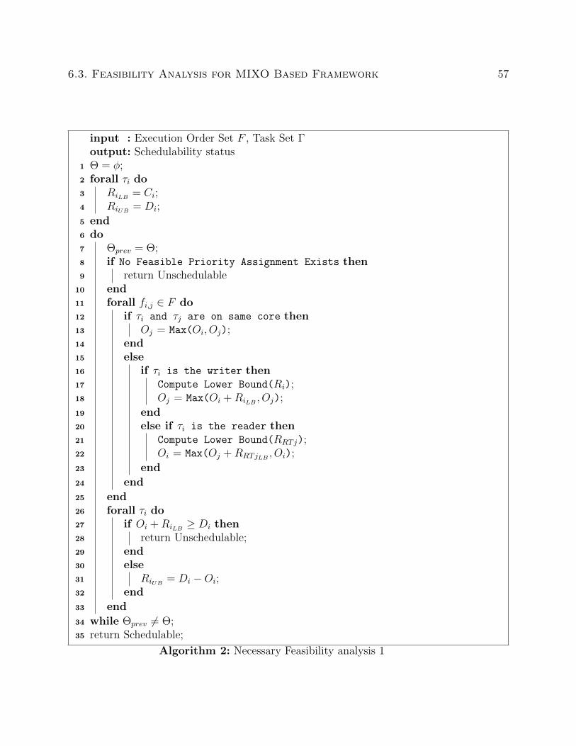
6.3. Feasibility Analysis for MIXO Based Framework 57
input : Execution Order Set F , Task Set Γoutput: Schedulability status
1 Θ = φ;2 forall τi do3 RiLB
= Ci;4 RiUB
= Di;
5 end6 do7 Θprev = Θ;8 if No Feasible Priority Assignment Exists then9 return Unschedulable
10 end11 forall fi,j ∈ F do12 if τi and τj are on same core then13 Oj = Max(Oi, Oj);14 end15 else16 if τi is the writer then17 Compute Lower Bound(Ri);18 Oj = Max(Oi +RiLB
, Oj);
19 end20 else if τi is the reader then21 Compute Lower Bound(RRTj);22 Oi = Max(Oj +RRTjLB
, Oi);
23 end
24 end
25 end26 forall τi do27 if Oi +RiLB
≥ Di then28 return Unschedulable;29 end30 else31 RiUB
= Di −Oi;32 end
33 end
34 while Θprev 6= Θ;35 return Schedulable;
Algorithm 2: Necessary Feasibility analysis 1

58 Chapter 6. Customized Optimization Algorithm
Thus we say that the system is not F -feasible.
However, F1 = {f3,0} makes Γ F1-feasible. The design constraint imposed is
O0 = maxO0, O3 +RRT3LB(6.19)
By Lines 17 and 21, we compute lower bound response time values with no partial priority
order constraints as
[R0LBRRT3LB
] = [20, 10] (6.20)
By Line 18 and equation (6.19), we compute the lowest bound offset values [O0, O3] = [10, 0]
We see that R0LB+ O0 ≤ D0 with a feasible priority assignment p0 > p1, p2 > p3. Upon re-
iterating, we see that the computed offset values do not change. Thus, we say that the system
is F1-feasible as there exists a feasible priority assignment and the system is schedulable for
the lowest possible response time and offset assignment.
Even though this analysis cannot compute all MIXOs as it optimistically checks for feasibility,
it helps in computing obviously infeasible execution orders before exact analysis can be
used. Furthermore, we observe that the basic feasibility analysis for both exact analysis and
necessary analysis 1, involves checking if a feasible priority assignment exists. Thus for an
even more primitive analysis we can check if a feasible priority assignment exists before using
the above mentioned necessary analysis 1 or the exact analysis.
6.3.3 Necessary Feasibility Analysis 2
In this feasibility analysis, we further simplify the feasibility condition to simply determine
if a feasible priority assignment exists. In this feasibility test we do not consider offset
assignment but rather just check if the partial priority order enforced by F can return a
feasible priority assignment. To determine if such a priority assignment exists we simply use
6.3. Feasibility Analysis for MIXO Based Framework 59
a revised version of Audsley’s algorithm as mentioned in exact feasibility analysis (mentioned
in section 6.3.1). We compute this assignment, by iteratively assigning priorities to tasks
starting with lowest priority first, such that (a) the response time of tasks does not exceed
their deadlines and (b) the partial priority order satisfies constraints (6.9) imposed by the
execution order. Since this analysis considers only restrictions for intra-core links, it is quite
fast as compared to necessary analysis 1 and the exact analysis. However, this also means
that it is the most flexible test and hence will fail to find as many MIXOs as necessary
analysis 1 or exact analysis.
6.3.4 Final Algorithm for Feasibility Analysis
For developing an efficient dedicated algorithm for feasibility analysis we use all the afore-
mentioned schedulability tests in a cascaded form as shown in Figure 6.3 (Steps 3-5). We
start with necessary analysis 2 to check if a feasible priority assignment exists. If Γ is not
F -feasible at this level, we say that a feasible priority assignment does not exist for the given
execution order set, and hence we compute MIXO accordingly. If F passes the feasibility test
using necessary analysis 2, we use necessary analysis 1 for a stricter feasibility test. Finally
if the system is F -feasible for both necessary analysis, we use exact analysis for a complete
feasibility test. By using this multi-layered approach, we see that the necessary analysis 1
and 2 shape the majority of the schedulability region of the MILP and thus significantly
reduce the computation load on exact analysis. Since using exact analysis itself is more ef-
ficient than MILP formulation [51], using this multi-layered approach guarantees to provide
a much better run-time as compared to using MILP formulation.

60 Chapter 6. Customized Optimization Algorithm
Solve MILP formula�on ∏ with CPLEX
Feasible?No
Yes
Start with MILP formula�on ∏ without any constraint on F-feasibility
Use necessary analysis 2 for F-feasibility Step 3
Feasible?No
Yes
Par�al execu�on order set F*
Add MIXO-implied
constraints to ∏
Report op�mal execu�on order
Step 2
Step 1
Use necessary analysis 1 for F-feasibility Step 4
Compute k MIXOs using
Algorithm 1
Compute k MIXOs using
Algorithm 1
Feasible?
Yes
NoReport infeasibility
Step 6
Feasible?No
Yes
Use exact analysis for F-feasibility Step 5
Compute k MIXOs using
Algorithm 1
Figure 6.3: MIXO-guided Framework
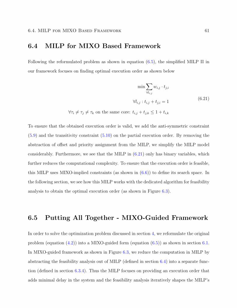
6.4. MILP for MIXO Based Framework 61
6.4 MILP for MIXO Based Framework
Following the reformulated problem as shown in equation (6.5), the simplified MILP Π in
our framework focuses on finding optimal execution order as shown below
min∑∀li,j
wi,j · tj,i
∀li,j : ti,j + tj,i = 1
∀τi 6= τj 6= τk on the same core: ti,j + tj,k ≤ 1 + ti,k
(6.21)
To ensure that the obtained execution order is valid, we add the anti-symmetric constraint
(5.9) and the transitivity constraint (5.10) on the partial execution order. By removing the
abstraction of offset and priority assignment from the MILP, we simplify the MILP model
considerably. Furthermore, we see that the MILP in (6.21) only has binary variables, which
further reduces the computational complexity. To ensure that the execution order is feasible,
this MILP uses MIXO-implied constraints (as shown in (6.6)) to define its search space. In
the following section, we see how this MILP works with the dedicated algorithm for feasibility
analysis to obtain the optimal execution order (as shown in Figure 6.3).
6.5 Putting All Together - MIXO-Guided Framework
In order to solve the optimization problem discussed in section 4, we reformulate the original
problem (equation (4.2)) into a MIXO-guided form (equation (6.5)) as shown in section 6.1.
In MIXO-guided framework as shown in Figure 6.3, we reduce the computation in MILP by
abstracting the feasibility analysis out of MILP (defined in section 6.4) into a separate func-
tion (defined in section 6.3.4). Thus the MILP focuses on providing an execution order that
adds minimal delay in the system and the feasibility analysis iteratively shapes the MILP’s

62 Chapter 6. Customized Optimization Algorithm
feasibility region using MIXO-implied constraints. One issue of designing a framework based
on MIXO-implied constraint (6.6) for modeling the feasibility regions is that the total number
of MIXOs grows exponentially w.r.t. the size of the system. For example, for a system with
m communication links, which suggests 2m partial execution orders necessary to consider,
the total number of MIXOs can be O(22m). Modeling the entire feasibility region would
need to enumerate all MIXOs and their implied constraints, which is obviously impractical
for large systems. However, this is rarely necessary. We observe that in most cases, the
optimization objective is only sensitive to a small number of MIXOs. Thus, we propose an
iterative refinement procedure that selectively explores and adds MIXO-implied constraints
guided by the optimization objective, i.e., to derive and enforce MIXO-implied constraints
only when the optimization algorithm returns infeasible solutions (i.e., the returned partial
execution order set is infeasible). The framework works by iterating through the below steps
till the MILP provides an execution order that passes all the levels of feasibility analysis.
Step 1: Start with no schedulability constraints: We define the problem as done in section
6.1 with no initial constraints for feasibility of the execution order.
Step 2: Solving the MILP Π: To do so, we use the MILP defined in section 6.4. This
MILP returns an execution order set F ∗ which adds minimal delay in the system such that
F ∗ = {fi,j|ti,j = 1}. However, if no such execution order exists i.e. if the MILP cannot find
a feasible solution, we return that the system is infeasible. This might happen during the
run-time, if the utilization is too high to obtain any feasible priority assignment.
Step 3: Use Necessary Analysis 2: In this step we confirm if a feasible priority assignment
exists for the computed execution order. Otherwise, we compute k MIXOs that are added as
constraints back to the MILP. To limit the run-time of each iteration, we allow a maximum of
5 schedulability constraints to be computed for a given execution order set. If the execution
order is feasible for necessary analysis 2, we move to Step 4
Step 4: Using Necessary Analysis 1: Similar to Step 3, we use necessary analysis to check if

6.5. Putting All Together - MIXO-Guided Framework 63
the execution order is feasible. If it is feasible we continue to Step 5, otherwise we compute
the corresponding MIXO-implied constraints to be added to the MILP.
Step 5: Using Exact Analysis: Since the execution order is feasible for both necessary anal-
ysis 1 and 2, we do a complete feasibility test using exact feasibility analysis. In case of
infeasibility, MIXOs are computed and added as constraints to MILP. Otherwise, we return
that the obtained execution order is optimal.
Step 6: Adding MIXO-implied constraints: In this step, we add MIXO-implied constraints
as shown in equation (6.6) to shape the feasibility region of the MILP.
Thus by iterating through the above mentioned steps, we compute the optimal execution
order for a given system. Furthermore, as seen from section 4, once we obtain the optimal
execution order we can iterate through its elements and find the corresponding minimal delay
block assignment.
Remark 6.12. In Step 2, it is possible that problem Π becomes infeasible at some point.
This happens for example, when the utilization of the system is so high that no priority
assignment can schedule it. In this case, given any partial execution order set F , Algorithm 1
always returns F = ∅. The MIXO-implied by an empty set would be 0 ≤ −1, which causes
Π to be infeasible.
The algorithm is also guaranteed to terminate. This is because the number of MIXOs is
finite, and during each iteration between Steps 2–6, the algorithm will find new MIXOs that
are different from known ones. Finally, if a solution is deemed feasible at Step 5, it must
be optimal with respect to the original problem, as it is optimal to a relaxed problem Π: Π
only includes the implied constraints of a subset of all MIXOs.
We can see the working of this framework from the example below.
Example 6.13. We consider the system Γ shown in Fig 6.1 with the assumption that the
cost of delay block addition on all links is 1 i.e. ∀li,j : wi,j = 1 . We now see, how our

64 Chapter 6. Customized Optimization Algorithm
MIXO-guided framework solves the problem of optimal execution order for Γ.
Iteration 1 : Step 1 :We first initialize the problem into the problem of finding an optimal
execution order as shown below:
min t1,0 + t3,0 + t2,1 + t2,3
s.t. Γ is F -feasible
where F = {fi,j|ti,j = 1}
(6.22)
Step 2 : We formulate the MILP Π as shown in (6.23)
min t1,0 + t3,0 + t2,1 + t2,3
∀li,j : ti,j + tj,i = 1
(6.23)
Solving Π returns the execution order F ∗ = {f0,1, f0,3, f1,2, f3,2}
Step 3 : The system Γ is not F ∗-feasible for necessary analysis 2, as a feasible priority
assignment is not possible with partial priority order P3,2 = 1. Thus we compute the MIXO
U1 = {f3,2} using algorithm 1
Step 6: We use the computed U to add the schedulability constraint as shown below.
t3,2 ≤ 0 (6.24)
Iteration 2: Step 2: We solve the MILP (6.23) with constraint (6.24) and thus get the
following solution F ∗ = {f0,1, f0,3, f1,2, f2,3}
Step 3: We see that Γ is F ∗-feasible for necessary analysis 2 as a feasible priority assignment
p0 > p1, p2 > p3 that satisfies the design constraints imposed by F ∗.
Step 4: We see that the system is not F ∗-feasible by using necessary analysis 1 (as shown in
example 6.11). The computed MIXOs are U2 = {f0,3} and U3 = {f1,2}

6.5. Putting All Together - MIXO-Guided Framework 65
Step 6: The schedulability constraints thus computed from U2 and U3 are
t1,2 ≤ 0
t0,3 ≤ 0
(6.25)
Iteration 3: Step 2: We solve MILP (6.23) with constraints (6.24) and (6.25) thus giving
us the solution F ∗ = {f0,1, f3,0, f2,1, f2,3}.
Step 3: We see that Γ is F ∗-feasible for necessary analysis 2
Step 4: We see that Γ is F ∗-feasible for necessary analysis 1 as the system is schedulable
with the computed lowest possible offset assignment and response time.
Step 5: We see that Γ is F ∗-feasible (as shown in example 6.10). Thus we say that F ∗ is the
optimal execution order for our system Γ.
We can now determine the delay block assignment from the obtained F by using principles
1, 2, 3 and 4. Thus iterating for each element in F , we get the delay block assignment as
DB0,1 = 0, DB1,2 = 1, DB0,3 = 1, DB3,2 = 1.

Chapter 7
Results
In this section, we present the results of our experimental evaluation. We compare be-
tween the proposed MIXO-guided optimization framework and the MILP solution. Our
experiments consists of two parts. The first evaluates on randomly generated systems with
different settings and the second evaluates on an industrial case study of fuel injection sys-
tem. The two techniques are compared in terms of run-time and the number of unit delay
blocks added.
7.1 Experiment on Random Systems
This experiment aims to evaluate the performance of MIXO-guided optimization and MILP
for systems across a wide range of settings. The first part of the experiment evaluates w.r.t
systems of different number of tasks. We use Task Graphs For Free (TGFF) [19] for generat-
ing random acyclic directed graphs. The maximum number of writers to each task is limited
to 3 and the maximum number of readers are 2. We consider dual-core platform (2 proces-
sors). System total utilization is randomly selected from interval [1.4, 1.8]. Number of tasks
varies from 10 to 70, which are then randomly and evenly distributed to the two processors.
Utilization of each task is generated using UUnifast-Discard algorithm [14]. Periods are
randomly chosen from a predefined set of values {5, 10, 20, 40, 50, 100, 200, 400, 500, 1000},
which contains all the periods for the real-world automotive benchmark in [29]. To avoid
excessive waiting time on difficult systems, we set a time limit of 30min for both techniques.
66

7.1. Experiment on Random Systems 67
10 20 30 40 50 60 70
0
500
1,000
1,500
Number of tasks
RunT
ime
(in
sec)
MILPMIXO-guided
Figure 7.1: Average Run-Time for 1000 Random Systems
The average run-time by the two techniques is summarized in Figure 7.1. Each data point
in the figure represents the average out of 1000 randomly generated systems. For systems
with up to 50 tasks, MIXO-guided optimization and MILP have comparable performance.
However, for larger systems comprising of 60 and more tasks, the complexity of MILP
drastically increases. MIXO-guided optimization technique proves to 10X faster than MILP
for 60-task systems. Furthermore, for 70-task systems, MILP timeouts for 65% of cases
while MIXO-guided optimization technique only timeouts for 6%. Thus, we can see that
the proposed MIXO-guided framework is more scalable than MILP.
We then fix the total number of tasks to be 50, and check how the runtime of the algorithms
vary with respect to a given system utilization. Hence, we fix the system utilization to
be 1.2 to 1.8, and collect the average runtime of both algorithms. Figure 7.2 illustrates
the results. As in the figure, MIXO-guided framework always runs faster than MILP, and
the gap in their algorithm efficiency becomes larger for higher utilization: at 180% system
utilization (averagely 90% on each core), MIXO-guided is about 15 times faster than MILP.
As mentioned in section 6.3, the primary reason that MIXO-guided framework performs

68 Chapter 7. Results
1.2 1.3 1.4 1.5 1.6 1.7 1.80
20
40
60
80
100
120
Utilization Value
RunT
ime
(in
sec)
MILPMIXO-guided
Figure 7.2: Average Run-Time for 50 tasks vs Utilization
Analysis % of MIXOs computed Time to compute single MIXOExact Analysis 22 % 1.145 sec
Necessary Analysis 1 37 % 0.014 secNecessary Analysis 2 41 % 0.08 sec
Table 7.1: Comparing performance of each Analysis
better is that we shift the feasibility analysis into a much more efficient algorithm. We can
see that our dedicated algorithm for feasibility analysis performs much better than using
MILP formulation from the results obtained in Table 7.1 for 50 tasks. As mentioned in
[51], the exact analysis itself is much faster than the MILP formulation. Furthermore, the
results from Table 7.1 shows that the necessary analysis 1 and necessary analysis 2 perform
upto 2 orders of magnitude faster than the exact analysis. At the same time, cumulatively
they shape 78% of the feasibility region with their computed MIXOs, before shifting to the
exact analysis. Thus, we can see that using the faster approximate analysis to compute
the majority of MIXOs before the expensive exact analysis (as shown in Figure 6.3) greatly
improves our run-time performance compared to MILP.

7.1. Experiment on Random Systems 69
10 20 30 40 50 60 70
0.25
0.3
0.35
0.4
0.45
Number of tasks
Del
ay/
Tot
alL
inks
MILPMIXO-guided
Figure 7.3: Normalized Objective Analysis for 1000 Random systems
Next we compare the average normalized objective by the two techniques. The normalized
objective is defined as the objective value (the minimum number of unit delay RT blocks)
over the total number of communication links. Two special cases need to be considered.
If a technique fails to find any solution within the time limit, we consider the normalized
objective to be 1 as a penalty. If a technique is capable of detecting infeasibility within the
time limit, we consider the normalized objective to be 0. Intuitively, the average normalized
objective reflects the optimization quality of an algorithm. The results are summarized in
Figure 7.3. The two techniques perform comparably for small systems of no larger than 50
tasks. For larger system of 60 and more tasks, MIXO-guided technique gives much better
optimization result than MILP. This is mainly due to a large number of cases where MILP
either timeouts without finding any feasible solutions or finding only sub-optimal solutions.
The results of these experiments on random systems can be seen in a tabular form in Table
7.2.

70 Chapter 7. Results
TaskCount
Average Run-Time (in sec) Average Normalized Objective Total TimeoutsMILP MIXO-guided MILP MIXO-guided MILP MIXO-guided
10 0.003 0.001 0.35 0.35 0 020 0.047 0.023 0.28 0.28 0 030 0.51 0.2 0.25 0.25 0 040 7.62 1.72 0.243 0.243 1 050 84.42 12.811 0.238 0.235 10 060 647.86 67.945 0.296 0.223 180 170 1430.97 348.7 0.45 0.30 651 62
Table 7.2: Results for 1000 Random Systems
7.2 Fuel Injection System Case Study
Our second experiment evaluates on an industrial case study of a simplified fuel-injection
system [18]. The system contains 90 tasks with 106 communication links. The case study
was originally configured to run on a single core platform. Thus we modify the case study
for use on a dual-core system. Specifically, we scale the WCET of each task to reach a total
utilization of 1.9 (Averagely 95% for each processor). We apply both the MILP as well as
the MIXO-guided optimization to optimize the case study system. We consider various task
partition schemes on the two cores to obtain the results as shown in Table 7.3. The first
column shows the number of tasks allocated to core 0 and the second column shows the
number of tasks allocated to core 1.
While both are capable of terminating and finding the same optimal solution, the MIXO-
guided optimization technique is 2 to 3 magnitudes faster than MILP. Furthermore, MIXO-
based approach remains consistent with the varying partitioning scheme, whereas the MILP’s
complexity drastically increases with more number of tasks on a single core. It is also
interesting to note that although the size of the fuel injection case study is larger than
the randomly generated systems in the previous experiment, the performance of MIXO-
guided algorithm is much better. This is mainly due to the following characteristics of the
case study: (i) The total utilization of the case study is very high, almost approaching the

7.2. Fuel Injection System Case Study 71
Task Count Run TimeObjective Utilization
Core 0 Core 1 MILP MIXO-guided90 0 25 hrs 2 min 5.15 sec 21 0.9480 10 3 hrs 10 min 8.45 sec 21 1.9070 20 1 hr 18 min 6.11 sec 21 1.9060 30 26 min 45 sec 6.38 sec 21 1.9045 45 19 min 4 sec 7.7 sec 21 1.90
Table 7.3: Results for Fuel-Injection Case Study
limit that allows schedulability; (ii) For many of the low rate to high rate communication
links li,j, the periods of the reader and writer are drastically different (e.g., a 1Hz block
communicating to a 250Hz block). Since the WCETs of blocks are roughly proportional
to their periods, enforcing a partial execution order for these links where the lower rate
task executes first would easily cause system unschedulability. As a result, for many of
the low rate to high rate communication links, there is only one possible partial execution
order that may be enforced. For other high rate to low rate communications li,j, enforcing
fi,j is typically the optimal decision as it mostly helps schedulability without having to
introduce unit delay blocks. The proposed MIXO-guided optimization technique readily
exploits such characteristics. Specifically, since it starts with an overapproximation of the
feasibility region (the constraints on F -feasibility is initially omitted), it naturally attempts
to enforce fi,j for all communication links li,j, which is typically optimal for high rate to
low rate communication. For low rate to high rate communication li,j, the fact that many
of them have only one feasible execution order would lead the algorithm to compute lots
of MIXOs that contains only one element (i.e., U = {fi,j}). The implied constraint of
such one-element MIXO essentially fixes the value on the variable li,j. This quickly leads the
algorithm to reduce the search space and identify the optimal solution. Such problem-specific
optimization structure appears to be more difficult to exploit in standard MILP.

Chapter 8
Conclusion and Future Work
In this thesis, we consider the problem of software synthesis for Simulink models on multicore
architectures with partitioned fixedpriority scheduling. We consider a mechanism for seman-
tics preservation on such platforms, that assigns task offsets and leverages the Simulink RT
blocks. This avoids accessing the global shared variables at the same time from the writer
and reader on different cores, and enforces a proper execution order between them. We
propose to optimize the cost associated to the unit delay RT block, and present two ap-
proaches. One is a direct MILP formulation, the other is a customized exact procedure. Our
evaluation on random system shows that for small systems of size less than 50 tasks, the two
algorithms performs comparably well. For larger systems however, our customized exact pro-
cedure algorithm is much more scalable. For randomly generated systems, our customized
procedure runs 10X faster and gives significantly better optimization quality comparing to
MILP. Our evaluation on industrial case study also demonstrates its potential for handling
large scale real-world problems efficiently as it performs upto four orders of magnitude faster
than MILP. Furthermore, our framework shows consistent performance for varying utiliza-
tion and partitioning schemes, whereas MILP on the other hand shows strong variations.
For future work, we plan to include task-to-core allocation into the design space to further
improve the solution quality. Furthermore, we seek to include the mapping of blocks to tasks
as well to further optimize the generated software quality. To get a more accurate estimate
on the improvement in performance, we seek to implement this on a hardware platform in
the future (like Kalray 256).
72

Bibliography
[1] Analytics. URL https://www.ibm.com/analytics/data-science/
prescriptive-analytics/cplex-optimizer.
[2] Zaid Al-bayati, Haibo Zeng, Marco Di Natale, and Zonghua Gu. Multitask implemen-
tation of synchronous reactive models with earliest deadline first scheduling. In IEEE
International Symposium on Industrial Embedded Systems, 2013.
[3] Sebastian Altmeyer, Robert I. Davis, Leandro Indrusiak, Claire Maiza, Vincent Nelis,
and Jan Reineke. A generic and compositional framework for multicore response time
analysis. In Proceedings of the 23rd International Conference on Real Time and Net-
works Systems, RTNS ’15, pages 129–138, New York, NY, USA, 2015. ACM. ISBN 978-
1-4503-3591-1. doi: 10.1145/2834848.2834862. URL http://doi.acm.org/10.1145/
2834848.2834862.
[4] N. C. Audsley. On priority asignment in fixed priority scheduling. Inf. Process. Lett.,
79(1):39–44, May 2001. ISSN 0020-0190. doi: 10.1016/S0020-0190(00)00165-4. URL
http://dx.doi.org/10.1016/S0020-0190(00)00165-4.
[5] Philip Axer, Rolf Ernst, Heiko Falk, Alain Girault, Daniel Grund, Nan Guan, Bengt
Jonsson, Peter Marwedel, Jan Reineke, Christine Rochange, Maurice Sebastian, Rein-
hard Von Hanxleden, Reinhard Wilhelm, and Wang Yi. Building timing predictable
embedded systems. ACM Trans. Embed. Comput. Syst., 13(4):82:1–82:37, March 2014.
ISSN 1539-9087. doi: 10.1145/2560033. URL http://doi.acm.org/10.1145/2560033.
[6] Gerard Berry and Georges Gonthier. The esterel synchronous programming language:
Design, semantics, implementation. Sci. Comput. Program., 19(2):87–152, November
73

74 BIBLIOGRAPHY
1992. ISSN 0167-6423. doi: 10.1016/0167-6423(92)90005-V. URL http://dx.doi.
org/10.1016/0167-6423(92)90005-V.
[7] Dai Bui, Edward Lee, Isaac Liu, Hiren Patel, and Jan Reineke. Temporal isolation on
multiprocessing architectures. In Proceedings of the 48th Design Automation Confer-
ence, DAC ’11, pages 274–279, New York, NY, USA, 2011. ACM. ISBN 978-1-4503-
0636-2. doi: 10.1145/2024724.2024787. URL http://doi.acm.org/10.1145/2024724.
2024787.
[8] Thomas Carle, Dumitru Potop-Butucaru, Yves Sorel, and David Lesens. From dataflow
specification to multiprocessor partitioned time-triggered real-time implementation.
Leibniz Transactions on Embedded Systems, 2(2):01–1–01:30, 2015. ISSN 2199-2002. doi:
10.4230/LITES-v002-i002-a001. URL https://ojs.dagstuhl.de/index.php/lites/
article/view/LITES-v002-i002-a001.
[9] P. Caspi, N. Scaife, C. Sofronis, and S. Tripakis. Semantics-preserving multitask im-
plementation of synchronous programs. ACM Trans. Embed. Comput. Syst., 7(2):1–40,
2008.
[10] Paul Caspi and Albert Benveniste. Time-robust discrete control over networked loosely
time-triggered architectures. In IEEE Conf. Decision & Control, 2008.
[11] Paul Caspi, Adrian Curic, Aude Maignan, Christos Sofronis, Stavros Tripakis, and
Peter Niebert. From simulink to scade/lustre to tta: A layered approach for distributed
embedded applications. In ACM Conference on Language, Compiler, and Tool for
Embedded Systems, 2003.
[12] Paul Caspi, Norman Scaife, Christos Sofronis, and Stavros Tripakis. Semantics-
preserving multitask implementation of synchronous programs. ACM Transactions on
Embedded Computing Systems (TECS), 7(2):15, 2008.

BIBLIOGRAPHY 75
[13] J. Chen and A. Burns. Loop-free asynchronous data sharing in multiprocessor real-time
systems based on timing properties. In IEEE Conference on Real-Time Computing
Systems and Applications, 1999.
[14] Robert I Davis and Alan Burns. Priority assignment for global fixed priority pre-emptive
scheduling in multiprocessor real-time systems. In Real-Time Systems Symposium, 2009,
RTSS 2009. 30th IEEE, pages 398–409. IEEE, 2009.
[15] Robert I. Davis, Sebastian Altmeyer, Leandro Indrusiak, Claire Maiza, Vincent Nelis,
and Jan Reineke. An extensible framework for multicore response time analysis. Real-
Time Systems, 2017.
[16] Marco Di Natale and Valerio Pappalardo. Buffer optimization in multitask implemen-
tations of simulink models. ACM Transactions on Embedded Computing Systems, 7(3):
23, 2008.
[17] Marco Di Natale, Liangpeng Guo, Haibo Zeng, and Alberto Sangiovanni-Vincentelli.
Synthesis of multitask implementations of simulink models with minimum delays. IEEE
Transactions on Industrial Informatics, 6(4):637–651, 2010.
[18] Marco Di Natale, Liangpeng Guo, Haibo Zeng, and Alberto Sangiovanni-Vincentelli.
Synthesis of multitask implementations of simulink models with minimum delays. In-
dustrial Informatics, IEEE Transactions on, 6(4):637–651, 2010.
[19] R. P. Dick, D. L. Rhodes, and W. Wolf. Tgff: task graphs for free. In Hardware/Software
Codesign, 1998. (CODES/CASHE ’98) Proceedings of the Sixth International Workshop
on, pages 97–101, Mar 1998. doi: 10.1109/HSC.1998.666245.
[20] Guy Durrieu, Madeleine Faugere, Sylvain Girbal, Daniel Gracia Perez, Claire Pagetti,
and W. Puffitsch. Predictable Flight Management System Implementation on a Mul-

76 BIBLIOGRAPHY
ticore Processor. In Embedded Real Time Software (ERTS’14), TOULOUSE, France,
February 2014. URL https://hal.archives-ouvertes.fr/hal-01121700.
[21] J. Forget, F. Boniol, D. Lesens, and C. Pagetti. A multi-periodic synchronous data-flow
language. In IEEE High Assurance Systems Engineering Symposium, Dec 2008.
[22] J. Forget, F. Boniol, and C. Pagetti. Verifying end-to-end real-time constraints on multi-
periodic models. In 2017 22nd IEEE International Conference on Emerging Technologies
and Factory Automation (ETFA), pages 1–8, Sept 2017. doi: 10.1109/ETFA.2017.
8247612.
[23] Amaury Graillat, Matthieu Moy, Pascal Raymond, and Benoıt Dupont De Dinechin.
Parallel Code Generation of Synchronous Programs for a Many-core Architecture. In
Design, Automation and Test in Europe, 2018.
[24] Nicholas Halbwachs, Paul Caspi, Pascal Raymond, and Daniel Pilaud. The synchronous
data flow programming language lustre. Proceedings of the IEEE, 79(9):1305–1320, 1991.
[25] G. Han, H. Zeng, M. Di Natale, X. Liu, and W. Dou. Experimental evaluation and
selection of data consistency mechanisms for hard real-time applications on multicore
platforms. IEEE Transactions on Industrial Informatics, 10(2):903–918, May 2014.
ISSN 1551-3203. doi: 10.1109/TII.2013.2290585.
[26] Donghyun Kang, Junchul Choi, and Soonhoi Ha. Worst case delay analysis of shared
resource access in partitioned multi-core systems. In Proceedings of the 15th IEEE/ACM
Symposium on Embedded Systems for Real-Time Multimedia, ESTIMedia ’17, pages 84–
92, New York, NY, USA, 2017. ACM. ISBN 978-1-4503-5117-1. doi: 10.1145/3139315.
3139322. URL http://doi.acm.org/10.1145/3139315.3139322.
[27] Timon Kelter and Peter Marwedel. Parallelism analysis: Precise wcet values for complex

BIBLIOGRAPHY 77
multi-core systems. In Cyrille Artho and Peter Csaba Olveczky, editors, Formal Tech-
niques for Safety-Critical Systems, pages 142–158, Cham, 2015. Springer International
Publishing. ISBN 978-3-319-17581-2.
[28] Enagnon Cedric Klikpo and Alix Munier-Kordon. Preemptive scheduling of dependent
periodic tasks modeled by synchronous dataflow graphs. In Proceedings of the 24th
International Conference on Real-Time Networks and Systems, RTNS ’16, pages 77–86,
New York, NY, USA, 2016. ACM. ISBN 978-1-4503-4787-7. doi: 10.1145/2997465.
2997474. URL http://doi.acm.org/10.1145/2997465.2997474.
[29] Simon Kramer, Dirk Ziegenbein, and Arne Hamann. Real world automotive bench-
marks for free. In 6th International Workshop on Analysis Tools and Methodologies for
Embedded and Real-time Systems (WATERS), 2015.
[30] Claudio Maia, Marko Bertogna, Luıs Nogueira, and Luis Miguel Pinho. Response-time
analysis of synchronous parallel tasks in multiprocessor systems. In Proceedings of the
22Nd International Conference on Real-Time Networks and Systems, RTNS ’14, pages
3:3–3:12, New York, NY, USA, 2014. ACM. ISBN 978-1-4503-2727-5. doi: 10.1145/
2659787.2659815. URL http://doi.acm.org/10.1145/2659787.2659815.
[31] Leonardo Mangeruca, Massimo Baleani, Alberto Ferrari, and Alberto Sangiovanni-
Vincentelli. Uniprocessor scheduling under precedence constraints for embedded systems
design. ACM Transactions on Embedded Computing Systems, 7(1):6, 2007.
[32] Sebastien Martinez, Damien Hardy, and Isabelle Puaut. Quantifying wcet reduction of
parallel applications by introducing slack time to limit resource contention. In Proceed-
ings of the 25th International Conference on Real-Time Networks and Systems, RTNS
’17, pages 188–197, New York, NY, USA, 2017. ACM. ISBN 978-1-4503-5286-4. doi:
10.1145/3139258.3139263. URL http://doi.acm.org/10.1145/3139258.3139263.
78 BIBLIOGRAPHY
[33] Vincent Nelis, Patrick Meumeu Yomsi, and Luıs Miguel Pinho. The Variability of
Application Execution Times on a Multi-Core Platform. In Martin Schoeberl, editor,
16th International Workshop on Worst-Case Execution Time Analysis (WCET 2016),
volume 55 of OpenAccess Series in Informatics (OASIcs), pages 6:1–6:11, Dagstuhl,
Germany, 2016. Schloss Dagstuhl–Leibniz-Zentrum fuer Informatik. ISBN 978-3-95977-
025-5. doi: 10.4230/OASIcs.WCET.2016.6. URL http://drops.dagstuhl.de/opus/
volltexte/2016/6899.
[34] Haluk Ozaktas, Christine Rochange, and Pascal Sainrat. Minimizing the cost of syn-
chronisations in the wcet of real-time parallel programs. In Proceedings of the 17th
International Workshop on Software and Compilers for Embedded Systems, SCOPES
’14, pages 98–107, New York, NY, USA, 2014. ACM. ISBN 978-1-4503-2941-5. doi:
10.1145/2609248.2609261. URL http://doi.acm.org/10.1145/2609248.2609261.
[35] Claire Pagetti, Julien Forget, Frederic Boniol, Mikel Cordovilla, and David Lesens.
Multi-task implementation of multi-periodic synchronous programs. Discrete event dy-
namic systems, 21(3):307–338, 2011.
[36] Claire Pagetti, David Saussie, Romain Gratia, Eric Noulard, and Pierre Siron. The
ROSACE case study: From simulink specification to multi/many-core execution. In
IEEE Real-Time and Embedded Technology and Applications Symposium, 2014.
[37] Q. Perret, P. Maurere, E. Noulard, C. Pagetti, P. Sainrat, and B. Triquet. Temporal
isolation of hard real-time applications on many-core processors. In 2016 IEEE Real-
Time and Embedded Technology and Applications Symposium (RTAS), pages 1–11, April
2016. doi: 10.1109/RTAS.2016.7461363.
[38] D. Potop-Butucaru, B. Caillaud, and A. Benveniste. Concurrency in synchronous sys-
tems. In Int. Conf. Application of Concurrency to System Design, 2004.

BIBLIOGRAPHY 79
[39] D. Potop-Butucaru, S. A. Edwards, and G. Berry. Compiling Esterel. Springer, 2007.
[40] Dumitru Potop-Butucaru and Isabelle Puaut. Integrated Worst-Case Execution Time
Estimation of Multicore Applications. In Claire Maiza, editor, 13th International Work-
shop on Worst-Case Execution Time Analysis, volume 30 of OpenAccess Series in In-
formatics (OASIcs), pages 21–31, Dagstuhl, Germany, 2013. Schloss Dagstuhl–Leibniz-
Zentrum fuer Informatik. ISBN 978-3-939897-54-5. doi: 10.4230/OASIcs.WCET.2013.
21. URL http://drops.dagstuhl.de/opus/volltexte/2013/4119.
[41] Claudius Ptolemaeus, editor. System Design, Modeling, and Simulation using Ptolemy
II. Ptolemy.org, 2014. URL http://ptolemy.org/books/Systems.
[42] W. Puffitsch, E. Noulard, and C. Pagetti. Mapping a multi-rate synchronous language to
a many-core processor. In IEEE Real-Time and Embedded Technology and Applications
Symposium, April 2013.
[43] Wolfgang Puffitsch, Eric Noulard, and Claire Pagetti. Off-line mapping of multi-rate
dependent task sets to many-core platforms. Real-Time Systems, 51(5):526–565, 2015.
[44] Hamza Rihani, Matthieu Moy, Claire Maiza, Robert I. Davis, and Sebastian Altmeyer.
Response Time Analysis of Synchronous Data Flow Programs on a Many-Core Proces-
sor. In RTNS 2016, 24th International Conference on Real-Time Networks and Systems,
Brest, France, Oct 2016.
[45] The MathWorks. The mathworks simulink and stateflow user’s manuals. web page:
http://www.mathworks.com.
[46] S. Tripakis, C. Pinello, A. Benveniste, A. Sangiovanni-Vincent, P. Caspi, and M. Di
Natale. Implementing synchronous models on loosely time triggered architectures. IEEE
Transactions on Computers, 57(10):1300–1314, Oct 2008.
80 BIBLIOGRAPHY
[47] Stavros Tripakis, Christos Sofronis, Paul Caspi, and Adrian Curic. Translating discrete-
time simulink to lustre. ACM Transactions on Embedded Computing Systems (TECS),
4(4):779–818, 2005.
[48] Simon Wegener. Towards Multicore WCET Analysis. In Jan Reineke, editor, 17th Inter-
national Workshop on Worst-Case Execution Time Analysis (WCET 2017), volume 57
of OpenAccess Series in Informatics (OASIcs), pages 7:1–7:12, Dagstuhl, Germany,
2017. Schloss Dagstuhl–Leibniz-Zentrum fuer Informatik. ISBN 978-3-95977-057-6. doi:
10.4230/OASIcs.WCET.2017.7. URL http://drops.dagstuhl.de/opus/volltexte/
2017/7311.
[49] Haibo Zeng and Marco Di Natale. Mechanisms for guaranteeing data consistency and
flow preservation in autosar software on multi-core platforms. In IEEE International
Symposium on Industrial Embedded Systems, 2011.
[50] Haibo Zeng and Marco Di Natale. Mechanisms for guaranteeing data consistency and
flow preservation in autosar software on multi-core platforms. In 6th IEEE International
Symposium on Industrial Embedded Systems, pages 140–149, 2011.
[51] Y. Zhao and H. Zeng. The virtual deadline based optimization algorithm for priority
assignment in fixed-priority scheduling. In 2017 IEEE Real-Time Systems Symposium
(RTSS), volume 00, pages 116–127, Dec 2017. doi: 10.1109/RTSS.2017.00018. URL
doi.ieeecomputersociety.org/10.1109/RTSS.2017.00018.
[52] Yecheng Zhao and Haibo Zeng. The concept of unschedulability core for optimizing
priority assignment in real-time systems. In Proceedings of the Conference on De-
sign, Automation & Test in Europe, DATE ’17, pages 232–237, 3001 Leuven, Bel-
gium, Belgium, 2017. European Design and Automation Association. URL http:
//dl.acm.org/citation.cfm?id=3130379.3130432.