Optimal Income Taxation:Mirrlees Meets Ramsey

Jonathan HeathcoteFRB Minneapolis and CEPR

Hitoshi TsujiyamaGoethe University Frankfurt

CERGE-EI, Oct 20, 2016

The views expressed herein are those of the authors and notnecessarily those of the Federal Reserve Bank of Minneapolisor the Federal Reserve System

How should we tax income?

• What structure of income taxation offers best trade-offbetween benefits of public insurance and costs ofdistortionary taxes?

• Proposals for a flat tax system with universal transfers• Friedman (1962)• Mirrlees (1971)

• Others have argued for U-shaped marginal tax schedule• Saez (2001)

This PaperWe compare 3 tax and transfer systems:

1. Affine tax system: T (y) = τ 0 + τ 1y

• constant marginal rates with lump-sum transfers

2. HSV tax system: T (y) = y− λy1−τ

• function introduced by Feldstein (1969), Persson (1983),and Benabou (2000)

• increasing marginal rates without transfers

• τ indexes progressivity: 1− τ = 1−T′(y)1−T(y)/y

3. Optimal tax system• fully non-linear

Main Findings

• Marginal tax rates in the United States should beincreasing in income, NOT flat or U-shaped

• Best tax and transfer system in the HSV class typicallybetter than the best affine tax system

• More valuable to have marginal tax rates increase withincome than to have lump-sum transfers

• Welfare gains from tax reform sensitive to planner’s tastefor redistribution - may be tiny

• The shape of the optimal schedule sensitive to the amountof fiscal pressure

• As it increases, the optimal schedule becomes first flatter,and then U-shaped

Mirrlees Approach to Tax Design: Mirrlees (1971),Diamond (1988), Saez (2001)

• Agents differ wrt unobservable log productivity α

• Planner only observes earnings x = exp(α)× h

• Think of planner choosing (c, x) for each α type

• Include incentive constraints, s.t. each type prefers theearnings level intended for their type

• Allocations are constrained efficient

• Trace out tax decentralization T(x(α)) = x(α)− c(α)

Novel Elements of Our Analysis

1. We explore a range of Social Welfare Functions

• Utilitarian SWF as a benchmark⇒ Strong desire for redistribution

• Alternative SWF that rationalizes amount of redistributionembedded in observed tax system

2. We show the importance of fiscal pressure

• Important not only for the level of the optimal rates but alsofor the shape

• Diamond-Saez formula provides limited intuition

3. Our model has a distinct role for private insurance

• Standard decentralization of efficient allocations delivers allinsurance through tax system⇒ Very progressive taxes

Environment 1• Standard static Mirrlees plus partial private insurance

(quantitatively important)

• Heterogeneous individual labor productivity with twostochastic components

log w = α+ ε

• ε is privately-insurable, α is not

• Agents belong to large families

• α common across all members of a family⇒ cannot bepooled within family

• ε purely idiosyncratic & orthogonal to α⇒ can be pooledwithin family

• Planner sees neither component of productivity

Environment 2

• Common preferences

u(c, h) = log(c)− h1+σ

1 + σ

• Production linear in aggregate effective hours∫ ∫exp(α+ ε)h(α, ε)dFαdFε =

∫ ∫c(α, ε)dFαdFε + G

Planner’s Problems• Seeks to maximize SWF denoted W(α)

• Only sees total family income y(α) =∫

exp(α+ ε)h(α, ε)dFε

• First Stage

• Planner offers menu of contracts c(α), y(α)• Family heads draw idiosyncratic α and report α

• Second Stage

• Family members draw idiosyncratic ε

• Family head tells each member how much to work

• Total earnings must deliver y(α) to the planner

• Must divide consumption c(α) between family members

Nature of the Solution

• Planner cannot condition individual allocations on ε, givenfree within-family transfers

• equally cheap for any family member to deliver income tothe planner, and equally valuable to receive consumption

• Thus, planner cannot take over private insurance

⇒ Distinct roles for public and private insurance

• Note: Extent of private risk-sharing is exogenous withrespect the tax system

Planner’s Problem: Second Best

maxc(α),y(α)

∫W(α)U(α, α)dFα

s.t.∫

y(α)dFα ≥∫

c(α)dFα + G

U(α, α) ≥ U(α, α) ∀α,∀α

where U(α, α) ≡max

c(α,α,ε),h(α,α,ε)

∫ log(c(α, α, ε))− h(α,α,ε)1+σ

1+σ

dFε

s.t.∫

c(α, α, ε)dFε = c(α)∫exp(α+ ε)h(α, α, ε)dFε = y(α)

U(α, α) = log(c(α))− Ω

1 + σ

(y(α)

exp(α)

)1+σ

where Ω =

(∫exp(ε)

1+σσ dFε(ε)

)−σ

Planner’s Problem: Ramsey

maxτ

∫W(α)

∫u(c(α, ε), h(α, ε))dFε

dFα

s.t.∫ ∫

c(α, ε)dFαdFε + G =∫ ∫

exp(α+ ε)h(α, ε)dFαdFε

where c(α, ε) and h(α, ε) are the solutions tomaxc(α,ε),h(α,ε)

∫ log c(α, ε)− h(α,ε)1+σ

1+σ

dFε

s.t.∫

c(α, ε)dFε = y(α)− T (y(α); τ)

y(α) =∫

exp(α+ ε)h(α, ε)dFε

Social Preferences

• Assume SWF takes the form W(α; θ) = exp(−θα)

• θ controls taste for redistribution

• W(α; θ) function could be micro-founded as a probabilisticvoting model

• Nests standard SWFs used in the literature:

• θ = 0: Utilitarian [our benchmark]

• θ = −1: Laissez-Faire Planner

• θ →∞: Rawlsian

Empirically Motivated SWF• Progressivity built into current tax system informative about

politico-economic demand for redistribution

• Assume planner (political system) choosing tax system inHSV class: T (y) = y− λy1−τ

• Assume planner has SWF in class W(α; θ) = exp(−θα)

• What value for θ gives observed τ as solution to Ramseyproblem?

• Let τ∗(θ) denote welfare-maximizing choice for τ given θ

• Empirically Motivated SWF W(α; θ∗) s.t. τ∗(θ∗) = τUS

• related to inverse optimum problem

• Ramsey planner with θ = θ∗ choosing a tax and transferscheme in the HSV class would choose exactly τUS

Baseline HSV Tax System: T (y;λ, τ) = y− λy1−τ

8.5 9 9.5 10 10.5 11 11.5 12 12.5 13

8.5

9

9.5

10

10.5

11

11.5

12

12.5

13

Log of Pre−government Income

Log

of D

ispo

sabl

e In

com

e

• Estimated on PSID data for 2000-2006• Households with head / spouse hours ≥ 260 per year• Estimated value for τ = 0.161, R2 = 0.96

Calibration: Wage Distribution• Heavy Pareto-like right tail of labor earnings distribution

(Saez, 2001)

• Assume Pareto tail reflects uninsurable wage dispersion

• Fα : Exponentially Modified Gaussian EMG(µα, σ2α, λα)

• Fε : Normal N(−σ2ε

2 , σ2ε)

• log(w) = α+ ε is itself EMG⇒ w is Pareto log-normal

• log(wh) is also EMG, given our utility function, privateinsurance model, and HSV tax system

• Normal variance coefficient in the EMG distribution for log

earnings: σ2y =

(1+σσ+τ

)2σ2ε + σ2

α.

Distribution for Labor Income

15 50 500 5,000 50,000

10−15

10−10

10−5

Den

sity

(lo

g sc

ale)

Labor Income ($1,000, log scale)

Data (SCF 2007)EMGNormal

Use micro data from the 2007 SCF to estimate α by maximumlikelihood⇒ λα = 2.2 and σ2

y = 0.4117

Calibration

• Frisch elasticity = 0.5⇒ σ = 2

• Progressivity parameter τ = 0.161 (HSV 2016)• Govt spending G s.t. G/Y = 0.188 (US, 2005)

• Variance of normal component of SCF earnings + externalevidence on importance of insurable shocks⇒ σ2

ε = σ2α = 0.1407

• Variance of insurable shocks consistent with HSV (2016)

• Total variance of log wages (0.488) and variance of logconsumption (0.246) consistent with empirical counter parts

Bottom of Wage Distribution

• Difficult to measure distribution of offered wages at thebottom, given selection into participation

• Low and Pistaferri (2015) estimate distribution of latentoffered wages within a structural model in which workersface disability risk and choose participation

Percentile Ratios Model LPP5/P1 1.48 1.48

P10/P5 1.24 1.20P25/P10 1.44 1.40

Numerical Implementation

• Maintain continuous distribution for ε

• Assume a discrete distribution for α

• Baseline: 10,000 evenly-spaced grid points

• αmin: $2 per hour (5% of the average = $41.56)

• αmax: $3,075 per hour ($6.17m assuming 2,000 hours =99.99th percentile of SCF earnings distn.)

• Set µα and σ2α to match E [eα] = 1 and target for var(α)

given λα = 2.2

Wage Distribution

0 1 2 3 4 5 6 7 80

1

2

3

4

5

6

7

x 10−3

Density

Wage (exp(α+ ε))

Quantitative Analysis

• U.S. tax system approximated by HSV with τ = 0.161

• Focus on three optimal systems:

1. HSV tax function: T (y) = y− λy1−τ

2. Affine tax function: T (y) = τ 0 + τ 1y

3. Mirrless tax function (second best allocation)

Quantitative Analysis: Benchmark

Tax System Tax Parameters Outcomeswelfare Y T ′(y) TR/Y

HSVUS λ : 0.839 τ : 0.161 − − 0.319 0.018

HSV λ : 0.817 τ : 0.330 2.08 −7.22 0.466 0.063

Affine τ 0 : −0.259 τ 1 : 0.492 1.77 −8.00 0.492 0.279

Mirrlees 2.48 −7.99 0.491 0.213

Benchmark: Mirrlees vs Ramsey

−2 −1 0 1 2−3

−2

−1

0

1

2

A. Log Consumption

α

−2 −1 0 1 20.3

0.4

0.5

0.6

0.7

0.8

0.9

1B. Hours Worked

α

−2 −1 0 1 2−0.2

0

0.2

0.4

0.6

0.8C. Marginal Tax Rate

α

−2 −1 0 1 2−3

−2

−1

0

1D. Average Tax Rate

α

MirrleesHSVAffine

Quantitative Analysis: Benchmark

• Optimal HSV better than optimal affine

⇒ Increasing marginal rates more important thanlump-sum transfers

• Moving to fully optimal system generates substantial gains(2.5%)

• The optimal marginal tax rate is around 50%

Quantitative Analysis: Sensitivity

What drives the results?

1. Eliminate insurable shocks: vα = vα + vε and vε = 0

2. Utilitarian SWF, θ = 0

⇒ Various SWFs including Empirically motivated SWF

3. Increase the amount of fiscal pressure

4. Wage distribution has thin Log-Normal right tail: α ∼ N

Sensitivity: No Insurable Shocks

Tax System Tax Parameters Outcomeswelfare Y T ′(y) TR/Y

HSVUS λ : 0.842 τ : 0.161 − − 0.319 0.019

HSV λ : 0.804 τ : 0.383 4.17 −9.72 0.511 0.084

Affine τ 0 : −0.283 τ 1 : 0.545 5.34 −10.45 0.545 0.326

Mirrlees 5.74 −10.64 0.550 0.284

• No insurable shocks⇒ larger role for public redistribution

• Want higher tax rates and larger transfers

• Optimal HSV worse than optimal affine

⇒ Distinguishing insurable shocks from uninsurableshocks is important

Social Welfare• Consider alternative SWFs:

• θ = −1: Laissez-Faire Planner• θ →∞: Rawlsian

• Empirically motivated SWF: W(α; θ∗) s.t. τ∗(θ

∗) = τ

US

• Closed form expression for θ∗!

σ2αθ∗− 1

λα+θ∗ = − 1λα−1+τ −σ2

α(1−τ)+ 11+σ

1

(1−g)(1−τ) − 1

• Simple in Normal case (λα →∞)

θ∗ = −(1− τ) +1σ2α

11 + σ

1

(1− g) (1− τ)− 1

• θ∗ increasing in τ and g• θ∗ declining in σ and σ2

α

• θ∗ increasing in λα (holding fixed var(α) = σ2α + 1

λ2α

)

Social Welfare Functions

1 2 3 4 5 6 7 80

1

2

3

4

5

6

7

8

exp(α)

RelativeParetoWeigh

t(exp(−

θα))

Utilitarian: θ = 0

Laissez-Faire:θ = −1

Empirically Motivated:θ∗ = −0.566

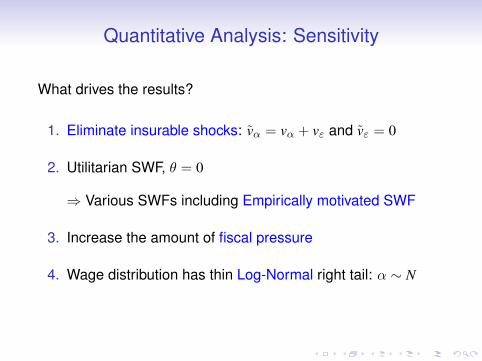
Sensitivity: Alternative SWFs

SWF Mirrlees Allocations Welfare Changeθ T ′(y) TR/Y ∆Y Mirrlees Affine HSV

Laissez-Faire −1 0.083 −0.082 9.72 3.15 3.14 2.98Emp. Motivated −0.57 0.314 0.051 0.16 0.05 −0.48 −

Utilitarian 0 0.491 0.213 −7.99 2.48 1.77 2.08Rawlsian ∞ 0.711 0.538 −22.55 708.28 649.14 354.90

Empirically-Motivated SWF

−2 −1 0 1 2−3

−2

−1

0

1

2

A. Log Consumption

α

MirrleesHSV

−2 −1 0 1 20.3

0.4

0.5

0.6

0.7

0.8

0.9

1B. Hours Worked

α

−2 −1 0 1 2−0.2

0

0.2

0.4

0.6

0.8C. Marginal Tax Rate

α−2 −1 0 1 2

−3

−2

−1

0

1D. Average Tax Rate

α

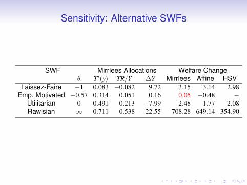
HSV vs Affine with Various SWFs

−1 −0.5 0 0.5

0

1

2

3

4

5

6

7W

elfa

re G

ains

(%

)

Taste for Redistribution (θ)−0.878 0.160

MirrleesHSVAffine

SWF Sensitivity: Summary

• Optimal tax system very sensitive to assumed SWF

• Welfare gains moving from the current tax system to the optimalone can be tiny

• Affine system works well when preference for redistribution iseither very strong or very weak:

• In the first case, want large lump-sum transfers

• In the second, want lump-sum taxes

• For intermediate tastes for redistribution (θ ∈ [−0.88, 0.16]),HSV is better than affine

Sensitivity: Stronger Fiscal Pressure

• Saez (2001) found a U-shaped marginal schedule to beoptimal

• His intuition: Want to make sure welfare is targeted only tothe very poor

• We don’t find this. Why?

• Key is degree of revenue requirement: to finance• exogenous public expenditure G• endogenous universal lump-sum transfers Tr

Increasing versus U-Shaped Marginal Rates

• Tax rates at the top always tend to be high• Extract as much tax revenue as possible (close to the top of

the Laffer curve)• Asymptotic rates indicated by Saez (2001): 1+σ

σ+λα

• Tax rates in the middle tend not to be high• Keep labor supply distortions low where the heaviest

population mass is located

• Tax rates at the bottom sensitive to fiscal pressure• Enough revenue from taxing the rich⇒ low rates⇒

increasing schedule• More fiscal pressure⇒ higher rates⇒ declining or

U-shaped schedule

U-shaped Tax Rates with High G

−2 −1 0 1 2−6

−4

−2

0

2

4A. Log Consumption

α

−2 −1 0 1 2

0.4

0.6

0.8

1

B. Hours Worked

α

−2 −1 0 1 20

0.2

0.4

0.6

0.8

1C. Marginal Tax Rate (with α)

α0 1 2 3 4 5 6

0

0.2

0.4

0.6

0.8

1D. Marginal Tax Rate (with income)

Income (y)

Baselineg = 0.50g = 0.75

Alternative Ways to Increase Fiscal Pressure

−2 −1 0 1 20

0.1

0.2

0.3

0.4

0.5

0.6

0.7

0.8

0.9

1A. Marginal Tax Rate (with α)

α

Baselineθ = 1No private insuranceElastic labor, σ = .5

0 1 2 3 4 5 60

0.1

0.2

0.3

0.4

0.5

0.6

0.7

0.8

0.9

1

Income (y)

B. Marginal Tax Rate (with income)

Reinterpreting the Literature

• Why does Saez (2001) find U-shaped rates?• Saez calibration implies very high fiscal pressure, in part

because he rules out private insurance

• U-shaped profile for marginal rates not a general feature ofan optimal tax system

• Diamond-Saez equation provides limited intuition for theshape of the optimal schedule

Sensitivity: Log-Normal Wage

Tax System Tax Parameters Outcomeswelfare Y T ′(y) TR/Y

HSVUS λ : 0.828 τ : 0.161 − − 0.319 0.017

HSV λ : 0.813 τ : 0.285 0.88 −5.20 0.427 0.048

Affine τ 0 : −0.230 τ 1 : 0.451 2.19 −6.01 0.451 0.242

Mirrlees 2.28 −5.74 0.443 0.254

• Log-normal distribution⇒ thin right tail

• Optimal HSV worse than optimal affine

• Optimal affine nearly efficient

Why Distribution Shape Matters

• Want high top marginal rates when (i) few agents facethose marginal rates, but (ii) can capture lots of revenuefrom higher-income households

0 2 4 6 80

0.2

0.4

0.6

0.8

1

Coeffi

cient

1−F(y

)y·f(y

)

Income (y)

Baseline: Pareto Log−NormalLog−Normal

0 2 4 6 80

0.1

0.2

0.3

0.4

0.5

0.6

0.7

Mar

gina

l Tax

Rat

e

Income (y)

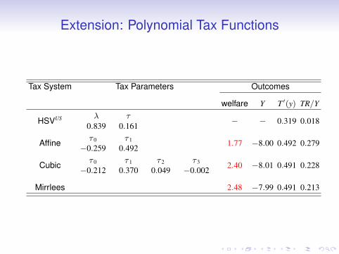
Extension: Polynomial Tax Functions

Tax System Tax Parameters Outcomes

welfare Y T ′(y) TR/Y

HSVUS λ0.839

τ0.161

− − 0.319 0.018

Affine τ 0

−0.259τ 1

0.4921.77 −8.00 0.492 0.279

Cubic τ 0

−0.212τ 1

0.370τ 2

0.049τ 3

−0.0022.40 −8.01 0.491 0.228

Mirrlees 2.48 −7.99 0.491 0.213

Cubic Tax Function

−2 −1 0 1 2−2

−1

0

1

2

A. Log Consumption

α

−2 −1 0 1 20.3

0.4

0.5

0.6

0.7

0.8

0.9

1B. Hours Worked

α

−2 −1 0 1 20

0.1

0.2

0.3

0.4

0.5

0.6

0.7

C. Marginal Tax Rate

α

−2 −1 0 1 2−8

−6

−4

−2

0

D. Average Tax Rate

α

MirrleesCubic

Extension: Type-Contingent Taxes

• Productivity partially reflects observable characteristics(e.g. education, age, gender)

• Some fraction of uninsurable shocks are observable:α→ α+ κ

• Heathcote, Perri & Violante (2010) estimate variance ofcross-sectional wage dispersion attributable toobservables, vκ = 0.108

• Planner should condition taxes on observables: T(y;κ)

• Consider two-point distribution for κ (college vs highschool)

Extension: Type-Contingent Taxes

• Significant welfare gains relative to non-contingent tax

• Conditioning on observables⇒ marginal tax rates of 42%

System Outcomeswel. Y T ′(y) TR/Y

HSVUS λ : 0.834,τ : 0.161 − − 0.3190.0150.020

HSVλL : 1.069, τL : 0.480

λH : 0.595, τH : 0.0736.21 −2.80 0.416

0.147−0.019

AffineτL

0 : −0.403, τL1 : 0.345

τH0 : −0.032, τH

1 : 0.4526.15 −2.53 0.421

0.4200.008

Mirrlees 6.54 −2.53 0.4180.3680.007

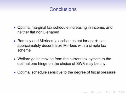
Conclusions

• Optimal marginal tax schedule increasing in income, andneither flat nor U-shaped

• Ramsey and Mirrlees tax schemes not far apart: canapproximately decentralize Mirrlees with a simple taxscheme

• Welfare gains moving from the current tax system to theoptimal one hinge on the choice of SWF, may be tiny

• Optimal schedule sensitive to the degree of fiscal pressure