1

Demand‐Side Factors in Optimal Land Conservation Choicea 

    

Amy W. Ando and Payal Shah  

Department of Agricultural and Consumer Economics University of Illinois at Urbana‐Champaign 

amyando@illinois.edu; psshah3@illinois.edu    

Selected Paper prepared for presentation at the Agricultural & Applied Economics Association 2009 AAEA & ACCI Joint Annual Meeting, Milwaukee, Wisconsin, July 26‐29, 2009 

  Copyright 2009 by Amy W. Ando and Payal Shah. All rights reserved. Readers may make verbatim copies of this document for non‐commercial purposes by any means, provided that this copyright notice appears on all such copies.         a This paper is based in part upon work supported by the Cooperative State Research, Education, and Extension Service, U.S. Department of Agriculture, under Project No. ILLU 05‐0305. We are grateful to Heidi J. Albers for extensive and inspiring conversations when this project was first being developed. We also received helpful comments from Ed Barbier and from participants in the Workshop on Spatial Environmental Economics at the University of Wyoming and the pERE Workshop at the University of Illinois. The authors retain responsibility for all errors within.    

2

I. Introduction 

The dominant current paradigm of conservation‐reserve planning in economics is to 

optimize the provision of physical conservation benefits (measured in units like acres or species 

protected) given a budget constraint. The basic idea conveyed by the academic literature to 

conservation planners and wildlife managers is that one should choose lands for nature 

reserves that are ecologically rich, not too expensive, and in threat of conversion away from 

natural state. Yet conservation planning in practice does not follow a cookie‐cutter approach. In 

fact, real analyses of optimal conservation site selection are done at widely divergent scales: 

intra‐state priority setting is embodied in state wildlife action plans (SWAPs);1 national‐level 

hot‐spot analysis concentrates conservation attention on a few places in Hawaii, California, the 

Appalachian Mountains, Florida, and the Great Basin (Stein et al., 2000); the World Wildlife 

Fund focuses its conservation activity at just 19 biodiversity hot‐spot areas in the world.  

This diversity of practice makes clear there are important outstanding questions in the 

science of site‐selection: what scale of conservation planning makes sense? Should we forget 

about implementing the Iowa SWAP and devote those resources to protecting the forests of 

the Amazon? Large‐scale biology‐based priority setting (such as that employed by WWF) 

implies that the value we place on biodiversity and ecosystem function is not affected by 

human proximity to that natural capital. There is significant evidence, however, that human 

willingness to pay (WTP) for conservation declines with distance (e.g. Loomis 2000) – a 

phenomenon we refer to as “spatial value decay”. How are optimal land conservation strategies 

affected by such localized preferences? Even at a given planning scale, how much should 

1 For information about SWAPs see http://www.wildlifeactionplans.org/.  

3

decision makers work to take account of the proximity of reserves to humans in the landscape? 

This paper begins a new strand of the reserve‐site selection literature that takes demand‐

side factors – the location of people in the landscape and the degree to which their preferences 

are localized – into account. We use theoretical simulations that are not tied to conditions in 

any one geographical location to explore the impact of demand‐side factors on two facets of 

optimal conservation choices: siting of a single reserve when conservation value is greatest 

near a critical site in the landscape (optimal targeting), and siting of multiple reserves when 

fragmentation reduces physical conservation services produced (optimal agglomeration). We 

also evaluate the increase in social well‐being that could be gained by using education 

campaigns to reduce individuals’ spatial decay factors while holding their maximum WTP for 

conservation constant. 

II.  Relevant literature 

Numerous papers find evidence of spatial value decay in household WTP for 

conservation.2 Hannon (1994) captures human preferences for nearness to objects they like 

and distances from objects they dislike. His results (using public opinion surveys) indicate that 

the spatial value decay function is one of exponential decline with respect to distance. In other 

papers, economists have used valuation methods to estimate relationships between WTP and 

distance of household to the thing that is being protected. Sutherland and Walsh (1985) use 

travel‐cost analyses of WTP for recreational amenities. They conclude that not only does WTP 

decrease with an increase in the distance, but it reaches zero beyond a given geographic 

2The spatial value decay in our model is functionally similar to iceberg transportation costs in new economic geography models (McCann 2005), though the two concepts have different motivational foundations, and our current work uses linear rather than exponential decay. 

4

distance. Pate and Loomis (1997) find that distance affects WTP a great deal for environmental 

programs with local, use‐value based importance, and much less for amenities with nationally‐

recognized non‐use value. Loomis (2000) estimates linear and log‐linear relationships between 

household WTP and distance from eight different environmental amenities, and finds 

significant negative effects of distance on WTP. The exact rate of spatial value decay ranges 

across amenities, but WTP falls by at least 50% after 2,000 miles.  

Work outside of the valuation literature also finds hints of spatial value decay. Albers et 

al. (2008) find that in Massachusetts, private conservation agents seem largely to protect 

township resources to an extent that varies with income and education levels in the town, 

rather than making tradeoffs across different parts of the state based on ecological richness. 

Nelson et al. (2007) and Kotchen and Powers (2006) document large support for local 

referendums that dedicate conservation resources in localized areas.  

Why does spatial value decay exist? At least three explanations emerge from literature. 

First, close proximity increases access to use values. This simple fact may explain why spatial 

value decay is less an issue with conservation targeted at amenities with large non‐use values. 

Second, Hannon (1994) claims that what he calls “geographic discounting” comes from people 

having a “sense of place” which is less localized, for example, in people who move around 

often. Third, Sutherland and Walsh (1985) emphasize that proximity increases the likelihood 

that a person will be well informed about the conservation services in question. The latter two 

sources of this phenomenon are not related to physical access, which raises the possibility that 

education and outreach could reduce spatial decay in human WTP for environmental amenities.  

This paper seeks to incorporate spatial value decay into the study of optimal reserve‐site 

5

selection. That literature has focused largely on optimizing production of physical conservation 

services. Early work by non‐economists pointed to prioritizing hot spots (Margules et al. 1988). 

The literature evolved to include other considerations such as variation in land costs (Ando et 

al. 1999) and degree of threat from development (Costello and Polasky 2004). The literature on 

optimal agglomeration has focused on tradeoffs between the harm of fragmentation to 

ecosystem functions and the danger of spatially correlated risks (Horan et al. 2008).  

Only a few studies of reserve design have deviated at all from the implicit assumption 

that the value of nature is invariant to its proximity to humans. Ruliffson et al. (2003) use 

integer programming to maximize species coverage and public “access” in the Chicago area, 

where access is defined as having reserves within a specified distance of towns. Onal and 

Yanprechaset (2007) do a similar analysis, maximizing the number of birds protected in Illinois 

subject to access and fragmentation constraints. This paper differs from that work in several 

important ways. First, it is difficult to derive general lessons integer‐programming analyses of a 

single real landscape because the results are strongly affected by the data (Ruliffson et al. 

(2003) mention this explicitly); we carry out stylized analyses of a wide variety of landscapes, 

which frees us from that limitation. Second, we study generalized spatial value decay rather 

than assuming an arbitrary requirement for urban access. This permits us to study the 

implications of such localized preferences when use‐value access is not an issue, evaluate the 

effects of a campaign to reduce the rate at which WTP declines with distance, and develop rules 

of thumb for how optimal “access” varies among conservation planning problems. 

III. Models 

We employ two models in order to highlight two different facets of optimal 

6

conservation planning. This approach also permits us to present the problem in two 

qualitatively different ways; the first is consistent with a welfare maximization problem 

common in neoclassical economics, while the other shows the importance of demand‐side 

factors in more practical terms that may resonate with agency conservation planners. This 

section provides an analytical description of the models. We then do numerical analyses 

(methodology described and results presented in the next two sections) to explore how 

characteristics of optimal reserve planning in the face of localized preferences depends on 

parameters of the situation. 

In both models we assume a linear abstract landscape (borrowing from the spirit of 

Hotelling’s linear city model) with variable width equal to k. A population of N people are 

distributed across the landscape with probability density f(x), where f(x) is a triangular 

distribution where e and f are the lower and upper limits of the range over which the density is 

non‐zero and g is the mode of the population distribution3. If we normalize the total population 

to equal one, the triangular distribution is: 

2( ) 2( )( | , , ) ( ); ( ); 0( )( ) ( )( )

x e f xf x e g f for e x g for g x f otherwisef e g e f e f g

− −= < < < <

− − − −   (1) 

One can interpret the scenarios with people distributed across a wide span of space as being 

relevant to planning problems in relatively rural or intensely urban areas where there is little 

spatial variation in the density of human settlement. Scenarios with a narrow triangular 

population distribution will provide insight into planning problems where there are large 

3 In results not reported in this paper, we also analyze scenarios in which the population follows different types of distribution. Given a population that is uniformly distributed in space, we obtain results that are very similar to scenarios with the triangular distribution and a wide population span. Results are somewhat different when we use a discrete bi‐modal population distribution; the distance between the two population modes strongly influences the optimal degree of fragmentation. Optimal policy pulls each site to be located near a different peak of the population distribution, which in effect increases the optimal degree of fragmentation.  

7

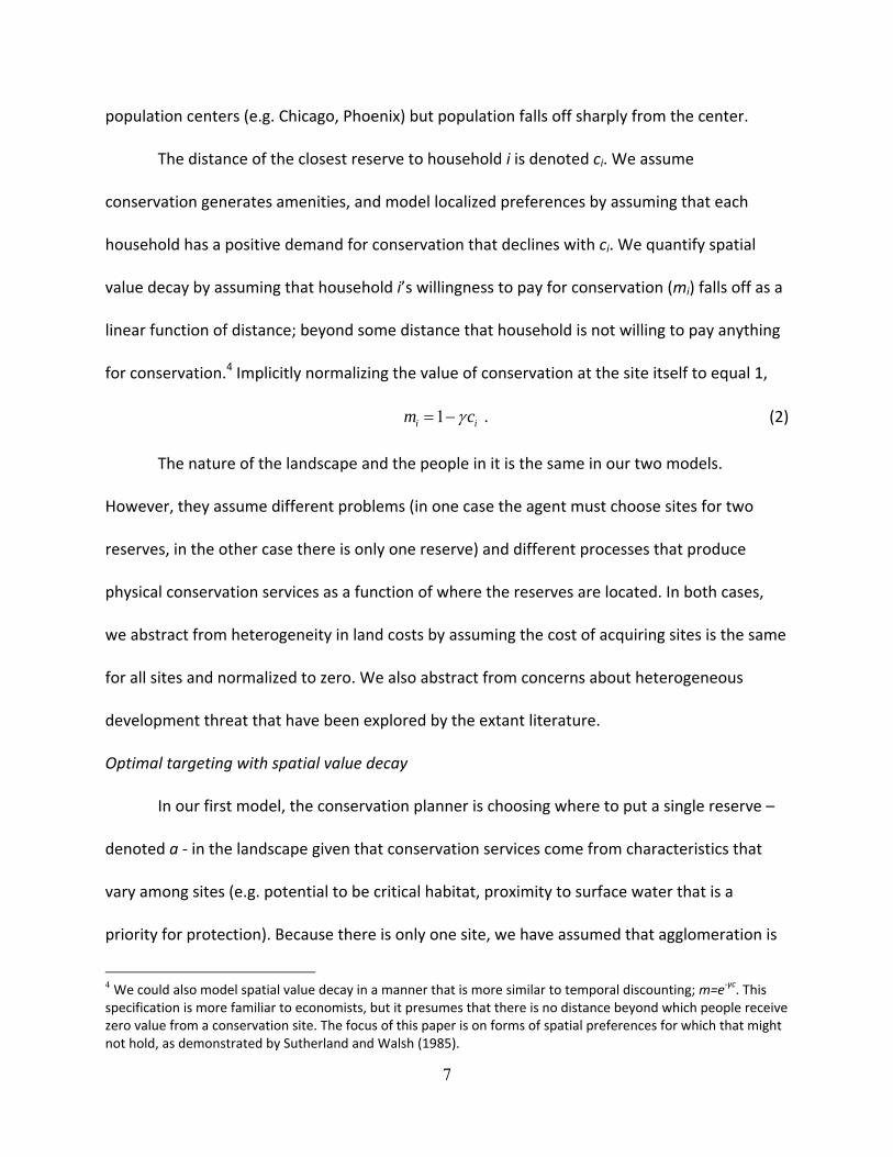
population centers (e.g. Chicago, Phoenix) but population falls off sharply from the center. 

The distance of the closest reserve to household i is denoted ci. We assume 

conservation generates amenities, and model localized preferences by assuming that each 

household has a positive demand for conservation that declines with ci. We quantify spatial 

value decay by assuming that household i’s willingness to pay for conservation (mi) falls off as a 

linear function of distance; beyond some distance that household is not willing to pay anything 

for conservation.4 Implicitly normalizing the value of conservation at the site itself to equal 1,  

1i im cγ= −  .            (2) 

The nature of the landscape and the people in it is the same in our two models. 

However, they assume different problems (in one case the agent must choose sites for two 

reserves, in the other case there is only one reserve) and different processes that produce 

physical conservation services as a function of where the reserves are located. In both cases, 

we abstract from heterogeneity in land costs by assuming the cost of acquiring sites is the same 

for all sites and normalized to zero. We also abstract from concerns about heterogeneous 

development threat that have been explored by the extant literature. 

Optimal targeting with spatial value decay 

In our first model, the conservation planner is choosing where to put a single reserve – 

denoted a ‐ in the landscape given that conservation services come from characteristics that 

vary among sites (e.g. potential to be critical habitat, proximity to surface water that is a 

priority for protection). Because there is only one site, we have assumed that agglomeration is 

4 We could also model spatial value decay in a manner that is more similar to temporal discounting; m=e‐γc. This specification is more familiar to economists, but it presumes that there is no distance beyond which people receive zero value from a conservation site. The focus of this paper is on forms of spatial preferences for which that might not hold, as demonstrated by Sutherland and Walsh (1985). 

8

not a factor in the problem. However, we assume conservation services fall off from one critical 

location A (which varies in the landscape randomly in different draws of the problem).  

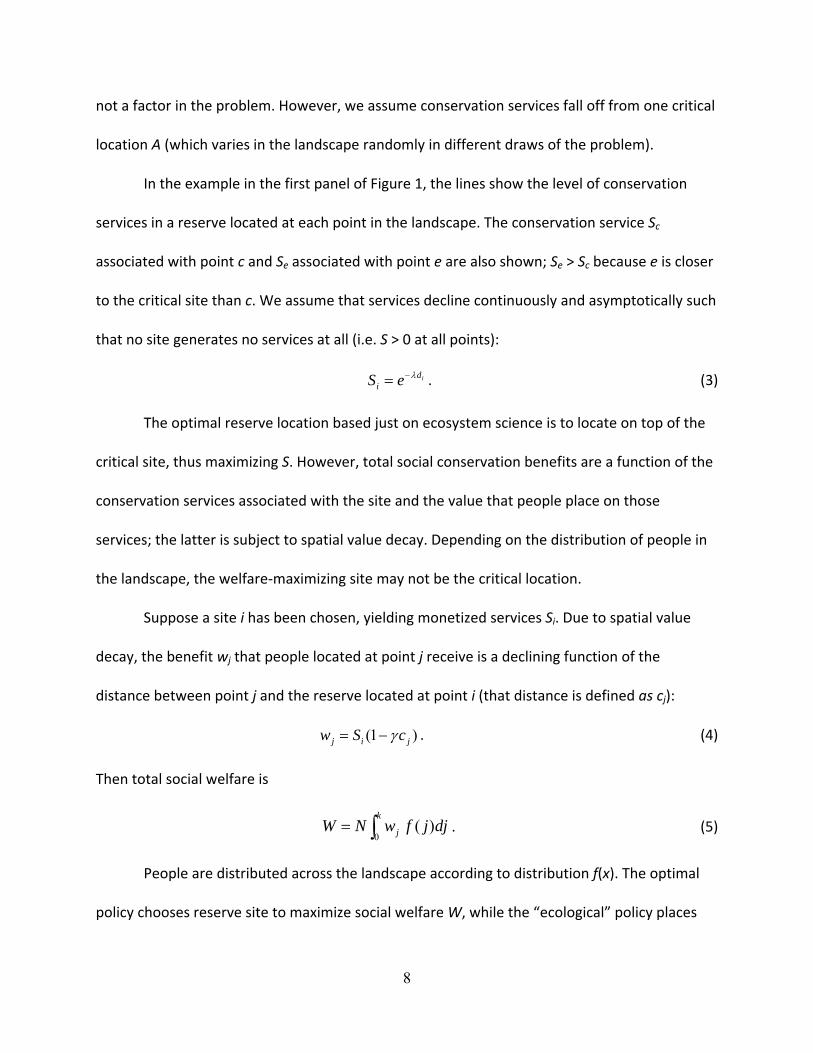
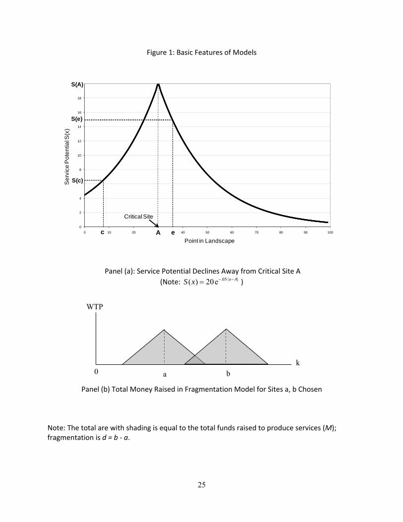
In the example in the first panel of Figure 1, the lines show the level of conservation 

services in a reserve located at each point in the landscape. The conservation service Sc 

associated with point c and Se associated with point e are also shown; Se > Sc because e is closer 

to the critical site than c. We assume that services decline continuously and asymptotically such 

that no site generates no services at all (i.e. S > 0 at all points): 

idiS e λ−= .            (3) 

The optimal reserve location based just on ecosystem science is to locate on top of the 

critical site, thus maximizing S. However, total social conservation benefits are a function of the 

conservation services associated with the site and the value that people place on those 

services; the latter is subject to spatial value decay. Depending on the distribution of people in 

the landscape, the welfare‐maximizing site may not be the critical location. 

Suppose a site i has been chosen, yielding monetized services Si. Due to spatial value 

decay, the benefit wj that people located at point j receive is a declining function of the 

distance between point j and the reserve located at point i (that distance is defined as cj): 

(1 )j i jw S cγ= − .            (4) 

Then total social welfare is 

 0

( )k

jW N w f j dj= ∫ .            (5) 

People are distributed across the landscape according to distribution f(x). The optimal 

policy chooses reserve site to maximize social welfare W, while the “ecological” policy places 

9

the reserve on the critical site. We carry out simulations in which features of the population 

distribution, the location of the critical site, the rapidity with which services decline with 

distance to the critical site, and the extent of spatial value decay are all allowed to vary.  

Optimal agglomeration with spatial conservation value decay 

This model differs from the first model in two ways. First, it assumes there are no critical 

sites but agglomeration is an important feature of a network of reserves. Second, it deviates 

from a neo‐classical economics model of welfare maximization in that the conservation agent is 

maximizing physical quantities of conservation services (e.g. species populations, effectiveness 

of flood control) rather than maximizing social welfare.  

  The conservation agent is choosing where to locate two sites, a and b; let d denote the 

distance between those sites: d b a= − . All points in the landscape have the same 

conservation potential, but conservation services are diminished by fragmentation d. Once the 

agency chooses the site locations, it tries to raise money to support activities (such as active 

stewardship at the sites) that increase the conservation services that emerge from the sites.  

The amount of money a person is willing to give to support the sites is subject to spatial 

value decay. In particular, we assume that citizen willingness to support a conservation reserve 

is not affected by the degree of fragmentation, so a person at point i donates money mi exactly 

according to equation (2). We are also implicitly assuming that citizens have strong downward 

sloping demand for natural amenities, and their value is affected only by the proximity of the 

closest reserve and not by the presence of other reserves in the network.5 

The total amount of money collected by the agency is   5 This assumption is strong, but consistent with evidence of downward‐sloping demand for endangered species listings in a given area (Ando 2001). Future work could model this element of consumer welfare in more detail.  

10

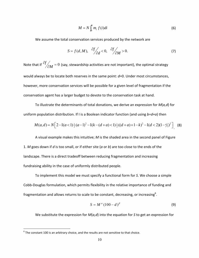
0( )

k

iM N m f i di= ∫             (6) 

We assume the total conservation services produced by the network are 

  ( , ), 0, 0.f fS f d M d M∂ ∂= < >∂ ∂         (7) 

Note that if  0=∂∂

Mf  (say, stewardship activities are not important), the optimal strategy 

would always be to locate both reserves in the same point: d=0. Under most circumstances, 

however, more conservation services will be possible for a given level of fragmentation if the 

conservation agent has a larger budget to devote to the conservation task at hand. 

To illustrate the determinants of total donations, we derive an expression for M(a,d) for 

uniform population distribution. If I is a Boolean indicator function (and using b=d+a) then 

2 2 21 122 2( , ) 2 ( 1) ( 1) ( ( ) 1) (( ) 1 ) ( 2)(1 )dM a d N a a k d a d a k d⎡ ⎤= −Ι < − −Ι − + < + + − −Ι < −⎣ ⎦ .

   (8) 

A visual example makes this intuitive; M is the shaded area in the second panel of Figure 

1. M goes down if d is too small, or if either site (a or b) are too close to the ends of the 

landscape. There is a direct tradeoff between reducing fragmentation and increasing 

fundraising ability in the case of uniformly distributed people. 

To implement this model we must specify a functional form for S. We choose a simple 

Cobb‐Douglas formulation, which permits flexibility in the relative importance of funding and 

fragmentation and allows returns to scale to be constant, decreasing, or increasing6. 

(100 )S M dα β= −           (9) 

We substitute the expression for M(a,d) into the equation for S to get an expression for 

6 The constant 100 is an arbitrary choice, and the results are not sensitive to that choice. 

11

S(a,d). The optimal reserve design maximizes conservation services S by choosing a location a 

and degree of fragmentation d that strikes the best balance between fragmentation and local 

appeal. The ecological policy minimizes fragmentation. When population is uniformly 

distributed, the location parameter a is chosen randomly, while when population has a 

triangular distribution, both reserves are placed on the mode of the population distribution so 

as not to penalize the ecological policy unnecessarily. We carry out simulations in which 

features of the population distribution, the parameters of the Cobb‐Douglas conservation 

service production function, and the rate of spatial value decay are all allowed to vary.  

IV. Simulation methods 

We carry out two types of simulations to gain insight into the nature of optimal 

conservation policy when a decision maker takes into account demand‐side factors. We seek to 

understand the differences between optimal policies and policies informed only by ecological 

concerns, both in terms of the choices made and the benefits that result from those choices. 

The current simulations assume N = 10,000, but qualitative results are not sensitive to 

that choice. The first sets of simulations use Monte Carlo simulations of the fragmentation and 

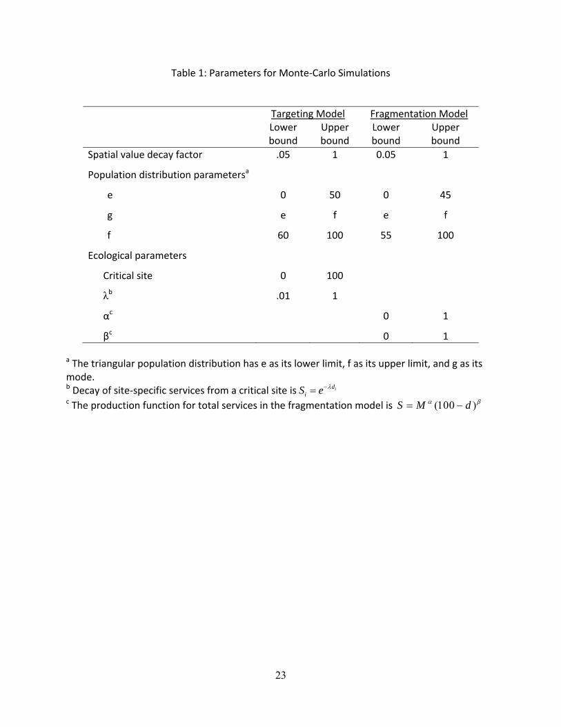
targeting models described above. We conduct 1,000 runs for each model. A single run takes a 

set of parameters that are randomly chosen from uniform distributions parameterized as in 

Table 1; that set of parameters serves to describe the population distribution, spatial value 

decay, and ecological production function. For those parameters, the ecological policy decision 

is determined, and the optimal policy is found using a simplex grid search method. The social 

welfare or level of total services is determined for each of those policies. The results are 

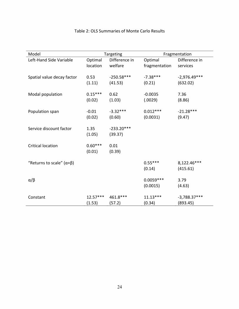
summarized using OLS regressions that are reported in Table 2. The data in the regressions are 

12

features of deterministic simulations, and thus the regression results cannot be interpreted in 

the usual way. However, OLS regressions provide a compact vehicle for summarizing how 

important outcomes are affected by the parameters of the scenario. 

We also carry out simulations for each model that vary only two parameters at a time 

while holding others constant. With this work we generate figures that illustrate clearly how 

outcomes (fragmentation, site‐selection location, difference in welfare or total services caused 

by using optimal policy) change with variation in a few key parameters (Figures 2‐ 9.) These 

figures reveal effects that are non‐linear or dependent on interactions between parameters. 

V. Results 

A. Targeting Model 

  Our first results help us understand how optimal site‐selection decisions in a targeting 

framework might deviate from the ecological priority site. The first column of Table 2 presents 

OLS results that summarize factors that influence the optimal location for the site. The optimal 

location is pulled toward the critical site and toward the center of population density. The other 

factors – service discount factor, spatial value decay factor, and population span – play more 

complicated roles in this problem that do not yield significant coefficients in a linear regression. 

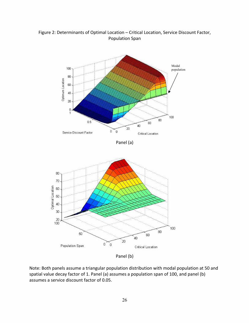
  We can better understand the tension between the critical site and the site of heaviest 

population density by looking at panel (a) of Figure 2. If the service discount factor is very low, 

meaning the critical site is not really very critical, the optimal site is near the mode of the 

population distribution. However, the optimal site hews closely to the ecological critical site for 

13

all service discount factors above 0.1.7  

The second panel of Figure 2 makes clear that the pull of a population center depends 

on how widely scattered people are around it. For wider population spans (where the 

population mode is at the center), the optimal conservation site moves with the critical 

location. However, if people are tightly clustered, the optimal location remains close to the 

mode of the population distribution even if the critical location is far away. Indeed, not until the 

population span is a fourth of the total landscape size does the optimal site location begin to 

move toward the critical site with increasing population span. When spatial value decay is 

present and people are tightly concentrated in the landscape, no social value will be gained 

from protecting a site that is far away from people no matter how ecologically valuable it is.   

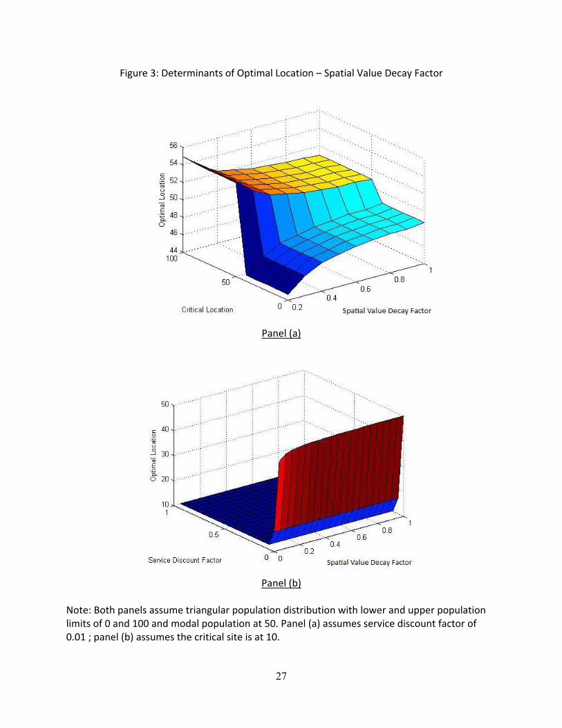
Under some circumstances, the relative intensity of spatial value decay has a modest 

impact on the optimal site‐selection choice. The first panel of Figure 3 shows that if services do 

not fall off rapidly from the ecologically‐critical site (λ=.01), the optimal site is closer to the 

population center when spatial value decay is strong. If one can shift the chosen site away from 

the critical site without sacrificing too much benefit potential, the payoff to moving the site 

toward people is larger when those people have localized preferences. The second panel 

confirms that if the service discount factor is extremely low so the landscape is fairly 

homogeneous in ecological value, the optimal location moves closer to the population center as 

the spatial value decay factor increases from very low to intermediate values. However, all 

those optimal locations are fairly close to the population mode, and the optimal site does not 

vary with the spatial value decay factor over a wide range of service discount factors. 

7 To put that in perspective, if the landscape is 390 miles long (like the state of Illinois), λ=0.1 implies that service potential falls by half within 27 miles of the critical site. 

14

The rate of spatial value decay does, however, have a large impact on the extent to 

which a change from ecological policy to optimal policy can increase social welfare. Table 2 

shows that increasing the spatial value decay factor, the span of the population distribution, 

and the service discount factor decreases the absolute change in welfare that results from 

making the optimal instead of ecological policy choice.  

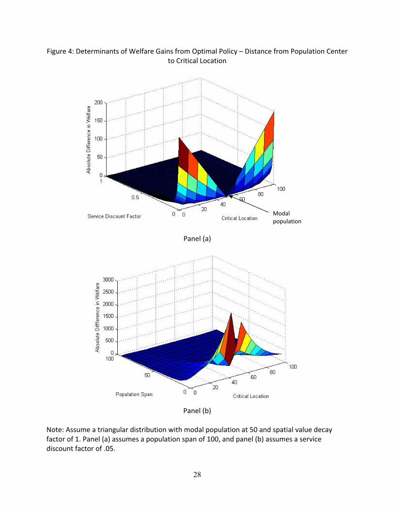
Figure 4 demonstrates some key factors in determining whether much can be gained by 

using the optimal policy. It is most important for planners to use optimal instead of ecological 

policy when the critical location is not too critical and the critical location is not near the modal 

population. The first factor matters because if the service discount factor is small, there will not 

be a large penalty for making a choice that pulls the protected site away from the critical site 

that would have been chosen by the ecological policy. The percentage change in welfare can 

still be as large as 100% when the service discount factor is large and the critical location is at 

some distance from the modal population, but only because welfare is low under both policies. 

The second factor plays a big role because if the critical location happens to be right on top of 

the mode of the population distribution, then the “optimal” policy would not recommend 

anything much different from the ecological policy, and welfare is high in both scenarios.  

However, if the critical location is very far away from the population center, then even optimal 

policy will have trouble yielding large levels of welfare.  

We see from the second panel of Figure 4 that optimal policy can also yield large 

increases in welfare when the critical location is at a moderate distance from the population 

center if the population span is very tight. Given the opposite – broad dispersion of people 

throughout the landscape – a fair number of people will gain value from a protected site that is 

15

placed on an ecological hot spot even if that spot is far from the place that happens to have the 

largest number of people. Thus, the optimal policy does little to correct a problem with 

ecological policy when people are not highly concentrated in space.  

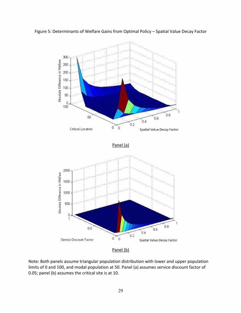
The spatial value decay factor has a strong effect on the importance of using optimal 

(rather than ecological) policy, as can be seen from Figure 5. If the critical location is not too 

critical and/or the critical site is not near the population center, there can be particularly large 

gains to using optimal strategy if preferences are non‐localized. In both panels of Figure 5 we 

see that the absolute gains from optimal policy are low when preferences are highly localized. 

However, the percentage gain in welfare is not affected by the extent of spatial value decay and 

can be as high as 70%, provided the critical location is not too critical. The problem is that 

localized preferences cause welfare to be relatively low under both policy scenarios, so the 

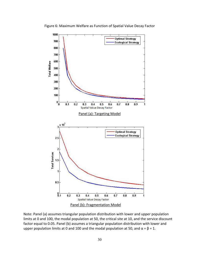
absolute magnitude of the difference between them is not large.  This effect is illustrated in the 

first panel of Figure 6, where spatial value decay must be very limited in order for welfare to 

rise above minimum levels. When travel costs or a strong “sense of place” cause people to have 

high spatial value decay factors, it is very difficult for a planner to choose a good site in the 

absence of serendipitous proximity between the ecologically critical site and where people live. 

B. Fragmentation Model 

The Monte‐Carlo results summarized in the third column of Table 2 indicates that 

several factors have significant and consistent effects on the optimal degree of fragmentation. 

When people have non‐localized preferences and when money is an important input (because 

stewardship matters or returns are increasing), optimal fragmentation is higher. Optimal 

fragmentation is also higher when people are widely dispersed in the landscape. 

16

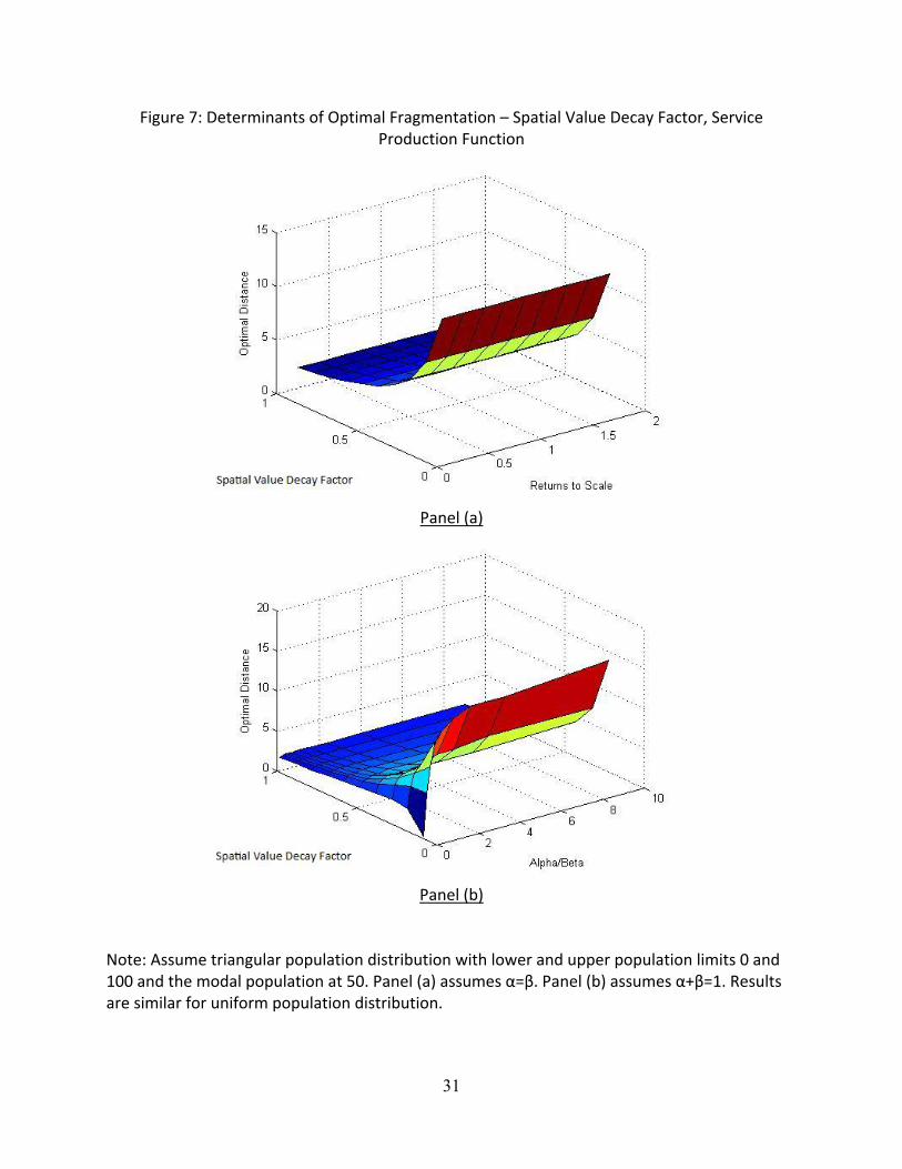
Some of these results are illustrated in Figure 7. In both panels, optimal fragmentation is 

smaller (and closer to the choice made under the ecological policy) for localized preferences. 

The intuition here is that if the spatial value decay factor is high, the degree of fragmentation 

beyond which more fragmentation fails to raise more money is relatively small. Given that 

fragmentation itself retards the production of conservation services, it is never optimal to 

choose a large distance between sites if it does not contribute to monetary inputs. We also see 

that when γ is low enough for fragmentation to help with fundraising, more fragmentation is 

optimal if (but only if) monetary inputs are important relative to agglomeration. When we run 

the fragmentation model with population scattered according to the triangular distribution, we 

also see that optimal fragmentation is higher when the span across which people are located is 

broader8. If people are not concentrated in a small area of the landscape, fragmentation can be 

an effective way to increase the funds available to manage the network of protected lands. 

The fourth column in Table 2 gives clues to the situations in which service provision is 

increased most by using optimal rather than straight ecological policy. The absolute difference 

in services is higher when preferences are non‐localized, when there are increasing returns to 

scale in service production, and when people are concentrated in the landscape.  

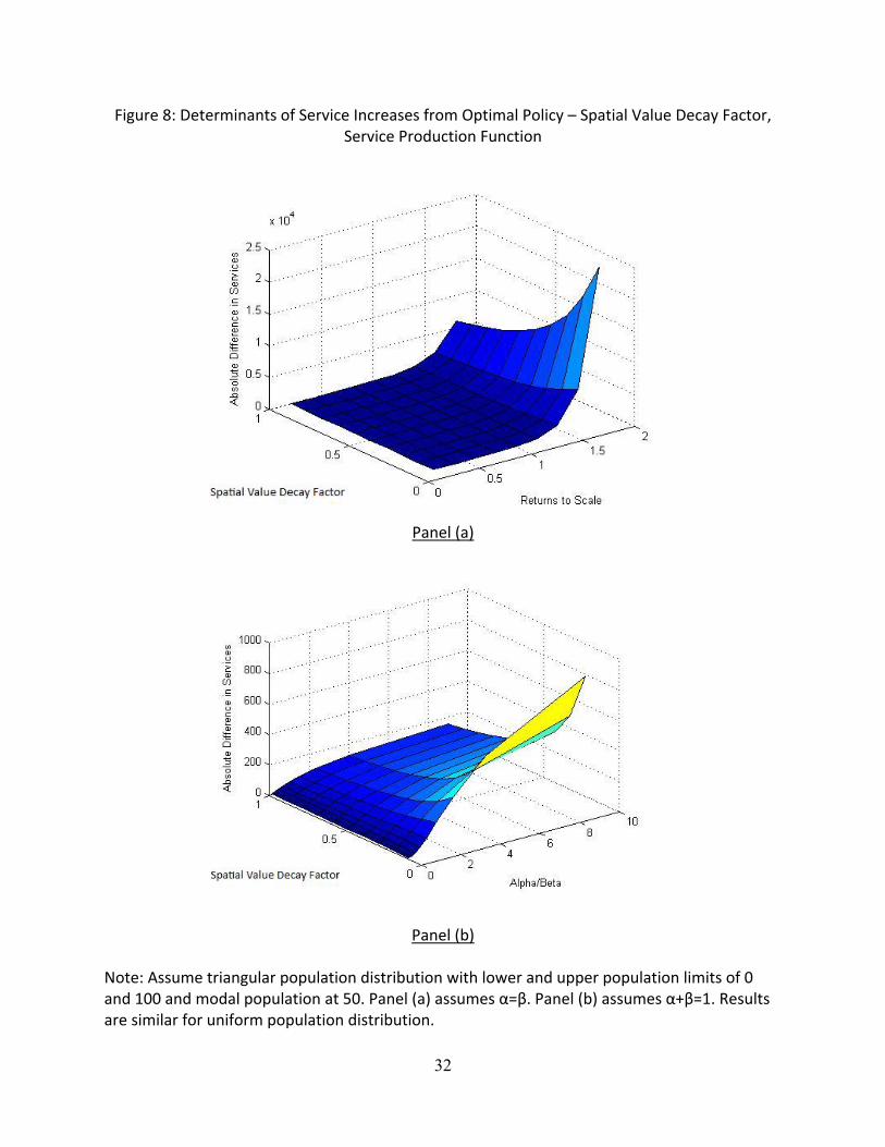
Figure 8 illustrates some of those effects. The absolute difference in services is small for 

a high spatial value decay factor; the maximum supply of money that can be raised is small 

when preferences are localized, so optimal policy cannot do much to increase services by 

deviating from the zero‐fragmentation arrangement. However, optimal policy is beneficial 

when we have increasing returns to scale and a large α/β, even if preferences are somewhat 

8 The figure is not shown in the current version of this paper. 

17

localized. The biggest payoff to society of using optimal policy is when preferences are not 

localized and fund‐raising provides inputs that are really important to service production. 

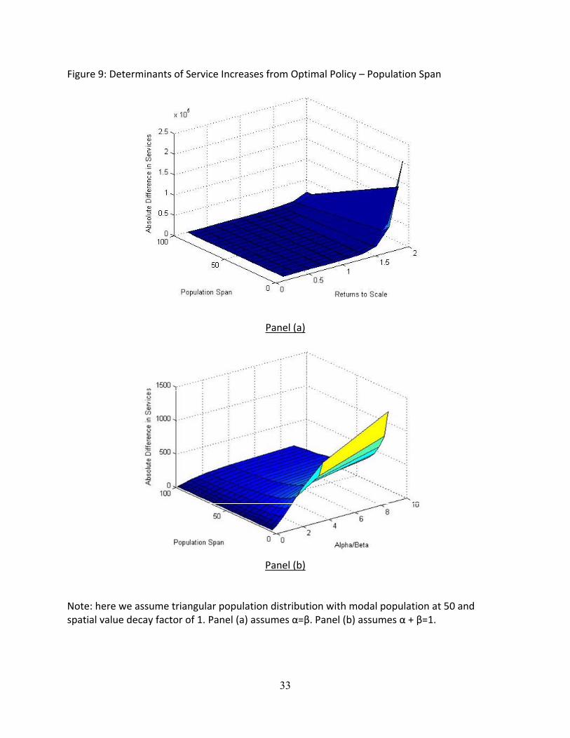
Figure 9 shows how optimal fragmentation varies with the dispersion of people. If 

people are spatially clustered, the absolute difference in services between policy regimes is 

large if fundraising is important to service provision (e.g. increasing returns to scale or high 

α/β.) With that population distribution it is easier to capture value from everyone, which 

increases the potential services that can be achieved with optimal policy when money matters. 

However, the percentage change in welfare is affected little by the distribution of people in 

space and can be as high as 50% for higher returns to scale. 

The second panel of Figure 6 shows that optimal policy increases services over an 

ecological policy of minimum fragmentation, even when the spatial value decay factor is high. 

Recall that our ecological policy does place the agglomerated network on the mode of the 

population distribution, so it is not assumed to be completely unresponsive to demand‐side 

factors. The gain in services shows what can be accomplished just by deviating from an ecology‐

based minimum fragmentation prescription.9 Note that both policies generate more services 

when the spatial decay factor is low. Efforts to increase citizens’ WTP for conservation outside 

their back yards might yield greater environmental services from either planning strategy. 

VI Conclusions 

This paper has launched a useful new strand of the conservation reserve design literature 

which takes into account “demand‐side” factors: the distribution of people in the landscape, 

9 Gains from optimal policy are higher if the ecological policy does not pay attention to the location of people and the minimally‐fragmented network is located with equal probabilities at any of the points in the landscape. Services from ecological policy are almost cut in half when the minimally‐fragmented network is located randomly in the landscape (e.g. at any of 1000 discrete points with equal probability). 

18

and the manner in which their willingness to pay for an environmental amenity depends on 

how far away that amenity is. We note that the exact analysis in this paper is only relevant for 

conservation that yields certain types of amenities. First, our spatial value decay function is 

applicable for conservation that yields environmental amenities near the conservation site 

itself. Prairie pothole conservation, for example, yields increases in waterfowl populations 

across a very wide geographic area, and thus would not usefully informed by this specific 

analysis. Second, the analysis in this paper presumes that people near a protected site gain 

benefits from the conservation activity. However, some kinds of wildlife actually cause serious 

problems for people living in close proximity to them. Society as a whole may value protection 

of such species, but there is a significant disamenity value for African farmers living very close 

to elephants, or Montana ranchers living close to wolves. Demand‐side factors should still be 

considered in developing such conservation plans, but the function that maps proximity into 

value would need to be more complex than the model we employ here. 

Our results make clear that when conservation does provide localized amenity values, 

sometimes planners should deviate from protecting places of highest ecological priority to 

move reserves near population centers with a high willingness to pay for conservation. 

However, we show it is not correct to assume that all towns should have “access” to reserves – 

it is not always optimal to deviate from the ecologically‐optimal level of fragmentation to 

increase proximity to broad range of people. Optimal access to reserves is case specific, and 

varies with ecological and socio‐economic features of the conservation problem at hand. 

How might optimal conservation planning differ from straight ecological prescriptions? 

While minimum fragmentation is often optimal, planners can usefully employ increased 

19

fragmentation to capture value when people’s preferences are not very highly localized. In a 

targeting problem, the ecologically critical site is often the right thing to protect, even when 

using a policy tool that worries about demand‐side factors. However, optimal policy balances 

proximity to critical site with proximity to people. The optimal reserve choice can move far 

away from the site of greatest ecological importance if the ecological “quality” of sites does not 

decline too much with distance from the ecological priority, and if human population is spatially 

concentrated such that value is not captured without moving the protected site near people. 

Conservation planners and managers will find it time‐consuming and resource intensive to 

invest in a decision making process that is more complex. It will not always be worth the added 

agency costs to do more than ecology‐based planning. Our results identify a few types of 

scenarios in which the payoff to using an optimal policy that considers demand‐side factors is 

large. Regardless of the particular planning problem at hand, it is most important to worry 

about demand‐side concerns if people are not evenly spread in the landscape, as in the case of 

a city surrounded by a rural area. 

The focus of some conservation planning problems is to locate a site in a landscape with 

heterogeneous ecological value. In such cases, the payoff to using optimal policy is large if the 

critical location is not too much higher in ecological value than other nearby sites in the 

surrounding landscape, and if the center of human population is a moderate distance away. 

Then, welfare can be much larger if the site is shifted away somewhat from the hot spot to 

increase the value people gain from the resources that are protected.  

The focus of the planning problem might instead be to decide how much fragmentation 

to allow in a network of reserves in which ecological services are not otherwise a function of 

20

location. For example, part of the Illinois SWAP calls for development of a network of restored 

grasslands; agglomeration is desirable in that project, but there is huge area of farmland that is 

all equally suitable for restoration. In such a problem, there is a large payoff to considering 

demand‐side factors and choosing seemingly excessive levels of fragmentation if fundraising 

provides resources for stewardship activities (like mowing and controlled burns) that are 

valuable for increasing service flows from the network of reserves. Optimal policy is also 

particularly helpful in the fragmentation problem if people’s preferences are not too localized, 

such that there is a larger pool of willingness to pay for conservation to be captured. 

In general, we find that spatial value decay reduces the maximum levels of welfare and 

environmental services that can be gained from any conservation‐planning approach. When 

spatial value decay is present because people are simply unaware of environmental resources 

farther away from where they live, education campaigns might serve to increase social welfare 

and environmental services. However, more research is needed to evaluate whether it possible 

for such campaigns to reduce spatial value decay enough to make a difference. 

Our models abstract from issues of heterogeneous land costs and development threats 

which have been well‐explored in the literature to date. In that previous work (e.g. Costello and 

Polasky 2004), a clear tension was present in deciding whether to locate conservation reserves 

near people; proximity to people drives up acquisition costs, but it also drives up the threat of 

imminent conversion and thus increases the social value of protecting the land. Our work 

introduces a third aspect of proximity to humans that may shift the balance in conservation 

planning towards favoring sites close to human population centers when conservation 

generates local natural amenities.  

21

References  

Albers, Heidi J., Amy W. Ando, and Xiaoxuan Chen. 2008. “A spatial‐econometric analysis of 

attraction and repulsion of private conservation by public reserves.” Journal of 

Environmental Economics and Management 56: 33‐49. 

Ando, Amy, Jeffrey Camm, Stephen Polasky, and Andrew Solow. 1998. “Species distributions, 

land values, and efficient conservation.” Science 279: 2126‐2128. 

Ando, Amy. 2001. “Economies of scope in endangered‐species protection: Evidence from 

interest‐group behavior.” Journal of Environmental Economics and Management 4(3): 

312‐332. 

Costello, Christopher and Stephen Polasky. 2004. “Dynamic reserve site selection.” Resource 

and Energy Economics 26(2): 157‐174 

Hannon, Bruce. 1994. “Sense of place: geographic discounting by people, animals and plants.” 

Ecological Economics 10(2): 157‐174. 

Horan, Richard D., Jason F. Shogren, and Benjamin M. Gramig. 2008. “Wildlife conservation 

payments to address habitat fragmentation and disease risks.” Environment and 

Development Economics 13: 415‐439.  

Kotchen, Matthew J. and Shawn M. Powers. 2006. “Explaining the appearance and success of 

voter referenda for open‐space conservation.” Journal of Environmental Economics and 

Management 52(1): 373‐390. 

Loomis, John B. 2000. “Vertically summing public good demand curves: An empirical 

comparison of economic versus political jurisdictions.” Land Economics 76(2): 312‐321. 

22

Margules, C. R., A. O. Nicholls, and R. L. Pressey. 1988. “Selecting networks of reserves to 

maximize biological diversity.” Biological Conservation 43(1): 4363‐76. 

McCann, Philip. 2005. “Transport costs and new economic geography.” Journal of Economic 

Geography 5(3): 305‐318. 

Nelson, Erik, Michinori Uwasu, and Stephen Polasky. 2007. “Voting on open space: What 

explains the appearance and support of municipal‐level open space conservation 

referenda in the United States?” Ecological Economics 62(3‐4): 580‐93. 

Önal, Hayri and Pornchanok Yanprechaset. 2007. “Site accessibility and prioritization of nature 

reserves.” Ecological Economics 60(4): 763‐773. 

Pate, Jennifer and John B. Loomis. 1997. “The effect of distance on willingness to pay values: a 

case study of wetlands and salmon in California.” Ecological Economics 20(3): 199‐207. 

Ruliffson, Jane A., Robert G. Haight, Paul H. Gobster, and Frances R. Homans. 2003. 

“Metropolitan natural area protection to maximize public access and species 

representation.” Environmental Science & Policy 6(3): 291‐299. 

Sutherland, Ronald J. and Richard G. Walsh. 1985. “Effect of distance on the preservation value 

of water quality.” Land Economics 61(3): 281‐291. 

Stein, Bruce A., Lynn S. Kutner, and Jonathan S. Adams. 2000. Precious heritage: The Status of 

biodiversity in the United States. Oxford University Press: New York. 

23

idiS e λ−=

Table 1: Parameters for Monte‐Carlo Simulations 

   Targeting Model  Fragmentation Model  Lower 

bound Upper bound 

Lower bound 

Upper bound 

Spatial value decay factor  .05  1  0.05  1 

Population distribution parametersa         

e  0  50  0  45 

g  e  f  e  f 

f  60  100  55  100 

Ecological parameters         

Critical site  0  100     

λb  .01  1     

αc      0  1 

βc      0  1  a The triangular population distribution has e as its lower limit, f as its upper limit, and g as its mode. b Decay of site‐specific services from a critical site is  c The production function for total services in the fragmentation model is  (100 )S M dα β= −  

24

Table 2: OLS Summaries of Monte Carlo Results     Model  Targeting  Fragmentation Left‐Hand Side Variable  Optimal 

location Difference in welfare 

Optimal fragmentation 

Difference in services  

Spatial value decay factor  0.53 (1.11) 

‐250.58*** (41.53) 

‐7.38*** (0.21) 

‐2,976.49*** (632.02)  

Modal population  0.15*** (0.02) 

0.62 (1.03)  

‐0.0035 (.0029) 

7.36 (8.86) 

Population span  ‐0.01 (0.02) 

‐3.32*** (0.60)  

0.012*** (0.0031) 

‐21.28*** (9.47)  

Service discount factor  1.35 (1.05) 

‐233.20*** (39.37)  

   

Critical location  0.60*** (0.01) 

0.01 (0.39)  

   

“Returns to scale” (α+β)      0.55*** (0.14) 

8,122.46*** (415.61)  

α/β      0.0059*** (0.0015) 

3.79 (4.63)  

Constant  12.57*** (1.53) 

461.8*** (57.2) 

11.13*** (0.34) 

‐3,788.37*** (893.45) 

    

25

Figure 1: Basic Features of Models  

  

 Panel (a): Service Potential Declines Away from Critical Site A (Note:  .05 | |( ) 20e x AS x − ⋅ −=  ) 

Panel (b) Total Money Raised in Fragmentation Model for Sites a, b Chosen 

   Note: The total are with shading is equal to the total funds raised to produce services (M); fragmentation is d = b ‐ a. 

0

2

4

6

8

10

12

14

16

18

20

0 10 20 30 40 50 60 70 80 90 100

Ser

vice

Pot

entia

l S(x

)

Point in Landscape

S(c)

S(e)

c e

Critical Site

A

S(A)

0 k

a b

WTP

26

Figure 2: Determinants of Optimal Location – Critical Location, Service Discount Factor, Population Span 

 

 Panel (a) 

 Panel (b) 

 Note: Both panels assume a triangular population distribution with modal population at 50 and spatial value decay factor of 1. Panel (a) assumes a population span of 100, and panel (b) assumes a service discount factor of 0.05.    

Modal population

27

Figure 3: Determinants of Optimal Location – Spatial Value Decay Factor  

 Panel (a) 

 

 Panel (b) 

 Note: Both panels assume triangular population distribution with lower and upper population limits of 0 and 100 and modal population at 50. Panel (a) assumes service discount factor of 0.01 ; panel (b) assumes the critical site is at 10. 

28

Figure 4: Determinants of Welfare Gains from Optimal Policy – Distance from Population Center to Critical Location 

 Panel (a) 

 Panel (b) 

 Note: Assume a triangular distribution with modal population at 50 and spatial value decay factor of 1. Panel (a) assumes a population span of 100, and panel (b) assumes a service discount factor of .05. 

Modal population 

29

Figure 5: Determinants of Welfare Gains from Optimal Policy – Spatial Value Decay Factor 

  

Panel (a) 

 Panel (b) 

 Note: Both panels assume triangular population distribution with lower and upper population limits of 0 and 100, and modal population at 50. Panel (a) assumes service discount factor of 0.05; panel (b) assumes the critical site is at 10. 

30

Figure 6: Maximum Welfare as Function of Spatial Value Decay Factor 

Panel (a): Targeting Model 

 

 Panel (b): Fragmentation Model 

Note: Panel (a) assumes triangular population distribution with lower and upper population limits at 0 and 100, the modal population at 50, the critical site at 10, and the service discount factor equal to 0.05. Panel (b) assumes a triangular population distribution with lower and upper population limits at 0 and 100 and the modal population at 50, and α = β = 1. 

31

Figure 7: Determinants of Optimal Fragmentation – Spatial Value Decay Factor, Service Production Function 

Panel (a) 

 Panel (b) 

  Note: Assume triangular population distribution with lower and upper population limits 0 and 100 and the modal population at 50. Panel (a) assumes α=β. Panel (b) assumes α+β=1. Results are similar for uniform population distribution.     

32

Figure 8: Determinants of Service Increases from Optimal Policy – Spatial Value Decay Factor, Service Production Function 

 

Panel (a) 

 

  

Panel (b)  Note: Assume triangular population distribution with lower and upper population limits of 0 and 100 and modal population at 50. Panel (a) assumes α=β. Panel (b) assumes α+β=1. Results are similar for uniform population distribution. 

33

Figure 9: Determinants of Service Increases from Optimal Policy – Population Span 

Panel (a) 

 Panel (b) 

  Note: here we assume triangular population distribution with modal population at 50 and spatial value decay factor of 1. Panel (a) assumes α=β. Panel (b) assumes α + β=1.