Optimal Location of Booster Chlorination Stations

7/27/2019 Optimal Location of Booster Chlorination Stations

http://slidepdf.com/reader/full/optimal-location-of-booster-chlorination-stations 1/14

OPTIMAL LOCATION OFBOOSTER CHLORINATION STATIONS IN

WATER DISTRIBUTION NETWORKS

Tauseef Ahmed

Sumeet Yeotkar

Arpan Deshmukh



Contents

Introduction

Criteria for location selection

Problem Formulation

Multi-objective optimization for the location of booster

chlorination stations

Methodology

Case study 1

Case study 2



Introduction

Restoring bacterial control within a distribution system often presents major difficulties for

water utilities. A commonly used indicator of water quality is the amount of residual chlorine in

a water distribution system

Chlorine booster stations are often utilized to maintain acceptable levels of residual chlorine

throughout the network. Many researchers have explored different methodologies for

optimally locating booster stations in the network for daily operations.

A common method to address perceived changes to water quality is to increase the amount of

the disinfectant in the water distribution system. Typically, disinfectants are applied at the

water treatment plant. Unfortunately, based on residence times associated with storage and

transport of water in a network, disinfectants applied at the treatment plant could take a long

time to neutralize a contamination event. Additionally, the reaction dynamics of disinfectantsmake it difficult to maintain adequate residuals at critical locations without excessive residuals

elsewhere. Booster stations address these concerns through the reapplication of disinfectant at

strategic locations throughout a water distribution system.

Although booster disinfection is commonly practiced, a standardized procedure for the location

and operation of booster stations has not been adopted in the water utility community. Thus,

booster stations are often located near areas with low levels of disinfectant residual, and they

are operated with regard to the local goals of increased residual which often ignores the

system-level interactions.

Booster disinfection has been shown to minimize the total disinfectant required to maintain

adequate and uniform levels of residual when compared to adding disinfectant only at the

source of the distribution system (Boccelli et al. 1998). The location and operation of chlorine

booster stations is a problem which has been studied numerous times (Munavalli et al. 2003;

Ostfeld et al. 2006; Prasad et al. 2004; Propato et al. 2004a, 2004b; Tryby et al. 2002).

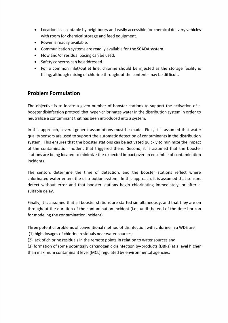
Criteria for location selection

Following criteria play an important role in proper selection of chlorine booster stations.

Location should be such that a relatively large volume of water can be disinfected.

The water to be treated travels in one direction.

The chlorine residual in water has begun to decrease but has not totally dissipated.

Chlorine can be applied uniformly in water.



Location is acceptable by neighbours and easily accessible for chemical delivery vehicles

with room for chemical storage and feed equipment.

Power is readily available.

Communication systems are readily available for the SCADA system.

Flow and/or residual pacing can be used. Safety concerns can be addressed.

For a common inlet/outlet line, chlorine should be injected as the storage facility is

filling, although mixing of chlorine throughout the contents may be difficult.

Problem Formulation

The objective is to locate a given number of booster stations to support the activation of a

booster disinfection protocol that hyper-chlorinates water in the distribution system in order toneutralize a contaminant that has been introduced into a system.

In this approach, several general assumptions must be made. First, it is assumed that water

quality sensors are used to support the automatic detection of contaminants in the distribution

system. This ensures that the booster stations can be activated quickly to minimize the impact

of the contamination incident that triggered them. Second, it is assumed that the booster

stations are being located to minimize the expected impact over an ensemble of contamination

incidents.

The sensors determine the time of detection, and the booster stations reflect where

chlorinated water enters the distribution system. In this approach, it is assumed that sensors

detect without error and that booster stations begin chlorinating immediately, or after a

suitable delay.

Finally, it is assumed that all booster stations are started simultaneously, and that they are on

throughout the duration of the contamination incident (i.e., until the end of the time-horizon

for modeling the contamination incident).

Three potential problems of conventional method of disinfection with chlorine in a WDS are

(1) high dosages of chlorine residuals near water sources;

(2) lack of chlorine residuals in the remote points in relation to water sources and

(3) formation of some potentially carcinogenic disinfection by-products (DBPs) at a level higher

than maximum contaminant level (MCL) regulated by environmental agencies.





different specified numbers of booster stations. Finally, trade-off curves between the total

disinfectant dose and the volumetric percentage of the water with residuals within a specified

range for different numbers of booster stations are obtained. Given a number of booster

stations nb, the mathematical formulation for the two-objective optimization problem is

b k n

i

n

k

k

i M f 1 1

1Minimize

100Maximaze

1

1

2

V

V

f

h mn

m

n

j

m

j

where

otherwise0

when ma xmin j

m j jh

m jm

j

ccct QV

where

f 1=total disinfectant dose;

f 2=percentage of the total volume of water supplied during a hydraulic cycle with residual

within specified limits;

Mi k=disinfectant mass (mg) added at booster station i in injection period k ;

V =total volume of demand over a hydraulic cycle;

Q j m

=demand at node j in monitoring period m;

t h=hydraulic (monitoring) time step;

c j m

=disinfectant concentration (mg/L) at monitoring node j and during monitoring interval

m; c j min

and c j max

=lower and upper bounds on disinfectant concentrations (mg/L) at

monitoring nodes;

=start of monitoring time;

nk =number of time steps in dosage cycle;

nh=number of time steps in hydraulic cycle (number of monitoring time steps); and

nm=number of monitoring nodes in which residual chlorine concentrations are controlled.

The aforementioned optimization problem is subject to the following constraints:

12C f

k b

k

i nk ni M ,...,1;,...,1;0



k

i

n

i

n

k

km

ij

m

j xcb k

1 1

1,...,;,...,1

max hm j

m

j nmn jcc

where

C 1=specified value representing Pareto optimal front for a range of f 2 greater than C 1;k

i x =multiplier of dosage rate at Booster i and during Injection Period k ;

km

ij =composite response of concentration at Node j and Monitoring Time m due to dosage

rate at Booster i and during Injection Period k .

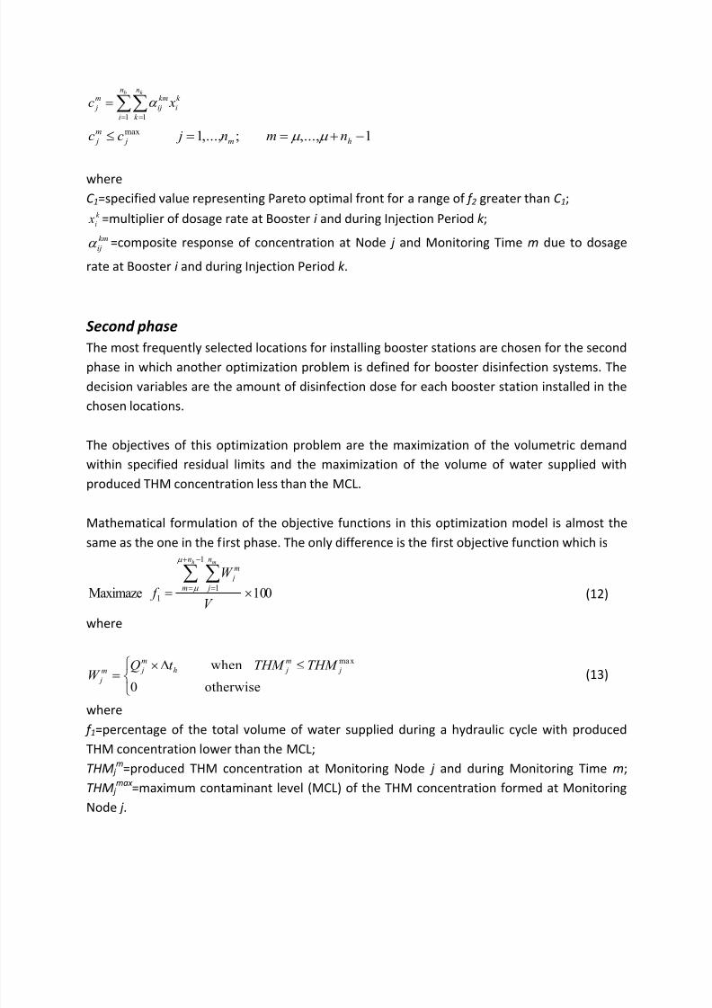
Second phase

The most frequently selected locations for installing booster stations are chosen for the secondphase in which another optimization problem is defined for booster disinfection systems. The

decision variables are the amount of disinfection dose for each booster station installed in the

chosen locations.

The objectives of this optimization problem are the maximization of the volumetric demand

within specified residual limits and the maximization of the volume of water supplied with

produced THM concentration less than the MCL.

Mathematical formulation of the objective functions in this optimization model is almost the

same as the one in the first phase. The only difference is the first objective function which is

100Maximaze

1

1

1

V

W

f

h mn

m

n

j

m

j

(12)

where

otherwise0

whenma x

j

m

jh

m

jm

j

THM THM t QW (13)

where

f 1=percentage of the total volume of water supplied during a hydraulic cycle with produced

THM concentration lower than the MCL;

THM j m

=produced THM concentration at Monitoring Node j and during Monitoring Time m;

THM j max

=maximum contaminant level (MCL) of the THM concentration formed at Monitoring

Node j .



Another constraint related to the first objective function is also added to the set of previous

constraints in this model:

21C f

where C 2=specified value representing Pareto optimal front for a range of f 1 greater than C 2.

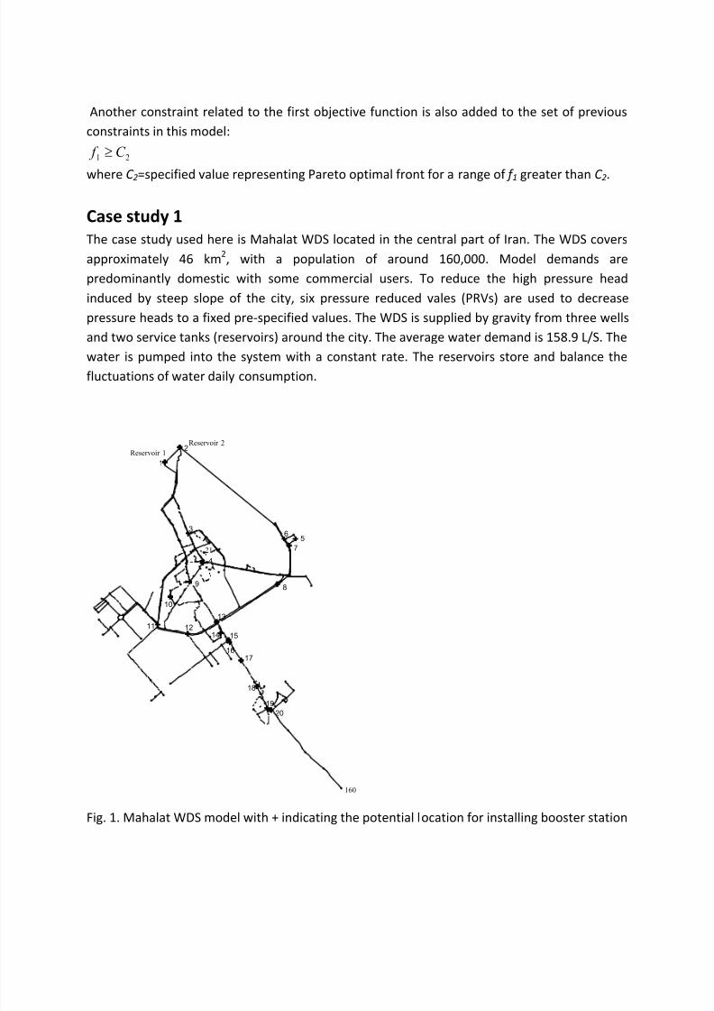
Case study 1

The case study used here is Mahalat WDS located in the central part of Iran. The WDS covers

approximately 46 km2, with a population of around 160,000. Model demands are

predominantly domestic with some commercial users. To reduce the high pressure head

induced by steep slope of the city, six pressure reduced vales (PRVs) are used to decrease

pressure heads to a fixed pre-specified values. The WDS is supplied by gravity from three wells

and two service tanks (reservoirs) around the city. The average water demand is 158.9 L/S. The

water is pumped into the system with a constant rate. The reservoirs store and balance the

fluctuations of water daily consumption.

Fig. 1. Mahalat WDS model with + indicating the potential location for installing booster station

1

2

3

4

56

7

89

10

11 12

13

14 15

16

17

18

19

20

160

21

Reservoir 1

Reservoir 2



Results and discussion

The multi-objective optimization problem of booster location and injection scheduling is

applied to Mahalat WDS model. Application of the model is carried out to assess

(1) the trade-off between the disinfectant dose and the percentage of safe drinking water(SDW) within specified residual limits;

(2) the trade-off between the percentage of SDW within specified residual limits and the

number of booster stations for a specified amount of total disinfectant dose; and

(3) the trace of THM concentration within WDS nodes with respect to optimal booster locations

and scheduling.

Two existing stations for chlorine injection are located at the water treatment plants

(reservoirs). If all of the nodes of the network are to be considered as potential locations, the

network setup would require a very high computational time and a large memory to storecumulative response coefficients. However, not all locations would be suitable due to

prohibitive costs, network hydraulics, and existing infrastructure. Therefore, 20 potential

locations including two existing locations and 18 potential boosters were assumed to be

available for installing booster station. These locations are shown in Fig. 1. Some of these

potential locations are located near the reservoirs, and the others are spread at critical points

throughout the network.

The value of C 1 is taken to be 75%. The hydraulics and booster injections are assumed to be

periodic with a period of 24 h. The water quality simulation duration is set to be 144 h and thefinal 24-h results are used in the calculation of composite response coefficients. Optimal trade-

off analyses were carried out using flow proportional type boosters due to their performance

rather than constant mass type boosters. A comparison is also made among the solutions with

varying numbers of booster locations.

Phase#1

In the first phase, the multi-objective optimization model is applied to find the trade-off

between the disinfectant mass and the percentage of SDW with the number of booster stations

as a third parameter. For flow proportional boosters, constant concentrations added at the

booster nodes are decision variables.

The maximum value of these variables is equal to 4.0 mg/L as the upper limit on residual

concentrations. It was observed that for nb< 4, 99.9% SDW could not be achieved. These curves

become almost flat after 99% SDW for nb≥ 4. The optimal trade-off curves indicate that the

SDW increases significantly with a small increase in the total dosage rate up to 95%. Then, the



marginal improvement in SDW with the increase in the dosage rate diminishes. Furthermore,

the improvement of SDW versus dosage rate is neglected for nb> 7

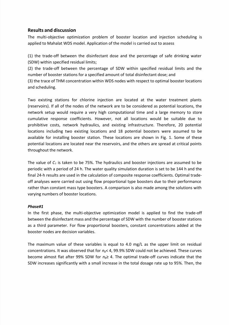
When limiting the budget of total disinfectant dose, Fig. 2(b) can be applied which shows the

trade-off between the variation of SDW and the number of boosters for different amount of total disinfectant dose. As it can be observed from this Fig., a significant increase in SDW can be

achieved for nb≤ 7.

It could be concluded from Fig. 2 that the optimal number of booster stations can be chosen

between four and seven, and the most efficiency can be achieved from seven optimal booster

stations. Although further considerations such as operational and budgetary limitations may

influence the final number chosen, seven booster stations seem to be the most efficient

number of booster stations from Figs. 2(a) and 2(b).

(a)(b)

Fig. 2. (a) Pareto fronts of total dosage versus percentage of SDW for different values of nb; (2)

Trade-off between percentage of SDW and number of boosters for different amounts of total

dosage



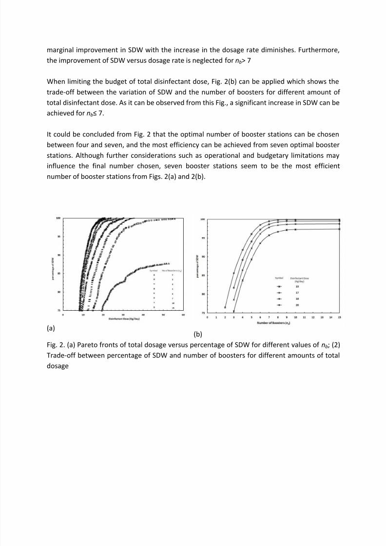
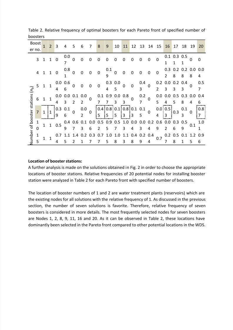
Table 2. Relative frequency of optimal boosters for each Pareto front of specified number of

boosters

Boost

er no.1 2 3 4 5 6 7 8 9 10 11 12 13 14 15 16 17 18 19 20

N u m b e r o f b o o s t e r s t a t i o n s ( n

b )

3 1 1 0 0.07

0 0 0 0 0 0 0 0 0 0 0 0.11

0.31

0.51

0 0

4 1 1 00.8

10 0 0 0

0.1

90 0 0 0 0 0

0.3

2

0.2

8

0.2

8

0.0

8

0.0

4

5 1 10.0

4

0.6

60 0 0 0

0.3

4

0.0

50 0

0.4

30

0.2

2

0.0

3

0.2

3

0.4

30

0.5

7

6 1 10.0

4

0.0

3

0.1

2

0.0

20

0.1

7

0.9

7

0.0

3

0.8

30

0.2

70

0.0

5

0.0

4

0.5

5

0.3

8

0.0

4

0.4

6

7 1 10.3

9

0.1

6

00.0

2

00.4

5

0.8

5

0.1

5

0.8

3

0.1

3

0.1

5

00.0

4

0.5

3

0.30.1

3

00.8

71

01 1 0.5

0.4

9

0.6

7

0.1

3

0.0

6

0.5

2

0.9

5

0.5

7

1.0

3

0.0

4

0.0

3

0.2

4

0.6

9

0.0

2

0.3

6

0.5

90.1

1.0

1

1

51 1

0.7

4

1.1

5

1.4

2

0.2

1

0.3

7

0.7

7

1.0

5

1.0

8

1.1

3

0.4

8

0.2

9

0.4

40.7

0.2

7

0.5

8

0.1

1

1.2

5

0.9

6

Location of booster stations:

A further analysis is made on the solutions obtained in Fig. 2 in order to choose the appropriate

locations of booster stations. Relative frequencies of 20 potential nodes for installing boosterstation were analyzed in Table 2 for each Pareto front with specified number of boosters.

The location of booster numbers of 1 and 2 are water treatment plants (reservoirs) which are

the existing nodes for all solutions with the relative frequency of 1. As discussed in the previous

section, the number of seven solutions is favorite. Therefore, relative frequency of seven

boosters is considered in more details. The most frequently selected nodes for seven boosters

are Nodes 1, 2, 8, 9, 11, 16 and 20. As it can be observed in Table 2, these locations have

dominantly been selected in the Pareto front compared to other potential locations in the WDS.



Case Study 2

Optimization for the location of chlorine booster stations in Al-Khobar water distribution

system, located on the eastern part of the Kingdom of Saudi Arabia, to determine the optimum

schedule of chlorine injection criteria for disinfectants was adopted, according to which the

minimum residual chlorine should not be less than 0.2 mg/l and greater than 4.0 mg/l.

Currently, in Al-Khobar water distribution system, there are three existing locations for the

injection of chlorine. For the purpose of selecting booster disinfection locations, thirty nodes in

the network are considered as potential booster locations. These nodes are selected based on

water quality simulation results. Some of the nodes are near the sources of water. Others are

selected based on the spatial behavior of these nodes. Some are selected in the areas having

the problem of low residual chlorine. The monitoring constraints should be satisfied at all the

consumer nodes.

There are some nodes that are neglected for monitoring constraints. These nodes are either the

groundwater reservoir or the nodes having zero demands. So, there is no need to fulfill the

condition of monitoring constraints at these locations. The model setup is the same as for the

existing design. The duration of water quality simulations is taken as 360 hours (15 days).

Results

The optimal results (location/scheduling) are obtained when the number of injection periods of

chlorine is 1 (1-24 h). The duration of the injection period is 24 hours. A constant concentration

of chlorine will be injected continuously at all the optimal booster stations for 24 hours

duration. The monitoring constraints for the residual chlorine are bounded between l = 0.2 mg/l

and u = 4.0 mg/l.

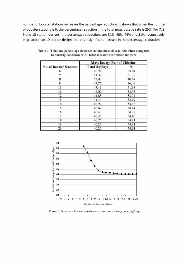
Table 1 and Figure 1 summarize the results of the study. They show the effect of the number of

booster stations on the total mass dosage rate. Figure 1 shows that the mass dosage rate

decreases as the number of booster stations increases. Then, at certain number of booster

stations, the amount of decrease in the mass dosage rate is not significant. The results indicate

that there is a considerable decrease in dosage rate up to 10 booster stations. After this, the

decrease in the dosage rate is insignificant. The mass dosage rate for the existing design is

89.272 kg/d.

The table shows the percentage decrease in the total mass dosage rate for the optimal results

when compared to the existing design. It can be observed from the table that increasing the



number of booster stations increases the percentage reduction. It shows that when the number

of booster stations is 6, the percentage reduction in the total mass dosage rate is 25%. For 7, 8,

9 and 10-station designs, the percentage reductions are 31%, 40%, 46% and 51%, respectively.

In greater than 10-station design, there is insignificant increase in the percentage reduction.



Conclusion

The results illustrate that a booster disinfection strategy can reduce considerably the amount of

chlorine required to maintain acceptable chlorine residual throughout the distribution system.

The important conclusions derived from this study are given below:

• The optimization results indicated that the booster disinfection efficiency can be maximized

by increasing the number of booster stations and the dosage duration. It can be concluded that

dosage reduction is a function of the number of booster stations and the number of scheduling

intervals.

• The results also showed that the considerable reduction in dosage rate, by increasing the

number of booster stations, is up to a certain limit; after this, the reduction is insignificant.

Documents

Optimal Location of Booster Chlorination Stations