Optimal Monetary Policy in a Phillips-Curve World ∗

Thomas F. Cooley

New York University

Vincenzo Quadrini

New York University

September 29, 2002

Abstract

In this paper we study optimal monetary policy in a model that integrates the modern

theory of unemployment with a liquidity model of monetary transmission. Two policy environ-

ments are considered: period by period optimization (time consistency) and full commitment

(Ramsey allocation). When the economy is subject to productivity shocks, the optimal policy

is pro-cyclical. We also characterize the long-term properties of monetary policy and show

that with commitment the optimal inflation rate is inversely related to the bargaining power

of workers. Both results find empirical support in the data.

Key words: Matching, unemployment, liquidity channel, time-consistent policy

JEL classification: E5, E6, J64

∗We thank Fabio Canova, Jordi Gali, Stephen LeRoy, Allan Meltzer and Shouyoung Shi for helpful comments

on earlier versions of this paper. We also thank workshop participants at Atlanta Fed, CEPR Summer Symposium,

Columbia University, Federal Reserve Board, NBER Summer Institute, New York University, Pompeu Fabra Uni-

versity, Richmond Fed, SED Meeting, University of California in San Diego, University of Chicago and University

of Rochester.

“Despite its disrepute within important academic and policymaking circles, the Phillips

Curve persists in U.S. data. Simple econometric procedures detect it.”

Thomas Sargent, 1998

Introduction

A robust empirical feature of post-war U.S. data is the positive correlation between inflation and

employment, which is commonly referred to as the Phillips curve relation (see Sargent (1998)).

This empirical feature supports the view that inflationary monetary policies have expansionary

effects on the real sector of the economy, at least in the short-run. The goal of this paper is

to study the optimal monetary policy in a model in which there is a direct link between these

policies and employment.

We study a general equilibrium model where the real side of the economy is characterized by a

search and matching framework with equilibrium unemployment. In this framework we introduce

a monetary sector in which changes in the supply of money affects the nominal interest rate by

changing the supply of loanable funds (liquidity effect). The change in the interest rate, in turn,

affects the financing cost of firms and impacts on the real sector of the economy. In this way the

model captures the “cost channel” of monetary transmission that Barth & Ramey (2001) find

significant for the propagation of monetary shocks. This channel is also consistent with recent

empirical studies that find significant liquidity effects of monetary policy shocks.1

We consider two policy environments. In the first environment we assume that monetary

policy interventions are decided on a period-by-period basis, and the monetary authority cannot

credibly commit to long-run plans (time-consistent policy). In studying the time-consistent policy,

we restrict the analysis to policies that are Markov-stationary, that is, policy rules that only

depend on the current (physical) states of the economy. In the second policy environment we

assume that the monetary authority is able to commit to long-term plans (Ramsey allocation).

1See, for example, Christiano, Eichenbaum, & Evans (1996), Leeper, Sims, & Zha (1996), Hamilton (1997).

1

There are two main findings. The first finding concerns the cyclical properties of the optimal

policy while the second concerns the long-term properties. Regarding the cyclical properties,

we show that in both policy environments the optimal policy is pro-cyclical when business cycle

fluctuations are driven by technology shocks: it increases the stock of money when employment

and output are high and reduces the stock of money when they are low. Further, the optimal

growth rate of money is positively correlated with employment and output. Both features—

the pro-cyclicality of the monetary aggregates and the money growth—characterize the post-war

history of the U.S. economy as documented in Cooley & Hansen (1995).

The second finding is that there are important differences between the long-term properties of

the time-consistent policy and the long-term properties of the optimal policy with commitment.

We show that when the worker’s share of the matching surplus is small and the employer’s share

high, the time-consistent policy is less inflationary than the optimal policy with commitment.

This result contrasts with earlier studies of optimal monetary policy, such as Kydland & Prescott

(1977) and Barro & Gordon (1983).

The intuition for these results is simple. Consider first the pro-cyclicality of the optimal policy.

After a positive productivity shock, the demand for loanable funds increases due to the firms’

desire to expand production. The increase in the demand for loanable funds raises the nominal

interest rate and this is inefficient. To prevent the interest rate increase, the policy maker has to

expand the supply of loanable funds by increasing the stock of money. Because the search and

matching frictions in the labor market generate a persistent response of employment to shocks

(hump-shaped response) and output grows for more than one period, the optimal growth rate

of money is above its steady state level for more than one period. This implies that the growth

rate of money is positively correlated with employment and output. In the absence of matching

frictions, however, output will grow only in the first period and then return to the steady state.

In this case the optimal growth rate of money would be negatively correlated with employment

and output: it would be below the steady state with the exception of the first period. Therefore,

the search and matching frictions are key to generating the pro-cyclicality of money growth.

2

Consider now the long-term properties of the optimal policy. In this economy there are two

possible sources of inefficiency. The first inefficiency derives from the cost of financing the current

production plan for firms. On this dimension a Friedman rule of a zero nominal interest rate is

optimal because a positive interest rate distorts the production decisions of firms by increasing

their financing cost. The second source of inefficiency derives from the matching frictions in the

labor market. As shown in Hosios (1990), if the worker’s share of the matching surplus is too small,

there will be an excessive creation of vacancies due to the high profitability of a match for the

firm. The policy maker can reduce the profitability of a match by increasing the nominal interest

rates. However, the decision to create new vacancies is not affected by the current interest rate

but only by future interest rates. The policy maker is able to credibly choose the future interest

rates only if it can commit. Otherwise, after the new vacancies have been created, it no longer

has the incentive to keep the high interest rate. The lack of commitment then implies that the

time-consistent policy is given by a simple Friedman rule of a zero nominal interest rate while the

optimal policy with commitment will set positive nominal interest rates. In the long run higher

interest rates are associated with higher inflation rates (Fisher rule). As will be shown in Section

5, the importance of the worker’s share of the surplus for the long-term property of the monetary

policy is supported by data for a cross-section of countries.

There are several studies that are related to this paper. Shi (1998) shows that with searching

frictions the Friedman rule may not be efficient, although he does not conduct an explicit analysis

of the optimal monetary policy. The optimal and time-consistent policy is studied in Ireland

(1996) but in an environment in which there are no frictions in the labor market and monetary

policy affects the real sector of the economy through the rigidity of nominal prices. In Ireland’s

model the optimal monetary policy is also pro-cyclical when business fluctuations are driven by

technology shocks. However, his results do not extend to our long-term results for which policy

commitment can affect the properties of the optimal policy. Our novel results depend crucially

on the consideration of search and matching frictions. A study of the differences between time-

consistent policies and optimal policies with commitment in models with sticky prices and liquidity

3

effects is conducted in Albanesi, Chari, & Christiano (1999). In contrast to our paper, they do not

find important long-term differences between the environment with and without commitment. We

reach a different conclusion because of the more complex dynamics introduced by the matching

frictions that characterize the labor market.

The plan of the paper is as follows. In section 1 we describe the model and in section 2

we define the optimal policy in the two policy environments: absence of commitment and full

commitment. Section 3 characterizes the analytical properties of the optimal policy and section

4 examines their quantitative properties. Section 5 discusses the empirical relevance of our long-

term results and provides cross-country evidence about the negative relation between the workers’

share of the surplus and the inflation rate. Finally, section 6 concludes.

1 The economy

We describe here a monetary economy that is specifically designed to generate the liquidity effect

of monetary interventions, that is a reduction in the nominal lending rate after a monetary

expansion. The reduction in the cost of borrowing, in turn, leads to an expansion in the real

sector of the economy. By designing the economy so that inflationary policies have expansionary

effects, we capture the main idea behind the Phillips curve relation—that is, the idea that in the

short run there is a trade-off between inflation and the real activity (a Phillips curve world)—and

this trade-off can be used for the design of monetary policy. The basic structure of the model is

similar to the one developed in Cooley & Quadrini (1999). In that paper, however, we did not

study the optimal policy which is the objective of the current paper.

1.1 The monetary authority and the intermediation sector

The total amount of households’ nominally denominated assets is denoted by M . We interpret

M as a broad monetary aggregate and will refer to it as money. Part of these assets are used for

transactions and the remaining quantity is held in the form of bank deposits. The funds collected

by banks are then used to make loans to firms. The monetary aggregate M is controlled by the

4

monetary authority by making transfers to the households in the form of bank deposits. The

monetary transfers are denoted by T = gM , where g is the growth rate of money.

For monetary interventions to have a liquidity effect—that is, a fall in the nominal interest

rate after a monetary expansion—some form of rigidity has to be imposed in the households’

ability to readjust their stock of deposits. We assume that the households choose the stock

of nominal deposits at the end of each period after all transactions have taken place and they

must wait until the end of the next period to change their portfolio. Denote by D the pre-

transfer household deposits. Because the monetary transfers are in the form of bank deposits

and households cannot readjust immediately these deposits, the funds available to banks to make

loans are D + gM . Therefore, an increase in the growth rate of money increases the stock of

loanable funds, which in turn induces a fall in the nominal interest rate. This is the liquidity

channel of “limited participation” models similar to Lucas (1990), Fuerst (1992) and Christiano

& Eichenbaum (1995).

1.2 Households

There is a continuum of agents of total measure 1 that maximize the expected lifetime utility:

E0

∞∑t=0

βt(ct − χta) (1)

where ct is consumption of market produced goods, a is the disutility from working and χt is an

indicator function taking the value of one if the agent is employed and zero if unemployed.

Households own three types of assets: transaction funds (cash), nominal deposits and firms’

shares. Denoting by m the pre-transfers nominally denominated assets and by d the quantity of

these assets kept in the form of deposits, the household’s transaction funds are m − d. In each

period, agents are subject to the following cash-in-advance and budget constraints:

P (c+ i) ≤ m− d (2)

5

P (c+ i) +m′ = m+ gM + (d+ gM)R+ χPw + Pπn (3)

The variable P is the nominal price, i is the household’s investment in the shares of new firms,

n identifies the number of firms’ shares that the household owns and π the real dividends paid

by these firms. The real wage received by an employed worker is denoted by w and it is paid

at the end of the period. The determination of the wage will be specified below. The nominal

after-transfer stock of deposits is d+ gM . These deposits earn the nominal interest rate R.

1.3 Production

The production sector is characterized by a search-matching framework similar to the labor-search

model of Pissarides (1988) and Mortensen & Pissarides (1994) with exogenous separation. The

production technology displays constant returns-to-scale with respect to the number of employees.

Without loss of generality, it is convenient to assume that there is a single firm for each worker.

The search for a worker involves a fixed cost κ and the probability of finding a worker depends on

the matching technology µV α(1 −N)1−α, where V is the number of vacancies (number of firms

searching for a worker), 1−N is the number of searching workers and α ∈ (0, 1). The probability

that a searching firm finds a worker is denoted by q and it is equal to µV α(1 − N)1−α/V ,

while the probability that an unemployed worker finds a job is denoted by h and is equal to

µV α(1 − N)1−α/(1 − N). Job separation is exogenous and occurs with probability λ. Workers

can search for a new job only if unemployed and there is no cost for searching.

If the searching process is successful, the firm operates the technology y = Axν , where A is

the aggregate level of technology and x is an intermediate input. Output goods and intermediate

goods are perfect substitutes, and therefore, the relative price is 1. The aggregate level of tech-

nology A is subject to shocks and follows a first order Markov process with transition density

function Γ(A,A′). The purchase of the intermediate good requires liquid funds. Firms get these

funds by borrowing from a financial intermediary at the nominal interest rate R.2

2In alternative, we could assume that working hours are flexible and the intermediate input is replaced by the

6

The contract signed between the firm and the worker specifies the wage w(s) which depends on

the states of the economy s. The set of aggregate states will be specified below. The determination

of the wage is such that the worker gets the share η of the matching surplus. The assumption of

a constant sharing fraction of the surplus is standard in this class of models and it is motivated

by assuming Nash bargaining between the firm and the worker, where η is the bargaining power

of the worker. As we will see later, this parameter plays a crucial role in characterizing the

properties of the optimal policy.

1.3.1 Firms

Firms post vacancies and implement optimal production plans to maximize the welfare of their

shareholders. Denote by J(s) the value of a match for the firm measured in terms of current

consumption. This is given by:

J(s) = π(s) + β(1− λ)EJ(s′) (4)

For notational convenience, we have defined the function π(s) = E(βP (s)/P (s′))π(s), where

π(s) are the dividends paid by the firm to the shareholders at the end of the period. The

function expresses the current value for the shareholder of the dividend paid by the firm. Because

dividends are paid at the end of the period, the shareholder needs to wait until the next period

to transform monetary payments into consumption. This implies that the real value (in terms of

today’s consumption) of one unit of money received at the end of the period is βP (s)/P (s′).

The dividends paid to the shareholders are equal to the output produced by the firm minus

the cost for the intermediate input, x(1 +R), and the labor cost, w:

π = Axν − x(1 +R)− w. (5)

number of working hours. The properties of the model would not change if we assume that the part of the worker’s

payment that compensates the disutility from working has to be paid in advance.

7

Notice that the cost for the intermediate input also includes the interest paid on the loan needed

to finance the payment of the input.

Given J(s) the firm’s value of a match as defined above, the value of a vacancy Q(s) is:

Q(s) = −κ+ q(s)βEJ(s′) + (1− q(s))βEQ(s′) (6)

Free entry implies that the value of a vacancy is zero in equilibrium and equation (6) becomes:

κ = q(s)βEJ(s′) (7)

Equation (7) is the arbitrage condition for the posting of new vacancies, and accordingly, for the

creation of new jobs. It simply says that the cost of posting a vacancy, κ, is in equilibrium equal

to the discounted expected return from posting the vacancy.

Consider now the worker. Define W (s, ϕ) and U(s) to be the values of being employed and

unemployed, in terms of current consumption. They are equal to:

W (s) = w(s)− a+ (1− λ)βEW (s′) + βλEU(s′) (8)

U(s) = h(s)βEW (s′) + (1− h(s))βEU(s′) (9)

where w(s) = E(βP (s)/P (s′))w(s). As with dividends, the wage w(s) is multiplied by the term

EβP (s)/P (s′) because wages are paid at the end of the period. Adding equations (4) to (8) and

subtracting (9) gives the total surplus generated by the match S(s). The surplus is shared between

the worker and the firm according to η, that is, W (s) − U(s) = ηS(s) and J(s) = (1 − η)S(s).

Using this sharing rule and equation (7), the surplus can be written as:

S(s) = π(s) + w(s)− a+(1− λ− ηh(s))κ

(1− η)q(s)(10)

8

Moreover, by equating W (s)− U(s) to ηS(s), and using (5), we derive the wage w(s) as:

w(s) = η(Axν − x(1 +R)) +(1− η)a

E(

βP (s)P (s′)

) +ηh(s)κ

q(s)E(

βP (s)P (s′)

) (11)

The wage w(s) as well as the surplus generated by the match depend on the intermediate

input x. Because the firm and the worker split the surplus, the optimal input maximizes this

surplus. The optimal input is then defined in the following proposition:

Proposition 1.1 The optimal input x is given by:

x =(

νA

1 +R

) 11−ν

Proof 1.1 The differentiation of the surplus in equation (10), after substituting π(s) + w(s) =

Axν − x(1 +R), gives the result. Q.E.D.

According to proposition 1.1, the intermediate input—and therefore, the firm’s output—

is decreasing in the nominal interest rate R. This is because the interest rate increases the

marginal cost of the intermediate input. This is the direct channel through which monetary

policy interventions impact on the real sector of the economy. This is in addition to the dynamic

impact that will affect employment as described below.

Using equations (7) and (4) we derive:

κ

q(s)= βπ(s′) + βE

((1− λ)κq(s′)

)(12)

where π(s) is the value in terms of current consumption of dividends distributed by the firm at

the end of the period. Using forward substitution and the law of iterated expectations we have:

κ

q(st)= βEt

∞∑j=1

[β(1− λ)]j−1π(st+j) (13)

9

Because κ is constant, an increase in the expected sum of future dividends (properly dis-

counted) induces a reduction in the current value of q, that is, the probability that a vacancy

is filled. The fall in q requires an increase in the number of vacancies which in turn increases

the next period employment. Equation (13) provides intuition on how changes in the interest

rate affect the employment rate. If a fall in the future interest rates generates an increase in

the expected dividends, it will induce an increase in employment. Also notice that the future

inflation rates play an important role as πt+j = βPt+jπt+j/Pt+j+1, for j ≥ 1. On the other hand,

the current dividend πt and the next period inflation rate Pt+1/Pt do not enter equation (13).

These observations are key to understanding the different properties of the optimal policies

with and without commitment. These policies will be characterized in detail in later sections.

Here, we would like to provide some intuition about the differences. Without commitment,

the policy maker is unable to (credibly) determine the future inflation and interest rates. This

implies that the policy maker is unable to affect employment. With commitment, instead, the

policy maker can affect employment because it can (credibly) choose the future policies today.

Consequently, if the equilibrium employment is not efficient, we would expect that the optimal

policy with commitment differs from the time-consistent policy.

2 Defining the optimal monetary policy

We can now define the optimal monetary policy under the two policy regimes. We begin with

the case where commitment is not possible.

2.1 Optimal and time-consistent monetary policy

In this section we define the optimal policy when the monetary authority chooses the growth

rate of money on a period-by-period basis and cannot credibly commit to the choice of future

rates. We restrict the analysis to policies that are Markov stationary, that is, policy rules that

are functions of the current aggregate states of the economy. Given s the current states, a policy

rule will be denoted by g = Ψ(s).

10

The procedure we follow to derive the time-consistent policy consists of two steps. In the

first step we define a recursive equilibrium where the policy maker follows an arbitrary policy

rule Ψ(s). In the second step we ask what the optimal growth rate of money should be today if

the policy maker anticipates that from tomorrow on it will follow some arbitrary rule Ψ(s). This

allows us to derive the optimal current g as a function of the current states and the arbitrary

future rule. We denote the function that returns the optimal current policy by g = ψ(Ψ; s). If

the current policy rule ψ is equal to the policy rule that will be followed from tomorrow on, that

is, ψ(Ψ; s) = Ψ(s) for all s, then Ψ is an optimal and time consistent policy rule. We describe

these two steps in detail in the next two subsections.

2.1.1 The household’s problem given the policy function Ψ

Assume that the policy maker commits to the policy rule g = Ψ(s). Then, using a recursive

formulation, we describe the household’s problem and define a competitive equilibrium conditional

on this policy rule. In order to use a recursive formulation, we normalize all nominal variables by

the pre-transfer stock of money M . The aggregate states of the economy are the aggregate level

of technology, A, the normalized pre-transfer stock of nominal deposits, D, and the number of

employed workers, N. Therefore, s = (A,D,N). The individual states are the occupational status

χ, the normalized pre-transfer stock of nominally denominated assets m, the normalized pre-

transfer stock of nominal deposits d, and the number of firms’ shares n owned by the household.

We denote the set of individual states by s = (χ,m, d, n). The household’s problem is:

Ω(Ψ; s, s) = maxn′,d′

c− χa+ β E Ω(Ψ; s′, s′)

(14)

subject to

c ≤ m− d

P− (n′ − (1− λ)n)κ

q(15)

11

m′ =(d+ g)(1 +R) + P (χw + nπ)

(1 + g)(16)

s′ = H(Ψ; s) (17)

g = Ψ(s) (18)

Notice that in order to have n′ shares of active firms in the next period, the household buys

(n′ − (1− λ)n) new shares. Given the matching probability for a new vacancy, q, the creation of

a new firm requires the posting of 1/q new vacancies, each of which costs κ. Therefore, the total

investment in new firm shares is i = (n′ − (1 − λ)n)κ/q. In solving this problem, the household

takes as given the policy rule Ψ and the law of motion for the aggregate states H defined in

equation (17). To make clear that this problem is conditional on the particular policy rule Ψ,

this function has been included as an extra argument in the household’s value function and in

the aggregate law of motion.

A solution for this problem is given by the state contingent functions n′(Ψ; s, s) for next period

firms’ shares and d′(Ψ; s, s) for bank deposits. As for the value function, we make explicit the

dependence of these decisions on the policy rule Ψ.

In equilibrium, households are indifferent about the allocation of liquid funds (money) be-

tween the purchase of consumption goods and the purchase of firms’ shares, independently of

their employment status. This derives from the assumption that the utility function is linear

in consumption. Because the aggregate behavior of the economy is independent of the distribu-

tions of firms’ shares among households, we concentrate on the symmetric equilibrium in which

all agents make the same portfolio choices of deposits and shares of firms. This implies that

differences in earned wages between employed and unemployed workers give rise to different con-

sumption levels rather than differences in asset holdings. We then have the following definition.

Definition 2.1 (Symmetric equilibrium given Ψ) A recursive symmetric competitive equi-

12

librium, given the policy rule Ψ, is defined as a set of functions for (i) household decisions

n′(Ψ; s, s), d′(Ψ; s, s), and value function Ω(Ψ; s, s); (ii) intermediate input x(Ψ; s); (iii) wage

w(Ψ; s); (iv) loans L(Ψ; s); (v) interest rate R(Ψ; s) and nominal price P (Ψ; s); (vi) law of mo-

tion H(Ψ; s). Such that: (i) the household’s decisions are optimal solutions to the household’s

problem (14); (ii) the intermediate input x maximizes the surplus of the match; (iii) the wage is

such that the worker obtains a fraction η of the surplus; (iv) the market for loans clears, that is

D + g = L(Ψ; s), and R(Ψ; s) is the equilibrium interest rate; (v) the law of motion H(Ψ; s) for

the aggregate states is consistent with the individual decisions of households and firms; (vi) all

agents choose the same holdings of deposits and firms shares (symmetry).

Differentiating the objective function (14) with respect n′, we get:

κ

q= β E

(βP ′π′

P ′′(1 + g′)

)+ β E

((1− λ)κ

q′

)(19)

which is equivalent to (12) derived before. The first order condition with respect to d′ is:

E

(1P ′

)= βE

(1 +R′

P ′′(1 + g′)

)(20)

which is the Euler equation in standard dynamic models with money when agents are risk neutral.

2.1.2 One-shot optimal policy and the fixed point of the policy problem

In the previous subsection we derived the household’s decision rules n′(Ψ; s, s) and d′(Ψ; s, s),

and the value function Ω(Ψ; s, s) for a given policy rule Ψ. We now ask what the optimal policy

would be today, if the policy maker anticipates that from tomorrow on it will follow an arbitrary

policy rule Ψ. Defining the optimality of a particular policy requires the definition of a welfare

objective. Our assumption is that the policy maker attributes equal weight to all households

independently of their employment status.

To determine the optimal growth rate of money today, we need to derive a function that links

13

the households’ welfare to g. To derive this function, we first consider the following household’s

problem:

V (Ψ; s, s, g) = maxn′,d′

c− χa+ β E Ω(Ψ; s′, s′)

(21)

subject to

c ≤ m− d

P− (n′ − (1− λ)n)κ

q(22)

m′ =(d+ g)(1 +R) + P (χw + nπ)

(1 + g)(23)

s′ = H(Ψ; s, g) (24)

where Ω(Ψ; s′, s′) is the next period value function conditional on the policy rule Ψ derived in

the previous section. The new function V (Ψ; s, s, g) is the value function for the household when

the current growth rate of money is g and future growth rates are determined according to the

policy rule Ψ.

After solving this problem and imposing the aggregate consistency condition in the symmetric

equilibrium m = M = 1, d = D, and n = N , the objective function of the policy maker can be

written as:

V(Ψ; s, g) = N · V (Ψ; s, 1,M,D,N, g) + (1−N) · V (Ψ; s, 0,M,D,N, g) (25)

which is simply the weighted average of the value functions for employed and unemployed house-

holds. The unemployment status is the only source of heterogeneity because we are restricting

the competitive equilibrium to be symmetric in the sense that all the households choose the same

level of assets (but different consumption). The policy maker chooses g to maximize the above

14

objective, that is,

gOPT = arg maxg

V(Ψ; s, g) = ψ(Ψ; s) (26)

We then have the following definition of an optimal and time-consistent monetary policy rule.

Definition 2.2 The optimal and time-consistent monetary policy rule ΨOPT (s) is the fixed point

of the mapping ψ(Ψ; s), that is:

ΨOPT (s) = ψ(ΨOPT ; s)

The basic idea behind this definition is that, when the agents in the economy (households,

firms and the monetary authority) expect that future values of g are determined according to the

policy rule ΨOPT , the optimal value of g today is the one predicted by the same policy rule ΨOPT

that will determine the future values. This property assures that the policy maker will continue

to use the same policy rule in the future, so it is rational to assume that future values of g will

be determined by this rule.

2.2 Optimal policy with commitment

With commitment, the policy maker chooses at time zero a sequence of money growth as a function

of future history realizations of the shock and the initial states. The equilibrium allocation

associated with this policy is usually referred to as the Ramsey equilibrium.

Let ht be the history of shock realizations from time zero up to time t and let Ht be the

collection of all possible histories. A monetary policy with commitment can be expressed as

gt = g(N0,ht), for all ht ∈ Ht and t ≥ 0. Similarly, the realization of the interest rate induced

by this policy can be expressed as a function of N0 and ht, that is, Rt = R(N0,ht). The policy

maker will choose g(N0,ht) to maximize the expected discounted utility of the representative

household obtained under the competitive allocation induced by the policy g(N0,ht). If we define

C(N0,ht|g(N0,ht)) the aggregate consumption induced by the policy g(N0,ht) in the competitive

equilibrium and N(N0,ht|g(N0,ht)) the employment rate also induced by the policy g(N0,ht) in

15

the competitive equilibrium, the optimal policy with commitment is defined as:

arg maxg(N0,ht)ht∈Htt≥0

E0

∞∑t=0

βt[C(N0,ht|g(N0,ht))− aN(N0,ht|g(N0,ht))

](27)

The characterization of the optimal policy follows the primal approach and consists of choosing

the optimal allocation among the set of all competitive allocations induced by a feasible policy

g(N0,ht). See Chari, Christiano, & Kehoe (1996) for details about the primal approach.

3 Properties of the optimal policy

Before characterizing the properties of the optimal policy, let’s observe that for a given aggregate

stock of deposits, there is a simple relation between the nominal interest rate and the current

growth rate of money. This is formally established in the following lemma.

Lemma 3.1 Given the aggregate stock of deposits, the nominal interest rate is equal to R =

max

ν(1+g)D+g − 1 , 0

.

Proof 3.1 Appendix.

Although we have defined the monetary policy in terms of the growth rate of money, Lemma

3.1 implies that a definition in terms of the interest rate would induce the same real allocation

(employment and consumption). The next two subsections characterize the properties of the

optimal monetary policy in the two policy environments.

3.1 Optimal policy without commitment

We have the following proposition.

Proposition 3.1 (Policy without commitment) If there is not commitment, the optimal pol-

icy maintains the nominal interest rate to zero in any state of the economy.

16

Proof 3.1 Appendix.

Therefore, the Friedman rule of a zero nominal interest rate is the optimal policy when the

policy maker cannot commit to future policies. This result is also obtained in Albanesi et al.

(1999) and depends on the fact that the current growth rate of money does not affect future

employment. Future employment will be affected by future growth rates of money but without

commitment the policy maker is unable to choose credibly these rates. Given the inability to

affect future employment, the optimal policy will choose a current growth rate of money that

leads to a zero interest rate. This is because a zero interest rate does not distort the production

choice of the existing matches, that is, the choice of the intermediate input.

Although the time-consistent policy gives a precise prediction about the nominal interest rate,

a zero interest rate can be implemented with a multiplicity of growth rates of money (see Lemma

3.1). The policy indeterminacy (in terms of money growth) derives from the fact that with a zero

nominal interest rate the cash-in-advance constraints of households and firms are not binding and

several sequences of money growth can induce a zero interest rate. In what follows we restrict

the analysis to a particular policy, that is, the policy under which the whole quantity of money is

used for transaction. The following proposition characterizes the optimal growth rate of money

in the environment without policy commitment and full use of money.

Proposition 3.2 (Procyclical time-consistent policy) Without policy commitment, the op-

timal growth rate of money compatible with full use of money is given by g = βE−1(1 + gY )− 1,

where E−1(1 + gY ) is the expected gross growth rate of output before the observation of the shock.

Proof 3.2 Appendix.

Therefore, the growth rate of money depends only on the predictable part (before the shock)

of the growth rate of output and current (unpredictable) productivity shocks do not affect the

optimal growth rate of money. This is because in the current period the nominal interest rate is

17

determined by the equilibrium condition R = ν(1+ g)/(D+ g)− 1 (see Lemma 3.1). Because the

stock of deposits D cannot be changed, the constancy of R requires the constancy of g.

The fact that the optimal growth rate of money follows the predictable growth rate of output

implies that the growth rate of money is pro-cyclical if the growth rate of output displays some

persistence. In this respect the matching frictions play an important role in the model. In a

limited participation model with a neoclassical production technology—and therefore, absence of

matching frictions—the response of output to shocks is not hump-shaped. This implies that in

this latter model the growth rate of output is positive only in the first period. Because in the

first period the increase in output is not expected, the growth rate of money does not change.

After the first period the growth rate of output becomes negative because it converges back to

the steady state and the growth rate of money will be negative. This implies that when output

is above the steady state, the growth rate of money is negative (counter-cyclical). The matching

framework, instead, is able to generate a hump-shaped response of output as shown in Merz

(1995), Andolfatto (1996) and Den-Haan, Ramey, & Watson (2000). Consequently, output will

continue to growth beyond the first period which induces an increase in the optimal growth rate

of money in the first few periods. As we will see in Section 4, this generates a pro-cyclical response

of the growth rate of money.

3.2 Optimal policy with commitment

We have the following proposition.

Proposition 3.3 (Policy with commitment) If η ≥ 1 − α, the optimal policy with commit-

ment implies R(N0,ht) = 0 for all t = 0, 1, 2, ... (Friedman rule). If η < 1− α the optimal policy

with commitment implies R(N0,h0) = 0 and R(N0,ht) > 0 for some t ≥ 1.

Proof 3.3 Appendix.

According to this proposition, if the worker’s share of the surplus η is too small, the optimal

policy with commitment induces positive interest rates. Therefore, in contrast to the case without

18

commitment, the Friedman rule of a zero nominal interest rate is not optimal unless the bargaining

power of the worker is sufficiently large.

To understand these properties, we have to consider the two channels through which monetary

policy affects the real sector of the economy: the direct channel and the indirect channel. The

direct channel works through the cost of financing the intermediate input x. Given the number of

employed workers, a higher interest rate increases the financing cost of the firm and reduces pro-

duction. On this dimension, a zero nominal interest rate would be optimal. The indirect channel

works through the incentives to create vacancies. The policy maker can increase employment by

reducing the profitability of a match. This, in turn, can be obtained by increasing the inflation

and interest rates. Therefore, if the employment rate is not efficient under a Friedman rule, the

policy maker may deviate from this rule. More precisely, if the worker’s share of the surplus

η is smaller than 1 − α, the Hosios (1990) conditions for the efficiency of the matching process

are violated, and the high profitability of a match for the firm induces an excessive creation of

vacancies. Under this condition the policy maker would like to reduce job creation. However, the

decision to create new vacancies is not affected by either the current interest rate or the current

inflation rate. What affects the return on a new vacancy are the future interest and inflation

rates. This can be seen from equation (13) which for simplicity we rewrite below:

κ

q(s0)= βE0

∞∑t=1

[β(1− λ)]t−1π(st)βP (st)P (st+1)

(28)

The infinite sum on the right hand side of this equation starts at t = 1. This implies that the

creation of new vacancies at time zero does not depend on the current interest rate and the current

and next period inflation rates (change in prices between today and tomorrow). Consequently,

the optimal growth rate of money in the current period will be set such that R0 = 0. Future

inflation and growth rates of money, instead, will be set taking into consideration the possibility

of correcting for the second source of inefficiency. Under the condition η < 1− α, this requires a

higher average inflation rate which induces a higher average nominal interest rate. If η > 1− α,

19

it would be optimal to have negative interest rates. A negative interest rate, however, is not

compatible with a competitive equilibrium.

With shocks the full characterization of the commitment policy is not available. In general,

we would not expect that the interest rate is constant over the business cycle because the trade-off

between the production efficiency (the optimal input x) and the optimal employment is affected

by the shock. However, we would expect that the average interest and inflation rates are higher

when η < 1 − α. This will be shown numerically in Section 4. In that section we will also show

the numerical cyclical properties of the commitment policy.

3.3 Optimal policy with externality

The analysis of the previous two subsections showed that without commitment the optimal policy

maintains a zero interest rate and a negative inflation rate. This would also be the optimal policy

with commitment when η ≥ 1 − α. We now introduce an extra feature that allows for the

optimality of a positive long-term interest rate even if there is no commitment but it does not

change the basic cyclical (short-term) properties of the optimal policy. We assume that each firm

generates a negative externality of the form ξ · Axν , where ξ is constant. With this externality,

propositions 3.1 and 3.2 become:

Proposition 3.4 (Policy without commitment) If there is not commitment, the optimal pol-

icy maintains the nominal interest rate equal to ξ/(1 − ξ) in any state of the economy and

g = βE−1(1 + gY )/(1− ξ)− 1.

Proof 3.4 The proof follows the same steps of propositions 3.1 and 3.2 taking into account the

externality ξAXνN in the objective of the policy maker. Q.E.D.

The introduction of the externality is also important to differentiate the long-term properties

of the optimal policy without commitment. Proposition 3.3 becomes:

20

Proposition 3.5 (Policy with commitment) If η = 1 − α the commitment policy implies

R(N0,ht) = ξ/(1− ξ) for all t = 0, 1, 2, ... (constant interest rate). If η < 1− α the commitment

policy implies R(N0,h0) = ξ/(1− ξ) and R(N0,ht) > ξ/(1− ξ) for some t ≥ 1. If η > 1− α the

commitment policy implies R(N0,h0) = ξ/(1− ξ) and R(N0,ht) < ξ/(1− ξ) for some t ≥ 1.

Proof 3.5 The proof follows the same steps of propositions 3.3 taking into account the externality

ξAXνN in the objective of the policy maker. Q.E.D.

Although it is still the case that commitment may increase inflation when η is small, for large

values of η the opposite may be true as we will show numerically in the next section. Therefore,

our results are qualitatively similar to the results of Kydland & Prescott (1977) and Barro &

Gordon (1983) if η is large but they differ if η is small. We will come back to this point in Section

5 when we discuss the empirical plausibility of the condition η < 1 − α and the evidence about

the relationship between commitment and inflation.

4 Quantitative properties of the optimal policy

In this section we analyze the quantitative properties of the optimal monetary policy (with and

without commitment). Our analysis will be focused on the properties of the economy around

the steady state. In the regime with policy commitment the steady state is the equilibrium to

which the economy will converge after the initial implementation of the optimal plan in absence

of shocks. The problem solved to characterize the limiting equilibrium with policy commitment

is described in Appendix E.

4.1 Calibration

The model is calibrated to U.S. data. The period is one quarter and the discount factor is

β = 0.99. The parameter ξ is chosen to get a steady state quarterly interest rate equal to

0.018. This implies a steady state inflation rate of about 0.008 per quarter. The value of ξ

needed to obtain an interest rate equal to 0.018 depends on the policy regime. In the regime

21

without commitment we set ξ = 0.017682. As stated in proposition 3.4 this will guarantee

that the equilibrium interest rate is equal to the calibration target. In the regime with policy

commitment the value of ξ depends on the whole set of parameters. In the baseline model we

set ξ = 0.0034977. Approximately, this implies that policy commitment increases the long-term

inflation rate by about 0.014 per quarter (about 6 percent per year).

The production function is characterized by the parameter ν and the stochastic properties

of the shock. The nominally denominated assets used by households for transaction purposes

(money) as a fraction of their total nominally denominated assets, is equal to (M −D)/M(1+g).

This can also be written as (1− ν) +RD/M(1 + g).3 Because RD/M(1 + g) is a small number,

we take 1− ν to be the approximate fraction of transaction funds used by households. A proxy

for 1− ν is then given by the stock of M1 used by households as a fraction of M3 that they own.

The value chosen is ν = 0.85.

The aggregate level of technology A follows the first-order autoregressive process log(A′) =

ρlog(A) + ε′, with ε ∼ N(0, σ2). The parameter ρ is assigned the value 0.95, and σ is set such

that the volatility of output generated by the model in the regime without commitment is similar

to the data. The value chosen is σz = 0.0009. Of course, the evaluation of the model will not be

based on the ability to match the volatility of output.

The workers share of the surplus is set to η = 0.2. This is about half the value that would

guarantee an efficient creation of new vacancies. After fixing η, the disutility from working, a, is

chosen so that the steady state capital income share is 18 percent. This value guarantees that the

net capital income share (net of depreciation) is similar to the data.4 To evaluate the importance

of η, we will report the simulation results also for other values of this parameter.

3This is obtained by using M −D = PC = P (1− ν)Y + RD and PY = M(1 + g).

4In standard models the gross capital income share is higher (about 35%) because it compensates for the higher

depreciation of capital. In our economy, the only accumulation of capital comes from the initial cost of creating new

vacancies. Consequently, the aggregate stock of capital and its replacement are smaller than in standard models.

22

The searching and matching section of the model is characterized by four parameters: the

parameters of the matching technology, µ and α, the probability of exogenous separation, λ, and

the cost of creating a new vacancy, κ. We set α = 0.6 which is consistent with the estimate of

Blanchard & Diamond (1989). Then to calibrate the parameters µ, λ and κ, we follow Andolfatto

(1996) and impose the following steady state targets: (a) the fraction of the population that is

employed equals 0.57;5 (b) the probability that a vacancy is successfully filled is q = 0.9; and (c)

the transition probability from employment to non-employment is λ = 0.15.

4.2 Cyclical properties of the calibrated economy

Figure 1 plots the impulse responses of several variables to a positive productivity shock under

the policy regimes with and without commitment. The figure also plots the impulse responses

under two alternative regimes. In the first regime the policy maker keeps the growth rate of

money constant (passive policy) while in the second regime it controls the nominal interest rate

according to the following specification of the Taylor rule:

Rt = R+ γy(Yt − Y ) + γp(Pt − Pt−1) (29)

where Rt is the nominal interest rate, Yt is logarithm of aggregate output, Pt is the logarithm of

the price level and the bar sign denotes steady state values. As suggested in Taylor (1998), we

5This implies that the steady state fraction of searching workers is 0.43. Here we are adopting is broader

definition of searching workers which includes not only unemployed workers but also individuals that are out of the

labor force. This captures the fact that some of the new hired workers do not transit through the pool of formally

defined unemployed workers. From a technical point of view, this larger fraction is important because is reduces

the impact that changes in the number of employed workers have on the probability that an advertised vacancy is

filled. When the fraction of steady state searchers is small, a small percentage increase in the number of employed

workers corresponds to a large percentage fall in the number of searching workers, which in turn implies a large

fall in the probability with which new vacancies are filled.

23

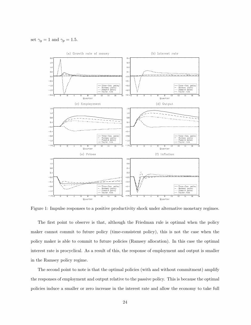
set γy = 1 and γp = 1.5.

Figure 1: Impulse responses to a positive productivity shock under alternative monetary regimes.

The first point to observe is that, although the Friedman rule is optimal when the policy

maker cannot commit to future policy (time-consistent policy), this is not the case when the

policy maker is able to commit to future policies (Ramsey allocation). In this case the optimal

interest rate is procyclical. As a result of this, the response of employment and output is smaller

in the Ramsey policy regime.

The second point to note is that the optimal policies (with and without commitment) amplify

the responses of employment and output relative to the passive policy. This is because the optimal

policies induce a smaller or zero increase in the interest rate and allow the economy to take full

24

advantage of the higher productivity. On the other hand, the failure to increase the growth rate of

money in the passive policy induces an increase in the interest rate which dampens the response

of the economy to the shock. When the policy maker follows the Taylor rule, the aggressive

counter-cyclical properties of this rule goes beyond restricting the response of employment and

output and generates a recession. We should point out, however, that in our specification of the

Taylor rule we have assumed that potential output is constant. If we allow potential output to

depend on the shock, the stabilization consequences of this rule would be smaller.

Table 1 reports some business cycle statistics computed from the simulation of the artificial

economy. As expected from the impulse responses plotted in Figures 1 (panel (c) and (d)), the

volatility of employment and output is larger under the optimal policy regimes. Under these

regimes the model generates volatility of money stock and money growth that are not very

different from the data. It also generates positive correlations of the stock of money and the

growth rate of money with employment and output. Employment is also positively correlated

with the inflation rate. The correlation of inflation and output is positive although it is close to

zero. Nevertheless, this is an important improvement compared to the other two policy regimes

that generate a negative correlation. To explain why the optimal policy improves the performance

of the model along this dimension, consider first the case of a passive policy. In this regime, when

output expands prices fall and when output contracts prices increase. As shown in the first panel

of Figure 1, in the optimal policy regime the price level falls only in the first period of the shock.

But in the first period the growth in output is small relative to the subsequent growth (see panel

(d) of Figure 1). Another important feature of the model is the autocorrelation of the optimal

growth rate of money as reported in the lower section of the table. This autocorrelation is positive

and close to the value found in the data.

It is important to emphasize that the positive correlation of employment and output with the

optimal growth rate of money depends crucially on the fact that the response of output to shocks is

hump-shaped. The hump-shaped response occurs because of the searching and matching frictions.

Without these frictions, the response of output would not be hump-shaped and the growth rate

25

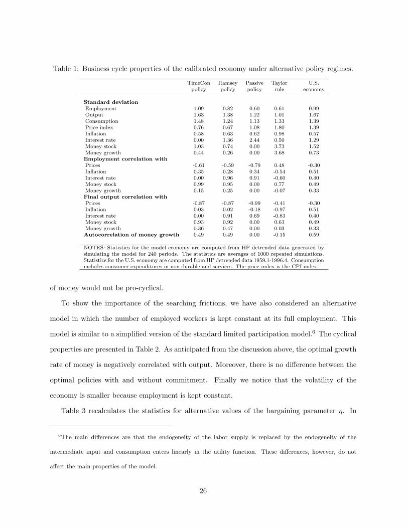
Table 1: Business cycle properties of the calibrated economy under alternative policy regimes.

TimeCon Ramsey Passive Taylor U.S.policy policy policy rule economy

Standard deviationEmployment 1.09 0.82 0.60 0.61 0.99Output 1.63 1.38 1.22 1.01 1.67Consumption 1.48 1.24 1.13 1.33 1.39Price index 0.76 0.67 1.08 1.80 1.39Inflation 0.58 0.63 0.62 0.98 0.57Interest rate 0.00 1.36 2.44 0.50 1.29Money stock 1.03 0.74 0.00 3.73 1.52Money growth 0.44 0.26 0.00 3.68 0.73Employment correlation withPrices -0.61 -0.59 -0.79 0.48 -0.30Inflation 0.35 0.28 0.34 -0.54 0.51Interest rate 0.00 0.96 0.91 -0.60 0.40Money stock 0.99 0.95 0.00 0.77 0.49Money growth 0.15 0.25 0.00 -0.07 0.33Final output correlation withPrices -0.87 -0.87 -0.99 -0.41 -0.30Inflation 0.03 0.02 -0.18 -0.97 0.51Interest rate 0.00 0.91 0.69 -0.83 0.40Money stock 0.93 0.92 0.00 0.63 0.49Money growth 0.36 0.47 0.00 0.03 0.33Autocorrelation of money growth 0.49 0.49 0.00 -0.15 0.59

NOTES: Statistics for the model economy are computed from HP detrended data generated bysimulating the model for 240 periods. The statistics are averages of 1000 repeated simulations.Statistics for the U.S. economy are computed from HP detrended data 1959.1-1996.4. Consumptionincludes consumer expenditures in non-durable and services. The price index is the CPI index.

of money would not be pro-cyclical.

To show the importance of the searching frictions, we have also considered an alternative

model in which the number of employed workers is kept constant at its full employment. This

model is similar to a simplified version of the standard limited participation model.6 The cyclical

properties are presented in Table 2. As anticipated from the discussion above, the optimal growth

rate of money is negatively correlated with output. Moreover, there is no difference between the

optimal policies with and without commitment. Finally we notice that the volatility of the

economy is smaller because employment is kept constant.

Table 3 recalculates the statistics for alternative values of the bargaining parameter η. In

6The main differences are that the endogeneity of the labor supply is replaced by the endogeneity of the

intermediate input and consumption enters linearly in the utility function. These differences, however, do not

affect the main properties of the model.

26

Table 2: Business cycle properties of the calibrated economy without matching frictions.

TimeCon Ramsey Passive Taylor U.S.policy policy policy rule economy

Standard deviationOutput 0.77 0.77 0.76 1.53 1.67Consumption 0.86 0.86 0.85 1.72 1.39Price index 0.76 0.76 0.67 9.83 1.39Inflation 0.58 0.58 0.61 2.02 0.57Interest rate 0.00 0.00 1.61 1.63 1.29Money stock 0.14 0.14 0.00 13.84 1.52Money growth 0.01 0.01 0.00 4.67 0.73Final output correlation withPrices -0.98 -0.98 -0.98 -0.32 -0.30Inflation -0.88 -0.88 -0.32 -0.80 0.51Interest rate 0.00 0.00 0.69 -0.75 0.40Money stock 0.14 0.14 0.00 0.33 0.49Money growth -0.70 -0.70 0.00 -0.75 0.33

NOTES: Statistics for the model economy are computed from HP detrended data generatedby simulating the model for 240 periods. The statistics are averages of 1000 repeated simula-tions. Statistics for the U.S. economy are computed from HP detrended data 1959.1-1996.4.Consumption includes consumer expenditures in non-durable and services. The price indexis the CPI index.

changing η we also change three other parameters: the working disutility a, the externality

parameter ξ in the regime with policy commitment, and the standard deviation of the shock

σz. The new working disutility is such that there is no change in the steady state capital income

share. The change in the externality parameter in the regime with policy commitment guarantees

that the steady state interest rate does not change. The new standard deviation of the shock

guarantees that the volatility of output in the regime without commitment remains the same.

A brief inspection of Table 3 shows that for η < 1−α policy commitment reduces the volatility

of employment and output relative to the regime without commitment. However, when η > 1−α,

the reverse seems to be true. This is because in this case the optimal response of the interest rate

under commitment tends to be counter-cyclical (it decreases during an expansion and increases

during a recession). In fact, the correlation of employment and output with the interest rate is

positive for η = 0.1 but becomes negative when η = 0.5. We also notice that as we increase

η, we reduce the correlation of the growth rate of money with employment. This is because

the fluctuation of employment becomes less important relative to the fluctuation of output. In

general, the performance of the model improves as we reduce η.

27

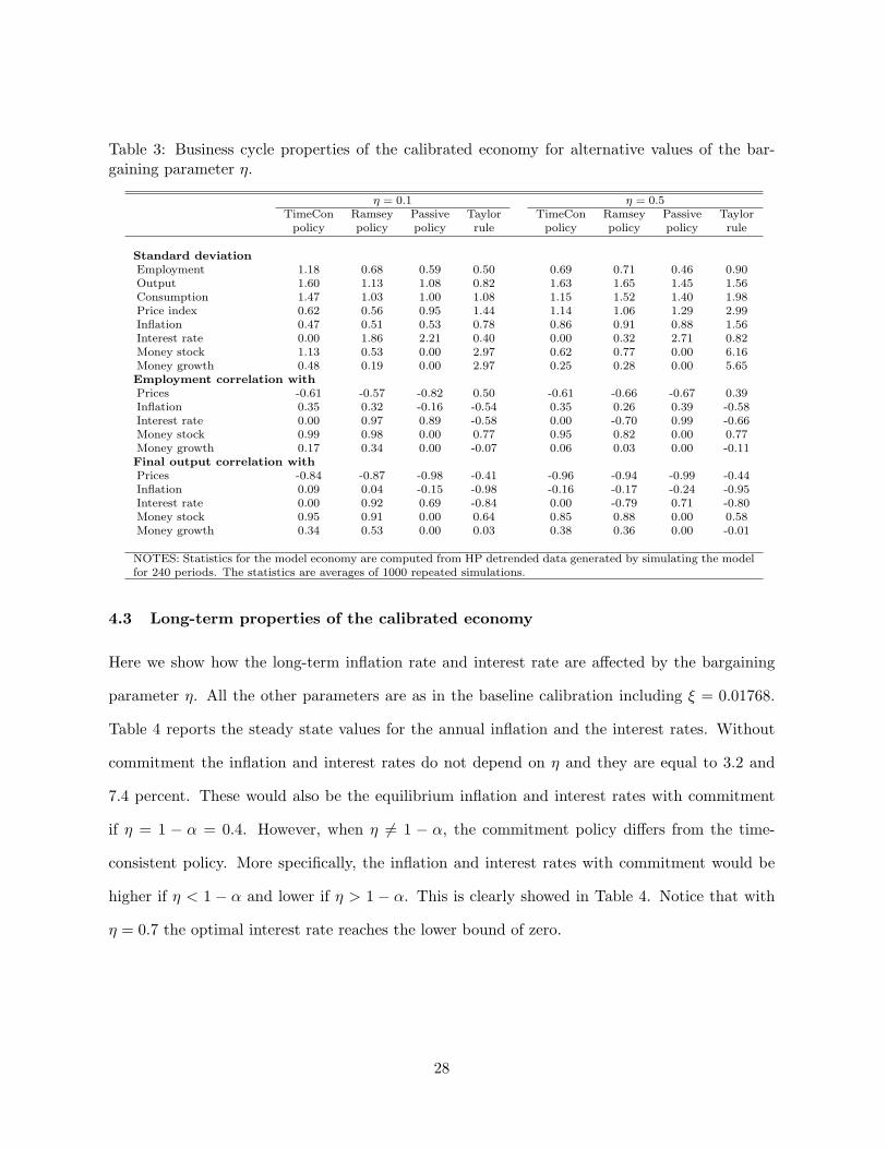
Table 3: Business cycle properties of the calibrated economy for alternative values of the bar-gaining parameter η.

η = 0.1 η = 0.5TimeCon Ramsey Passive Taylor TimeCon Ramsey Passive Taylor

policy policy policy rule policy policy policy rule

Standard deviationEmployment 1.18 0.68 0.59 0.50 0.69 0.71 0.46 0.90Output 1.60 1.13 1.08 0.82 1.63 1.65 1.45 1.56Consumption 1.47 1.03 1.00 1.08 1.15 1.52 1.40 1.98Price index 0.62 0.56 0.95 1.44 1.14 1.06 1.29 2.99Inflation 0.47 0.51 0.53 0.78 0.86 0.91 0.88 1.56Interest rate 0.00 1.86 2.21 0.40 0.00 0.32 2.71 0.82Money stock 1.13 0.53 0.00 2.97 0.62 0.77 0.00 6.16Money growth 0.48 0.19 0.00 2.97 0.25 0.28 0.00 5.65Employment correlation withPrices -0.61 -0.57 -0.82 0.50 -0.61 -0.66 -0.67 0.39Inflation 0.35 0.32 -0.16 -0.54 0.35 0.26 0.39 -0.58Interest rate 0.00 0.97 0.89 -0.58 0.00 -0.70 0.99 -0.66Money stock 0.99 0.98 0.00 0.77 0.95 0.82 0.00 0.77Money growth 0.17 0.34 0.00 -0.07 0.06 0.03 0.00 -0.11Final output correlation withPrices -0.84 -0.87 -0.98 -0.41 -0.96 -0.94 -0.99 -0.44Inflation 0.09 0.04 -0.15 -0.98 -0.16 -0.17 -0.24 -0.95Interest rate 0.00 0.92 0.69 -0.84 0.00 -0.79 0.71 -0.80Money stock 0.95 0.91 0.00 0.64 0.85 0.88 0.00 0.58Money growth 0.34 0.53 0.00 0.03 0.38 0.36 0.00 -0.01

NOTES: Statistics for the model economy are computed from HP detrended data generated by simulating the modelfor 240 periods. The statistics are averages of 1000 repeated simulations.

4.3 Long-term properties of the calibrated economy

Here we show how the long-term inflation rate and interest rate are affected by the bargaining

parameter η. All the other parameters are as in the baseline calibration including ξ = 0.01768.

Table 4 reports the steady state values for the annual inflation and the interest rates. Without

commitment the inflation and interest rates do not depend on η and they are equal to 3.2 and

7.4 percent. These would also be the equilibrium inflation and interest rates with commitment

if η = 1 − α = 0.4. However, when η 6= 1 − α, the commitment policy differs from the time-

consistent policy. More specifically, the inflation and interest rates with commitment would be

higher if η < 1 − α and lower if η > 1 − α. This is clearly showed in Table 4. Notice that with

η = 0.7 the optimal interest rate reaches the lower bound of zero.

28

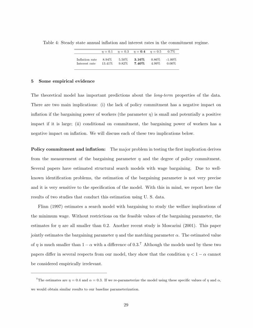
Table 4: Steady state annual inflation and interest rates in the commitment regime.

η = 0.1 η = 0.3 η = 0.4 η = 0.5 0.7%

Inflation rate 8.94% 5.50% 3.16% 0.86% -1.00%Interest rate 13.41% 9.82% 7.40% 4.99% 0.00%

5 Some empirical evidence

The theoretical model has important predictions about the long-term properties of the data.

There are two main implications: (i) the lack of policy commitment has a negative impact on

inflation if the bargaining power of workers (the parameter η) is small and potentially a positive

impact if it is large; (ii) conditional on commitment, the bargaining power of workers has a

negative impact on inflation. We will discuss each of these two implications below.

Policy commitment and inflation: The major problem in testing the first implication derives

from the measurement of the bargaining parameter η and the degree of policy commitment.

Several papers have estimated structural search models with wage bargaining. Due to well-

known identification problems, the estimation of the bargaining parameter is not very precise

and it is very sensitive to the specification of the model. With this in mind, we report here the

results of two studies that conduct this estimation using U. S. data.

Flinn (1997) estimates a search model with bargaining to study the welfare implications of

the minimum wage. Without restrictions on the feasible values of the bargaining parameter, the

estimates for η are all smaller than 0.2. Another recent study is Moscarini (2001). This paper

jointly estimates the bargaining parameter η and the matching parameter α. The estimated value

of η is much smaller than 1−α with a difference of 0.3.7 Although the models used by these two

papers differ in several respects from our model, they show that the condition η < 1− α cannot

be considered empirically irrelevant.

7The estimates are η = 0.4 and α = 0.3. If we re-parameterize the model using these specific values of η and α,

we would obtain similar results to our baseline parameterization.

29

The second problem in testing the importance of policy commitment is to find a proxy for

commitment. One possibility is to assume that countries in which the monetary authority has

greater independence are also countries with a greater ability to commit to future monetary

policies. Several studies have investigated the importance of Central Bank Independence for

explaining inflation but they reach contrasting results depending on the set of countries used

in the empirical investigation. For the restricted group of high-income countries, Central Bank

Independence seems to reduce inflation (see Grilli, Masciandaro, & Tabellini (1991)), but for

developing countries the impact is estimated to be positive, although not always statistically

significant (see Cukierman, Webb, & Neyapti (1992) and Campillo & Miron (1997)).

These results are consistent with the predictions of our theoretical model in the following sense.

According to our proxy variable for the parameter η (which we will describe below), the bargaining

power of workers is on average greater in high income countries than in countries with middle and

low levels of income. This is clearly shown in Table F in the Appendix. Therefore, the condition

η > 1 − α is more likely to be satisfied in high income countries while the condition η < 1 − α

is more likely to be satisfied in middle and low income countries.8 Under this interpretation

our theory predicts that the inflation impact of Central Bank Independence is negative in high

income countries and positive in middle and low income countries. This seems consistent with the

findings of the previous empirical literature as discussed above. Although this is not a rigorous

testing of our theory, the empirical evidence is consistent with it.

Bargaining power and inflation: If we think that policy makers are subject to some form of

commitment, then countries in which employers have greater bargaining power should experience

8The evidence of a small value of η for the United States is not inconsistent with this view. In fact, the

bargaining power of workers in the Unites States is considered to be one of the lowest among industrialized

countries. Consequently, the condition η > 1−α may still dominate for the whole group of industrialized countries

even if it does not hold for the United States. From Table F we can verify that the proxy variable for the bargaining

power of employers in the United States is one of the highest among the high income countries.

30

higher inflation. In this section we provide some evidence in support of this result. Before

discussing the empirical evidence, however, we should justify the assumption of commitment.

Although the previous analysis focused on the extreme cases of full discretion and full com-

mitment, the result that the bargaining power of workers affects the equilibrium inflation rate

requires only a weak form of commitment. More specifically, this result also holds if the growth

rate of money is chosen two periods in advance (two-period commitment). In fact, according to

the analysis of Section 3, the profitability of a new job does not depend on the current inflation

rate but on the inflation rate two periods from now (see equation (28)). This pre-commitment

of policy could be the result of a lag between the moment in which the policy maker chooses the

policy instruments, and the moment in which these instruments affect the real economy. When

we adopt this interpretation of policy commitment, the assumption that countries “commit” to

future policies is not unreasonable. Notice that the same result would be reached if the policy

maker chooses the nominal interest rate instead of the growth rate of money. In this case a

one-period commitment would be sufficient.

To capture the cross-country differences in the bargaining power of employers and workers,

we use the ratio of the value added generated in the manufacturing sector to the wages paid in

that sector. The idea underlying the use of this proxy variable is that greater bargaining power

of employers should allow them to appropriate a larger share of the surplus, where the surplus

is approximated with value added. Higher values of this ratio are then interpreted as higher

bargaining power of employers (and lower bargaining power of workers). We use data published

by the United Nation Industrial Development Organization (UNIDO) for the years 1990 through

2000 for a large set of countries. The set of countries and years available for each country are

reported in Appendix F.

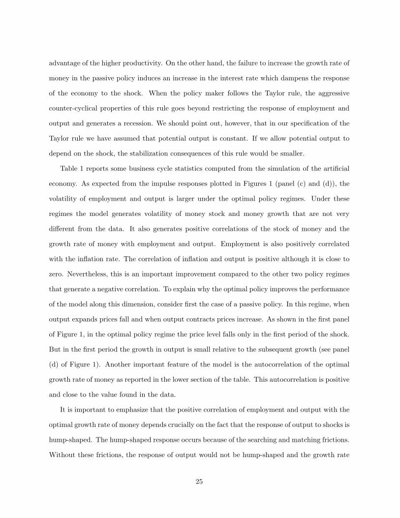
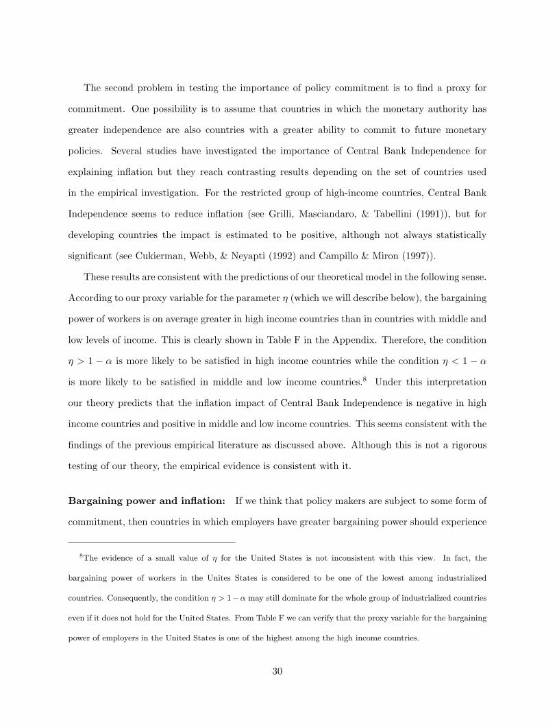
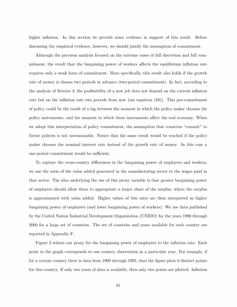
Figure 2 relates our proxy for the bargaining power of employers to the inflation rate. Each

point in the graph corresponds to one country observation in a particular year. For example, if

for a certain country there is data from 1990 through 1995, then the figure plots 6 distinct points

for this country. If only two years of data is available, then only two points are plotted. Inflation

31

rates are based on the GDP deflator published by the World Bank in the World Development

Indicators. The inflation rates are for the same year of the proxy variable.

y = 1.5178x + 3.0453R2 = 0.1127

-10

-5

0

5

10

15

20

25

30

35

0 1 2 3 4 5 6 7 8 9 10 11 12 13

Bargaining proxy

Infla

tion

rate

Figure 2: Cross-country correlation of inflation with the bargaining proxy.

Figure 2 shows that there is a positive association between our bargaining power proxy and

the inflation rate. The correlation coefficient is 0.34. A similar correlation coefficient is obtained

if we average the variables for each country over the years of available data (so that countries

with a smaller number of observations do not get lower weights). In constructing the graph we

have excluded countries for which the inflation rates are above 30 percent. The reason is that

situations of hyperinflation cannot be rationalized as the outcome of optimal monetary policies.

However, the sign of the correlation is not affected by this upper bound.

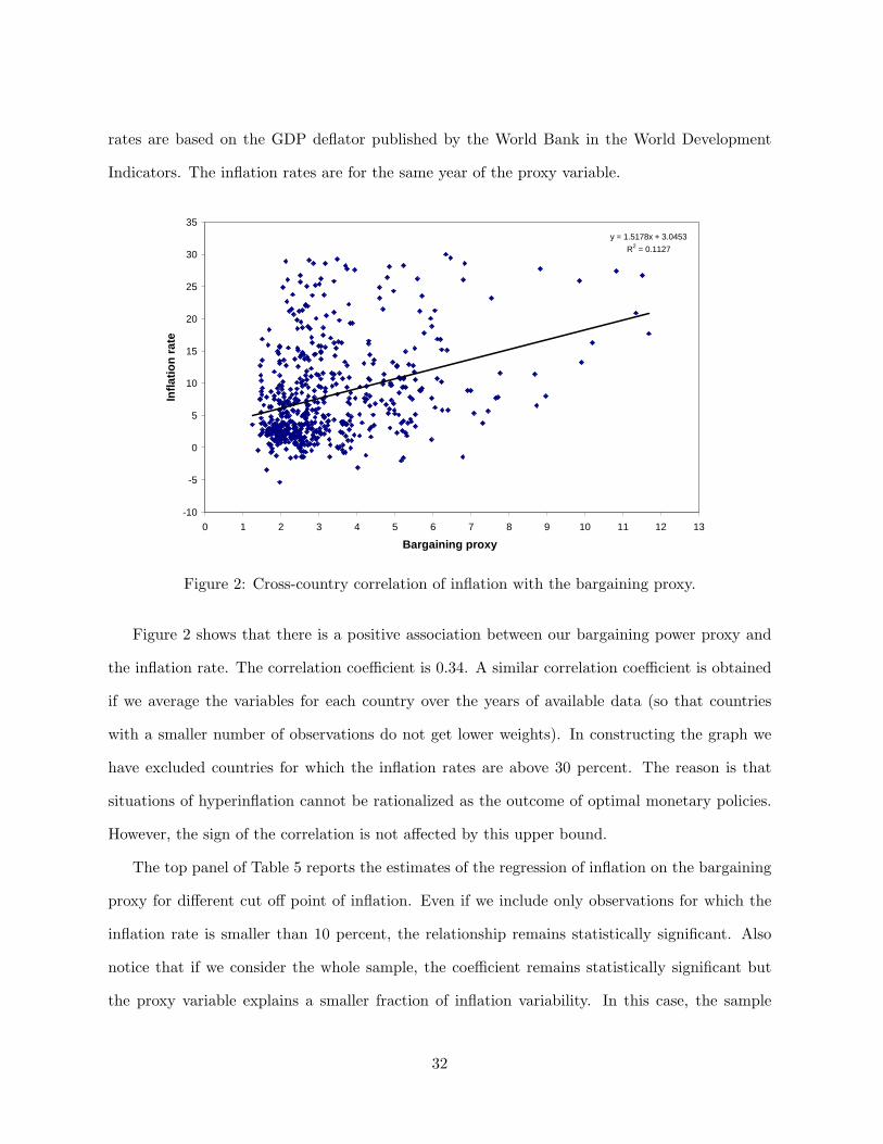
The top panel of Table 5 reports the estimates of the regression of inflation on the bargaining

proxy for different cut off point of inflation. Even if we include only observations for which the

inflation rate is smaller than 10 percent, the relationship remains statistically significant. Also

notice that if we consider the whole sample, the coefficient remains statistically significant but

the proxy variable explains a smaller fraction of inflation variability. In this case, the sample

32

includes countries with inflation rates that are above 1,000 percent like in the case of some Latin

American countries in the early 90s.

Table 5: Linear regression of inflation on the bargaining proxy.

Whole Inflation Inflation Inflationsample <50% <30% <10%

Intercept -6.05 4.57∗ 4.15∗ 2.44∗

(21.8) (0.75) (0.57) (0.34)Bargaining proxy 14.69∗ 1.50∗ 1.15∗ 0.51∗

(5.08) (0.19) (0.15) (0.10)

# Obs. 672 606 573 403R-square 0.012 0.093 0.096 0.056

Whole Inflation Inflation Inflationsample <50% <30% <10%

Intercept -6.41 9.52∗ 8.28∗ 4.40∗

(27.55) (0.88) (0.66) (0.40)Bargaining proxy 14.71∗ 1.22∗ 0.91∗ 0.34∗

(5.12) (0.18) (0.14) (0.10)Productivity/10000 0.13 -1.60∗ -1.30∗ -0.48∗

(6.00) (0.17) (0.13) (0.06)

# Obs. 672 606 573 403R-square 0.012 0.206 0.236 0.185

Note: ∗ Significant at 1% level.

The positive correlation between the inflation rate and our bargaining proxy may be the

result of the fact that developing countries have lower fractions of value added paid in the form

of wages and these countries experience on average higher inflation rates. To capture the impact

of the country development, we extend our regression equation by including a proxy for the level

of development. This variable is given by the average productivity in the manufacturing sector

computed by dividing the value added by the number of workers employed in this sector. To

avoid endogeneity problems, the productivity variable is for the year preceding the first year of

available data for inflation. The bottom panel of Table 5 shows that the bargaining proxy remains

statistically significant. This result is robust to the use of per-capita GDP as a proxy for the level

of development instead of manufacturing productivity.

33

6 Conclusion

In this paper we have analyzed the properties of the optimal monetary policy in a world where

inflationary monetary interventions have expansionary effects in the economy through the liq-

uidity channel. We find that if technology shocks are the main driving force of business cycle

fluctuations, then the optimal monetary policy is pro-cyclical and amplifies the response of the

economy to these shocks. The optimality of a pro-cyclical policy derives from the assumption

that technology shocks are the main source of business cycle fluctuations. Different conclusions

may be reached if we consider alternative sources of fluctuations.

We have also analyzed the long-run properties of the optimal and time-consistent policy and

compared it to the long-term properties of the optimal policy under commitment. The main

finding is that the ability to commit could lead to higher inflation if certain conditions pertaining

to the structure of the labor market are satisfied. More specifically, higher inflation would be

optimal if the employers’ share of the surplus is too large. In this case higher inflation and

interest rates are optimal because they reduce the surplus generated by a match, and therefore,

the excessive creation of jobs. This result requires only a weak version of commitment. For

example, this would be the outcome if the policy maker chooses the policy instruments two

periods in advance (two-period commitment). This weak form of commitment could derive from

formal and informal institutional restrictions to the discretion of the policy maker, as well as

from the lags through which the policy instruments impact on the real sector of the economy. In

this sense, the assumption of commitment is not unreasonable and there is some cross-country

evidence supporting our result. In particular, countries in which the fraction of value added paid

in the form of wages (proxing for the bargaining power of workers) is lower, are also the countries

that tend to experience higher inflation.

We conclude by pointing out that there could be other mechanisms that make the Friedman

rule suboptimal. One of this mechanism derives from the distributional effects of inflation which

are ignored in this paper. This mechanism is studied in Albanesi (2002).

34

A Proof of lemma 3.1

If the cash-in-advance constraint is binding, the aggregate version of the budget constraint (16) can be written as

(1+g) = (D+g)(1+R)+(1−ν)PNAXν where the last term is simply the aggregate value of wages and profits paid

by firms. Remember that the wage and profit paid by an individual firm is (1 − ν)AXν .9 Combining the budget

constraint with the equilibrium in the loans market D+g = PXN and rearranging, we get R = ν(1+g)/(D+g)−1.

This relation is valid as long as ν(1 + g)/(D + g)− 1 ≥ 0. Otherwise the cash-in-advance constraint is not binding

and the interest rate cannot be smaller than zero. Q.E.D.

B Proof of proposition 3.1

Consider the following planner’s problem in the choice of the input X and the number of vacancies V :

Ω(A, N) = maxX,V

C − aN + β E Ω(A′, N ′)

(30)

subject to

C = N(AXν −X)− V κ (31)

N ′ = (1− λ)N + m(V, 1−N) (32)

Equation (31) defines consumption from the aggregate resource constraint and (32) is the law of motion for

the next period employment. The first order conditions are:

−κ + βm1E

[A′(X ′)ν −X ′ − a +

κ

m′1

(1− λ−m′2)

]= 0 (33)

X = (νA)1

1−ν (34)

where m1 and m2 are the derivatives of the matching function with respect to the first and second arguments.

Now consider the household problem specified in (14). The first order conditions are:

κ

q= β E

(βP ′π′

P ′′(1 + g′)

)+ β E

((1− λ)κ

q′

)(35)

−E(

1

P ′

)+ βE

((1 + R′)

P ′′(1 + g′)

)= 0 (36)

These conditions must be satisfied in the competitive equilibrium. Using equation (11) to eliminate π′, condition

9All variables are denoted in capital letters because they are aggregate variables.

35

(35) can be written as:

−κ + β(1− η)qE

[(A′(X ′)ν −X ′(1 + R′)

)E

(βP ′

P ′′(1 + g′)

)− a +

κ

(1− η)q′(1− λ− ηh′)

]= 0 (37)

Because in the competitive equilibrium X = (νA/(1+R))1

1−ν (see proposition 1.1), equation (34) implies that

the optimal interest rate for the planner is zero. With R = 0, equation (37) is not necessarily equal to (33), that is,

the optimal number of new vacancies may not be optimal. However, equation (37) does not depend on the current

interest rate, but only on the future interest rate. The planner will be able to affect the rate of vacancy creation

only if it can credibly commit to R′ today. Without commitment the value of R′ chosen today will not be optimal

tomorrow. Consequently, the zero interest rate policy is the optimal and time-consistent policy. However, the

optimal policy in terms of the growth rate of money is not necessarily unique because at R = 0 the cash-in-advance

constraint is not binding. To show that the zero interest rate policy is unique, it is enough to show that the

policy maker will always deviate from a policy rule that do not implement R = 0. Let Ψ be the policy rule that

determined the future growth rates of money and let g be the current growth rate of money determined by this

policy, that is, g = Ψ(s). Given (g, Ψ), the equilibrium condition implies either R = 0 or R > 0 (the interest rate

cannot be negative). In the first case the planner does not need to change g to obtain R = 0. If instead R > 0,

then it will change g to obtain R = 0. This is because a change in the current growth rate of money will not affect

the next period states (in particular employment). Therefore, the planner will deviate from any policy that allows

for a positive nominal interest rate. Q.E.D.

C Proof of proposition 3.2

Using the equilibrium condition in the loans market D + g = PXN to eliminate the term D + g in the aggregate

budget constraint, we get 1 + g = PN [X(1 + R) + (1 − ν)AXν ]. Because X(1 + R) + (1 − ν)AXν = AXν , this

equation can be written as 1 + g = PY where Y = NAXν is aggregate gross output. This condition must be

satisfied in each period. Therefore, it must also be satisfied in the next two periods, that is, P ′Y ′ = 1 + g′ and

P ′′Y ′′ = 1 + g′′. Using these two conditions we can derive:

E

(Y ′′

Y ′(1 + g′′)

1

P ′

)= E

(1

P ′′(1 + g′)

)(38)

Assume that the optimal policy is gt = βEt−1Yt/Yt−1 − 1. To verify that this policy implements a zero nominal

interest rate, substitute this policy in equation (38). This gives:

E(

1

P ′

)= βE

(1

P ′′(1 + g′)

)(39)

36

From the household’s first order conditions, equation (36), we observe that this condition implies a zero nominal

interest rate. Therefore, the policy gt = βEt−1Yt/Yt−1 − 1 is optimal and time-consistent. We want to show

now that this policy is unique. Notice that any policy that implements a zero nominal interest rate must satisfies

condition (39). Then given a policy that satisfies this condition, the next period stock of deposits is determined

and it cannot be changed in the next period. If the optimal policy rule is different from gt = βEt−1Yt/Yt−1 − 1,

it must have some stochastic component that is unpredictable so that condition (39) is still satisfied. But then

ex-post, this stochastic component may induce an interest rate different from zero and the policy maker will deviate

from this policy. Therefore, this stochastic component cannot be part of the optimal policy. Moreover, because

the growth rate of final output N(AXν −X) is equal to the growth rate of gross output Y = NAxν when R = 0,

then g = βE−1(1 + gY )− 1. Q.E.D.

D Proof of proposition 3.3

Consider the planner problem (30) with first order conditions (33) and (34). The first order conditions for the

household in the competitive equilibrium are given by (36) and (37). If η = 1−α, R = 0 and E′[βP ′/(P ′′(1+g′))] =

1, it can be verified that (37) is exactly equal to (33). This is because m1 = (1 − η)q and m2 = ηh. This policy

can be implemented by setting the growth rate of money as follows:

1 + gt+1 =βPt

1 + gtEtYt+1 (40)

where Yt+1 = At+1Xνt+1 is gross output under the assumption that Rt = 0 and Et[βPt/(Pt+1(1 + gt))] = 1 for all

t = 0, 1, ... Notice that the growth rate of money does not depend on the current shock but only on the shocks up

to the previous period.

We can verify that policy (40) implements Rt = 0 and E[βPt/(Pt+1(1+gt))] = 1. Because 1+gt+1 = Pt+1Yt+1

(see proof of proposition 3.2), after rearranging and taking expectations we get Et(1+gt+1/Pt+1) = EtYt+1. Using

this equation to eliminate EYt+1 in (40) we obtain Et[βPt/(Pt+1(1+gt))] = 1. This condition also holds one period

forward. Therefore, 1/Pt+1 = Et+1[β1/(Pt+2(1 + gt+1))]. Taking the expectation at time t we have:

Et

(1

Pt+1

)= βEt

(1

Pt+2(1 + gt+1)

)(41)

Comparing this equation with condition (36) we verify that policy (40) delivers a zero nominal interest rate and

reaches the first best.

Now consider the case η < 1− α and assume that the policy maker follows the same policy (40). As we have

seen above this policy delivers a zero interest rate. Comparing (33) with (37) we can see that this policy induces

a number of vacancies which is smaller than the social optimum. To see this, let’s first observe that under policy

37

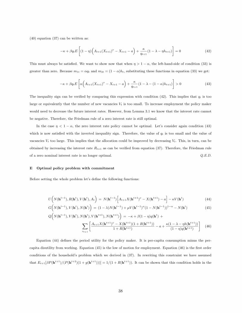
(40) equation (37) can be written as:

−κ + βqtE

[(1− η)

(At+1(Xt+1)

ν −Xt+1 − a)

+κ

qt+1(1− λ− ηht+1)

]= 0 (42)

This must always be satisfied. We want to show now that when η > 1 − α, the left-hand-side of condition (33) is

greater than zero. Because m1t = αqt and m2t = (1− α)ht, substituting these functions in equation (33) we get:

−κ + βqtE

[α(At+1(Xt+1)

ν −Xt+1 − a)

+κ

qt+1(1− λ− (1− α)ht+1)

]> 0 (43)

The inequality sign can be verified by comparing this expression with condition (42). This implies that qt is too

large or equivalently that the number of new vacancies Vt is too small. To increase employment the policy maker

would need to decrease the future interest rates. However, from Lemma 3.1 we know that the interest rate cannot

be negative. Therefore, the Friedman rule of a zero interest rate is still optimal.

In the case η < 1 − α, the zero interest rate policy cannot be optimal. Let’s consider again condition (43)

which is now satisfied with the inverted inequality sign. Therefore, the value of qt is too small and the value of

vacancies Vt too large. This implies that the allocation could be improved by decreasing Vt. This, in turn, can be

obtained by increasing the interest rate Rt+1 as can be verified from equation (37). Therefore, the Friedman rule

of a zero nominal interest rate is no longer optimal. Q.E.D.

E Optimal policy problem with commitment

Before setting the whole problem let’s define the following functions:

U(N(ht−1), R(ht), V (ht), At

)= N(ht−1)

[At+1X(ht+1)ν −X(ht+1)− a

]− κV (ht) (44)

G(N(ht−1), V (ht), N(ht)

)= (1− λ)N(ht−1) + µV (ht−1)α(1−N(ht−1))1−α −N(ht) (45)

Q(N(ht−1), V (ht), N(ht), V (ht+1), N(ht+1)

)= −κ + β(1− η)q(ht) +∑

zt+1

[At+1X(ht+1)ν −X(ht+1)(1 + R(ht+1))

1 + R(ht+1)− a +

κ(1− λ− ηh(ht+1))

(1− η)q(ht+1)

](46)

Equation (44) defines the period utility for the policy maker. It is per-capita consumption minus the per-

capita disutility from working. Equation (45) is the low of motion for employment. Equation (46) is the first order

conditions of the household’s problem which we derived in (37). In rewriting this constraint we have assumed

that Et+1[βP (ht+1)/(P (ht+2)(1 + g(ht+1)))] = 1/(1 + R(ht+1)). It can be shown that this condition holds in the

38

optimal policy.10 This implies that the first order condition (36) in the household’s problem is satisfied. Using

these functions the Ramsey problem can be written as:

maxN(ht),R(ht),V (ht)∞

t=0

∞∑t=0

βt∑

ht∈Ht

p(ht)

[U

(N(ht−1), R(ht), V (ht), At

)](47)

subject to

G(N(ht−1), V (ht), N(ht)

)= 0 (48)

Q(N(ht−1), V (ht), N(ht), V (ht+1), N(ht+1)

)= 0 (49)

with N(h−1) given. In this problem the policy maker chooses the sequence of interest rates, vacancies and em-

ployment. The numerical solution of this problem is obtained by linearizing the first order conditions around the

steady state.

10To see this result, it is sufficient to show that the interest rate at time t depends only on the history up to

time t− 1 (it does not depend on the current shock). This can be seen by looking at condition (37). Once we have

established that the interest rate does not depend on the current shock (but only on the previous shocks), we can

show that Et+1[βP (ht+1)/(P (ht+2)(1 + g(ht+1)))] = 1/(1 + R(ht+1)) following the same argument of the proof of

proposition 3.3.

39

F Data set for the analysis of Section 5

Bargaining Inflation Bargaining InflationCountry proxy rate Country proxy rate

Albania (1990) 2.8 -0.5 Jordan (1990-1997) 4.2 4.9Algeria (1990-1996) 2.6 28.7 Kenia (1990-1999) 2.8 13.6Argentina (1990, 1993-1996) 2.9 416.2 Korea (1990-2000) 4.3 5.4Australia (1990-1992) 2.5 2.3 Luxembourg (1990-1994) 1.8 3.1Austria (1990-2000) 1.9 2.2 Macau (1990-1997) 1.8 7.2Bahamas (1990-1991) 2.1 2.2 Malawi (1990-1998) 3.3 29.1Bangladesh (1990-1992, 1995, 1997) 3.5 5.5 Malaysia (1990-2000) 3.7 3.8Barbados (1990-1997) 2.6 3.0 Malta (1990-1996) 2.0 3.1Belgium (1990-1992) 2.4 3.1 Mauritius (1990-1997) 2.3 6.9Bolivia (1990-1997) 9.2 11.3 Mexico (1990-2000) 5.1 19.2Botswana (1990-1995) 2.3 8.9 Mongolia (1990-1995) 4.3 107.8Brazil (1990,1992-1995) 5.0 1558.3 Moldova (1993-1995) 6.8 391.9Bulgaria (1991-1996) 3.0 99.0 Marocco (1990-1999) 2.7 3.3Burundi (1990-1991) 5.0 5.0 Namibia (1994) 3.0 15.7Cameroon (1990-1999) 2.8 4.2 Nepal (1990-1994, 1996) 4.6 9.1Canada (1990-2000) 2.4 1.7 Netherlands (1990-2000) 2.0 2.1Central African Republic (1990-1993) 2.0 -0.1 New Zealand (1990-1996) 1.9 1.8Sri Lanka (1990-1998) 5.3 10.9 Nigeria (1991-1996) 17.1 46.2Chile (1990-2000) 5.4 9.3 Norway (1990-1999) 1.7 2.4Colombia (1990-2000) 6.0 21.5 Pakistan (1990-1991, 1996) 4.5 9.3Costa Rica (1990-1999) 2.9 20.8 Panama (1990-1999) 2.6 2.0Croatia (1990-1992) 4.2 264.7 Paraguay (1991) 4.6 24.8Cyprus (1990-2000) 2.1 3.7 Peru (1990-1996) 6.0 1222.6Denmark (1990-1991) 1.6 3.2 Philippines (1990-1997) 5.0 9.46Ecuador (1990-1999) 6.9 39.1 Poland (1990-2000) 3.2 28.0El Salvador (1993-1998) 3.2 8.0 Romania (1990-1993) 2.7 159.0Ethiopia (1990-1996) 4.8 7.9 Russia (1993-1998) 3.2 238.9Fiji (1990-1992) 2.1 5.5 Senegal (1990-1997) 2.8 4.6Finland (1990-1999) 2.2 2.2 Sierra Leone (1993) 11.5 26.7France (1990-1992) 1.7 2.6 Singapore (1990-2000) 3.3 1.6Gabon (1991-1995) 1.7 7.3 Slovakia (1993-1994) 2.6 17.9Gambia (1993) 5.5 5.1 Slovenia (1990-1999) 1.8 71.7Ghana (1993-1995) 6.1 35.0 South Africa (1990-2000) 2.0 10.4Greece (1990-2000) 2.6 10.6 Zimbabwe (1990-1999) 3.5 25.3Honduras (1990-1995) 2.1 20.6 Spain (1990-1995, 1990-2000) 2.2 5.1Hong Kong (1990-1999) 1.9 5.1 Suriname (1990-1993) 3.7 43.9Hungary (1990-2000) 2.4 19.9 Swaziland (1990-1995) 3.5 13.3Iceland (1990-1996) 1.5 5.3 Sweden (1990-2000) 2.3 2.8India (1990-2000) 3.0 8.2 Syria (1990-1998) 4.5 8.3Indonesia (1990-1999) 6.6 16.4 Thailand (1990-1994) 7.7 5.0Iran (1990-1993) 2.8 26.3 Trinidad and Tobago (1990-1995) 2.7 8.1Ireland (1990-1999) 4.8 3.0 Tunisia (1993-1999) 2.8 4.3Israel (1990-1996) 1.5 13.0 Turkey (1990-2000) 4.7 71.3Italy (1990-2000) 2.0 4.3 Egypt (1990-1997) 3.0 11.7Cote d’Ivoire (1994-1995, 1997) 2.7 19.1 United Kingdom (1990-1995) 2.2 4.2Jamaica (1990-1996) 2.9 36.4 Unites States (1990-1995) 2.9 2.8Japan (1990-2000) 3.1 0.5 Uruguay (1990-1999) 4.2 45.4

Venezuela (1990-1998) 9.1 45.8

Source: UNIDO Industrial Statistics and World Bank Development Indicators

40

References

Albanesi, S., Chari, V. V., & Christiano, L. J. (1999). A positive theory of monetary policy in

a natural rate model. Unpublished manuscript, Department of Economics, Northwestern

University.

Albanesi, S. (2002). The time consistency of optimal monetary policy with heterogeneous agents.

Unpublished manuscript, Bocconi University.

Andolfatto, D. (1996). Business cycles and labor-market search. American Economic Review,

86 (1), 112–32.

Barro, R. J. & Gordon, D. B. (1983). A positive theory of monetary policy in a natural rate

model. Journal of Political Economy, 91 (4), 589–610.

Barth, M. J. & Ramey, V. A. (2001). The cost channel of monetary transmission. In Bernanke,

B. S. & Rogoff, K. (Eds.), NBER Macroeconomics Annual, pp. 199–239. MIT Press, Cam-

bridge, Massachusetts.

Blanchard, O. & Diamond, P. (1989). The beveridge curve. Brookings Papers on Economic

Activity, 89 (1), 1–76.

Campillo, M. & Miron, J. A. (1997). Why does inflation differ across countries?. In Romer,

C. D. & Romer, D. H. (Eds.), Reducing Inflation: Motivationand Strategy, pp. 379–418.

The University of Chicago Press, Chicago.

Chari, V. V., Christiano, L. J., & Kehoe, P. J. (1996). Optimality of the friedman rule in

economies with distorting taxes. Journal of Monetary Economics, 37 (2), 203–223.

Christiano, L. J. & Eichenbaum, M. (1995). Liquidity effects, monetary policy, and the business

cycle. Journal of Money Credit and Banking, 27 (4), 1113–36.

Christiano, L. J., Eichenbaum, M., & Evans, C. L. (1996). The effects of monetary policy shocks:

evidence from the flow of funds. Review of Economics and Statistics, 78 (1), 16–34.

41

Cooley, T. F. & Hansen, G. D. (1995). Money and the business cycle. In Cooley, T. F. (Ed.),

Frontiers of Business Cycle Research, chap. 7. Princeton University Press, Princeton, New

Jersey.

Cooley, T. F. & Quadrini, V. (1999). A neoclassical model of the phillips curve relation. Journal

of Monetary Economics, 44 (2), 165–93.

Cukierman, A., Webb, S. B., & Neyapti, B. (1992). Measuring the independence of central bank

and its effect on policy outcome. World Bank Economic Review, 6 (3), 353–98.

Den-Haan, W. J., Ramey, G., & Watson, J. (2000). Job destruction and the propagation of

shocks. American Economic Review, 90 (3), 482–98.

Flinn, C. J. (1997). Minimum wage effects on labor market outcomes under search with bargain-

ing. Unpublished manuscript, New York University.

Fuerst, T. S. (1992). Liquidity, loanable funds, and real activity. Journal of Monetary Economics,

29 (4), 3–24.

Grilli, V., Masciandaro, D., & Tabellini, G. (1991). Political and monetary institutions and public

financed policies in the industrial countries. Economic Policy, 13, 341–92.

Hamilton, J. D. (1997). Measuring the liquidity effect. American Economic Review, 87 (1), 80–97.

Hosios, A. J. (1990). On the efficiency of matching and related models of search unemployment.

Review of Economic Studies, 57 (2), 279–298.

Ireland, P. N. (1996). The role of countercyclical monetary policy. Journal of Political Economy,

104 (4), 704–23.

Kydland, F. & Prescott, E. C. (1977). Rules rather than discretion: the inconsistency of optimal

plans. Journal of Political Economy, 85 (3), 473–491.

Leeper, E. M., Sims, C. A., & Zha, T. (1996). What does monetary policy do?. Brookings Papers

on Economic Activity, 96 (2), 1–63.

42

Lucas, R. E. (1990). Liquidity and interest rates. Journal of Economic Theory, 50 (2), 273–64.

Merz, M. (1995). Search in the labor market and the real business cycle. Journal of Monetary

Economics, 36, 269–300.

Mortensen, D. T. & Pissarides, C. A. (1994). Job creation and job destruction in the theory of

unemployment. Review of Economic Studies, 61, 397–415.

Moscarini, G. (2001). Skill and luck in the thory of turnover. Unpublished manuscript, Yale

University.

Pissarides, C. (1988). The search equilibrium approach to fluctuations in employment. American

Economic Review, 78 (2), 363–68.

Sargent, T. J. (1998). The Conquest of American Inflation. Princeton University Press, Princeton,

New Jersey.

Shi, S. (1998). Search for a monetary propagation mechanism. Journal of Economic Theory,

81 (2), 314–352.

Taylor, J. B. (1998). An historical analysis of the monetary policy rules. NBER Working Paper

Series, # 6768.

43