Optimal Monetary Policy, InternationalCoordination, and Currency Unions

Lucas Herrenbrueck

University of California, Davis

Version of October 6, 2012

PRELIMINARY AND INCOMPLETE

Abstract

What is the optimal inflation rate in an open economy, and when are currency

unions a good idea? I investigate these questions using a monetary open economy

model where firms have market power because of search frictions. Consumers re-

spond to inflation by increasing their search effort, and as a result, inflation has non-

monotonic effects in steady state. The optimal inflation rate depends on the fun-

damendals of the economy, such as the disutility of search or the cost of firm entry,

and on the inflation rates of trading partners. When countries coordinate their mone-

tary policies, inflation will be lower and welfare will be higher than in non-cooperative

equilibrium. However, coordinating policy is not the same as conducting the same pol-

icy. For countries with different fundamentals, there may be welfare losses from join-

ing a currency union. The joint welfare loss would be small but the welfare effects on

individual countries are asymmetric and can be severe. Preliminary analysis suggests

that the model can account for some features of the macroecomic divergence of the

Eurozone in the 1990s and 2000s.

1

1 Introduction

What is the optimal monetary policy in an open economy? Extensive research has ad-dressed the question of how monetary policy should respond to temporary shocks, do-mestic or foreign, but has ignored the effects of structural factors on the optimal long-runmoney growth rate, and therefore the optimal long-run inflation rate. Models of such ef-fects exist, but have previously been limited to closed economies. However, the questionof optimal money growth may be especially relevant in an international context. First,there may be benefits from coordinating long-run inflation rates between countries. Sec-ond, there may be costs to giving up an independent choice of the money growth rate,such as when pegging the exchange rate or forming a currency union.

In order to address these questions, I use a model of a monetary economy with searchfrictions and endogenous search effort. Specifically, I build on the optimal inflation modelof Head and Kumar (2005), which studies the endogenous choice of search effort by con-sumers in a monetary-search model with price posting. I extend this model in three di-rections: ex-ante firm heterogeneity, free entry of firms, and international trade amongan arbitrary number of countries. International trade provides a channel through whichmonetary policy in one country affects another. Firm heterogeneity and free entry allowme to link the results of the model with the recent experience of the Eurozone.

In a closed-economy version of the model, the results are similar to those of Head andKumar (2005). The optimal long-run inflation rate is robustly above the Friedman rule(deflation at the rate of time preference), for the following reason: inflation acts as a taxon real balances, but for low levels of inflation, other channels can outweigh this negativeeffect. The principal channel through which inflation has positive effects is the choice ofsearch effort by consumers. Search effort limits market power in the aggregate, but indi-vidual consumers do not take this externality into account. By increasing price dispersion,inflation stimulates search effort, which reduces market power and enhances welfare. Thiseffect dominates for low levels of inflation, but not for high ones. As a result, the inflationrate which maximizes welfare is positive. Extending the original results, I characterizehow this optimal rate of inflation depends on structural parameters. Most notably, it is anincreasing function of the disutility of search effort, and of the cost of firm entry.

Next, I solve a two-country version of the model. Firms can sell at home or abroad, butthey are subject to iceberg trade costs and to local-currency pricing. I find that inflationis a beggar-thy-neighbor policy for two reasons: first, some of the inflation tax is passedon to foreign consumers; second, inflation increases search effort at home, which limits

2

the market power of foreign firms. Consequently, when trading partners cooperate tochoose jointly optimal inflation rates, inflation will be lower and welfare will be higherthan in non-cooperative equilibrium. Choosing the same inflation rate, however, cannotbe optimal when countries have structural differences, such as in the disutility of searcheffort or the cost of firm entry. This implies that currency unions exert a welfare cost,but the effects are necessarily asymmetric. As a benchmark case, assume that prospectivemembers of a currency union are coordinating their inflation rates optimally. If they agreeto a common inflation rate that is optimal for the union as a whole, then countries whoinitially had lower inflation will gain, while countries who initially had higher inflationwill lose.

These results add to our understanding of optimum currency areas. Starting with Mundell(1961), the theory has focused largely on the adjustment of the economy to temporaryshocks, and on how currency unions can affect this adjustment. Similarly, papers study-ing optimal monetary policy in an open economy typically model an environment wherethe only role of monetary policy is to respond to fluctuations. For example, Corsetti andPesenti (2009) find that under local currency pricing, any type of increase in the moneygrowth rate is a beggar-thy-neighbor policy, but with transitory effects. In the presentpaper, on the other hand, unexpected increases have no effects at all, but permanent in-creases have permanent effects.

Such permanent effects of changes in long-run money growth rates are common to monet-ary-search models with endogenous search effort. The debt to Head and Kumar (2005) hasalready been acknowledged. In an early contribution, Li (1995) introduced the “hot potatoeffect”, where inflation increases the frequency of trading. Wright, Liu, and Wang (2009)study the effect further, but in contrast to the present paper, they find that search effort de-creases with inflation and only participation increases. The externality due to endogenoussearch effort (or entry) is studied by Shi (2006), Berentsen, Rocheteau, and Shi (2007), andCraig and Rocheteau (2008). In these papers, the externality of endogenous search couldbe positive or negative; this arises from the bargaining mechanism that determines theterms of trade in their models. In my paper, on the other hand, the terms of trade aredetermined by price posting, and the externality of search effort is always positive: moresearch effort puts pressure on firms to reduce markups, but individual buyers do not takethis into account.

So far, the monetary-search literature has mostly focused on environments with homoge-neous firms or sellers. However, firm heterogeneity is important for the following reason.Higher search effort always shifts production to the cheaper firms, and when firms are

3

heterogeneous, there is a direct welfare gain because the cheaper firms are more efficient.Two consequences are apparent. First, in models of a single homogeneous good, pricedispersion is associated with a welfare loss, and is one of the reasons for the welfare costof inflation.1 This is not true in the present paper, because prices should reflect costs, andlow price dispersion indicates that the efficient firms charge high markups. Second, totalfactor productivity is affected by search effort, and hence by monetary policy.

The premise of my paper is that inflation affects the real economy through price disper-sion, to which consumers respond by choosing their search effort (Head and Kumar, 2005).Recently, this premise has received some empirical support. Caglayan, Filiztekin, andRauh (2008) find that price dispersion is V-shaped as a function of inflation and that theamount of dispersion is related to search costs. Using European Union price data, Beckerand Nautz (2010) and Becker (2011) find this V-shaped relationship disappears in highlyintegrated markets, where search costs are presumably low.

To my knowledge, the conclusion that very low rates of inflation are associated with re-ductions in output, first proposed by Head and Kumar (2005) and supported in my model,has not received direct empirical attention in the existing literature. However, it is cer-tainly consistent with the literature on persistent large output gaps (surveyed by Meier,2010). Consider for example Meier’s observation that “disinflation has tended to taperoff at very low positive inflation rates, arguably reflecting downward nominal rigiditiesand well-anchored inflation expectations”, which is also consistent with a model in whichexpectations of slower money growth initially bring on disinflation, but then cause out-put to fall and prices to rise when search effort responds. In this sense, monetary-searchmodels may provide an alternative explanation as to why output losses and/or sluggishgrowth would coexist with low inflation and interest rates, without appealing to stickyprices, and without implying liquidity traps or paradoxes of thrift.

A final remark is in order. The present paper argues that the policy instrument of the long-run money growth rate is important and that giving up this instrument may have seriousside-effects. However, I do not claim to make a full cost-benefit analysis. Realistically,there are many channels through which common currencies can have positive effects:risk-sharing (Mundell, 1973) is an old example, and the fact that recognizable currenciespromote efficient trade (Devereux and Shi, 2008; Zhang, 2012) is a more recent one. Anycost-benefit analysis of currency unions would have to take these channels into account.

The remainder of the paper is organized as follows. Section 2 describes and solves themodel. Section 3 analyzes the welfare effects of money growth. Section 4 concludes and

1 Examples include Head and Kumar (2005) and Wang (2011).

4

briefly discusses how the model can help explain the macroeconomic imbalances in therun-up to the Euro crisis. Proofs and graphs are provided in the appendix.

2 Model

The model is a specialization of the workhorse model developed in Herrenbrueck (2012),built on the optimal inflation framework introduced by Head and Kumar (2005). Thatframework was based on the monetary search economy of Shi (1997) with price postingby firms (Burdett and Judd, 1983) and endogenous search effort by consumers. Asidefrom some technical innovations, the main contribution of Herrenbrueck (2012) is to solvethe model for general cost distributions of firms (ex-ante heterogeneity), for free entry offirms, and for an arbitrary number of countries with local-currency pricing but perfectlycompetitive foreign exchange markets. In what follows, however, the analysis is simpli-fied by considering steady states alone, and time subscripts will be suppressed wheneverpossible.

2.1 Environment

Time is discrete and infinite, and there is a measure 1 of households. Members can beeither buyers or workers; there is a positive measure of each type, and they sum to mea-sure 1. There exists a monetary authority that supplies a stock Mt of perfectly durable,infinitely divisible asset called money at time t, and augments this stock at the beginningof each period with lump-sum transfers Tt to the households. Household members donot have independent utility but share equally in the utility of the household (Shi, 1997).Households value the streams of consumption c, search effort s, and work effort n accord-ing to the separable utility function:

U(c, s, n) = (1− β)∞∑t=0

βt [u(c)− µst − nt] (1)

Assume β ∈ (0, 1) and µ > 0, with the disutility of labor normalized to 1. u( · ) is strictlyincreasing, strictly concave, and satisfies the Inada conditions. Furthermore, u′(c)c is non-increasing in c.

So far, the set-up is similar to that of Head and Kumar (2005), but for concreteness I willadditionally assume that there exists a measure N of firms, owned by households, that

5

hire workers in a perfectly competitive labor market in order to produce goods.2 In or-der to trade these goods, firms and buyers enter an anonymous and memoryless goodsmarket characterized by search frictions. The infinitely many buyers of a household mustsearch separately and, once in the market, cannot coordinate with their siblings.

The trading period proceeds as follows: Firms learn their costs, as well as all macroe-conomic variables, and post prices. As they can perfectly forecast demand (by the lawof large numbers applied to the mass of buyers), they then hire workers and produce.Households learn the price distribution and decide how much money mt each membercarries into the market, and how much effort s should be spent on obtaining price offers.Once in the market, each buyer receives k random quotes (Burdett and Judd, 1983), i.e.is able to observe the prices of k firms, where k is drawn from a distribution Q(k|s) withsupport 1, 2, . . .. The distribution of quotes with higher search effort strictly first orderstochastically dominates the one with lower search effort: informally, more effort suppliesmore quotes.

A buyer can then purchase goods from any of the firms whose prices he has observed,but he cannot spend more money than he carries. To keep the analysis tractable, buyerscannot coordinate with one another, cannot spend any extra effort after receiving quotes,and cannot recall any quotes from a previous period. Similarly, buyers remain anonymousto firms, so firms will only accept payment in cash. At the end of the period, firms paytheir workers and remit the profits to their owners. Workers take home their pay, buyerstake home their goods, and the members of the household share equally in consumptionand earnings.

To simplify notation, all monetary variables will be expressed in stationary “constant-money” terms, which means the nominal value divided by the money stock Mt. I avoidthe term “real” in order to prevent confusion, because “real” is commonly understood tomean the nominal value divided by the price level Pt. In my paper, money growth hasnonmonotonic effects even in steady-state, so dividing by the money stock is differentfrom dividing by the price level, and more precise.

Matching

Let qk(η), k = 1, . . . , K be the probability that a buyer who searches with success rate ηobserves exactly k prices. Assume that η = s · N , where s is search intensity and N isthe mass of active firms; it seems reasonable that matching success should depend both

2 This is not a critical assumption. A frictional labor market does not change any of the qualitative results.

6

on buyer effort and on firm presence. Define the functions J : [0, 1] × [0,∞) → [0, 1] anda : [0, 1]× [0,∞)→ [0,∞):

J(F, sN) =K∑k=1

qk(sN) (1− (1− F )k)

a(F, sN) =K∑k=1

qk(sN) k (1− F )k−1

Let the cumulative distribution function of prices posted by sellers be F (p) on support F .The good is homogeneous, so buyers who observe more than one price will only buy fromthe cheapest firm. Then the c.d.f. of the transactions prices is the c.d.f. of the lowest priceobserved by a buyer:

J(F (p), sN) ∀p ∈ F .

As a consequence, how many transactions can a firm with price p expect when all buyerssearch with success rate sN? The answer is:

J1(F (p), sN) = a(F (p), sN)) ∀p ∈ F ,

where the subscript J1 denotes the derivative with respect to the first argument. For thisreason, I call a(F, sN) the arrival function in analogy to the arrival rates common in searchtheory.

Throughout this paper, quantitative results are derived using the “geometric” matchingprocess qk(η) = ηk−1

(1+η)kwith upper limit K =∞ and expectation q = 1 + η (a geometric dis-

tribution of the number of prices observed). Intuitively, the process can be characterizedby the buyer flipping a coin (loaded by η) until it comes up tails, and then getting observ-ing one price for each flip. Appendix A discusses other reasonable matching processes,including those used in the literature, and contrasts them with the geometric process.

Households

Households take the distribution of prices F (p) and the wage w (all expressed in constant-money terms) as given, and choose the search effort and expenditure strategies for itsbuyers, as well as the work effort of its workers. As the sub-utility of consumption u(c) isstrictly concave, the household will treat all of its buyers the same. Therefore, all buyerspursue the same expenditure strategy x(p). With household money stockm and aggregate

7

money stock M , the household optimizes

v(m,M) = maxm′,x(·),c,s,n

u(c)− µs− n+ βE v(m′,M ′)|M (2)

subject to

m′

m= 1−

∫F

x(p)

ma(F (p), sN) dp+ Π(M) + wn+

T

m(3)

c =

∫F

x(p)

pa(F (p), sN) dp (4)

where Π( · ) denotes aggregate profits.

Denote the Lagrange multiplier on the budget constraint (3) by Ω. (The budget constraintis expressed in constant-money terms to make Ω stationary.) As discussed in the section onfirms, a buyer carrying m units of currency cannot buy more than m

Mpof goods at nominal

price Mp (p in constant-money terms). Because all buyers share equally in their house-hold’s utility and are too small to influence consumption c, they will pursue a reservationprice strategy, such that:

x(p) =

m if p ≤ p

0 otherwise(5)

The key constraint is that once in the market, they cannot transfer the money to anotherbuyer. Going home means leaving the money idle until next period; and the value of amarginal unit of idle money at the end of the period is MΩ, hence the nominal reservationprice satisfies:

M p = Mu′(c)

Ω(6)

The labor supply is perfectly elastic: households will meet any demand for labor as longas the wage satisfies w ≥ 1/Ω.

Let c(s) denote the consumption resulting from searching with effort s. By the law of largenumbers, this is a deterministic function. If it is also concave, then the optimal choice ofsearch effort implies that u′(c(s))c′(s) = µ.

Finally, the key intertemporal variable, Ω, is determined by the first-order condition form′ together with the envelope condition for m, iterated forward by one period:

Ω = Eβm

m;u′(c′)c′

8

Firms

Let there be a mass N of firms. In this section, suppress time subscripts, and write a(F, sN)

as simply a(F ).

Assume that a firm requires φ units of labor to produce one unit of output. In a perfectlycompetitive labor market, firms can hire any quantity of labor at the nominal wage Mw.With nominal price Mp, they will attract a(F (p)) buyers (the price distribution F (p) isexpressed in constant money terms so as to be stationary). If p ≤ p, each buyer will spendall the money they carry, and as shown above, all buyers carry the same amount of money,M . Therefore, the nominal profits of a firm with marginal cost φ are determined by:

Mπ(φ) = maxp

M

(1− φw

p

)a(F (p))

N| p ≤ p

. (7)

As shown in Head and Kumar (2005), when all firms have the same marginal cost φ, theymust all make the same profits. When firms have heterogeneous costs, however, clearlythey do not all make the same profits. The firm’s problem must be solved in the followingway: assume that each firm draws a value of φ, the marginal labor cost of production, froma distribution G(φ) with support G ⊂ R and upper bound φ. (The nominal marginal costof production is then φMw.) Abusing notation, φ will sometimes identify a representativeseller with disutility φ.3

Lemma 2.1. Assume p1 and p2 are solutions to profit maximization with φ1 and φ2, respectively(we do not require them to be unique solutions). If φ1 < φ2, then p1 < p2.

Proof. See appendix B.

Consequently, firms’ prices are completely ranked by their costs. If the support of G in-cludes p/w, i.e. φw > p, some firms (with mass (1 − G(p/w))) will not be able to sell theirproducts for any profit at all. In particular, I assume that φ = ∞ in all quantitative ap-plications. To simplify matters, I assume that all such noncompetitive firms are simplyinactive, and are ready to produce as soon as the reservation price rises. Define the costdistribution conditional on producing:

G(φ) =G(φ)

G(p/w)

3 Beware the apparent similarity with Melitz-type monopolistic competition models. In them, firms areoften identified by their productivity ϕ, but that is the inverse of marginal cost.

9

Assuming that G is differentiable, guessing that F (p) is differentiable, and guessing thatthe solution to profit maximization is a differentiable function which we denote by p(φ),this implies the ranking conditions:

F (p(φ)) = G(φ) for φw ≤ p

F ′(p(φ))p′(φ) = G′(φ)

Profit maximization implies the following first-order condition:

∂π

∂p(p;φ) =

(1− φw

p

)a1(F (p))

NF ′(p) +

φw

p2

a(F (p))

N= 0

Together, the ranking and first-order conditions determine a differential equation

p′(φ) =

(p(φ)2

φw− p(φ)

)(−a1(G(φ))

a(G(φ))

)G′(φ) (8)

with boundary condition

p(p/w) = p. (9)

Equation (8) is a special case of the Riccati equation, which has the following solution.

Lemma 2.2. Let p(φ) =∞4 if φw > p and

p(φ) =a(G(φ))p

a(1)− pw

∫ p/wφ

a′(G(t))1tG′(t) dt

(10)

otherwise. Then p(φ) solves the system (8), (9) and therefore maximizes profits (7).

Proof. See appendix B.

2.2 Equilibrium in autarky

Even without free entry, the mass of active firms can potentially vary with the reservationprice. Recall that the number of potential firms is N , and the mass of active firms isN ≡ NG(p/w). Define the gross money growth rate γ = 1 + T

M, and assume that γ is given

and constant.4Or any price above p.

10

Definition 1. A steady-state monetary search equilibrium (SSMSE) is a collection of a valuefunction v(m,M), policy functions m′(m,M), x( · ;m,M), s(m,M), n(m,M), common ex-penditure rule, X( · ;M), common search effort S(M), a wage w(M), and a distribution ofposted prices, F ( · ;M), such that

1. The value function v(m,M) solves (2) with the associated policy functionsm′(m,M),x( · ;m,M), s(m,M), and n(m,M), and Lagrange multiplier Ω(M).

2. The price distribution F ( · ;M) satisfies the ranking conditions together with (10).3. Aggregate (constant-money) profits in (3) are

Π(M) =

∫F

(1− φw(M))

p

)a(F (p;M), S(M)N) dp.

4. The money market clears: w(M)n(M,M) + Π(M) = 1. By Walras’ Law, this is equiv-alent to labor market clearing.

5. Individual choices equal aggregate quantities: x(p;M,M) = X(p;M) for all p, s(M,M) =

S(M), and m′(M,M) = γM .6. Money has value: F (p) < 1 for some p <∞.

As money grows at constant rate γ, Ω satisfies in steady state:

Ω =β

γu′(c)c. (11)

As the labor market is perfectly competitive, the wage must just compensate workers fortheir work effort:

w =1

Ω. (12)

Fixed search

Equation (4) can be combined with the optimal pricing formula to express aggregate con-sumption as a function of aggregate search effort s (more details in Herrenbrueck, 2012).Denote the infimum of the support of G(·) by φ. The upper bound is given by the reserva-tion cost p/w. Further substituting (6) and (12), and rearranging, we can derive the marketequilibrium equation:

u′(c)c = Ω

[a(1, sN(c)) +

∫ u′(c)

φ

u′(c)

t

(−a1(G(t), sN(c))

)G(t)G′(t) dt

](13)

11

The number of active firms is written as N(c) ≡ N G(u′(c)); the reservation cost equalsp/w = u′(c) because the disutility of labor was normalized to 1.

In order to obtain a relationship in (s, c)-space, we have to replace Ω using (11). Thesteady-state market equilibrium equation becomes:

γ

β= a(1, sN(c)) +

∫ u′(c)

φ

u′(c)

t

(−a1(G(t), sN(c))

)G(t)G′(t) dt (14)

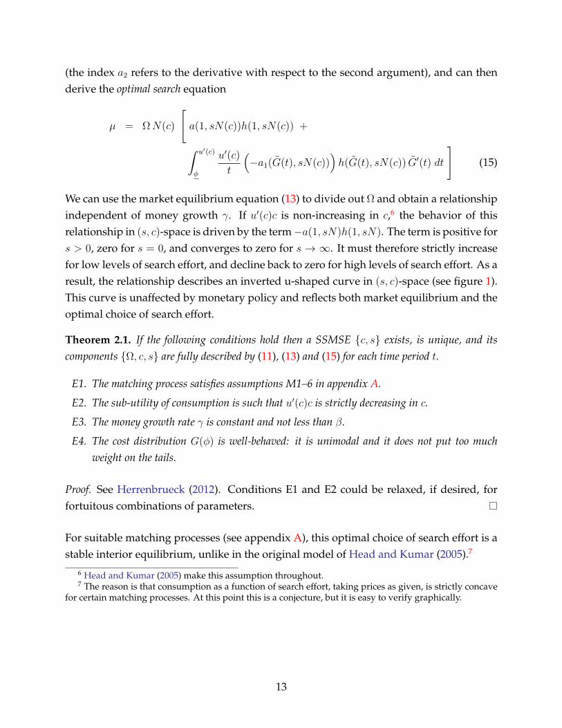
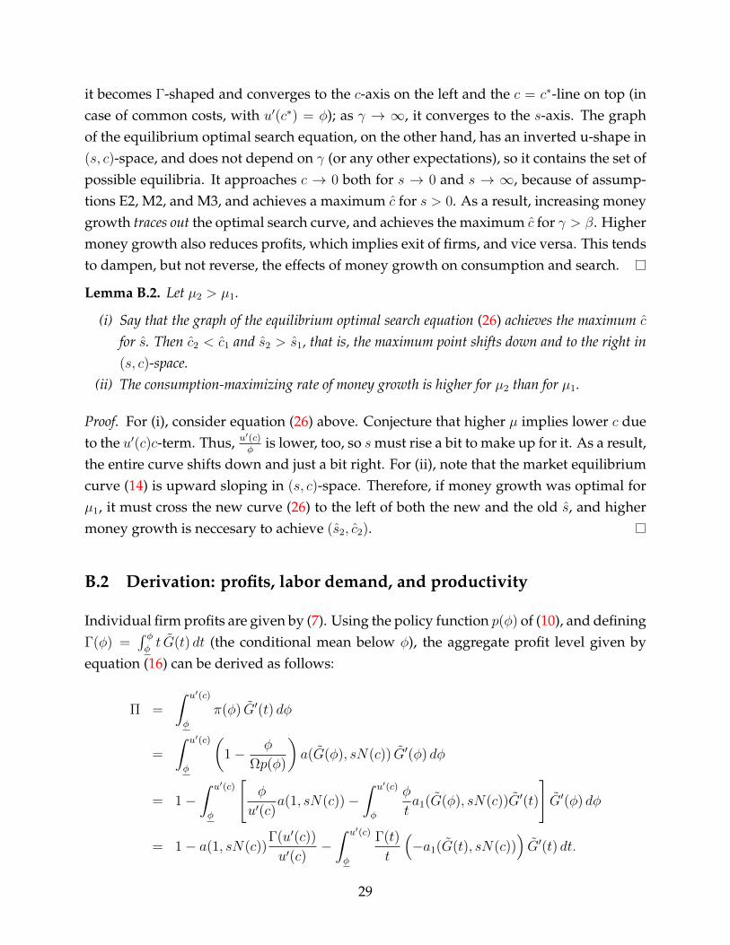
It can be shown that this curve is upward-sloping in (s, c)-space: for a given moneygrowth rate, more search effort implies more consumption. One complication arises throughthe endogenous reservation price, which implies that not all firms will be able to compete.However, this complication is not severe if the cost distribution G(φ) is well-behaved anddoes not put too much weight on the tails. Furthermore, the market equilibrium curveshifts down and right as γ increases, implying that the Friedman rule γ = β achieves themaximum level of consumption when search effort is fixed (see figure 1).5

Optimal search

The Friedman rule is still the optimal monetary policy when search effort is socially cho-sen, by maximizing u(c) − µs subject to the constraint (14). However, the result breaksdown when households privately choose their search effort. The reason is that search ef-fort accomplishes two things: it allows buyers to pick up low-price offers, and throughthat, it constrains the market power of the firms. The key is that because each householdis small, only the former effect is internalized. As a result, loose monetary policy createsprice dispersion and forces buyers to search harder. The inflation tax is Pigovian for smalllevels of inflation.

Solving the households’ problem (equation (2)), privately optimal search implies thatu′(c(s))c′(s) = µ, taking the distribution of prices F (p) as given. Details of the deriva-tion are in Herrenbrueck (2012); we need to define the auxiliary function

h(F, η) =

∫ F

0

a2(z, η)

a(z, η)dz

5 Formally, the Friedman rule is defined by a nominal interest rate of zero, which can be implementedin a variety of ways (Lagos, 2010), but which is commonly taken to be equivalent to shrinking the moneysupply at the rate of time preference.

12

(the index a2 refers to the derivative with respect to the second argument), and can thenderive the optimal search equation

µ = ΩN(c)

[a(1, sN(c))h(1, sN(c)) +

∫ u′(c)

φ

u′(c)

t

(−a1(G(t), sN(c))

)h(G(t), sN(c)) G′(t) dt

](15)

We can use the market equilibrium equation (13) to divide out Ω and obtain a relationshipindependent of money growth γ. If u′(c)c is non-increasing in c,6 the behavior of thisrelationship in (s, c)-space is driven by the term−a(1, sN)h(1, sN). The term is positive fors > 0, zero for s = 0, and converges to zero for s → ∞. It must therefore strictly increasefor low levels of search effort, and decline back to zero for high levels of search effort. As aresult, the relationship describes an inverted u-shaped curve in (s, c)-space (see figure 1).This curve is unaffected by monetary policy and reflects both market equilibrium and theoptimal choice of search effort.

Theorem 2.1. If the following conditions hold then a SSMSE c, s exists, is unique, and itscomponents Ω, c, s are fully described by (11), (13) and (15) for each time period t.

E1. The matching process satisfies assumptions M1–6 in appendix A.

E2. The sub-utility of consumption is such that u′(c)c is strictly decreasing in c.

E3. The money growth rate γ is constant and not less than β.

E4. The cost distribution G(φ) is well-behaved: it is unimodal and it does not put too muchweight on the tails.

Proof. See Herrenbrueck (2012). Conditions E1 and E2 could be relaxed, if desired, forfortuitous combinations of parameters.

For suitable matching processes (see appendix A), this optimal choice of search effort is astable interior equilibrium, unlike in the original model of Head and Kumar (2005).7

6 Head and Kumar (2005) make this assumption throughout.7 The reason is that consumption as a function of search effort, taking prices as given, is strictly concave

for certain matching processes. At this point this is a conjecture, but it is easy to verify graphically.

13

Free entry

Define the function Γ(φ) =∫ φφt G(t) dt (the conditional mean below φ). Then aggregate

profits are, in constant-money terms:

Π = 1− a(1, sN(c))Γ(u′(c))

u′(c)−∫ u′(c)

φ

Γ(t)

t

(−a1(G(t), sN(c))

)G′(t) dt (16)

Firms can enter into the market if they pay a fee fee kE < 1, assessed in constant-moneyterms8 and each period.9 Assume that this entry fee is distributed among households,i.e. added to equation (3). Firms will enter if their expected profits exceed the entry fee,and exit otherwise. Crucially, firms will only learn their cost after paying the entry fee.Therefore, the free-entry condition is:

Π = N(c)kE

= NG(u′(c))kE (17)

The SMSE is now summarized by Ω, c, s, N), which solve equations (11), (13), (15), and(17). Dividing Ω and N out of equation (15) using equations (13) and (17) yields a curve in(sN, c)-space that is unaffected by money growth. The market equilibrium equation (13)depends only on sN , not on s or N directly. The only difference is that the new optimalsearch curve is a bit flatter than previously, but it has the same shape, and the SSMSEexists and is unique under the same conditions as before, with the addition of kE < 1 toensure that some firms do enter.

Effects of inflation

In a flexible-price model like this one, money is neutral and only expectations of futuremoney growth affect the value of money, Ω, and therefore the real economy. This is eas-ily obscured when focusing on steady states alone, but worth keeping in mind for thefollowing analysis. More details and proofs are provided in Herrenbrueck (2012).

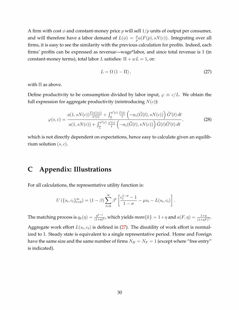
As shown in appendix B.1, there exists a consumption-maximizing rate of money growthγ > β. Consumption is increasing in γ for β < γ < γ and decreasing in γ otherwise. Searcheffort is increasing in γ throughout. With free entry, the number of firms is decreasing inγ (see figure 2).

8 The qualitative results are the same if the cost is assessed in labor terms.9 Like in Melitz (2003), this simplifies the analysis, but ignores the effect of interest rates on funding costs.

14

If we define the aggregate nominal price level by P = Mc

, we can also discuss the effectsof money growth on inflation. Clearly, in a steady state, money growth must equal in-flation. Considering a transition from one steady state into another, however, they maybe quite separate, because of the effect on consumption growth. Consider a world whereexpectations of money growth are so low that consumption would increase with highermoney growth (γ < γ). In a new steady state with lower expectations of money growth,consumption would be lower, too. By the definition of the price level P , price inflationthen falls by less than money growth, and may even rise in rare cases, between the twosteady states.

Lastly, it is worth paying attention to the interaction between the search cost µ and theoptimal rate of money growth in steady state. A higher µ shifts the optimal search curvedown in (s, c)-space, implying a lower level of consumption for a given search effort.Assume that γ was previously such that the consumption maximum was achieved. As themarket equilibrium curve slopes up for any level of γ, the new consumption maximum isto the right and below the formerly optimal market equilibrium curve. Consequently, theoptimal rate of inflation is increasing in the search cost µ; and the same thing is true forthe cost of firm entry, kE , when there is free entry of firms.

2.3 The open economy

Let there be two countries, Home and Foreign, and denote Home variables with the sub-script H and Foreign variables with the subscript F . Define the nominal exchange rateE in terms of Home currency divided by Foreign currency, and define the real exchangerate using the Home and Foreign price levels: ε = E PF

PH(in terms of Home consumption

divided by Foreign consumption). By the definition of the price level P , this implies:

ε = EMF cHMH cF

The nominal and real exchange rates are of most practical interest, but the model is mucheasier to solve in terms of the wage-based exchange rate (in terms of Home labor dividedby Foreign labor; or utility, since the disutility of labor was normalized to 1), because thisis the exchange rate relevant for firms’ competition. Define

v = EMF wFMH wH

(18)

= εcF ΩH

cH ΩF

.

15

Trade proceeds as follows. Firms can advertise prices in either country, but denominatedin local currency.10 From the point of view of the consumer, domestic and imported goodsare indistinguishable. There is also no bias on how likely a consumer is to observe adomestic or importing firm. Whenever a consumer likes the price and wants to purchasethe good, the firm produces the good and ships it to they buyer. Of course, goods cannotbe shipped costlessly. Trade costs are assessed in the familiar iceberg form: in order to sellx units of a good in a foreign market, a firm needs to ship τx units from home, with τ > 1.So while there is no bias against imported goods, domestic firms are able to charge lowerprices on average than the importing competition.

In order to simplify the analysis, I assume that the cost distribution of domestic firmsis the same in each country, and that any firm can export if is able to compete abroad.Assume that the mass of potential firms is NH at Home and NF in the Foreign country.The distribution of active firms in either country is therefore:

GH(φ) =NH

NH +NF

G(φ)

G(u′(cH))+

NF

NH +NF

G( φvτ

)

G(u′(cH)vτ

)(19)

GF (φ) =NH

NH +NF

G(φvτ

)

G(u′(cF )vτ

)+

NF

NH +NF

G(φ)

G(u′(cF ))(20)

As before, the distribution of quotes a buyer recieves depends not only on his search effort,but also on the mass of active firms:

NH(cH , v) = NH G(u′(cH)) + NF G(u′(cH)

vτ) (21)

NF (cF , v) = NH G(u′(cF )v

τ) + NF G(u′(cF )) (22)

To avoid having to track the bounds of the support of the cost distribution, I assume thatG(φ) ∈ (0, 1) for all φ > 0. Existence of an equilibrium does require that the density G′(φ)

declines to zero quickly enough as φ → 0. In practice, a log-normal distribution of costsseems to work well, and so would a log-logistic or Weibull distribution.

10 This assumption is not essential for the the results of the model, but convenient. It can be motivated byassuming that households only recognize local currency as counterfeiting-proof. Alternative motivations,such as an infinitesimal cost of conducting transactions in any foreign currency (e.g. in Geromichalos andSimonovska, 2011), would deliver the same results.

16

Balance of Payments

After trading goods, firms can visit an instantaneous, perfectly competitive foreign ex-change market in order to obtain the domestic currency valued by its workers and own-ers. In steady state (or without capital markets), currency flows must exactly offset eachother. The value of Foreign currency revenue gained by Home exports must equal thevalue of Home currency revenue paid for Home imports. After substituting equation (18)for the nominal exchange rate, we obtain the balance of payments relationship:

v =ΩH

ΩF

∫ u′(cH )

vτ

0a(GH(vτt), sHNH(cH , v))G′(t) dt∫ v

τu′(cF )

0a(GF ( τ

vt), sFNF (cF , v))G′(t) dt

NF G( vτu′(cF ))

NH G(u′(cH)vτ

)(23)

Equilibrium, solving for equilibrium, and comparative statics

Definition 2. An open-economy steady-state equilibrium consists of the seven endoge-nous sequences ΩHt,ΩFt, cHt, cFt, sHt, sFt, vt∞t=0 which solve the following equations:

I. Equation (11) for Home. It links ΩH and cH .II. Equation (11) for Foreign. It links ΩF and cF .

III. Equation (13) for Home, replacing G( · ) by (19) and N(c) by (21). It links ΩH , cH , sH ,and v.

IV. Equation (13) for Foreign, replacing G( · ) by (20) and N(c) by (22). It links ΩF , cF ,sF , and v.

V. Equation (15) for Home, replacing G( · ) and N(c) as for (III.). It links ΩH , cH , sH , andv.

VI. Equation (15) for Foreign, replacing G( · ) and N(c) as for (IV.). It links ΩF , cF , sF ,and v.

VII. Equation (23), which links all seven endogenous variables.

A numerical solution to this system involves six numerical integrals, which may have toevaluated many times as a solution is approached. This procedure can be sped up dramat-ically by evaluating each integral on a grid of endogenous variables and interpolating theequation on this grid. Because of the curse of dimensionality, the number of endogenousvariables involved in each equation should be as small as possible.

For example, steady state solutions can be found as follows. Firstly, replace all instancesof ΩH and ΩF using equations (I.) and (II.). Secondly, while equation (VII.) still involves

17

five endogenous variables, it can be split into two parts, the first involving the home en-dogenous variables plus v, the second one involving the foreign endogenous variablesplus v. There are six integrals left, each needing to be evaluated on a three-dimensionalgrid. If the grid contains p points in one dimension, 6 × p3 integrals have to be evaluatedin order to create a manageable system of five interpolated equations in five variables.After this prodedure, solutions can be found easily. The productivity parameters have tobe hard-coded into the interpolation, but the money growth and search cost parameterscan be introduced into the last stage, which makes their comparative statics very easy toexamine.

Unfortunately, free entry would require two additional integrals (for profits), and the di-mension of each integral would go up to five when NH and NF are made endogenous. Soa grid that contains p points in each dimension would require 8× p5 integral evaluations.For this reason, free entry would complicate the computation considerably.

Turning to the effects of money growth: An increase in the Home money growth rate γHincreases both Home and Foreign search effort (although naturally, Home search effortresponds more strongly if τ > 1). It increases Home consumption when γH is low anddecreases it when γH is high, just as in autarky. It increases the real exchange rate (aHome depreciation), because it increases Home search effort which reduces the marketpower of Foreign firms selling at Home, reducing their revenue, and balance of paymentsthen forces a depreciation (see figure 3).

As the increase in Home money growth always increases Home search effort, it shifts pro-duction to the more efficient firms. As a result, higher Home money growth reduces Homelabor demand and increases Home productivity (defined as production divided by laborinput; see appendix B.2) throughout. The effect on Foreign productivity is ambiguous andsmall.

Unlike in the closed economy, higher Home money growth only has a small, but stillnegative, effect on Home profits. It has a much larger negative effect on Foreign profits,however. (With free entry, “profits” could be substituted by “the number of firms”, andthe rest of the results would not change qualitatively.)

When search effort is fixed, which is probably the correct model in the short run, theeffects are very different. Higher Home money growth γH decreases Home consumptionthroughout, barely affects Foreign consumption, and decreases both the constant-moneynominal and real exchange rates (Home imports fall, but their value relative to Homeexports has to be constant to maintain balance of payments). Because they rely on the

18

strong assumption of balance of payments, these short-run exchange-rate effects probablywould not survive the introduction of capital markets into the model.

With the effect of Home money growth on home consumption as described, consumptionis maximized with a money growth rate above the Friedman rule. This consumption-maximizing Home money growth rate increases in µH (as was the case in autarky), isbarely affected by µF , and decreases in Foreign money growth γF . Consequently, whencountries play a non-cooperative game, each choosing the money growth rate with thegoal of maximizing domestic consumption, the game has an interior Nash equilibrium.

3 Welfare implications

In this section, I analyze the steady-state effects of constant money growth on the house-hold utility function (1). Steady state implies that we can focus on a single representativeperiod.

3.1 Costs and benefits of money growth

Higher steady-state money growth has the following effects in the closed economy:

• The inflation tax increases market power, which implies lower consumption and/ormore search.

• The inflation tax increases the real wage, because payment compensates workers forthe fixed disutility of production, and payment loses value. This higher real wageimplies lower production.

• When households choose their search effort, they only consider the internal effectof better offers, but not the external effect of lower market power. They will tendto search too little. Through stimulating search effort, money growth increases con-sumption.

• Higher search effort directly decreases utility (“shoe-leather cost”).

• Higher search effort shifts matches to the more efficient firms, which implies higherconsumption and/or lower labor effort.

Two second-order effects need to be mentioned, too:

19

• With heterogeneous firms, higher consumption lowers the reservation wage, whichallows fewer firms to compete and reduces matching. This will tend to dampen theeffects of money growth on consumption.

• With free entry, lower search effort implies more profits and induces entry, and viceversa. This will tend to dampen the effects of money growth on consumption andsearch effort.

In conclusion, very low money growth implies very low consumption and therefore verylow utility. Moderate money growth yields a maximum of consumption, and even highermoney growth reduces consumption again. As money growth increases search effortthroughout, the resulting increase in “shoe-leather costs” suggests that the optimal rateof optimal money growth is below the level that maximizes consumption. On the otherhand, when firms are heterogeneous, higher money growth increases productivity andreduces the amount of labor required in production, which suggests that the optimal rateof money growth is above the level that maximizes consumption. Which effect dominatescan only be decided numerically and empirically.

In the open economy, the following effects of an increase in the Home money growth rateneed to be considered additionally:

• Higher Home search effort reduces the market power of Foreign exporters, and doesnot affect Home exports abroad. The result is an improvement in the terms of trade.

• Higher real wages at Home exploit market power abroad.

Both effects increase Home consumption and reduce Foreign consumption. As a result,the optimal money growth rate in the open economy will be higher that in the closedeconomy, but at the expense of trading partners (see figure 4).11

3.2 Coordination

As discussed among the comparative statics of the international economy, the consumption-maximizing Home money growth rate is decreasing in the Foreign money growth rate.One can verify numerically that this also holds for the welfare-maximizing Home moneygrowth rate, although only globally. This implies that the joint welfare function obtainedby adding both countries’ welfare functions is generally submodular in (γH , γF ), and

11 In the words of Corsetti (2006), inflation is a beggar-thy-neighbor policy.

20

while it may have multiple Nash equilibria in principle, they must lie close together andmay be indistinguishable in practice.

Higher Home money growth unambiguously decreases Foreign consumption, increasesForeign search effort, and increases Foreign labor use. The outcome is unambiguouslynegative for the Foreign country. The Home welfare function is smooth, at least in theneighborhood of any equilibrium, if the functions u(c), G(φ), and a(z, s) are smooth.Therefore, the Home country would increase joint welfare by reducing money growth alittle bit from any Nash equilibrium level. At very low levels of home money growth, how-ever, Home welfare rises faster than Foreign welfare falls with a small increase in Homemoney growth. Consequently, there exists at least one combination of money growth ratesthat maximizes joint welfare, and at least one country must set money growth below thelevel that would, given the other country’s money growth rate, maximize national wel-fare.

Clearly, monetary coordination is then the best outcome for the two countries, and thedifference may be significant. As an example, consider the parameters G ∼ logN(1, 1

6),

τ = 1.3, σ = 2, β = 0.98, µH = µF = 0.008. The unique Nash equilibrium is γH = γF = 1.1

(nominal interest rates of 12%), while the joint optimum is γH = γF = 1.04 (nominalinterest rates of 6%, half as high).

3.3 Currency union

Consider another example, with two countries that are of equal size and alike in everyway, except that µH > µF .12 Then any Nash equilibrium and any joint optimum mustsatisfy γH > γF . With the same parameters as above, except that µH = 0.016 is twice ashigh as µF = 0.008, the optimal money growth rates are as follows:

• Nash equilibrium: γH = 1.16, γF = 1.05.

• Joint optimum: γH = 1.12, γF = 1.02.

• Symmetric joint optimum: γH = γF = 1.05.

A currency union is defined by the criterion γH = γF .13 The numerical example abovedemonstrates why a currency union can be disadvantageous in the wrong circumstances.

12 While µ is the disutility of search, it has similar static effects as the cost of firm entry kE . As the two-country model is harder to solve with free entry, I understand µ as standing in for kE , too, in this exercise.

13 The exact conversion rate E is immaterial, as in the long run, households holds the relative amount ofcurrency that will achieve balance of payments. Certainly, the transition path may matter for welfare, butthe present paper is concerned with steady states only.

21

At the joint symmetric optimum, the welfare difference between home and foreign is anorder of magnitude larger than in the joint optimum (see figure 4). The joint welfare loss issmall, but the foreign country gains from the currency union and the home country loses,even when joint welfare is the criterion used to determine the money growth rate.

If we believe that search effort does not respond quickly, because consumers need to keeplearning the price distribution and firms need to keep learning the sales function (whichdepends on search effort), the transition dynamics into currency union become interesting.With the given parameters, consider a move by the Home country from γH = 1.12 toγH = 1.05, while the Foreign country moves from γF = 1.02 to γF = 1.05. As long assearch effort remains fixed, Home consumption rises by a dramatic 7 or 8%, while Foreignconsumption declines very slightly (probably too slightly to be distinguished from noise).

As soon as search effort adjusts, however, Foreign search effort rises slightly while Homesearch effort collapses by more than two thirds. As a result, Foreign consumption in-creases by 2 or 3%, while Home consumption falls by 8 or 9%, below the initial level. Inaddition, Foreign productivity increases and Home productivity falls. Together, these ef-fects imply the result discussed above: Foreign wins, Home loses, even when joint welfareis used to determine the monetary growth rate in the currency union (see figures 3 and 4).

To make matters worse, the outcome is easily mis-diagnosed as due to different rates ofproductivity growth at home and abroad. What really happens is that the decline in Homesearch effort leads to less efficient matches, causing measured Home productivity to fall,while the increase in Foreign search effort causes Foreign productivity to rise.

4 Conclusion and discussion

In this paper, I use the monetary search model of Herrenbrueck (2012) to study monetarypolicy in an international setting. The optimal steady-state money growth rate depends onthe fundamendals of the economy, and it can be calculated numerically. Higher inflationnecessarily has adverse effects on trading partners (a “beggar-thy-neighbor” policy), soinflation will be lower and welfare will be higher when policy is coordinated.

However, when countries with different fundamentals join a currency union which choosesits inflation rate to maximize joint welfare, at least one country must raise its inflation raterelative to the coordination outcome, and at least one country must lower it. A countrythat raises its inflation rate gains twice: first, a higher inflation rate relative to optimal coor-dination must raise its domestic welfare, while second, lower inflation in its trading part-

22

ner countries improves its terms of trade. On the other hand, by the same mechanisms,a country that lowers its inflation rate to join a currency union loses twice. Certainly, acurrency union may or may not improve welfare compared with a non-cooperative Nashequilibrium, or when all members reduce their inflation rates, so it may still be a goodidea when coordination is not feasible for some reason.

In future work, I plan to calibrate the model to the Eurozone economy of the 1990s and2000s and compute the welfare outcomes precisely. Preliminary evidence presented inFigure 5 suggests that the model can contribute to explaining the see-saw macroeconomicdivergence of two parts of the Eurozone since the early 1990s (here named North andSouth, defined next to the graph), when plans to form a currency union congealed intofact. Panel (a) shows that until 1994, the economies of the North and the South movedtogether compared to a rest-of-the-developed-world aggregate, but that after 1995 (whenthe Euro was formally announced), South first catches up to North but then falls far be-hind. This is exactly consistent with my model; if search effort and the number of firmstake a few years to adjust to the new steady state, a reduction in inflation in the Southrelative to the North will initially result in relative growth in the South as the inflation taxis reduced, but will ultimately result in relative decline in the South as search effort falls.

Panel (b) shows that indeed, monetary policy tightened in the South relative to the Northfrom the early 1990s until convergence was achieved in 1998. Furthermore, the financialcrisis of 2008-09 or the worries about a potential sovereign debt crisis, which began in 2009and accelerated in 2010, appear to be consequences rather than causes of the macroeco-nomic imbalances. Relative GDP of the South peaked in 2002, and relative consumption(not graphed) peaked in 2006. Instead, I propose that the turnaround of relative outputmay be a late consequence of the relative monetary tightening in the 1990s.14 Currently,however, I have no microeconomic evidence that search effort was the channel of this see-saw divergence. In future work, I plan to study data on price dispersion, sales dispersion,and firm entry, which together should provide a clearer picture of search effort and firmentry in the crucial period of the 2000s.

Whereas the disutility of search effort seems hard to reliably compare accross countries,data on the cost of firm entry and operation is readily available. According to the Ease ofDoing Business Index (World Bank, 2011), the countries making up the North as defined inFigure 5 average a worldwide rank of 24.5, and the countries of the South average a rank of63.6 (weighted by 2008 nominal GDP). The conclusions of the model are clear: the optimal

14 The German welfare reforms of 2002 are also an unlikely cause of the turnaround; the graphs looksubstantially the same with Germany excluded.

23

inflation rate is higher in the South than in the North, and while the overall downwardtrend of nominal interest rates in the 1990s may have been good for both regions, theconvergence of interest rates was likely harmful for the South.

References

Sascha Becker and Dieter Nautz. Inflation, price dispersion and market integrationthrough the lens of a monetary search model. Discussion Papers 2010/2, Free Uni-versity Berlin, School of Business & Economics, 2010. URL http://ideas.repec.org/p/zbw/fubsbe/20102.html.

Sascha S. Becker. What drives the relationship between inflation and price dispersion?market power vs. price rigidity. SFB 649 Discussion Papers SFB649DP2011-019, Son-derforschungsbereich 649, Humboldt University, Berlin, Germany, March 2011. URLhttp://ideas.repec.org/p/hum/wpaper/sfb649dp2011-019.html.

Aleksander Berentsen, Guillaume Rocheteau, and Shouyong Shi. Friedman meets hosios:Efficiency in search models of money. Economic Journal, 117(516):174–195, 01 2007. URLhttp://ideas.repec.org/a/ecj/econjl/v117y2007i516p174-195.html.

Kenneth Burdett and Kenneth L Judd. Equilibrium price dispersion. Economet-rica, 51(4):955–69, July 1983. URL http://ideas.repec.org/a/ecm/emetrp/v51y1983i4p955-69.html.

Kenneth Burdett and Dale T Mortensen. Wage differentials, employer size, and un-employment. International Economic Review, 39(2):257–73, May 1998. URL http://ideas.repec.org/a/ier/iecrev/v39y1998i2p257-73.html.

Mustafa Caglayan, Alpay Filiztekin, and Michael T. Rauh. Inflation, price dispersion,and market structure. European Economic Review, 52(7):1187–1208, October 2008. URLhttp://ideas.repec.org/a/eee/eecrev/v52y2008i7p1187-1208.html.

Giancarlo Corsetti. Openness and the case for flexible exchange rates. Research in Eco-nomics, 60(1):1–21, March 2006. URL http://ideas.repec.org/a/eee/reecon/v60y2006i1p1-21.html.

Giancarlo Corsetti and Paolo Pesenti. The simple geometry of transmission and stabiliza-tion in closed and open economies. In NBER International Seminar on Macroeconomics2007, NBER Chapters, pages 65–116. National Bureau of Economic Research, Inc, Win-ter 2009. URL http://ideas.repec.org/h/nbr/nberch/3000.html.

Ben Craig and Guillaume Rocheteau. Inflation and welfare: A search approach. Journal ofMoney, Credit and Banking, 40(1):89–119, 02 2008. URL http://ideas.repec.org/a/mcb/jmoncb/v40y2008i1p89-119.html.

24

Michael B. Devereux and Shouyong Shi. Vehicle currency. Globalization and MonetaryPolicy Institute Working Paper 10, Federal Reserve Bank of Dallas, 2008. URL http://ideas.repec.org/p/fip/feddgw/10.html.

Athanasios Geromichalos and Ina Simonovska. Asset liquidity and international portfo-lio choice. NBER Working Papers 17331, National Bureau of Economic Research, Inc,August 2011. URL http://ideas.repec.org/p/nbr/nberwo/17331.html.

Allen Head and Alok Kumar. Price dispersion, inflation, and welfare. InternationalEconomic Review, 46(2):533–572, 05 2005. URL http://ideas.repec.org/a/ier/iecrev/v46y2005i2p533-572.html.

Allen Head and Beverly Lapham. Search, market power, and inflation dynamics. 2006Meeting Papers 559, Society for Economic Dynamics, December 2006. URL http://ideas.repec.org/p/red/sed006/559.html.

Lucas M. Herrenbrueck. A general equilibrium open-economy model with money, en-dogenous search, and heterogeneous firms. Working paper, University of California,Davis, 2012.

Ricardo Lagos. Some results on the optimality and implementation of the friedman rule inthe search theory of money. Journal of Economic Theory, 145(4):1508–1524, July 2010. URLhttp://ideas.repec.org/a/eee/jetheo/v145y2010i4p1508-1524.html.

Victor E Li. The optimal taxation of fiat money in search equilibrium. International Eco-nomic Review, 36(4):927–42, November 1995. URL http://ideas.repec.org/a/ier/iecrev/v36y1995i4p927-42.html.

Andre Meier. Still minding the gap - inflation dynamics during episodes of persistentlarge output gaps. Working Paper WP/10/189, IMF, August 2010. URL http://www.imf.org/external/pubs/ft/wp/2010/wp10189.pdf.

Marc J. Melitz. The impact of trade on intra-industry reallocations and aggregate industryproductivity. Econometrica, 71(6):1695–1725, November 2003. URL http://ideas.repec.org/a/ecm/emetrp/v71y2003i6p1695-1725.html.

Dale T. Mortensen. A comment on ”price dispersion, inflation, and welfare” by a. headand a. kumar. International Economic Review, 46(2):573–578, 05 2005. URL http://ideas.repec.org/a/ier/iecrev/v46y2005i2p573-578.html.

Robert A. Mundell. A theory of optimum currency areas. The American Economic Review,51(4):657–665, September 1961. URL http://www.jstor.org/stable/1812792.

Robert A. Mundell. Uncommon arguments for common currencies. In H.G. Johnson andA.K. Swoboda, editors, The Economics of Common Currencies, pages 114–132. Allen andUnwin, 1973.

Shouyong Shi. A divisible search model of fiat money. Econometrica, 65(1):75–102, January1997. URL http://ideas.repec.org/a/ecm/emetrp/v65y1997i1p75-102.html.

25

Shouyong Shi. A microfoundation of monetary economics. Working Papers tecipa-211,University of Toronto, Department of Economics, March 2006. URL http://ideas.repec.org/p/tor/tecipa/tecipa-211.html.

Liang Wang. Inflation and welfare with search and price dispersion. Working Papers201113, University of Hawaii at Manoa, Department of Economics, July 2011. URLhttp://ideas.repec.org/p/hai/wpaper/201113.html.

World Bank. Ease of doing business index, 2011. URL http://www.doingbusiness.org/rankings.

Randall D. Wright, Lucy Qian Liu, and Liang Wang. On the ’hot potato effect’ of inflation:Intensive versus extensive margins. Working Paper 09-040, PIER, November 2009. URLhttp://ssrn.com/abstract=1501132.

Cathy Zhang. Information costs and international currencies. Working paper, Uni-versity of California, Irvine, March 2012. URL http://laef.ucsb.edu/pages/conferences/sam12/papers/zhang.pdf.

26

A Appendix: Matching

The assumptions on the matching process sufficient for the results in this paper are:

M1. Q(k|η) is a cumulative distribution function with support 1 . . . K, where K ∈2 . . .∞. qk(η) is used to denote the probability mass function.

M2. q1(η) ∈ (0, 1) for all η > 0, and q1(0) = 1.M3. When η′ > η, Q(k|η′) < Q(k|η): the distribution of quotes with higher search effort

strictly first order stochastically dominates the one with lower search effort.M4. Q(k|η) is differentiable in η.M5. q′1(η) is bounded as s→ 0.M6. There exists an ε > 0 such that the series

∑Kk=1 k

2+ε (q′k(η))2 converges for any η > 0,and that the series limit approaches 0 as η →∞.

For quantitative results, I use the geometric matching process qk(η) = ηk−1

(1+η)k, which sat-

isfies assumptions M1–6.15 Intuitively, it can be characterized by the buyer flipping a(loaded) coin until it comes up tails, and then getting one quote for each flip. But all of thefollowing matching processes give quantitatively similar results:

Binary: q1 = 1 − s, q2 = s, K = 2, used by Head and Kumar (2005). Advantage: ifbuyers could choose each qk separately, they would choose to mix between q1 and q2

only. Disadvantage: consumption is a convex function of search effort, requiring amixed strategy equilibrium for the choice of search effort. Furthermore, equilibriumis degenerate if µ is too small or too large.

Poisson: qk = e−ηηk−1

(k−1)!, K = ∞, suggested by Mortensen (2005) and used by Head and

Lapham (2006). Very similar to the geometric, perhaps a bit less intuitive.

Log-series: qk = 1log(1+η)

( η1+η )

k

k, K = ∞, used in earlier versions of the present paper.

Slightly simpler math than the geometric, but less intuitive.

B Appendix: Proofs

Proof of lemma 2.1: (Based on equation (34) in Burdett and Mortensen (1998).) We can rank

π(p1;φ1) ≥ π(p2;φ1) > π(p2;φ2) ≥ π(p1;φ2) (24)15 M1–M5 are easy to see. For ε = 0.5, the series limit in M6 has a closed-form solution, and it does

converge to 0 as s→∞.

27

The first and last inequality follow from profit maximization. The middle inequality fol-lows from φ1 < φ2. Subtracting the fourth term from the first, and the third term from thesecond, and rearranging, we get

p2

a(p2)≥ p1

a(p1)(25)

As F (p) is a continous c.d.f. with connected support, it is strictly increasing on its sup-port. From its definition, it is easy to see that a(F ) is a strictly decreasing function of F .Therefore, a(F (p)) is a strictly decreasing function of p on the support of F .

Proof of lemma 2.2: p(φ) solves the FOC. Regarding the boundary condition: either p isbinding for some sellers, in which case the marginal seller will charge p and make zeroprofits. Or the least efficient seller is still able to compete, but must charge the highestprice by the ranking condition; then, however, no buyer with another choice will buyfrom this seller. Therefore, a buyer who is willing to buy from this seller will accept anyprice up to p, and the least efficient seller will charge p.

B.1 Effects of inflation

Lemma B.1. In a steady state of a SSMSE, the Friedman rule γ = β implies c = 0, γ > β impliesc > 0 and γ → ∞ implies c → 0. Therefore, the consumption-maximizing rate of money growthsatisfies γ > β.

Proof. For simplicity, keep the number of firms fixed. But the lemma also holds with freeentry.

Divide optimal search equation (15) by the market equilibrium equation (13) to obtain(writing N instead of N(c) for simplicity):

µ = Nu′(c)ca(1, sN)h(1, sN) +

∫ u′(c)φ

u′(c)t

(−a1(G(t), sN)

)h(G(t), sN) G′(t) dt

a(1, sN) +∫ u′(c)φ

u′(c)t

(−a1(G(t), sN)

)G(t)G′(t) dt

(26)

Consider this “equilibrium optimal search equation” together with the market equilib-rium equation (14) in (c, s)-space. The market equilibrium curve slopes upwards, crossesthe equilibrium optimal search curve exactly once, and shifts right as money growth γ

increases: faster money growth reduces the value of money, which creates market power.Constant consumption would therefore require ever-increasing search effort. As γ → β,

28

it becomes Γ-shaped and converges to the c-axis on the left and the c = c∗-line on top (incase of common costs, with u′(c∗) = φ); as γ → ∞, it converges to the s-axis. The graphof the equilibrium optimal search equation, on the other hand, has an inverted u-shape in(s, c)-space, and does not depend on γ (or any other expectations), so it contains the set ofpossible equilibria. It approaches c → 0 both for s → 0 and s → ∞, because of assump-tions E2, M2, and M3, and achieves a maximum c for s > 0. As a result, increasing moneygrowth traces out the optimal search curve, and achieves the maximum c for γ > β. Highermoney growth also reduces profits, which implies exit of firms, and vice versa. This tendsto dampen, but not reverse, the effects of money growth on consumption and search.

Lemma B.2. Let µ2 > µ1.

(i) Say that the graph of the equilibrium optimal search equation (26) achieves the maximum c

for s. Then c2 < c1 and s2 > s1, that is, the maximum point shifts down and to the right in(s, c)-space.

(ii) The consumption-maximizing rate of money growth is higher for µ2 than for µ1.

Proof. For (i), consider equation (26) above. Conjecture that higher µ implies lower c dueto the u′(c)c-term. Thus, u

′(c)φ

is lower, too, so smust rise a bit to make up for it. As a result,the entire curve shifts down and just a bit right. For (ii), note that the market equilibriumcurve (14) is upward sloping in (s, c)-space. Therefore, if money growth was optimal forµ1, it must cross the new curve (26) to the left of both the new and the old s, and highermoney growth is neccesary to achieve (s2, c2).

B.2 Derivation: profits, labor demand, and productivity

Individual firm profits are given by (7). Using the policy function p(φ) of (10), and definingΓ(φ) =

∫ φφt G(t) dt (the conditional mean below φ), the aggregate profit level given by

equation (16) can be derived as follows:

Π =

∫ u′(c)

φ

π(φ) G′(t) dφ

=

∫ u′(c)

φ

(1− φ

Ωp(φ)

)a(G(φ), sN(c)) G′(φ) dφ

= 1−∫ u′(c)

φ

[φ

u′(c)a(1, sN(c))−

∫ u′(c)

φ

φ

ta1(G(φ), sN(c))G′(t)

]G′(φ) dφ

= 1− a(1, sN(c))Γ(u′(c))

u′(c)−∫ u′(c)

φ

Γ(t)

t

(−a1(G(t), sN(c))

)G′(t) dt.

29

A firm with cost φ and constant-money price p will sell 1/p units of output per consumer,and will therefore have a labor demand of L(φ) = φ

pa(F (p), sN(c)). Integrating over all

firms, it is easy to see the similarity with the previous calculation for profits. Indeed, eachfirms’ profits can be expressed as revenue—wage*labor, and since total revenue is 1 (inconstant-money terms), total labor L satisfies: Π + wL = 1, or:

L = Ω (1− Π) , (27)

with Π as above.

Define productivity to be consumption divided by labor input, ϕ ≡ c/L. We obtain thefull expression for aggregate productivity (reintroducing N(c)):

ϕ(s, c) =a(1, sN(c))Γ(u′(c))

u′(c)+∫ u′(c)φ

Γ(t)t

(−a1(G(t), sN(c))

)G′(t) dt

a(1, sN(c)) +∫ u′(c)φ

u′(c)t

(−a1(G(t), sN(c))

)G(t)G′(t) dt

, (28)

which is not directly dependent on expectations, hence easy to calculate given an equilib-rium solution (s, c).

C Appendix: Illustrations

For all calculations, the representative utility function is:

U (st, ct∞t=0) = (1− β)∞∑t=0

βt[c1−σt − 1

1− σ− µst − L(st, ct)

].

The matching process is qk(η) = ηk−1

(1+η)k, which yields meank = 1+η and a(F, η) = 1+η

(1+ηF )2.

Aggregate work effort L(st, ct) is defined in (27). The disutility of work effort is normal-ized to 1. Steady state is equivalent to a single representative period. Home and Foreignhave the same size and the same number of firmsNH = NF = 1 (except where “free entry”is indicated).

30

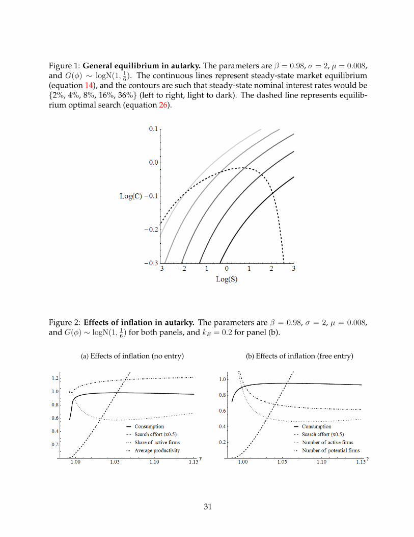
Figure 1: General equilibrium in autarky. The parameters are β = 0.98, σ = 2, µ = 0.008,and G(φ) ∼ logN(1, 1

6). The continuous lines represent steady-state market equilibrium

(equation 14), and the contours are such that steady-state nominal interest rates would be2%, 4%, 8%, 16%, 36% (left to right, light to dark). The dashed line represents equilib-rium optimal search (equation 26).

Figure 2: Effects of inflation in autarky. The parameters are β = 0.98, σ = 2, µ = 0.008,and G(φ) ∼ logN(1, 1

6) for both panels, and kE = 0.2 for panel (b).

(a) Effects of inflation (no entry) (b) Effects of inflation (free entry)

31

Figure 3: Effects of inflation in the open economy, without free entry. The parameters are β = 0.98, σ = 2, µF

= 0.008,and G(φ) ∼ logN(1, 1

6) for all panels; µ

H= 0.008 for panels (a) and (b); µ

H= 0.016 for panels (c) and (d). The vertical line

represents Foreign money growth γF

.

(a) Endogenous search effort (“long run”) (b) Fixed search effort (“short run”)

(c) Endogenous search effort (“long run”), µH µF (d) Fixed search effort (“short run”), µH µF

32

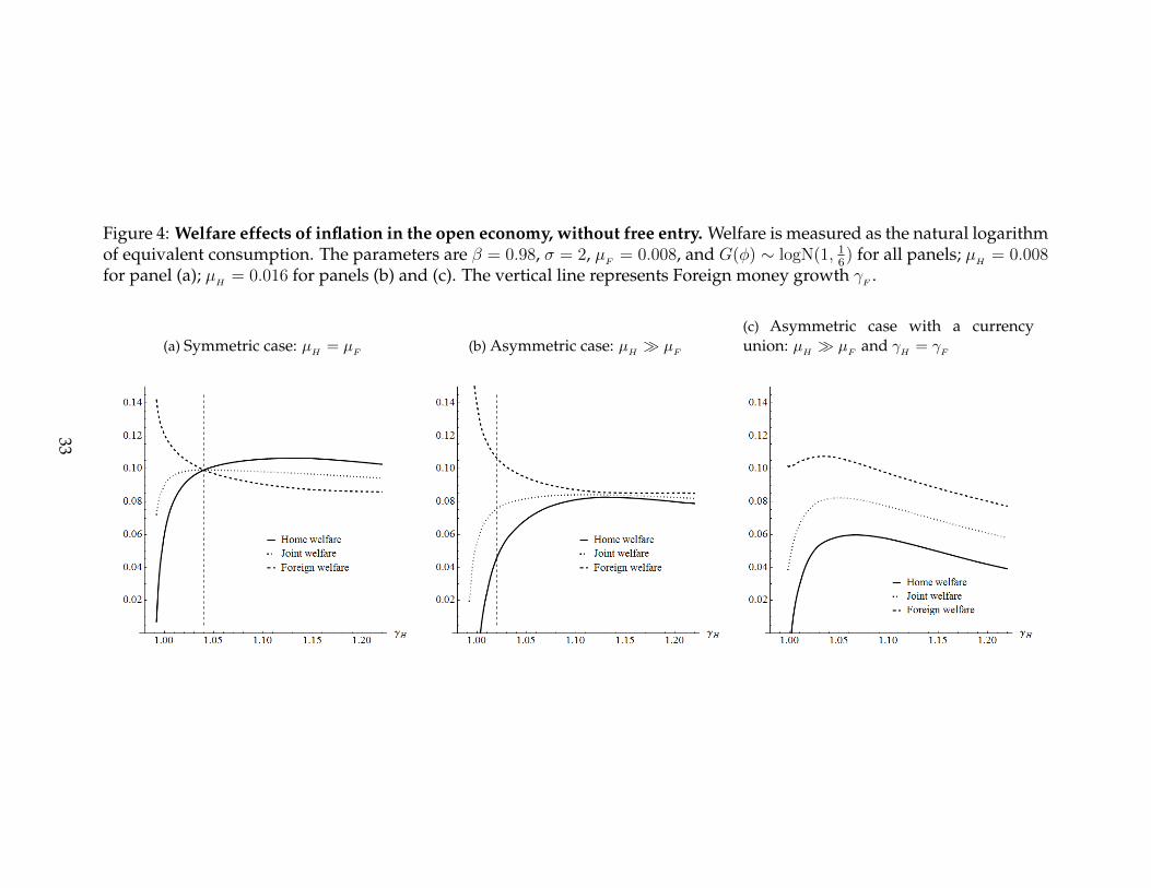
Figure 4: Welfare effects of inflation in the open economy, without free entry. Welfare is measured as the natural logarithmof equivalent consumption. The parameters are β = 0.98, σ = 2, µ

F= 0.008, and G(φ) ∼ logN(1, 1

6) for all panels; µ

H= 0.008

for panel (a); µH

= 0.016 for panels (b) and (c). The vertical line represents Foreign money growth γF

.

(a) Symmetric case: µH = µF (b) Asymmetric case: µH µF

(c) Asymmetric case with a currencyunion: µH µF and γH = γF

33

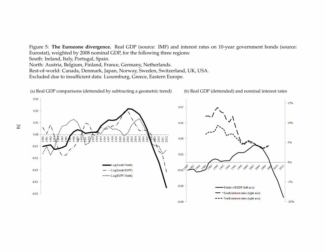
Figure 5: The Eurozone divergence. Real GDP (source: IMF) and interest rates on 10-year government bonds (source:Eurostat), weighted by 2008 nominal GDP, for the following three regions:South: Ireland, Italy, Portugal, Spain.North: Austria, Belgium, Finland, France, Germany, Netherlands.Rest-of-world: Canada, Denmark, Japan, Norway, Sweden, Switzerland, UK, USA.Excluded due to insufficient data: Luxemburg, Greece, Eastern Europe.

(a) Real GDP comparisons (detrended by subtracting a geometric trend) (b) Real GDP (detrended) and nominal interest rates

34