Embed Size (px)
Citation preview

February, 1969 RE M.I.T. DSR Project 76265 NASA Grant NGL-22-009-124
A
OPTIMAL OUTPUT-FEEDBACK CONTROLLERS FOR LINEAR SYSTEMS
William S. Levine
Electronic Systems Laboratory
MASSACHUSETTS INSTITUTE OF TECHNOLOGY, CAMBRIDGE, MASSACHUSETTS 02l39
Department of Electrical Engineering
https://ntrs.nasa.gov/search.jsp?R=19690011727 2020-03-12T10:44:01+00:00Z

February, 1969 Report ESL-R-374 Copy No.
OPTIMAL OUTPUT -FEEDBACK CONTROLLERS FOR LINEAR SYSTEMS
by
William S. Levine
This report consists of the unaltered thesis of William S. Levine, submitted in partial fulfillment of the requirements for the degree of Doctor of Philosophy a t the Massachusetts Institute of Technology in January, 1969. This research was car r ied out a t the M.1, T. Electronic Systems Laboratory with support extended by the National Aeronautic and Space Administration under Research Grant No. NGL-22-009( 124), M. I. T. DSR Project No. 76265.
Electronic Sys tern s Lab0 rat0 r y Department of Electric a1 Engineering Massachusetts Institute of Technology
C amb ridg e , Mas s ac hus e tts 02 1 3 9

OPTIMAL OUTPUT-FEEDBACK CONTROLLERS FOR LINEAR SYSTEMS
WILLIAM SILVER LEVINE
Submitted to the Department of Electrical Engineering on January 22, 1969 in partial fulfillment of the requirements for the Degree of Doctor of Philosophy.
ABSTRACT
This research is concerned with the optimal control of linear systems with respect to a quadratic performance criterion. problem is formulated with the additional constraint that the control vector u(t) is a linear function of the output vector y( t ) (u(t) = -F(t)y(t)) - ra ther &an of the state vector x(t). - F"'(t) is then chosen to minimize an "averaged" quadratic performance criterion.
The optimization
The optimal fegdbacx mat&
The necessary conditions provided by the matr ix minimum- principle aqe used to determine. the optimal feedback gain matr ix F'"(t). This - F:''(t) is then shown to satisfy the Hamilton-Jacobi equa t sn thereby demonstrating that it is a t least locally optimal. tence of an optimal feedback gain matrix is proven.
A computer algorithm is developed to facilitate the calculation of F'"(t) for practical problems. the solution of several examples.
In addition, the exis-
This algorithm is programmed and used Tn
Finally, a time-invariant version of the above prphlem is formulated and solved. Again an algorithm for computing F' (in this case, a constant matrix) is suggested. In addition, several examples a r e solved.
Thesis Supervisor : Michael Athans Title : Associate Professor of Electrical Engineering
.. -11-

ACKNOWLEDGMENT
It is a great pleasure to be able to thank Prof. Michael Athans for his many contributions to the author's education. His encouragement and enthusiasm, his technical insight and suggestions have played a funda- mental role in my graduate training. He has been an "optimal" thesis advisor.
It is also a pleasure to thank Professors Roger Brockett and Leonard A. Could for their many constructive cri t icisms and comments while serving as readers for this thesis. the technical contents and improved the exposition of this research.
Their suggestions have enriched
Many of the author's colleagues have also contributed to these results. In particular, Prof. J. C. W i l l e m s , Prof. A. H. Levis, Dr. D. L. Kleinman, T. Fortmann, S. G. Greenberg and J. H. Davis deserve special mention.
My wife Shirley has made essential, although entirely non-technical, contributions to this research.
I would also like to thank Carol Hewson of the ESL Publications Staff for her rapid and accurate typing of the final report and Arthur Giordani of the ESL Drafting Department for his help with the figures.
This research was car r ied out at the M. I. T. Electronic Systems Lab- oratory with support provided in par t by the NASA Electronic Research Center under Grant NGL-22-009( 124), and in par t by the U. S. Depart- ment of Transportation under Contract C-85-65.

CHAPTER I
CHAPTER I1
2. 1
2.2
2. 3
2 .4
2. 5
CHAPTER I11
3 . 1
3. 2
3.3
CHAPTER IV
4. 1
4.2
4.3
4.4
4. 5
CHAPTER V
APPENDIX A
APPENDIX B
REFERENCES
CONTENTS
INTRODUCTION page 1
THEORETICAL RESULTS - OPTIMAL OUTPUT FEEDBACK ON A FINITE INTERVAL
Problem Formulation
Statement of the Problem
The Main Result
Proof of the Main Result
Existence and Uniqueness
COMPUTATION OF THE OPTIMAL FEED- BACK GAIN MATRIX
The ore tical Algorithm
The Computer Program
Examples
OPTIMAL TIME -INVARIANT OUTPUT- FEEDBACK PROBLEMS
The Limiting Case, T - 00 Reformulation of the Problem
Solution Assuming C = I - - The Main Result
Examples
CONCLUSIONS
6
6
9
10
11
17
2 1
2 1
27
29
46
46
49
50
58
66
7 1
73
7 8
89
-iv-

LIST O F FIGURES
1
9
10
"Optimal" Trajectories f o r Example 1 Plotted in the Phase Plane Page
Optimal Feedback Gain f o r Example la
Optimal Feedback Gain f o r Example l b
Optimal Feedback Gain f o r Example I C
"Optimal" Trajectories f o r Example 2 Plotted in the Phase Plane
Optimal Feedback Gain for Example 2
Optimal Feedback Gain for Example 2 with T = 6
The Ellipses on which the States a r e Distributed a t t = 0, t = 1, t = 1.6 f o r the. Optimal System of Example 2
"Optimal" Trajectories for Example 3 Plotted in the Phase Plane
Optimal Feedback Gain f o r Example 3
31
32
32
32
36
37
37
38
42
43
-V-

CHAPTER I
INTRODUCTION
The purpose of this thesis is to consider methods for the cal-
culation of linear feedback controls f o r linear systems under the con-
straints that the control variables depend only on the outputs of the
system and that the control be "optimal" in some well-defined sense.
The approach that is taken is to create a precisely defined mathemati-
cal problem that corresponds to the rather vague physical problem
above. This mathematical problem is then solved and its solutions
interpreted physically. Before proceeding with this, the history and
significance of the physical problem and some previous mathematical
results a r e reviewed.
The problem of calculating linear feedback controls f o r linear
systems has been one of the most widely studied problems in control
theory for a t least 35 years. l Y 2 During these 3 5 years the theoretical
techniques needed to design linear, time-invariant feedback controls
for sing le - input, single - output, linear , and time - invariant s ys tems
has been very well developed.
to design many systems that a r e in operation today.
has a l so been applied with some success to multiple input, multiple-
output, time-invariant, linear systems. However, the classical theory
does not apply to time-varying linear systems. Furthermore, the
classical theory cannot be applied to many multiple-input, multiple-
output, time - invariant linear s ys te rns .
Furthermore, this theory has been used
This same theory
- 1 -

-2 -
Meanwhile, beginning with Wiener's work on stationary time
ser ies and linear filtering and prediction problems,
developed in the so-called "linear regulator problem. I t 4 '
the "linear regulator problem" is to find a control input to a linear
interest has
Basically,
system which minimizes the sum of the integral squared e r r o r and
control energy.
feedback control. Thus, this "linear regulator problem" is closely
related to the problem of calculating linear feedback controls for
linear systems.
It happens that the solution of this problem is a linear
In the twenty years since its inception, the "linear regulator
problem" has also been extensively studied. And, some remarkable
theoretical and practical results have been obtained.
the results obtained for this problem by R. E. Kalman 5* 6' 7'
crucial background for this thesis.
he begins with the linear system
In particular,
provide
To briefly review Kalman's results,
g(t) = A(t)_x(t) 4- B(t)u(t) - - e -
and the performance criterion
T
where - x(t) is the state of the system and - u(t) is the control.
finds that the optimal control - u"(t) = - - R''(t)B'(t)K*(t)x''(t) - - - where - K"'(t)
is the solution of a matrix differential equation, the matrix Riccati
equation.
more, i f T - 00, - S = 0 and the system is time-invariant, completely
controllable and observable, this feedback gain matrix is also time-
He then
Note that this optimal control is a feedback control. Further-

- 3 -
invariant. This is a truly elegant result. If does have the practical
drawback, however, that the feedback control depends on the entire
state of the system.
s a r y to augment the measurements of the state (the outputs) by either
a Kalman fi l ter o r some other state reconstructor.
As a result, in practical applications it is neces-
9 10, *
When one combines these two intimately related lines of
research one sees an interesting gap. Classically, engineers have
been quite successful using only output feedback, and in some cases,
dynamic compensation. On the other hand, the "linear regulator
problem" is not suited to the design of output feedback controls unless
the output is equivalent to the state. Thus, there is a large class of
practical problems for which the available theory could be improved.
Specifically, the class of linear time-varying o r time-invariant systems
whose state vector has many more components than its output vector.
The purpose of this thesis is to attempt to extend the available theory
to cover as much of the above class of problems as possible.
There is a great deal of previous research that is applicable to
the above class of problems.
major groups :
This research can be divided into three
1 ) Some of the ear ly research on the "linear regulator prob-
lem" and on the optimization of the parameters in a system with fixed
configuration is applicable to the above problem for time-invariant
systems. The work of Newton, Gould and Kaiser is an ear ly exam-
ple of this approach.
22
Other examples a r e given and referenced by
4, 'C
F o r the reader who wants an excellent t reat ise on Kalman's results augmented by some excellent research of his own on the same problem, the report by D. Kleinmanll is highly recommended.

-4 -
Wil l i s . 23 The difficulty with these results has been that they a r e
dependent on the initial conditions of the system.
a r e not really feedback controls, nor, as it happens, do they apply to
time-varying systems.
Thus, the results
2 ) There has been some direct research on the relation be-
tween the approach listed in ( l ) , the Kalman linear regulator and the
Wiener linear regulator.
and some of Kalmanrs6 research.
apply only t o time-invariant systems.
Examples of this include W i l l i s r23 research
A l l of the results obtained however,
3 ) Several people have worked on the specific physical prob-
lem posed in this thesis. 24' 25 In particular, Rekasius and Ferguson
recently published a paper dealing with the physical problem that is
discussed herein.
tain completely different results.
whose control is a scalar.
24
They take a completely different approach and ob-
Their results only apply to systems
The results of this thesis a r e presented according to the fol-
lowing outline.
formulated for linear, possibly time-varying, systems on a finite
time interval [to, T J . Then, the necessary conditions which the solu-
tion to this problem must satisfy a r e derived and used to find the solu-
tion. However, this solution is not amenable to simple hand computa-
tion and so, in Chapter 111, a computer algorithm is developed and
programmed.
In Chapter 11, the mathematical problem is carefully
This algorithm is used to solve for the optimal control
in several examples.
length in an attempt to discover properties of optimal systems.
These examples a r e then analyzed a t some
Unfortunately, the results of the f i r s t two chapters do not ex-
tend to the time-invariant case in precisely the same way as the

- 5-
Kalman problem. As a result, in Chapter IV, appropriate modifica-
tions a r e made to obtain a time-invariant feedback solution. Necessary
conditions, which lead to a s e t of algebraic equations, a r e derived and
used to find the optimal control.
analyzed.
the results obtained and some suggestions f o r future research in
Chapter V.
Again, examples a r e worked and
Finally, the thesis is concluded with a brief summary of

CHAPTER I1
THEORETICAL RESULTS - OPTIMAL OUTPUT FEEDBACK ON A FINITE INTERVAL
A s we stated in the introduction, we a r e interested in calculat-
ing linear output feedback controls that a r e "optimal" in some well-
defined sense.
a precise optimization problem. This optimization problem, and a
slight modification of this problem introduced in Chapter IV, will form
the basic mathematical problem of this thesis.
In this chapter, we will begin by carefully formulating
Since there already exists a large body of theoretical knowledge
about, and practical justification for, quadratic cost cr i ter ia applied to
linear systems, we would like to use a quadratic type criterion. W e
show that we can use such a cri terion and obtain meaningful results.
In addition, our formulation includes the Kalman linear regulator
(state feedback) as the special case when the output vector is the state
vector.
5
Once the problem has been formulated, we find its solution by
12 application of the necessary conditions of the matrix minimum principle.
We next show that this same control satisfies the Hamilton-Jacobi
equation.
we have formulated and discuss i ts uniqueness.
Finally, we prove that there exists a solution to the problem
2 ,1 Problem Formulation
Consider a linear system whose state vector - x(t), control vector
- u(t) and output vector y(t) a r e related by
-6-

(2.1.1)
(2. 1.2)
where:
x(t) is a r ea l n-vector
u(t) is a rea l m-vector
y(t) is a rea l r-vector
- -
Consider also the standard quadratic cost functional
T 1 '
J = 2 - x (T)S -- x(T) t 1 [z'(t)Q(t)_x(t) t u'(t)_R(t)u(t)]dt (2. 1. 3 )
It i s well known [ 5 J that the optimal control can be generated by - u(t) =
-G(t)x(t) where the gain matrix G(t) can be evaluated through the solu-
tion of the Riccati equation.
- -
Now suppose that one introduces the constraint that the control
- u(t) be generated via output linear feedback, i. e.
o r - u(t) = -F(t)C(t)x(t) (2.1.5)
where - F(t), the feedback gain matrix, i s to be determined.
constraint, the system equations (2. 1. 1 and 2. 1. 2 ) become
Under this
- &t) = [&(t) - B(t)F(t)C(t) ] ~ ( t ) (2. 1.6)
Thus, as expected, the choice of the gain matrix - F(t) wi l l govern the
response of the closed-loop system.
can be written as:
The closed-loop system response

-8 -
where $(t, t ) denotes the fundamental transition matrix for the system
(2. 1.6), defined by
0 -
If we substitute Eqs. (2. 1. 5) and (2. 1.7) into the performance
criterion (2. 1. 3) we deduce that, for any given initial state x(t ) and
any given feedback matrix F(t), the cost is given by
- 0
-
A t this point, Eqs. (2. 1.6) and (2. 1. 9) form an optimization
problem which, given an x(t ), can be solved for an optimal - F(t).
Unfortunately, this optimal - F(t) will in general depend on - x(to).
it would not really be a feedback control.
value for - F(t) that is independent of the initial state it is necessary to
change the problem somewhat. The change that is made is to attempt
to determine that - F(t) which is optimal in an "average" sense ( a s imilar
idea was used in references 13 and 14).
- x(tO) a s a random variable uniformly distributed over the surface of an
n-dimensional unit sphere, then the expected value J of the cost
(2. 1.9) is simply:
- 0
Thus,
In order to find an "optimal"
If we view the initial state
A
A J = no[€ (J Iz(to) uniformly distributed on the surface of the unit sphere)]
(2. 1.10)

- 9 -
A 1 I J = - tr[ @ (T, tO)S -- I (T , to)] 2 -
0. (2.1. 11)
The derivation of Eq. (2. 1. 11) from Eq. (2. 1. 10) can be found in
reference 15. A
This "average" cost J i s now independent of the specific initial
state - x(tO);
reasonable to seek a gain matrix - F(t) which minimizes the average
cost of Eq, (2.1. 11) subject to the differential constraint of Eq. (2 , 1.8),
i t is still, of course, dependent on - F(t). Thus, i t is
It should be noted that the transition matrix - I(t, to) plays the role of
the "state" and the matrix - F(t) plays the role of the "control". Such 7 12
probleys can be readily attacked by the matrix minimum principle. (
2, 2 . Statement of the Problem
Thus, we have formulated the following mathematical optimiza-
tion problem :
Given the system described by the matrix differential equation
- a t , to) = [&(t) - gt)gt)C(t)] m(tY to) i :(to, to) = I, (2.2. 1)
and the performance functional
A 1 I J = - tr[ I (T, tO)S -- I (T , to)] 2 -
to (2 .2 .2)

- 10-
A Find the matrix - F"(t) that minimizes J subject to the differential
constraints imposed by the system (2.2. l), where :
A(t) is an n x n r ea l matrix
B(t) is an n x m rea l matr ix
-
- C( t ) is an r x n rea l matrix of full rank (rank r )
$(t, to) is an n x n matrix
- - S and Q(t) a r e n x n symmetric positive semi-definite - -
rea l matrices
R(t) is an m x m symmetric positive definite rea l matrix
- A(t) , - B(t), - C(t), - Q(t) and - R(t) a r e bounded and measurable
-
- F(t) is the control for the given system and is composed of measurable , but otherwise unconstrained elements ; i t is an m x r rea l matrix
We remark that the smoothness conditions on - - - - A, By C, Q and >
R could be relaxed slightly. -
2.3 The Main Result
The results of this chapter a r e summarized below. These
results specify the properties of the optimal gain matrix - F*(t).
assume that - F"(t) exists.
We
The optimal gain matrix - F*(t), i. e. , the one that minimizes the
(average) cost subject to the constraints is given by
- F" (t ) = e R- ( t ) - - - B ( t )K" ( t) @" ( t , to) - @" (t , to) - C ( t)k- ( t) (2.3.1)
where :
A (a ) &(t) = c( t )z*(t , tO)@*'(t, - t,)C'(t) - > 0 ; - $(t) = $'(t) (2. 3. 2)
(b) $'(t, to) is the solution of :
in"(t, to) = [A( t ) - - - - B(t)F"(t)C(t)] - - @"(t., to) ; - $"'(to, to) = - I - (2.3.3)

-11-
4.
(c) K'(t) is the solution of :
- k*(t)= -Q(t) - - - -GI( t)F* '( t)R( e - t)F"( t)C(t) - - [A( - t)- - - B( t)F*( t )C( - t)] 'K*(t) - -
-K'k( - t) [ - A( t) - - - B( t)F*( t)G( - t)] (2. 3.4)
with the boundary condition a t the terminal time T :
- K"(T) = - s (2.3.5)
Remarks
The proof of these results proceeds as follows :
i) We shall show that - F*(t) satisfies the necessary conditions
for optimality using the matr ix minimum principle [ 121, in Theorem
2.1.
ii) We shall demonstrate that the Hamilton-Jacobi sufficiency
conditions hold (provided that the solution exists) in Theorem 2. 2.
2.4 Proof of the Main Result .I.
Theorem 2. 1 The matrices - F'(t), - K*(t), - Z'%(t, to)a t E [to, TI ,
defined by Eqs. (2.3. 1) t o (2. 3. 5) satisfy the necessary conditions for
optimality provided by the matrix minimum principle.
Proof: Let P(t, to) be an n x n l'costate' ' matrix associated - with - $(t, to).
tion problem is given by
Then the (scalar) Hamiltonian function H f o r the optimiza-
We note that the Hamiltonian is a quadratic function of - F(t).
necessary condition that - F"(t) minimizes H is that the following gradi-
ent matrix vanishes:
Hence, a

- 12-
1) - = R(t)E"(t)C(t)z*(t, - tO)%*'(t, - to)C'(t)
- - - B'(t)P:'(t, to)m*'(t, tO)C'(t) - = 0 (2.4.2)
Hence, - F"(t) is given by
- F*(t) = e R-l(t)B'(t)P*(t, - - t 0 - )P*'(t9 to)G'(t)&-'(t) (2.4.3)
where: $(t) A = C(t)iP(t, to)P*'(t, t0)C1(t)
- I - (2.4.4)
Note that &(t) is symmetric and a t least positive semidefinite. Since
1 - P(t, to) is a transition matrix and since - C(t) is of rank r, then &- (t)
exists and, so, &(t) is positive definite.
In order to prove that the - F"(t) given by Eq. (2.4.3) does
indeed minimize the Hamiltonian we proceed as follo,ws :
(2.4.5)
(with the arguments, t and to, suppressed for compactness)
where c is independent of - F 1

-13-
(2.4. 9)
(2.4.10)
(2.4. 11)
where c is a new constant independent of F - 2
But, tr[ - R1/2AF&AF8R1/28] - -- > 0 for all 4F # 0
becaus e :
since $J > 0.
b) tr[ R1/2AF&AF1R1/28] = 0 i f and only if A F R 1/21 v = 0 - - -- -- - for all vectors V. This is only possible i f A F = 0.
Hence,
H(F) - > H(F") - for all - - F # F" (2.4.12)
.I-
Thus, the - F-'. defined by (2.4.3) does indeed minimize the
Hamiltonian,
2) Using the necessary conditions of the matr ix minimum .I.
principle one deduces that the "costate" matrix P-r(t, t ) satisfies the
following matr ix differential equation
0 -

-14-
- [A(t) - B(t)F"(t)C(t)] - - 'P*(t, - to)
and, of course, - Q,*(t,tO) satisfies the equation
(2.4.13)
- ;"it, to) = [A(t) - - - - B(t)F*(t)C(t)] - - g9'(t, to) ; - @*(to, to) = - I (2.4. 14)
Furthermore, at the terminal T, it is necessary that
W e claim that the solutions of Eqs. (2.4,13) and (2.4, 14) a r e
re late d by
- P'"(t, to) = - - K*:(t)Q,''(t, to) (2.4.16)
where - K9'(t) is an n x n matrix to be determined, $ram Eq. (2.4. 16)
' 4: - P (t, to) = $(t)m*(t, - to) t - - K"(t)i*(t , to) (2.4. 17)
Substituting Eqs. (2.4. 13), (2.4. 14), and (2.4. 16) into Eq. (2.4. 17)
we obtain
- [ - - - Q( t)+C '( t)F"'(t)R(t)F"(t)C( - - - t)] - Q*( t, to) -[ e A( t)-B( t)FY6( - - t)C(t)] 'K*(t)z"( - t, to)
= - - k"(t)Q,"( t, t,)tK"(t)[ - - A( t) -B(t)F9'(t)C( - - - t)] - m*(t, to) (2.4. 18)
t which yields, since Q, (t,t ) is always non-singular 0 -
- k" (t) = -s( t) -St( t)E"( t)s( t)E9'( t) - - C( t) -K*( t) [ - A( t) - - - B( t)F"( t)C (t)]
- [ - A( t) - - - B( t)F"( t) - C( t)] 'K*( - t)
F rom Eqs. (2.4.15) and (2.4. 16) we deduce that
K*(T) = - s -
(2.4.19)
(2.4.20)

-15-
Finally, f rom Eqs. (2.4. 16) and (2.4. 3) we have
F*( t) = - R- '( t)B'(t)z*( t)@( - t, to)@*'( - t, to)C'( - t)&- '(t) (2.4.21)
This completes the proof that the matrices - F*(t), - $*(t, to) and
- K*(t), as stated in Section 2.3, satisfy the necessary conditions for
op timali t y.
We remark that both - K"(t) and - @*(t, to) satisfy matrix differen-
t ial equations.
(local) Lipschitz conditions; this implies that the solutions a r e (locally)
It can be shown that Eqs. (2,4. 14) and (2.4.19) satisfy
unique.
* We shall next prove that - @*(t, to) and - K (t) satisfy the Hamilton-
Jacobi equation.
Theorem 2. 2 F"(t), - K"(t) and - @*(t, to), defined by Eqs. ( 2 . 3 . 1 ) - -?
(2. 3 , 5 ) satisfy the sufficiency conditions that result from the application
of the Hamilton-Jacobi theorem.
Proof: Define
t
Differentiating with respect to time, we obtain:
with terminal condition V*(T) = S, - -

- 16-
Notice that the above equation is linear and thus a unique solu- * * .I. .I*
tion for - V'(t) exists.
exists, because they both satisfy the identical differential equation and
Notice also that - V'(t) = - K (t), provided - F (t)
boundary condition. We can evaluate the cost functional (2.2,2) to
h W e can now compute the derivatives of J :
(2.4.25)
(2.4.27)
t tr[ {A(t)-g(t)g*(t)s(t)}z*(t, to)2"'(t, to)x*(t)] (2.4. 28)
t tr{ - @*'(t, to)[&(t)-B(t)E*(t)C(t)] l@"(t, - to)) (2.4. 29)
or :
(2.4.30)

-17-
This implies that
(2.4.31)
(2.4.32)
In other words, the Hamilton-Jacobi equation is satisfied, as is the
terminal condition.
Thus, we have verified all the assumptions of the Hamilton-
Jacobi theorem [ a s given by Theorem 5. 13, p. 360, of reference (4)],
To summarize the above results, we have formulated an opti-
mal control problem that corresponds to optimizing the linear output
feedback f o r a linear system. In addition, we have found a se t of
necessary conditions which must be satisfied by the3optimal feedback
control if it exists,
conditions is also a solution of the Hamilton-Jacobi equation. Thus, i f
we can find a control which satisfies the necessary conditions we know
that it is at least a locally optimal control by the Hamilton-Jacobi
the o r em.
Finally, we show that any solution of the necessary
2.5 Existence and Uniqueness
In this section we will discuss the existence and uniqueness of
solutions for the optimization problem defined in Section 2.2.
by stating and proving a theorem which implies, as we shall demon-
s t ra te , the existence of solutions.
We begin
Theorem 2.3 If we add the constraint that I f . . ( t ) I < M for a l l
i = 1 , 2 , . o . m and j = 1,2,. . . r to the assumptions given in the defini-
tion of the optimization problem in Section 2.2, then an optimal gain
matrix F'(t) exists.
- 1J
.I-

- 18-
Outline of Proof:
1) We prove that the set of reachable states at the terminal time T i s closed and bounded (compact).
2) W e prove that the performance criterion is defined and continuous on the se t of reachable states.
3 ) Therefore, the minimum of the performance criterion is achieved.
Proof: Define R(@) to be the s e t of states - @(T, to) that can be
T I , to the sys-
- reached by applying an admissible control F( t ) , tc[ t 0' - tern described by Eq. (2. 2. 1) starting a t P(t t ) = I - 0 ' 0 -
We claim that the se t R(@) is closed. This can be deduced - -- from any one of several published theorems on existence of solutions
to optimal control problems. 209 21 The crucial requirements in these
theorems a r e :
a) existence and uniqueness of the solution td the differential
equation (2. 2. 1) given a "control'' - F(t).
b) continuity of the right-hand side of the differential equation
in F and P. - c ) convexity of the s e t - ((A(t)-B(t)F(t)C(t))@(t, - - - - to) I - F(t) allowable}
for each t, - @(t, to).
Al l of these conditions a r e satisfied, as the reader can verify,
To show that R(@) is bounded we note that:
I I I $ ( t , t O )
thus ;
I (2.5.1)
C M1 = a constant - (2.5.2)
Therefore, R(2) is compact.

- 19- A
To show that J is defined and continuous on R(Z) it is suffi- - A
cient to show that the integrand of J (Eq. 2.2. 2) is Lipschitz in
+(t, to) (@(t, - to) bounded) for any (t, - F(t)). If we define the convenience,
A Then, by taking the norm of the difference of the integrands of J for
two values of - @(t, to), we have:
(2.5.7)
A Therefore, J is defined and continuous in R(+). -
This completes the proof of Theorem 2.3 since a function that
is defined and continuous on a compact s e t achieves its minimum on
that set.
We have already shown, in the previous section, that i f an opti-
mal control exists it is characterized by Eq. (2.4, 3 ) and that this - F*(t)
is the unique H-minimal control. 1J
large enough we can insure that F'6(t) is not on the boundary of the
admissible - F's.
the problem defined in Section 2.2.
By taking the upper bound on I f . . ( t ) l
Thus, we have proved the existence of solutions to
Finally, although we cannot offer a proof, we believe that the
solutions to the optimization problem defined in Section 2. 2 a r e - not
unique. The best intuitive evidence of this is contained in the proof of
Lemma 3 . 1. If the solution to our optimization problem was unique,

-20 -
the method of proof used in the lemma would probably prove
uniquenes 6.

CHAPTER I11
COMPUTATION OF THE OPTIMAL FEEDBACK GAIN MATRIX
In order to implement the closed-loop system one must f i r s t
be able to compute the feedback gain matrix - F*(t) for all t E [to, TI .
It can be seen from the equations (given in the previous chapter) that
specify F"(t) that the computation of - F"(t) involves the solution of a
non-linear two-point boundary value problem involving matrix differen-
t ial equations. Very little pr ior work has been done in this area.
In this chapter, we begin by outlining an algorithm for comput-
ing - F"(t).
the optimal - F"'(t.) we can, and do, prove that the value of the cost
functional decreases with each iteration.
ming of this algorithm and, in fact, include a For t ran version of the
program in Appendix B. Finally, we conclude the chapter with some
examples that were calculated via the program.
Although we cannot prove that this algorithm converges to
We next discuss the program-
3 , l Theoretical Algorithm
In this section, we outline a computational procedure which
generates a sequence of matrices {K (t)), (F (t)), and {zn(t, to)}
which hopefully converge to the optimal ones.
algorithm has the property that the cost decreases a t each iteration.
-n -n
We then prove that this
The algorithm for computing K (t), Kntl(t) and zn+l(t, to)
TI , Knowing Kn(t), we
-nt 1
begins with a stored value for F (t), t E [ t
compute K -n 0'
(t) by integrating the equation -nt 1
-2 1-

- 2 2 -
backwards in t ime from the terminal condition K
values of gntl(t), t E [ to, T] a r e stored.
in the equation fo r F
(T) = - S. These -nt 1
Then, they can be substituted
(t) below: -nt l
where
Of course, since H
pute F (t) yet, However, when Eqs. (3 . 1.2) and (3. 1.3) a r e sub-
s tituted into
(t, to) is s t i l l unknown, we cannot actually com- -nt 1
-nt 1 -l
it wil l be noted that Eq. (3. 1.4) has only one unknown, zn+l(t, to).
Thus, we have a non-linear ordinary matrix differential equation with
a known initial condition which is integrated forwards in time f o r
zntl(t, to) , t E [to, T]
i s substituted into Eq. (3, 1, 2) thereby generating Kntl(t), t E [to, TI.
These values a r e s tored and used to begin the next iteration.
The iterations are begun with an initial guess for F (t). -0
And, as each value of zn+l(t, to) is computed it
This
initial guess does not determine whether the algorithm converges
although it will affect the
initial guess by setting
- Ko(t) = X(T) =
ra te of convergence. We have obtained this
S and H (t, to) = z(to, to) =L - -0 (3.1.5)

-23-
and substituting these values into Eq. (3. 1. 2).
F (t) that matches the boundary conditions. -0
This results in an
In the previous chapter, we proved that
(3.1.6)
Thus,
1 ?(E*, to) = 7 tr[K"(tO)] - (3. 1.7)
A simple substitution shows that the cost, o r performance, obtained
by using the control F (t), t E [to,TJ, is given by -n
(3. 1.8) 1 A
J(Fn(t), to) = 2 tr[gntl(to)]
Thus, the lemma proven below guarantees that the value of the perform-
ance cri terion decreases at each iteration. >
Lemma 3.1 - Using the algorithm described above,
(3. 1.9)
(3. 1.10)
- d K (t)-Kn+l(t)] = - [ A - B F s ] ' K +[A-BF C]lK dt[-n - - -- -n _ _ _ n- -ntl -n - -- -K [ A - B F L ]

-24-
( 3 . 1. 12)
Integrating Eq. ( 3 . 1.12) and taking the t race, we obtain:
T
- (C 'F ' --n..--n-- R-K B)R- l (RF -- n- C-B'K --n ) ] % -n (T,tO)}dT ( 3 . 1. 13)
We now wish to show that the integrand in Eq. ( 3 . 1.13) is posi-
tive for a l l T. To do this, w e first: introduce three facts.
n ' I) If x i s a rea l symmetric n x n matrix, tr[X]'= z x. XX. - i= I--- 1
where {x.) i s an arbi t rary orthornormal basis for Rn. -1
(3. 1. 14)
Proof: x. = Pe. where e. is an element of the natural -1 - 1 -1
I basis and P is an orthogonal matrix (PP = I).
Then t r [X] = t r [ P I X P ] = Z e lPIXPei = Z x.Xx.
- - - n I
n
i = 1 1- - i= 1-1-1 -
111) If x is an arbi t rary r ea l n-vector, x can be written as -0 -0

-25-
In order to evaluate the t race under the integral at time T, we
choose an orthonormal basis {x.} such that -1
Using facts I and III, we see that the integrand in Eq. (3. 1. 13)
n I tr[_In] = x.1 x. -1-n-i i = 1
( 3 . 1. 18)
where x. a r e elements of the special basis (3. 1. 16), -1
We see that for x. €12 [ C(T)& (-r,tO)] o r equivalently, x. such -n -1 - -1
that m < i < n : - x!I x. = x.& 1 ' ( T , t o ) [K B R -1 B ' K -K BR- lB 'Kn]Zn(~ , tO)~ i = 0
--n -*- _ _ -1-n-i -1-n -e-
(3. 1. 19)
F o r all the other zi, x. €4 [Z;(T, tO)C-l(~)], we make use of fact 11 to
show,
-1
(3.1.21)

-26-
Using Theorem A2, of Appendix A
Hence, the integrand in Eq. (3. 1. 13) is positive and the lemma is
proven.
This lemma does not guarantee convergence of the proposed
algorithm. F o r example, the following sequence of matrices satisfies
the condition of Eq, (3. 1. 9) and does not converge.
-I
; n = 1 , 2 ,... (3.1.24)
1 t ( - l ) n 0
0 Cl-f-2 1 - (-l)n] n
1 n
tr[sn(to)] = 2 t 7 - 2 a s n - 00 (3 . 1.25)
However, the algorithm and the lemma a r e still useful in solving many
problems. First, the algorithm is basically an approximation in
policy space type of algorithm. This suggests that convergence, i f it
occurs, is likely to be fairly rapid and this suggestion i s borne out by
our experience (5 - 10 iterations were generally sufficient to solve the
examples given in Section 3. 3). Secondly, the non-convergence of the
algorithm would seem to correspond to rather an odd behavior of the
system. In particular, one likely cause of non-convergence suggests
itself. That is a system with two distinct feedback gain matrices - F(t),

-27- A
both of which give identical and minimal values of J , but, both of
which give distinct values of the performance matrix K ( t ). This - 0 possibility suggests, as we mentioned ear l ie r , that more than one
solution may exist for our optimization problem.
We remark that one could use a gradient algorithm to generate
a solution to the optimization problem proposed in Section 2.2.
an algorithm would be guaranteed to always reduce the cost a t each
iteration. However, it would tend to converge fairly slowly.
Such
Finally, in the examples reported herein, we did not encounter
any of the convergence problems mentioned above.
3.2 - The Computer Program
The For t ran listing and an explanation of the use of the compu-
ter program a r e included in this thesis as Appendix B. The discussion
in this section is intended to clarify the purposes and limitations of
this program. It is hoped that the reader, armed with this discussion,
can decide whether this program is adequate f o r his purposes. And, i f
it i s not, he can make whatever revisions a r e necessary with a mini-
mum of effort. With this in mind, we discuss our choice of integration
routines and the accuracy of the program and suggest some possible
improvements.
The prog ram was essentially determined by three cri t ical
choices :
1) How would the necessary storage of F (t) and -n K (t) be accomplished? -n
What integration routine should be used to solve 2 )
a) Equation (3. 1. 1) f o r K (t) ?
b) Equation ( 3 . 1.4) f o r zn+,(t, to) 7
-nt 1

-28-
Since the program was intended to provide theoretical insight to
further our understanding of the general problem rather than to solve
specific control problems, the answers to the above questions were
primarily dictated by the desire for an easy to write program. Thus,
no great effort was expended to generate a particularly efficient (fast)
o r an extremely accurate program.
The first choice was to use only core storage since using tapes
o r disks involves a much greater programming effort. A t the M. I. T.
Computation Center the user has about 70 ,000 words available in core
storage.
problems we could solve to be approximately 2 n N < 5 x 10 (where
This number determined the maximum dimensions of the
2 4
n is the dimension of the state-vector and N is the number of time
steps). -I
The choice of an integration routine for Eq. ( 3 . 1. l ) , the equa-
tion f o r K ( t ) , was simplified by the fact that it is a linear equation.
As a result, a fourth order Runge-Kutta integration routine was easy
to write and was, in fact, written. Thus, determination of K (t) is
quite accurate.
f o r Eq. ( 3 . 1. 4) , the equation fo r 4?n+l(t, to), was fairly difficult.
equation is non-linear and involves the calculation of the inverse of a
matrix a t each step. As a result, a Runge-Kutta routine would have
been complicated to write and comparatively time-consuming to run.
As a result , Euler's Method was programmed as a first attempt a t
integrating Eq. ( 3 . 1.4).
immediate purposes and s o we have not yet replaced it by a better inte-
gration routine,
-nt 1
-nt 1
On the other hand, the choice of an integration routine
The
This routine performed well enough for our

- 2 9 -
Having made these choices, and written the program, the
question of accuracy ar ises . It was impossible to obtain a good theo-
retical estimate of the accuracy of the program. The accuracy was
studied experimentally by solving the same problem using different
step sizes in the integrations.
conclusions :
These experiments suggest two
1) The accuracy of the computation depends on
K 'k(t) I ( and on the ratio of the "time-constant'' of a = max t F [to, T] ' I -n
- @:'(t, to) to the step size.
order of magnitude of the s tep s ize provided the "time-constant" of
- @-'*(t, to) > 100 x (step size) and a < 10 .
We found that the accuracy was of the
3 .L
2) Reducing the s tep size, i. e. - improving the accuracy of
the program, sometimes reduced the number of iterations required
f o r convergence.
>
W e believe that three improvements in the program would
probably be useful.
could be more efficient and more accurate. Second, replacing the
present integration routine f o r Eq. (3 . 1.4) by a Predictor-Corrector
scheme would improve the accuracy and, possibly, the speed of the
program. Finally, it would be useful to have more flexibility in the
choice of a valiie of F0(t). necessary to choose a time-varying initial matrix of control gains.
All of these improvements will be made in the near future.
First, the routine f o r inverting the matrix Jc(t)
In particular, for some problems it is
3 . 3 Examples
The computer program described in Appendix B was used to
calculate the optimal linear output feedback control for several exam-
ples. These examples a r e discussed below because they provide

- 3 0 -
additional information about the practicality of these theoretical
results, about the accuracy and speed of the computer program and
about linear output feedback control systems in general.
Exa.mple 1 :
The system is :
- @ ( t , O ) = [A-BfCJ%( t ,O) - - -_- ; - g(0,O) = - I
and, the performance criterion is
T
J = 1. 2 tr[%'(t, - O)(~tf2C'G)iE(t , --- O)]dt
0
The parameters a re :
0
A = I2 - 3 l l .-[:I - c = [l
OI
- Q -['o 0
The problem was solved for three values of T :
a) T = 10
b) T = 8
c) T = 6
10 "1
(3.3.1)
(3. 3.2)
(3.3.3)
(3.3.4)
(3.3.5)
(3.3.6)
The open-loop system is both controllable and observable and has the
transfer function
(3.3.7)
Thus, the open-loop system has poles a t s = -2 , s = -1 and is there-
fore stable.
The solutions to the above problems a r e plotted in Figs. 1
through 4. Figure 1 is a plot of the optimal trajectory from each of

-31-
Fig. 1 "Optimal" Trajectories for Example 1 Plotted in the Phase Plane

- 3 2 -
I .6
1.2
Fig. 2 Optimal Feedback Gain 0.8 fo r Example la
a4
0 t
-0.4
-0.8
Fig. 3 Optimal Feedback Gain fo r Example lb -I
1.8
1.6
I .2
Fig. 4 Optimal Feedback Gain 0.8 fo r Example IC
a4
t 4 6
0
- a4
-0.8

- 3 3 -
two independent initial conditions plotted in the phase plane,
effect, it is a plot of the optimal transition matrix (m'(t, 0).
3 , and 4 a r e plots of the optimal feedback gain f"( t ) versus time for
each of the three intervals for which f - ( t ) was computed.
Thus, in
Figures 2, J.
.L
J-
There a r e several interesting aspects to these plots.
the most striking feature is that all three plots of f'(t) a r e identical
over the first three seconds and over the last three seconds.
the time interval i s divisible into three definite parts.
Probably .L
In fact,
P a r t one is an
initial transient lasting about three seconds. P a r t two is a "steady
state" value (which is approximately 0 ) that is held until par t three
begins. Part three is a terminal transient which lasts for slightly
more than three seconds.
In this example, an explanation f o r the initial transient and the -I
"steady state" value is suggested by Fig. 1. Notice, in F ig . 1, that
all initial states a r e driven approximately to the line x1 = -x2 during
the initial transient period of f'k(t).
properties:
This line has the following
1 ) It is an eigenvector of the open-loop system for the eigen-
value 1 = - 1. That is, with f = 0, the state will decay to zero along
the line x1 = -x2.
2 ) F o r the
lie on the line x =
minimizes
1
given system, i f the initial condition is known to
-x2, and if we compute the time-invariant f which
00 1 2 2 2 2
J = i 2 [ l o x1 (t) t 10 x2 (t) t f x1 ( t ) ld t (3 . 3. 8 )
0

-34-
f o r that known initial condition,then the optimal f = 0. In fact, the
Kalman optimal control for states on the line x1 = -x2 is zero.
Thus, the first two portions of the time-variation of the gain
f*( t ) seem to be explained by:
a) During the initial transient, the initial state, which is
uniformly distributed in probability on the surface of
the unit sphere, is driven onto the line x1 = -x2. This
"identifies" the state.
b) During the "steady state" interval, the optimal feed-
back control f o r the, by now, known state is used.
Unfortunately, we have not yet found as satisfying a physical interpre-
tation of the terminal transient of the feedback gain f'"(t).
we note that the "average" value of f-.(t), because of the terminal t rans-
ient, is approximately equal to zero, the ltsteady-state" value.
However, .*.
>
Finally, we compare the value of the performance criterion
(3. 3. 2) f o r three alternative feedback control laws: A
1 ) If f ( t ) = 0, then J = 15
2) A
If f ( t ) = f"(t), a s shown in Fig. 2, then J = 14. 1
3) If we use the K a l an optimal control, i. e. - let C = I , then F = 7.4. - -
From these figures, we see that the best position feedback control is
about 100% worse than the Kalman optimal control. On the other hand,
the time variation in f'(t) improves the performance of the system by
about 6%over the control f ( t ) = 0.
.J.
Example 2 :
Example 2 should be studied in conjunction with example 3. In
both examples, the system and the performance criterion a r e identical

-35 -
except for the choice of the output matrix - C. Thus, the two examples
can be viewed as a study of the comparative value of position feedback
versus velocity feedback in a second order servomechanism.
The system equation is identical t o Eq. (3 . 3. 1) and the per-
formance criterion is identical to Eq. ( 3 . 3 . 2 ) . The parameters are:
A = - 0 1
-10 - 2
( 3 . 3 . 10) T = 10
The open-loop system is controllable and observable and has transfer
function:
( 3 . 3 . 11)
Thus, it is a stable system with poles a t s = -1 f j c. The solution to this problem is plotted in Figs. 5 and 6. Again,
F ig . 5 i s effectively a phase plane plot of the optimal transition matrix
- $':(t, 0) while F ig . 6 is a plot of f*( t ) versus time.
devoted to this example except that in Fig. 7 , f"( t ) is determined for
T = 6.
Figure 7 i s also
Again, as i n the previous example, the graph of f*( t ) (Figo 6)
has an evident initial transient, "steady state" value, and final t rans-
ient. In Fig. 7 , the "steady state" value does not appear because the
two transient intervals overlap slightly. It is interesting to note that
the initial transient in this example is almost twice as long as the
initial transient in the previous example,
ient exists for only half as long as in the previous example.
the longest time constant of the open-loop system is identical in both
Furthermore, the final t rans -
However,

-36 -
Fig. 5 ffOptimal" Trajectories for Example 2 Plotted i n the Phase Plane

- 3 7 -
0
-1
-2
-3
-4
-5
-6
-7
Fig. 6 Optimal Feedback Gain for Example 2
Fig. 7 Optimal Feedback Gain for Example 2 with T = 6

-38-
Fig. 8 The Ellipses on which the States are Distributed a t t = 0, t = 1, t = 1.6 for the Optimal System of Example 2

- 3 9 -
examples. Thus, one reasonable conjecture, that the length of the
transient periods in p(t) is determined by the open-loop time con-
stants of the system, is probably false. .L
If we study the initial transient of f'r(t) a bit more carefully, /
we note that it could be approximately described by a decaying expo-
nential multiplied by a sinusoid. It does not seem too far-fetched to
suggest that the period of that sinusoid is half the period of the natural
oscillations of the open-loop system.
This suggests that a careful attempt to correlate the oscilla- .L
tions in the initial transient-of f-*(t) with the values of the optimal
transition matrix G"'(t, t ) might be rewarding.
that the choice of the gain f"(t) must be based on two pieces of infor-
F i r s t , we remark 0 -
mation: 7
1) The value of x (t) (the position) is measured a t each 1
instant of time.
2) Although x2(t) (the velocity) is not measured and is not
directly computable, some information about x (t) can
be obtained from knowledge of x,(t) and the following
fact. The initial state of the system is known to have
2
been uniformly distributed in probability on the surface
of the unit sphere.
propagated by the system until, a t each instant of time,
the s ta te of the system will be distributed in probability
This probability distribution i s
on the surface of an ellipse in the phase plane.
A glance at Fig. 1 shows that, in the previous example, after about
t = 1. 5 this ellipse is approximately a -45 line. Thus, knowledge of 0
x (t) implies precise knowledge of x,(t). In the present example, the 1

-40-
ellipse on which the state is distributed is less obvious from Fig. 5.
As a result, we have plotted these ellipses, for severa l values of the
time, in Fig. 8.
Although it is not plotted in Fig,, 8, our calculations show that
the ellipse on which the states a r e distributed at t = 2. 2 is identical,
except in size, to the ellipse which is shown a t t = 1. In other words,
the orientation and the ratio of the length of the major-axis to the
length of the minor-axis a r e the same f o r both ellipses.
the ellipse in Fig. 8 that corresponds to t = 1.6 is identical, except
in size, to those a t t = . 6 and a t t = 2 . 8 . Thus, the period with which
the ellipses repeat corresponds to the period of the transient oscilla-
tion in f"(t). The above a r e experimental conclusions. They a r e
buttressed by the theoretical fact that, for a second-order, linear,
time-invariant system with poles of the form s = a =kjm (o # 0), the
period with which the ellipses repeat is half the period of the natural
os cillations of the s ys tem.
Similarly,
7
This correlation between the two periods suggests that we study
the relation between the evolution of the ellipses and f*(t) even more
closely. Unfortunately, this will require a great deal of additional
computer programming. Fo r the moment, we content ourselves with
the following conjecture. The optimal control, f"(t) attempts to per-
form two operations simultaneously.
mation by shaping the ellipse and thereby increasing the correlation
between the measured variable and the unknown variable.
and probably most important, is to drive the state in a direction that
minimizes the cost.
-
The first is to improve its infor-
The second,

-41-
So f a r , our analysis has been concentrated on the initial
transient. In Chapter IV we develop the tools needed to examine the
"steady state" more closely. A
We will discuss the performance J obtained for this example
at the conclusion of the third example.
Example 3 :
This example is identical to the previous example with the
single exception that:
c = [ O I ] - ( 3 . 3 . 1 2 )
Otherwise, the parameters a r e identical to those of Eqs. ( 3 . 3 . 9 ) and
(3 . 3. 10).
ra ther than the position.
Thus, the difference is that we now feed back the velocity
The open-loop system is again both controllaBle and observable
and has t ransfer function:
( 3 . 3 . 13)
It, therefore, has poles a t s = -1 f j fi and a zero at s = - 2 and is
stable.
The optimal transition matrix for this problem is plotted in
Fig. 9 and the optimal feedback gain in Fig. 10. These graphs have
two striking features :
1) The frequency of the oscillations in f"(t) is twice the
frequency of the oscillations of - cP"(t, to).
The initial transient in f'(tj, if it is a transient, lasts
for nearly the entire t ime interval.
.L
2)

-42-
1.0
0.8
0.6
0.4
0.2
- 0.6
- 0.8
- I .o
-1.2
-1.4
- I . €
-1.t
-I -I
- -0.4
Fig. 9 ttOptirxal't Trajectories for Example 3 Plotted in the Phase Plane

-43 -
Fig. 10 Optimal Feedback Gain for Example 3

-44-
We believe that the first of these features is explained, as it was for
the previous example, by the repetition frequency of the ellipses on
which the state is distributed. The second feature must be due to the
only change between this example and i ts predecessor, the change in
the C matrix. Why the change from position to velocity feedback
should produce this particular change in f"(t) is not yet understood.
-
One expects velocity feedback to perform better than position
feedback for this system.
the system (3.3. l ) , cri terion (3.3.2) and parameters
This is borne out by the following data for
(3. 3. 14)
These parameters correspond t o examples 2 and 3. -I
We compare four alternative feedback controls.
1) Let f l ( t ) = 0.
be written as J = t r [ K f J . - The performance of the control can always
In this case$ A
(3.3. 15)
2 ) Let - C = [ 1 01. This yields pure position feedback and *
corresponds to example 2.
performance is given by tr[Ef2 J where :
Then, f 2 ( t ) = f (t) as shown in Fig. 6. The
21.8
5 f 2 = [*39 *39] 3.95
(3. 3. 16)

-45-
3) Let - C = [ 0 11. This yields pure velocity feedback and
corresponds to example 3. Then f3 ( t ) = f'"(t) as shown in Fig. 10,
And,
(3.3. 17)
4) Let C = I . Let the feedback gain matrix be the Kalman - - optimal - F"(t). Then,
(3. 3. 18)
Studying these performances leads to two observations:
a ) The optimal velocity feedback control, f3( t ) , performs
essentially as well as the best possible feedback conerol, the Kalman
optimal control. Both of these controls a re , in te rms of J, approxi- n
mately 30%better than f ( t ) = 0.
b) The optimal position feedback control, f 2 ( t ) , is about 16%
better than f ( t ) = 0 in terms of J. However, for some initial condi-
tions (e. g. xo = [ 0
A
1 11) f 2 ( t ) is actually worse than f ( t ) = 0.
A The second observation is explained by the fact that J is an
"average" performance measure and f (t) minimizes the "average"
performance.
2
The first observation partly justifies this research by
demonstrating that excellent control laws a r e possible using only out-
put feedback.

CHAPTER IV
OPTIMAL TIME-INVARIANT OUTPUT-FEEDBACK PROBLEMS
F o r many practical purposes one wants the matrix of feedback
gains to be constant. In addition, the discovery of the conditions under
which the optimal feedback gains a r e time-invariant is one of the im-
portant theoretical questions in optimal control theory. If one reasons
by analogy to the standard linear regulator problem, one might conjec-
ture that the optimal feedback matrix - Fq.(t) found in Chapter I1 is .I.
time-invariant under the added hypothesis that T, the terminal time,
tends to 00 and that A, B, C, Q and - R a r e constant.
tion of this chapter we offer evidence that suggests this conjecture is
false, a t least in general.
In the first sec- - - - -
7
After this, we assume that - F" is constant and derive the
steady state optimal regulator solution by assuming that - - C = I.
then drop the hypothesis that - C is invertible and derive the equivalent
result to that of Chapter 11, for - F'r time-invariant.
chapter with several examples.
We
J-
W e conclude the
4.1 The Limiting Case, T - 00 The first problem we wish to discuss is the problem of Chapter
I1 formulated as the exact analog of the Kalman linear regulator on the
semi-infinite interval. Thus,
e i(t, to) = [A - - -- €3 F(t)C]H(t, - - to) ; %(to, to) = - I (4.1; 1 )
-46-

-47 -
;-.Irn 2 tr[ - @'(t, to)(Q - t -- C'F'(t)RF(t)C)@(t, -- - - to)dt (4. 1.2)
where A, By Cy Q and - R a r e constant rea l matrices of appropriate
dimensions and properties (see Section 2.2).
- - - -
The problem is to find a measurable - F"(t) which minimizes
the performance criterion (4. 1 .2) subject to the constraint imposed by
the system equation (4. 1. l) , assuming such an - F'(t) exists. In addi-
tion, one would like to find conditions on A, B, C, Q and R which wi l l
guarantee the existence of a.n optimal - F"(t).
J-
-
We were unable to solve this problem. We can, however, give
some indication of the difficulties involved in its solution by discussing
some of our attempts to solve it.
attempt to find F4(t) as the limit, as T - 00, of the solutions of finite
One approach that we tried was to -I
time problems. In particular, those finite t ime problems which were
solved in Chapter 11. It is well known that this approach works quite
nicely in the case of full state feedback (C-' - exists). Unfortunately,
when - C is not invertible the solution of the finite time problems in-
volves a two point boundary value problem.
difficulties in extending these two point boundary value problems to the
We found the technical
semi -infinite interval insurmountable.
Another approach that was attempted is basically a version of
the inverse problem of the calculus of variations. That is, given the
problem described by Eqs. (4. 1. 1) and (4. 1. 2), assume an - F1'(t) and
t r y to find conditions on A, B, Cy Q and R which will guarantee that
- F"(t) is optimal.
.b
- - - - - Specifically, this approach was taken assuming

-48-
- F"(t) = constant and when that failed, assuming - F*(t) was periodic.
No useful results were obtained for - F (t) assumed periodic. I
* In connection with the possibility that - F (t) might be time-
invariant, the following result is useful.
W e can prove that there exist cases where the optimal control
- F"(t) for the problem described by Eqs. (4. 1.1) and (4. 1.2) must be
time-varying by citing the following counter-example (due to Brockett
and Lee, [ 16 1). Given the time-invariant linear system:
o r , equivalently, in te rms of the transforms :
a) There exists no constant r ea l f which stabilizes this system.
-
b) There exists a stabilizing f ( t ) given by:
0 - < t - n T C T1
f ( t ) = { 1 for n = 0 ,1 ,2 , ... T 1 < - t - n T < T
T~ = tan-13 T = tanm13 +
(4. 1.4)
(4.1.5)
Therefore, for the system (4. 1. 3) and any reasonable performance
measure of the form of Eq. (4. 1.2), the optimal output feedback con-
t ro l cannot be time-invariant.
The above example leads one to the belief that the conditions .b J-
under which - Fl'(t) - - Fer as T - 00 a r e very complex, especially since

-49-
the system (4. 1.3) is both controllable and observable. Rather than
belabor a problem we have not been able to solve o r bore the reader
with our own intuition, we reformulate the problem in the following
section and demand that F be constant. As we shall see, there is a
rea l possibility that this approach will lead back to answers to the
* - -
problem in this section.
4. 2 Reformulation of the Problem
We will consider the following optimization problem :
Given the time-invariant linear s ys tem :
- i{ t , 0) = [ A - B F C ] @ ( t , - ---- 0) ; - m ( 0 , O ) = - I
It is well known that:
[ A - B F C ] t @(t, 0) = e - --- -
Given also the performance cr i ter ion:
J = 1 2 - m t ( t , 0) (Q - t ------ C ' F ' R F C)@(t, 0)1 dt 0
(4.2.1)
(4.2.2)
(4.2. 3)
Find that - F" which minimizes the performance criterion (4.2.3) sub-
ject to the constraint imposed by the system (4.2. 1).
Fo r the sake of completeness,
is an n x n rea l constant matrix
is an n x m rea l constant matrix
is an r x n rea l constant matrix of rank r
is an n x n symmetric positive semi-definite rea l constant matrix
is an m x m symmetric positive definite rea l con- s tant matrix
is an M x r rea l constant matrix

- 50-
4 . 3 Solution Assuming - - C = I
In the case that C = I we have the Kalman time-invariant - - linear regulator problem.
and we shall, in fact, simply re-derive the conditions which - F*, the
The solution to this problem is well known
optimal control, must satisfy. The derivation wi l l proceed formally
at first and then we will state and prove a theorem which guarantees
the validity of a l l the pr ior assumptions. A s imilar derivation was
given by Luenberger [ 177.
this section which we will use in the following section where - C is not
We remark that we develop the tools in
inv e r t ib le.
We begin by using Eq. ( 4 . 2 . 2 ) to rewrite the performance
criterion, Eq. ( 4 . 2 . 3 ) , as
0
It should be noted that J(F) - in Eq. (4. 3. 1) is a rea l function of m x r
variables (the f . . ) . 13 A
function is that = o . W e shall simply calculate and evaluate
the necessary derivative.
.L
A necessary condition for - F*' to minimize such a
- F"'
A key lemma in this calculation is the following, due to Klein-
man [ 151.
Lemma - Let f(X) be a t race function. Then i f we can write - f(X - - t €AX) - f(X) - = E tr[M(X)AX] --- ( 4 . 3 , 2 )
as E - 0, where M(X) is an n::r matrix, X is an r x n matrix, we - A
have
( 4 . 3 . 3 )

-51-
For completeness, a t race function i s defined by:
Definition - f ( - ) is a t race function of the matrix - X i f f(X) - is
(4.3.4)
where F(* ) i s a continuously differentiable mapping from the space of
r x n matrices into the space of n x n matrices.
- Example - ( A t B X ) t --
Let F (X) = e -- then,
(4.3.5)
(4.3.6)
But, f rom p. 171, reference [ 181 we have that (4. 3.6) is, t o f i r s t
order in E , -l
L
( A t B X ) u - -- ' ( A t B X)( t -u) ( A t B X ) t - -- BAXe du F ( X t c A X ) I - = e - - - t E / e --
0 (4.3.7)
Hence,
( A t B X)u /t e(A - t -- B X)(t-u) - -- BAX e du f(G) = -- (4.3. 8)
0
and so, since the t race operation commutes with integration, we
obtain
- (4.3.9)
I ( A t B X)T (A t B X)( t -u ) - -- e -- du a BAX
4-
t r [ B (AX)] = tr e e
1 ( A t B Xjt B - (ax) (4.3. 10)
L J

- 5 2 -
The ref o re,
( A t B X ) t f A + B X l ' t ax - - ] = B e ' ' - -- ( 4 . 3 . 1 1 )
Now, with the lemma and the example for guidance, we proceed
with the derivation, W e begin by defining the convenience
Ao 4 A - B F e e -- ( 4 . 3 . 1 2 )
Then,
A 1 J ( F t -ES) = 2 tr - 1 Ao+€B AF] t [AO-FBAF]~ L -- r e - -- (Q+[F~EAF' ] _ - - - - R[FSE=]) e dt
0 ..I
(4. 3 . 1 3 )
Using Eq. ( 4 . 3 . 7 ) f rom the example, we obtain the following equation,
accurate to first order in E ,
I? Ao'(t-5) Aot
-E(: e-
Ao't -- BAFe- Ao5 dj}dt -
- € e ( 4 . 3 . 14)
The ref ore,
( 4 . 3 . 15) - ~ ~ ~ & ~ ( t - u ) - A"\ AOIJ
e (Q-tF'RF)e -- B A F d s - --- 0
-53-
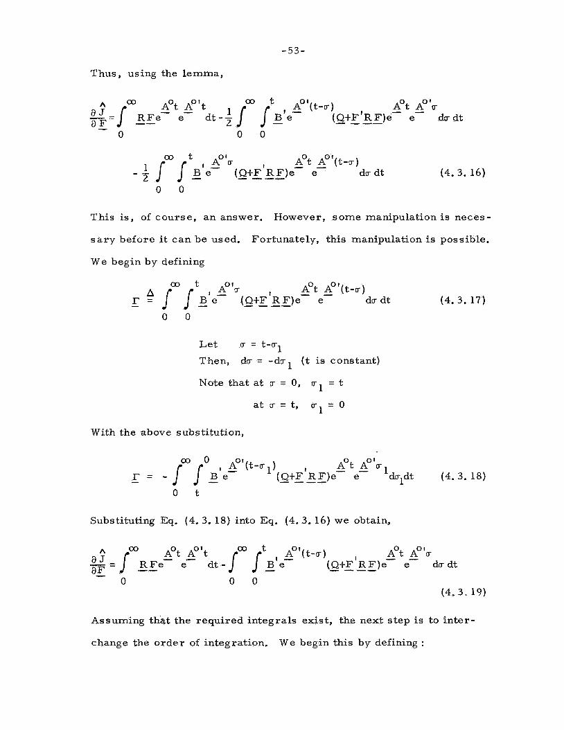
Thus, using the lemma,
Aot A" 'c Ao'(t-r) - - G o t Aot Ao't oo aJ [ -- RFe- e - d t - i / [B'e- - (QtF 'RF)e e dudt a F = 0 0 0
I Ao'r Aot A" ' ( t - IT ) - 1 [ I e- (QtF 'RF)e- - --- e- dcr dt (4.3. 16) 2
0 0
This is, of course, an answer. However, some manipulation is neces-
s a r y before it can be used. Fortunately, this manipulation is possible.
We begin by defining
Aot Ao'(t-r) - - A" 'cr o o t
- r = * [ [ - B'e- ( Q t F ' R F ) e - --- e dcr dt (4.3. 17)
0 0
1 Let cr = t-cr
Then, dr = -dcr (t is constant) 1
Note that a t cr = 0, r1 = t
a t c r = t , u 1 = 0
With the above substitution,
Aot Ao'c Ao'(t-cr 1) 4 -
0 0 0
- r = - I ,I' - Ble- (QtF 'RF)e - --- e dcrldt (4.3. 18)
O t
Substituting Eq. (4. 3.18) into Eg. (4.3.16) we obtain,
Aot A" ' t Ao'(t-cr) - - Aot Ao'r A - a F =JmRFe- -- e d t - / / - B'e- ( Q t F ' R F ) e e du dt - 0 0 0
(4,3. 19)
Assuming that the required integrals exist, the next step is to inter-
change the order of integration. We begin this by defining :

-54-
Ao'( t-rr) - - Aot A" 'cr o o t
(Q tF 'RF)e e d r dt - X = 'I I - B'e- - --- 0 0
Interchanging the order of integration :
Ao'( t-cr ) ,4Ot Ao'cr - X = Sa - B'e- (QtF 'RF)e- e- d td r
(4.3.20)
(4.3.21) o u
Let T = t-cr Then, dT = dt (cr is constant)
Note that at t = 5, T = 0
at t = m , T = C O
With the above substitutions,
AOT A O ~ A O ' ~ - - - AO'T o o o o
x = I - B'e- (QtF 'RF)e - e e dT dcr (4.3.22) - 0 0
Aocr Ao'cr 0 00 AO'T
- X = e B'e- ( rn Q+F'RF')eA --- rdT 1 e- e- d r (4.3.23)
0 0
Substituting Eq. (4. 3.23) into Eq. (4. 3. 19) we obtain:
Aocr Ao'r 0 a Aocr Aotcr AO'T A 00
~ J = R F J a F -- e e dcr - - B' ,"e- (a+F'RF)e' Tdr[ e- e- dcr - -
- 0
A a J a F Setting - -
0 0
= 0, we obtain Ff& -
(4.3.24)
0 (4.3.25)

- 5 5 -
Define :
(4.3.26)
0
Equations (4. 3.25) and (4.3.26) a r e fairly close to the solution
of the problem, assuming that the required integral exists. The fol-
lowing theorem guarantees existence and uniqueness under the assump-
tions that a r e well known to be necessary.
- Theorem 4. 1 Given the linear time-invariant system (4.2. 1)
and the performance criterion (4. 2. 3) and
a ) the matrix [ B, AB, A 2 B, . . . . ,- An- 1 I31 is of rank n e -- - -
( c ontr ollability7 ) I 1 , ( A * ) ~ - ~ H ' J is of rank n, b) the matrix [H', A H , . . . . - - - --
where Q = HIH; ( ~ b s e r v a b i l i t y ~ ) - -- .b
then the constant matrix - F' which minimizes the cost functional
(4. 2. 3) is given by
(4.3.27)
is the unique positive definite solution of either Eqs. (4. 3.26) and K::: -
and (4. 3.25) or, equivalently, of Eq. (4. 3. 28) below :
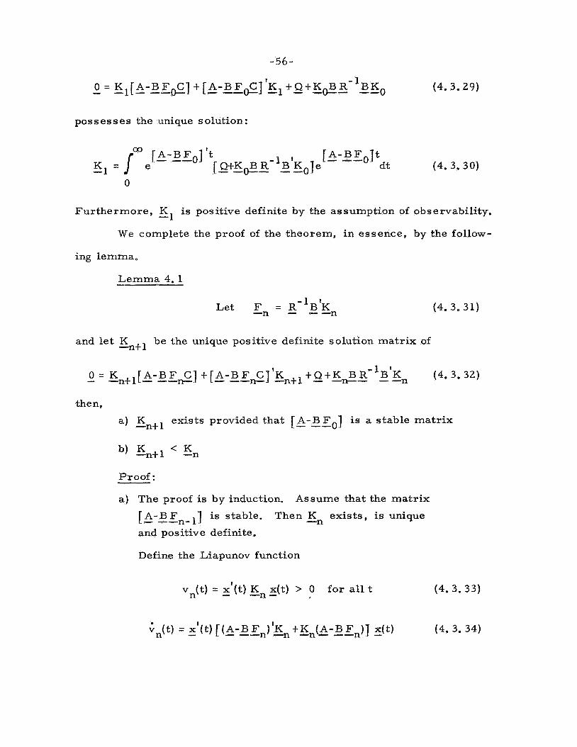
(4.3.28) K:kA + .II - K"B R-lg'K" - --- -- o = - - - -- Proof: Since the system (4.2. 1) is controllable, there exists
a positive definite symmetric n x n matrix KO such that
stabilizes the system (4. 2. 1). Thus, by Theorem 4, p. 231, of
reference [ 181, the equation
possesses the unique solution:
Furthermore, K is positive definite by the assumption of observability.
W e complete the proof of the theorem, in essence, by the follow-
-1
ing lemma,
Lemma 4.1
Let F = R - ~ B ' K -n - - -n (4. 3.31)
and le t EStl be the unique positive definite solution matrix of
0 = K [A-BF D- C 1 + [ A - B F ~ ] ' K n t l t Q t K - -- - -D-- BR-lB'K - -n (4. 3. 32) -n+l - -- -
then,
exists provided that [ - A-B -- Fo] is a stable matrix a) E n t l
Proof:
a ) The proof is by induction. Assume that the matr ix
is stable. Then K exists, is unique [A-BFn- 11 -n and positive definite.
Define the Liapunov function
vn(t) = x'(t) K x(t) > o for all t (4.3.33) -n - -
G n ( t ) = - x'(t) [(A-B - --n F )'K -n t K -n- (A-B --n F )I .- x(t) (4. 3.34)

-57-
Let
V -n n -n -n.--- 4 [ A - B F - -- 1 ' K t K rA-BFnJ (4. 3. 35)
-K ) B R - ~ B ' ( K -K ) -n v = - Q - K - --- B R - ' ~ ' E ~ - ( K ~ - ~ -n -- - -n-1 -n
Therefore V < 0 and Cn( t ) < 0 for all t -n -
(4.3.39)
(4.3.40)
Therefore, [ A - B F - --n-l J is stable implies [A-BFnJ - -- is stable s o that K induction from F -0'
exists and (a) is proven by -nt 1
b) The proof that Xntl< En is obtained as follows :
0 = K A-BR-lB'K --n ]t[A-BR-lB'K _ _ _ ]'K t K BR-lB'K - -n - -n+i- -- --n -ntl -v-

-58-
This equation has a unique negative definite solution for [ K - K 1. . -nt l -n
By the lemma just proven, the sequence of matrices (K 1 is -n
a monotone decreasing sequence of positive definite matrices.
sequence must converge to a positive definite limit - K". be a solution of Eq. (4. 3.28) or , equivalently, of Eqs. (4, 3.25) and
(4. 3. 26).
ulation which may be found on p. 77 , reference [ 1 I].
Such a
This - K* must
Uniqueness follows f rom a straightforward algebraic manip-
This completes the proof of the theorem. And, the theorem
guarantees the existence of the integrals (4. 3. 20) and (4.3. 21) , there-
by completing the derivation of the solution to the Kalman linear
regulator problem.
4.4 The Main Result
In this section we relax the assumption that C = I to the c -
assumption that C is a rea l r x n constant matrix of rank r ( r - < n).
Thus, the results we obtain will apply exactly to the problem stated in
Section 4,2.
cated than those of the previous section.
the structure of the solutions are quite similar.
The results we actually obtain are somewhat more compli-
However, the derivations and
We remark that the
existence of a constant - F which stabilizes the system (4.2, 1) is as -
sumed throughout this section. If such an - F does not exist, then J
is infinite for all allowable controls and our problem is meaningless.
A
We. begin by using Eq. (4.2.2) to rewrite the performance c r i -
terion, Eq. (4.2.3), as

- 5 9 -
Guided by our experience in the previous section, we will again calcu-
late - aF by application of the lemma and example of the previous sec-
tion.
A a J - Again, we define the convenience,
A' e [A-BFC] e - --- (4.4.2)
Then,
J (4.4.3)
Using the example, it is easy to show that, to first order in E ,
c- AO-EB --- AFC] t - Aot - E /" e&0(t-5) A00 BAFCe- dr --- e = e (4.4.4)
0
Applying Eq. (4.4.4) to Eq. (4.4. 3) we obtain, accurate to first order
in E ,
f
A" t - A" 't Aot ( Q t C ' F ' R F - - - --- C)e t 2~ e ( C ' F ' R m - - -- - C)e-
0
A" t (QtCIFIRFC)e- - - d ---
A
- -
--- Ao'(t-cr) ,
--- B AFC e- Aord3} dt (4.4. 5) - A" 't
- € e (QtC 'F 'RFC) - -----

-60-
Then, to first order i n € ,
L 0
Aou - A"% - Ao( t - r ) B dr Ahp -I - Ce- e (QtC 'F 'RFC)e - - - - -
0
(4.4.6) - - I 1'- Ao(t-5) - A"$ - AOr - ~ e - e (QtC 'F 'RFC)e - - - --- B d r A F dt
0
Using Kleinman's lemma,
h Aot A"\ Ao\t-r) 1 1 % Aot Aob o o t
-- aF a J - l m R F C e - --- e- - C'd t -$ j I - B'e- (QtC - ----- F RFC)e- e- - C d r d t - 0 0 0
A0'T Aot - A" ' ( t - u ) o o t -:I 2 I - B'e- (Q+C 'F 'RFC)e - - - --- e - C'drdt (4.4.7)
0 0
This i s nicely parallel to Eq. (4. 3. 16) and it is obvious that the identi-
ca l substitutions wi l l produce s imilar results. Thus,
A" 'r Aot Ao'(t-r) , o o t
Let - I? 5 I E'e- (QtC'F 'RFC)e- - - --- e- - C du d t (4.4.8)
0 0
Let u 1 = t-s
Then, do- = -du (t constant) 1
Note that at r = 0,
at r = t,
r1 = t
r1 = 0
-61-
I\
a J Substituting Eq. (4.4. 13) into Eq. (4.4. 10) and setting - i3F -
With the above substitutions,
= 0 ,
F" -
Ao'(t-s 1 ) - - Aot A0'r o o t
- I? = I - B'e- (g+C 'F 'RFC)e e d r 1 dt (4.4.9) 0 0
The refore,
AOIt-cr) Aot Aob c o t Aot A"\ aJ = JooRFCe- --- e- - C'dt-J J - B'e- i3F (Q+C'FIRF - ----- C)e- e- - C'dr dt 4
0 0 0 (4.4. 10)
Let
Aot AO'IT - - A" I (t - cr ) o o t
x = "J ,f - B'e- (QSC'F'RF C)e e C dv dt (4.4. 11) - 0 0
Interchanging the order of integration, assuming the required integrals
exist,
A" I (t - IT ) - - Aot AO'IT - x = sa - B Y - (QtC 'F 'RF - ----- C)e e - C 'dt dcr (4.4.12)
o s
Let T = t-IT
Then, d-r = dt
Note that at t = IT, T = 0
at t = a, T = co
With the above substitutions,
AO'T A05- Ao'a co
x = - B'e- ( Q t C I F I R F C ) e - ----- e e - Clds (4.4. 13) - 0 0
-62-
0
where
0 LO J (4.4. 14)
(4.4. 35)
For some applsations the form of Eq. ,1.4. 14) may _ e the
most useful. However, we can obtain another form that is quite inter-
esting by defining:
0
00 $: * I A 5 A 5
e dr
(4.4. 16)
(4.4. 17)
0
Assuming that a - - K*, L" and F"' exist such that - A*, as defined .1,
in Eq. (4.4. 15), is stable;
Eqs. (4.4.14), (4.4.16) and (4.4. 17);
assuming - K-r and - L* a r e solutions of .b
then K*, L" and F1' a r e also
solutions of the following algebraic equations :
(4.4. 18)
(4.4.20)
.I.
Note that Eq. (4.4.20) can be used to eliminate - F' from the other two
equations.
tions to the single equation of the previous section, Eq. (4. 3.28).
Furthermore, the existence of - C'l reduces the above equa-

-63-
We remark that it is entirely possible that the above algebraic
equations have solutions that a r e not also solutions of the integral
equations, Eqs, (4.4. 14), (4.4. 16) and (4.4. 17). Furthermore, these
a r e only necessary conditions for a solution. These two caveats wil l
be clarified somewhat by the following lemma which also provides an
algorithm for computing - F''*o .L
Lemma 4.2
(4.4.21)
where K is the solution of : -n
and L i s the solution of: -n- 1
a ) Then, assuming - - Qr 0 and [ A - B F - --,I- 1- CJ stable, a
unique and positive definite K exists. -n
b) Furthermore, assuming there exists a positive defi-
nite L which satisfies Eq. (4.4. 23) , then -n- 1
t r [ K J < t r [ K ] (4.4.24) -n - -n- 1
Proof
a) Existence and uniqueness of sn is a direct consequence of
Theorem 4, p. 231, of reference [ 181.
established for an identical equation, Eqs. (4. 3.29) and (4. 3. 30) , in
the previous section.
Positive definiteness was

-64-
A = 6K -n b) Let K -K -n -n-l
We next attempt to compute 6En.
(4.4.25)
I
- K -n- 1 I- A - B F ---n-2- cJ-CA-BF - --,-2C] g n - 1 (4.4.26)
(4.4.27)
Adding and subtracting K B R-lB'K and formihg perfect squares -n- I-- - -n-1
in exactly the same manner as in the proof of Lemma 3. 1, we obtain
Define
Then,
(4.4.28)
(4.4.29)
(4.4. 3 0 )

-65-
co [ A - B F c]'t I A - B F ' ~ . , ~ J I I e dt (4.4. 31) -n t r [6K -n ] = t r k
0
L
t r [ 6 K -n J = tr[I -n- Lnw1J (4.4.33)
Since L is assumed to be positive definite, it can be factored
uniquely into
-n- 1
@ m' = L (4.4. 34) -n- 1-n- 1 -n- 1
The ref ore,
Equation (4.4. 35) is identical in form to Eq. (3. 1. 17). Thus, applica-
tion of the proof in Chapter I11 which follows Eq. (3. 1. 17) demonstrates
that
t r [ 6 K < 0 (4.4. 36) -n
which completes the proof .
If one can find a stabilizing initial guess for the feedback gain
matrix then the above lemma can be used in a computer algorithm that
is essentially s imilar t o the one used in Chapter 111.
gence is not guaranteed but is likely for well-behaved systems.
conjectured that the solutions of the necessary conditions a r e - not unique.
Furthermore, it is conjectured that convergence will not occur unless
Again, conver-
It is

-66-
the initial guess is "close enough" to optimality.
based on two facts:
This conjecture is
1) The algorithm is basically Newton's method and this type
of behavior is characterist ic of Newton's method.
2 ) The Lyapunov argument of the previous section, when it is
applied to this problem, shows that stability of [ - A-B -- F s ] and exis-
tence of
Il--n+l -n
does not guarantee stability of [A-BF-+lC] unless
F -F 1 1 is "small enough",
4. 5 Examples
We have w o r k e d two examples that a r e of some theoretical
interest. They a r e included below.
Example 1 :
a) The system is described by
0.
x t f i i t x = 0 (4.5. 1)
where f is the feedback gain and x is a scalar, function of time.
This system is identical to :
with
- i(t, 0 ) = [ - A-BfC](P(t, -- - 0) - +( 0 , 0 ) = - I
0 '1 - c = [O
(4.5.2)
The system is controllable and observable.
is given by
The performance criterion
(4. 5.3)

-67 -
with - Q = [: :] The solution, as the reader can verify by substituting into Eqs. (4.4. 18)-
(4.4.20) is :
f:? = (4. 5.4)
minimizes the performance cr i ter ion (4.5. 3 ) constrained by Eq. (4. 5.2).
b) It can be shown, by direct substitution, that
00 h J = 1 2 [ (x2tf2k2)dt
0
M
x(O)=O k( O ) = 1
(4.5.5) x( O ) = 1 &( O)= 0
The f which minimizes Eq. (4. 5.5) subject to the constraint imposed
by Eq. (4.5.1) can be computed by a procedure suggested by Brockett.
We include the calculations to demonstrate the method.
Multiplying Eq. (4.5. 1) by &, we obtain
.. . .2 x x t f x t x x = a
Integrating from 0 to 00, we obtain
00 * 2 1 (I;; t f x t x2)dt = 0
0
The ref ore,
00 00 x d t = - ~ [ ( x 1 2 t x ) 02 ]
(4. 5.6)
(4. 5.7)
(4. 5.8)
0 0
-68-
Multiplying Eq. (4. 5. 1) by ( G t f x ) , we obtain,
(k t f X ) ( H t fk) t (k 4- f x ) x = 0
Integrating from 0 to 00, we see that
00 Jm(; t fx ) ( z t f&)dt t r x k d t t J f x 2 dt = 0
0 0 0
Thus ,
03 1 . 2 2 x d t = - - [ x t f x ) f + x ]
0 0
(4.5.9)
(4.5.10)
(4.5.11)
T he ref ore ,
00 03
2 2.2 1 2 2 2 2 2 . 2 2 (x t f x ) d t = - z [ k t f x ) t x t f x t f x 1 (4.5. 12)
0 0
We assume (as is the case) that the minimizing f produces a stable
system s o that x(m) = ;(GO\ = 0.
Thus, i f x(0) = 1, k(0) = 0 then
00 2 2.2 1 2
2 (x t f x ) d t = z ( l t f ) (4.5.13) 0
And, i f x(0) = 0, k ( 0 ) = 1 then
(4. 5. 14) 2 2.2 1 2 'p 2
0 (X t f x ) d t = z ( l t 2f )
Substituting these results into Eq. (4. 5. 15), we obtain a specific func-
tion for J that is, n

A 2 t 3fL 2 f J ( f ) = (4. 5. 15)
Differentiating this expression, setting the derivative equal to zero
and recognizing that we must choose that f for which the resulting
system is stable gives
f>: = (4.5. 16)
There is a third technique which could be used to solve this
example.
the two sets of initial data.
obtain an expression f o r J in te rms of an integral of these Laplace
One could compute the Laplace transforms of x and k for
Then, Parseval 's theorem can be used to A
transforms.
Kaiser" can be used to evaluate this integral directly.
The integral tables in Appendix F of Newton, Gould and
One thus
arr ives at Eq. (4. 5. 15) and proceeds from there.
Example 2 :
This example is identical to Example 4 of Chapter 111 except
that T = 03 and F"' is constant by hypothesis. The parameters a r e : -
The solution, obtained by substituting into Eqs. (4.4. 18)-(4.4.20) and
solving is : .b
(4. 5. 17) f' = 1. 7
Two reasonable conjectures about the relation between the con- .I-
stant - F* of this chapter and the time-varying F*''(t) of Chapter 111,
when they a r e calculated for identical systems and for cost cr i ter ia
whose only difference is in whether T is infinite o r not, a r e :

-70-
1) F" = the "average" value of - F"(t) computed for
T large. rlr
2) 4 F* = the "steady-state" value of - F'(t) computed
f o r T large. By "steady-state" we mean a con-
stant value of I F'(t) m.aintained f o r a t ime interval
between the two terminal transients, if such a
constant value exists.
&
It should be noted that the above example and Example 4 in Chapter I11
support either hypothesis although the first conjecture is supported
more strongly.

CHAPTER V
CONCLUSIONS
In the previous chapters we have studied two very closely r e -
lated output feedback problems. For the first of these problems, the
linear output feedback control of a linear system with respect to a
quadratic cri terion for a finite interval, we found conditions which the
optimal control must satisfy. In addition, we derived and programmed
a computer algorithm which can be used to compute this optimal con-
trol. The second problem, treated in Chapter IV, is identical to the
f i r s t except that the system is assumed time-invariant as well as lin-
ea r , the interval is semi-infinite and we demand that the feedback
matrix be time-invariant. Necessary conditions that the solution to
this problem must satisfy a r e found. In addition, a number of exam-
ples of both types a r e included.
We believe that these results a r e quite interesting, both theo-
retically and practically. From a practical viewpoint, one can use
these results f o r two purposes :
1) To design linear feedback controls, especially when
the state vector has many more components than the
output vector.
2 ) T o study the cost-effectiveness of changing the
measurements in a linear system. In other words,
one can solve the problems discussed in this thesis
f o r several different candidates for - C, compare
the cost of buying each - C with the performance
obtained by it, and choose the best one.
-7 1 -

-72-
Both of these applications have been illustrated in the examples includ-
ed in the previous chapters.
From a theoretical viewpoint, we believe these results repre - sent a contribution to quadratic optimization problems for linear sys-
tems.
cal control theory and modern control theory.
In addition, these results will help span the gap between classi-
We believe that there a r e many potentially useful extensions of
F o r example, in the classical design of feedback con- this research.
trols it is well known that dynamical compensation is often useful.
Thus, it would probably be useful to extend our results so that they
might be used to calculate "optimal" compensators.
ing question is how does additive noise in the output vector r(t) affect
our results.
of these results in Chapter IV.
is a linear system optimal with respect to the performance c r i te r ia
used in this thesis ?
Another interest-
We have briefly studied still another possible extension
That is the inverse problem ; When

APPENDIX A
ON THE PSEUDO-INVERSE O F A MAT€UX19
The purpose of this appendix is to develop those properties of
the pseudo-inverse of a matrix that a r e relevant to our research.
Since our concern is with matrices we res t r ic t ourselves to the con-
sideration of linear transformations (matr ices) mapping a finite dimen-
sional vector space into a finite dimensional vector space.
these vector spaces a r e defined on the complex field
Al l of
although al l our
results a r e equally true f o r vector spaces on the r ea l field.
closely followed reference 19, Zadeh and Desoer, in this appendix.
We have
With the above comments in mind, we make the following defi-
nitions :
Let 2 be an m-dimensional linear vector space defined on
be an n-dimensional linear vector space defined on
- A be an arbi t rary n x m matrix of complex numbers
Definition A. 1 - The range of a matrix - A i.s the se t %(A) de-
fined by :
X(A) = { y ~ P / y = ~5 fo r Some - X F ~ ) (A. 1)
Definition A. 2 - The null space of a matr ix - A is the se t ;)2 (A)
defined by :
p(A) = I -- A x = 0 ) (A. 2 )
That is, (A) is the s e t of all vectors of x that - A maps into the zero
-73-

-74-
Definition A. 3 - A subspace 8 of a finite dimensional vector
space 2 then for a l l complex numbers a and p, ax t py e&.
is a s e t of vectors of e such that if x and y a r e i n # , - -
Definition A. 4 - Let and 3 be two subspaces of a vector
space . is said to be the direct sum of and 3 , written
9 as x = y t - z where y
I
= 3( i f any - x E may be written in one and only one way
and 2 E 4 . -
Definition A. 5 - Let A be an n x m matrix. The adjoint matrix _I
I A of A is a matrix such that - -
Definition A. 6 - Let 3 be a subspace of e n. The orthogonal
n complement of
that a r e orthogonal to all vectors of
, denoted by @L , is the s e t of a l l vectors of
. Theorem A. 1 - Let A be a matrix in e n; then -
Proof: - Let y 8 (A) (see Definition A. 6 )
Since -- A(Ak) E 6f (A) - and since - y E 4 (A) , we have
0 = <y.A(&x)> = < A 1 ~ , A ' y > = I I A ' y ( I 2 - = 0
Therefore, 4'2 = 0 and y E 7 (A')
1
I
Thus, we have proved that y E (A) I +y E (A') (A. 7)
Let - z € 41 (A') I
then, for all x, 0 = < A z , x > = < z , A x - --- - --

-75-
that is, z is orthogonal to all vectors in (A). Thus, we have proved - z E
Therefore, (11) is proven and 4 (A') =e (A) (I) follows from the fact that e
- (A') ' 5 € 4 (A)' (A. 8)
1
1 = 4 (A) @ 4 (A)
Theorem A. 2 - 1 - A t A is the orthogonal projection of o n t o q ( A ' ) = 4 (A) (A. 14) - -
( A ' ) - + t = - A (A. 15)
- A ~ A A ~ -- = - A+ (A. 16)
(A. 17) A A A = A -I- --- - '1 - A A t is the orthogonal projection of e o n t o 4 (A) =? (A) (A. 18) --
Proof: -- of (I) :
Let - x be an a rb i t ra ry vector i n e Consider the orthogonal decomposition x = x t x where - -1 -2
(A. 19)
Then, A A x = A A x l by the definition of x2 above (A.20)
1 51 € 7 (A) 9 ffz €4 (A)
t - j. --- - - _

-76 -
of (11) :
Next, we verify that - A satisfies the conditions 1-111 of
Definition A. 7 for (A t t ) - a) Let 5 E T ( A v - =((A) by (A. 2 2 ) (A. 24)
(A. 25) 1
then - - x = A y fo r y €7 (A) Therefore A A t x = A A A x = A y from Eq. A. 9 (A. 26) - --- --- But A y = x and condition I is verified - -
then -- A z = - 0 by the line above, thus verifying Condition I1 (A. 27)
c ) Condition I11 is trivially satisfied by - A.
of (III) :
1
(A. 28)
(A. 29) t t 1 By Definition A. 7 , - y1 E 7 (A) A y =
Therefore A t t A(A y) = A A A x1 = A t yl = A t 11 (A. 30) - t t - -- - -- Thereby proving III
of (Iv) :
(11) and (111) imply (IV) trivially

-77 -
Theorem A. - 3 - (A')t = (At)' Proof: ( see Zadeh and Desoer)
(A. 33)
Theorem A. 4 - Let - S be the hermitian positive semi-definite
matrix defined by I
S = A A - -- Then,
(A. 34)
(A. 35)
Proof: ( see Zadeh and Desoer)
Corollary A,2 - Let - A be an n x m matrix, n - > m, of full rank
(rank m). Then,
Proof: By Theorem A. 4 ,
(A. 36)
(A. 3 7 )
But (A'A) -- is a non-singular [ actually positive definite]
m x m symmetric matrix. And, the pseudo-inverse of
an invertible matrix is equal to the inverse ,of the matrix.

APPENDIX B
The computer program used to compute the solutions for the
examples in Chapter ILT is listed on the following pages.
ming language used is the M. I. T. version of For t ran IV for the IBM
System/360 Operating System and the IBM System/360 Model 44 Pro-
gramming System.
The program-
The operation of the program, and of the various subroutines
used, is explained by comment cards preceding each operation. The
data cards needed to provide the program with the input data a r e ex-
plained in comment cards a t the beginning of the listing on the next
page.
-78 -

-79-
/ / R I C C A P I JOB ~ M 4 2 1 9 ~ 3 7 1 9 r 2 t 2 0 0 0 ~ 7 ~ O ~ S R I ~ O ~ ~ * L E V I N E r ~ M S G L E V E L ~ l / /TEST EXEC FORC 9 PARHoC=' EBCDIC .MAP. DECK'
C O O U O I O O O O o o o o e o o o o o o o ~ m O O O a O O O O o e ~ O a o o o ~ o o O o o ~ O O O o ~ o o o ~ e o ~ o o o o ~ m m ~
/ /C.SYSLN DD
C T H I S IS THE MAIN PROGRAM FOR CALCULATION OF THE OPTIMAL OUTPUT C FeEDBdlCK GAINS C C INPUT DATA C NJaoo-d- .oo-ooN LS THE DLMENSLON OF TW STATE VECTOR fPHX I S C M o r o d o J o m ~ 2 o o J M L S THE DIMeNSLON OF THE- CONTROL YECSOR ( F IS I IXLRk C LR%o.oGooo.o-oLR 19 T ENSION OF 7'WE OUTPUT YECTOR C LUl'MAXGo-o 4 0 J I S THE BER OF TIME SAEPS INTO WHICH PHf INTERVAL e IS DLVIBH), HENCE, THE 7ERMINAL T*IME* C I S E E - o J e o - e * - o I S THE NUMBER OF TIMR ST6PS B E T M E N BAOH PRINTOUT C MUXI l 'Somoo-oomIS THE M A X I M U M NUMBER OF TTERATLONS WE WILL TRY C MDREooooooaooo= l SLGNIF IES ADDITIONAL COMPUTATIOMS ARE 10 BE DONE C C THE SECOND DATA CARD SPECIF IES PRINTING FORMATS C THE SECOND.TH1RD AND FOURTH F I E L D S OF A TYPICAL SECOND CARD C FOCLOW C ( ' ' r 2 E l 2 r 3 ) 1 ' ' .4E1203) ( ' ' e €1203) C THE ABOVE CARD IS USEABLE FOR M = ~ ~ H * Z K L R = E ~ C C E PSLOo e o e a o CONVERGENCE OCCURS I F DELTA COST<EPSLO C H o o e e o o o - o e o e o I S THE STEP S I Z E < ' C c - A.B.C.Q*R,SIPHIO ARE READ BY A READ NAHELIST C ~ o o m o o ~ ~ ~ m o o ~ o o ~ o o a ~ a ~ o o a o o a e o o o ~ o ~ o ~ o o o o o o o ~ o o m ~ o o a ~ o o o o o o ~ o ~ ~ o ~ ~
DIAENSION PN(3)rPM(3)rPNN(3)tPMLR13) DLMENSION S 1 2 , 2 ) r Q ( 2 . 2 ) . R ( 2 t 2 ) t P H ~ O ( Z ? Z ) . D U M ( Z . Z ~ ~
1 B T ( 2 ~ 2 ~ . R I B ( 2 ~ 2 ~ ~ P H I ( 2 r 2 ) r P H 1 ~ ~ 2 t 2 ~ ~ F E E D ~ 2 ~ 2 ~ ~ ~ Q ~ 2 ~ 2 ~ ~ C 0 3 T 1 ~ 2 ~ 2 ~ ~ 2 COST242.2)
1 INTMAXvN.HrLR COnMON C K ~ 2 ~ 2 ~ 1 0 0 0 L ~ ~ F 1 2 ~ 2 ~ l O O O l ~ ~ A ~ Z 1 2 ) r B ~ Z 1 2 ) ~
100 RBAD (5.3001 1 Nw He LRe INTMAXt I SEEt M A X I TSI MORE READ ( 5 9 3002 8
READ t 5 r 3003) EPSLOIH
f PN( I b t 131 9 3) r ( PM( J) 9 Jz1 t 3 1 t PNNt K) d K = l , 3 1 e 1 t PMLRtL ) 9 Lx1 r 3 1
C C WE WRITE THE INPUT DATA
WRITE (6140011 INTMAX WRITE 16.4002) EPSLOvH NAnELIST/ZAP/A~BtCtPtR.S.PHIO READ 4 3 r Z A P ) WRI TE ! 6 9 2001 1 WRITE ( 6 r P N ) I I A ( I ~ J ) r J = l r N ) r I ~ L ~ N ) WRITE (6*2002), WRITE (69PM) ( ( B ( I . J ) . J D l . M ) r I I l . N ) WRITE (6.2003) WRITE ( 6 r P N WRITE 1 6 ~ 2 0 0 4 k WRITE ( 6 r P N ) ( ( Q ( I ? J ) . J x l r N ) , I l l r N ) WRITE (6.2005) WRITE ( 6 r P M ) ( ( R ( I ~ J ) . J ~ l r M ) r I ' l r M ) WRITE (6.2006) WRI 1 E ( ( S I I e J 1 Jz1 e N) t 1 =l r N 1 WRITE (6.2007)
t I C ( 1. J) . J z l r N 1 e I *l t LR 1
I 6cPN 1

-80-
C C C
C C
101
C C
L O 2 C C
C c .
103 C C
WRITE ( 6 t P N ) ( ( P H I O ( 1 r J ) r J ~ l r N ) r I " I t N )
FLRST STEP OF COMPUTATIONS
I T$=V
CORlPUTATION OF R-INVERSE BO 101 J S l r M 00 101 I x l r M DUM( 1 rJ1 TR ( 1 J 1 C k L L VECT (DUHrM)
COMPUTATION OF B* 60 102 J= lpH DO 102 I = l r N B P ( J . L ) = B I I r J )
R-INVERS6 TIMES 8-TRANSPOSE IS DEFINED AS R I B c a L MULT t D U N ~ B T ~ R I M* N* HI
WB KNOW AND STORE KtTERMINAL T I M E l = S DO 103 J * l t N DO 103 I q l r N C # ( I ~ J I I N T H A X ) ~ S ( I ~ J ) O W ( I d I = P H I O( f r J 1 PHLT( Jr 11 =PHIO( I J)
P9oc I S USED TO COMPUTE F t O r T J C l l l L PSol.1 (PHI tR IBr INTMAXrFEEDr I~S) 00 104 L * l r I N T M A X 00 104 J w l r L I P DO 104 I W l r M
104 f I r J 9 L ) C Ff ED t I r J B C " C COnPUTATION OF THE COS* I S SET UP
C M L MULT ( P H I O I P H I T ~ S B ~ N ~ N I N ) C l K L MULT l f rS9,COSTl rNrN.N)
C " . ' C R W L BEGINS THE ITERATIVE LOOP. I T CONPUTES K ( N + l r V ) RROM f ( N r T )
C * 105 C l K L RSOL t 9 1 R )
' C ' T H I S IS A CHECK ON THE COklPUTATUIDNS WRITE (6wPN) I ( C K ( I r J r l ) r J ~ l . N ) . I t l t N ~ RRI TE ( 6 s P N I I 4 CK( I. Jr 21) r Jr l r N) 9 I rN1
C C COnPUfltTdON 06 NEW COST
DO 1064 J S l r N QO lo@ I - l r N P H I # I* J 1 *PH IOI I rJ1 COSTPI 1. JBXOoO DO 106 K s l r N
106 C O S T 2 ( I ~ ~ ) ~ C O S T 2 ( I r J ) + C K ( i r K r l ~ * S 9 ~ K r J ) C C T H I S CAUSES THE ITERATION COUNTER TO INCREASE BY lo
C C CHECK FOR CONVERGENCE. ONLY AFTER THE THIRD ITERATION
IT§=ITS+l

-81-
I F ( I T S - 2 1 108r108rl16 116 TR-0-U
DO 107 I r l e N 107 T R s T R ~ ( C O S T l ~ I ~ 1 ~ - C O S T 2 ~ 1 ~ 1 ~ )
I F (TR-EPSLO) 110.110~l08 C C SF COlVERGENCEe IDONE=2 AND WE PRINT DATA. I F NOT, 100 €11 AND PROCEED
168 DO 109 1-l.N 109 C O S T L t I ~ I ~ ~ C O b T 2 l I r l ~
A X I T S I 113r110,110 110 10[3N6*2
WRITE I6r4003) T R e I T S WRITE (6r4004) I S E E WRITE f 6 r Z 0 0 8 1 00 111 L * l r I N Y M A X e I S E E We1 TE f 6 t 2009 1.
I T E 86~2010)
fTP 16,20091
R I T E ( 6 r 2 0 L l C
111 WRITE (6,PNN) I ( C K ( K , J I L ) r J = l r N ) r r a l * N ~
0 112 L * l r INTHAXt ISEE
TE (6 rPMLR1 ( ( F ( I r J , L ) r J = l r L R 1 w I = l , M ~
C C , L l ~ . C A L ~ E ~ TO C O ~ ~ ~ T E F ~ N , T ~ AND P ~ I ~ ~ , T 9 G I V
C C LREADY DETERMINED NCE AND USED THIS YO 5 C GENC€, CHECK FOR IF NOTI REITERATE-
L PSOL ~ P H I ~ R I ~ ~ I D O ~ E ~ ~ S E E ~ I T S ~ P N N ~
GO TO ( 1 0 5 ~ 1 1 4 ) ~ I D O N E l t 4 IP ( N ~ R E a 115plS5e100
3001 FORMAT (716) 3002 FORMAT ( 3 A 4 * 3 A 4 , 3 A 4 , ~ A 4 ~
2001 C'3RMAT t e O T M A-MATRIX IS PRINTED 6ELOWEt 2002 MA^ ( ' 0 THE 6-MATRLX I S PRINTED 6€&.0Wa1
2004 FORMA? ( ' 0 T W Q-MATRIX I S PRINTED 0ELOW'b 2005 PDRHA? ( ' 0 THE R-MATRIX I S PRINTED 6ELOW') 2006 CORMaT ( 0 0 THE S-MATRLX I S PRINTED 86LOW"I 2007 FORMAT f @ Q THE I N I T I A L CQNOITION MATRIX I S PRINTED BELOWa) LO08 FORMllY ( e 0 THE K-MATRIX IS PRINTED BELOUeI 2009 FORMAO ( ' 0 " ) 20k0 FORMAT ( ' 0 THE FEEDB4CK MATRIX IS PRINTED 6 E t O W e t hdll FORMAT ( ' 0 THE TRANSITION MATRIX I S PRINTED 8 E L O W ) 4001 PORMAF ( ' 0 THE INTERVAL IS OIVIOEO INTO ' r 1 4 r ' PARTS' l 4002 FORMAT ( ' 0 CONVERGENCE OCCURS I F DELTA COST I S LE9S THAN r ~ E 1 1 . 4 ,
6003 FORMAT ('I3 DELTA COST I S = ' r E l l e 4 e @ T H I S IS I T E R A T I O N ' r l 4 ) 4004 FORMkr ( ' 0 THE OUTPUT MATRICES ARE PRINTED ONLY AT T*'*14w0*H' 1
C ~~~rrr..rr~.r..rr.rr.~~rr**~..a.rar.a.~~~~**ar~~arr.*.oa~r.~.or~~r.
C SUBROUTINE RSOL
3003 ffORMAT IZE11-4)
2003 PORNAT 1.0 THE C-MATRIX IS PRINTED m.onR)
1 THE STEP 91ZE I S ~ ' p E l 1 * 4 )
l k 5 E M I
C C PURPOSE C TO COMPUTE K f N + l r T D v GIVEN F t N + l r T ) C

- 8 2 -
' C COHMENT C INPUT DATA IS PARTLY TRANSIERRED THROUGH COMMON
G C ~ . o ~ o r o o o . o . r . . o . ~ o . . o o ~ o ~ o o o o o o o o ~ o . o ~ ~ o ~ o o ~ ~ o o o * o o o o * ~ o o ~ ~ * o . o . o
SUBROUTINE RSQL f XQr XR J OWENSION X ~ ~ 2 r 2 ~ r X R ~ 2 t 2 l ~ X D U M ~ 2 r ~ ~ r F C I 2 t 2 l r B F C 4 2 ~ 2 ~ ~ R ~ C ~ 2 t 2 ~ r
COMHON R W ~ 2 r 2 r 1 0 ~ O l ~ r X t ~ 2 r 2 ~ l O O O l ~ r X A ~ 2 ~ 2 ~ r X B ~ 2 r 2 ~ t X C I ~ r 2 ~ r H ~ 1 C F R F C ( 2 ~ 2 ) r A B F t ( 2 ~ 2 ) u X A B F C t 2 i 2 t ~ D # 2 ~ 2 t 4 1
1 LNTMlX.NtMrLR ' C
' 100 N D f L I + I N T H A X * c ' C FIJtST STEP OF RUNGE-KUXTA ROUTINE BEGINS
C COMPUTATION BBGINS AT T=INTMAXt THE TERMINAL TIME
101 DO 102 J * l r N BO 1 0 2 1-l.N
102 X O U M l I r J ) ~ R K l L r J . N D E L T ) C
C L=O
DO 103 JS1.N 00 103 I * l * M FC'I I r J J = O o O
. DO 103 K t l r L R 1 0 3 PC4 I ~ J ) = C C ( I ~ J ) * X F ( I V K . N D E L T ) * X C I K ~ J )
C C W L MULT f XBrFCtBFCrNrNrM) G k L L MULT (XR&C*RFC,MrNrM)
DO 105 J-1.N
C F R F C ( I r J ) = O - O DO l0Ii K f l r M
A W C ( I r J)=XA( I r J I -BFC ( 1 r J)
C
oa i o 5 1 - 1 , ~
104 C F R F C t I * J ) = C F R F C t I r J ) + F t ( K , I ) * R F C ( K r J I 105
C
C
C C EVALUATION OF THE PARTIAL SLOPE I N RUNG€ KUTTA ROUTINE
106 L+L+L
CM.L MULT (XDUMIABFC~XABFC~N~NIN)
DO 107 J S l r N DO 107 I x l t N
107 D ( I ~ J , L ) ~ H * ( X A B F C ( I ~ J ) + X A B F C ~ J ~ ~ ) + X Q ( I ~ J ) * C F R F C ( I t J ~ ~ C C LOGIC FOR ROUTING TO EACH PHASE OF ONE RUNGE KUTTA STEP
C GO TO ~ 1 0 8 ~ l O B r 1 1 0 ~ 1 1 Z ~ t L
108 oa i o9 J * L ~ N DO 109 I I l r N
109 X W J H ( I ~ J ) = ~ ~ * D ( I T J ~ L ) + R K ( I ~ J ~ N D E L T I C
C GO TO 106
110 00 111 JZ1.N DO 111 I - l r N
11 1 X D U M t I t J )=D ( I 9 J I L )+RK ( I 9 Jr NDELT )

- 8 3 -
C
C C
112
113
00 TO 106
C&LCULATfON OF K l N + l t l - l ) DO 113 J f l t N DO 113 I s l r N RK( I r JVNDELT-1 )=RK( I t J r N D E L I ) + ( D ( I , J r l ) + Z e * D ( I t Jr2)+2.*D( t r JT 3 )
1 + D ( I t J t 4 ) ) / 6 . C C TLME I S STEPPED BACKWARDS ONE STEP
C C I F T I S NOT ZERO* WE BEGIN ?HE NEXT S l E P - I F TsOt U€ RETURN TO C M I Ne
C
N Q f LTENDELT- 1
IF (NDELT-1) f14r114r101
114 RETURN
C C C C C C C C C C
C C
C c C C C t
IDONE =2 MEANS THE ITERATIONS HAVE CONVERGED AND COMPUTE THE OPTIMAL P H I - WE DO NOT RECOMPUTE Fe COHPUtE A NEW F AND A NEW PHIe
100 GO TO 4 102r 1061 r IDONE C C THIS ENfRY I S USED TO COMPUTE THE I N I T I A L F-
C C COMPUTATION OF C TIMES P H I
C C COMPUTATION OF C TIMES P H I TRANSPOSE
EMTRY P S O L l I YPHI YR I BINDELY~YFEED~NSTART 1
102 C h L L MULT Y C ~ Y P H I I C P H I ~ L R t N T N l
00 103 J S l r N DO 103 I s l r L R
103 P H I C ( J * I ) = C P H I ( I r J ) C

-84-
C COHPUTATION OF C*PHI*PHI '*C* C k L L MULT ( f P H I t P H I C t C P P C r L R t L R I N )
C C
C C
104
C C 6 C
C C
112
105 C C
1 Q6
101 C
C
107 C C C
C C
109
1 1 3
C C
C 210
108 C
COMPUTATION OF NC*PHI *PHI * *C* ) INVERSE C&L VECf f C P P C r L R I
E X . ETC. C M L MULT (PHICrCPPCrDUMlrNrLRrLR) ClsKL MULT ( Y P H I ~DUM~~DUMZIYILRTN) DO 104 J s l r L R DO 104 I z l r N DUM31 IrJIxOiO DO 104 K f l t N B U H 3 ( I t J ) ~ D U M 3 ( I t J ) + P K ( I r K r N D E L T ) * D U M Z ( K t J ) C&L L MULT ( YR I B r DUM3 r YFE ED t Me L R t N 1
V'FEED IS NOW THE VALUE OF F AT T H I S TSME AND T H l S ITERATlON
W 8 CONTINUE IF NSTARTrOt THIS IS F t O r T ) AND WE RETURN TO MAIN. I F NSTART 0.
I F (NSTART) 114t114r112
T H l S STORES THE NEW VALUE OF F I N THE PROPER PLACE DO 109 J ' l r L R DO 105 I * l * M YF
KNOWING F 7 WE BEGIN COMPUTING THE VALUE O f PHI AT THE NEXT TIME 00 1 0 2 J x l r N DO 101 I = l , M FOt 1 9 J1=0-0 BO 101 K I l r L R F C ( I r J ) t f C ( I ~ J ) * Y F ( S t K t N D E L T ) * Y t l K I J )
GkLL MULT ( Y B t F C r B F C t NrNrM)
BO 107 J I l r N DQ 107 I t l t N A ~ C ( I t J ) = Y A ( I , J ) - B F C ( I I J l
I t .Jt NDE L T 1 rYFEEO ( I r J 1
IF I D O N E = l t WE S K I P THE WRITING ROUTINE- I F IDONE=2t WE URITE EVERY I C E VALUES OF P H I GO TO 1 2 L O t 1 0 9 ) t SDONE
ROUTINE FOR WRITXNG P H I ICE= ICE + 1 I F (ICE-!SEE) 210 t l l 3 r113 ICE=O WRITE t 6,10001 WRI TE 4 6 PNN 1 t ( Y PH I ( I 9 J 1 t J= 1 r N t L= 1 t H
CONTINUATION 3 F THE COMPUTAJIDN OF CACL MULT (ABFC~YPHIIABFCYININ~N)
DO LOB J P l r N DO 108 Is1.N YPHI(I~Jl*YPHI(IrJ)+H*ABFCY(~~J)
NEXT P H I

-85 -
C C Ye STEP THE TEME ONE STEP
C C I F WE HAVE REACHED THE TERMINAL TIME* WE RETURN TO MAIN0
110 NOELT-NDELT+l
IF (MbELT-INTXAX) l O O t 1 1 1 t l l l 111 I F t I 0 O N E - 2 ) 1 1 4 t 1 1 5 e 1 1 4 lT5 WRITE (6r1000)
Y R I TE I 6 r P N N ) ( (YPH I f I t J 1, J = l r N ) t 1 x 1 t N) 114 RBTURN
C C D m U G PACKET PRINTS USEFUL D4TA
DeBUG SUBTRACEtINITIYRIBtIDONE)
I F (NUELT-1) 300r300r301 AT 112
300 DWPLAV D W 3 r D U M 2 t D U M l rCPPCrCPH1 TFC 301 COPJTIYUE
EM) C C ~o..eoo.~o~.o~.~~..~oooeoeeooeo*.o..eooe.eeo.oo.eeoeea~ooeoooo.oeo
C 0 . . o * ~ e o e ~ ~ ~ ~ . . ~ . e o ~ . e ~ e e . e . o o a . e o o o e o e o o e e e ~ e e e ~ o o o e o ~ . . a o e e e e e e o
C C SUBROUTINE MULT C C PURPOSE C TO COMPUTE THE PRODUCT OF TWO MATRICES- C ' GAMMAIN X M ) = ALPHAlN X L ) * BETAtL. X M ) C C USAGE C CALL HULTfALPHA*BETApGAMMA,NtM,L) C C DESCRIPTION Of PARAMETERS C ALPHA- N X L REAL MATRIX C BETA - L X M REAL MATRIX G GAMMA- N X M REAL MATRIX C N - NUMBER OF ROWS I N ALPHA C M - NUMBER OF COLUMNS I N BETA C L - NUMBER OF COLUMNS(R0WS) I N ALPHA(8ETA) C C 4 . . ~ o 0 ~ 0 r . ~ ~ ~ . ~ 0 ~ r . . . 0 . 0 0 ~ . 0 ~ . e 0 0 0 0 . . e e . 0 e e 0 e a 0 a 0 e 0 0 4 ~ 0 ~ e 0 ~ 0 . 0 0 . 0 e e
C SUBROUTINE MULT(ALPHAe6ETAtGAMNAtNTMtL) OWENSION ALPHAI2t2)rBETA(2rZ)tGAMMA(Z,Z) DO 10 I l l t N 00 10 JX1 .M GknMAt I t J ) = O e O BO 10 K Z l r L G ~ M A ( I ~ ~ ~ ' G A ~ M A l I ~ J ) + A L P H A ( I ~ K ) * B E T A ~ K t J )
10 C W T f Y U E RETURN E NO
C 0. . a ~ a ~ . ~ . o . ~ o o . . . ~ e o . e o e o e ~ e o e o e e a . . . e e o o ~ r o ~ e ~ e o o e o e ~ e a o e o e ~ ~ e o o
C C $I_IRRQIJRT MF V F f 1 C C PURPOSE

-86-
C TO CONVERT A SQUARE MATRIX TO VECTOR MDDE=O* C TO CALL THE MATRIX INVERSION SUBROUTINE AND C TO RECONVERT THE INUERTEO VECTOR TO MATRIX FORM. C C USAGE C CALL VECT (RMATI M 1 C C ObSCRIPTION OF PARAMETERS C M - THE DIMENSION OF THE SQUARE MATRIX C RMAT - THE MATRIX TO BE INVERTED AND I T S INVERSE C C RRMARKS C THE INVERSE IS STORED I N THE LOCATIONS OF THE INPUT MATRIX. C C SUBROUT I N E S REQUIRED C INVERT C C .................................................................. C
SUBROUXIYE VECT(RMAT*M) DLMENSION R M A F ( Z r Z l r A M A T ( 4 )
C MdlTRIX TO VECTOR CONVERSION JNOT*CY
150 JHOT=JNOT+l 1FfM.LT.JNOTIGO TO 180 KONErl+M*( JNOT-1)
00 176 K=KONE,KEND I-K-H+t JNOT-1) AMAT(K)=RMAT(IsJNOT)
KEN D= M* J NOT
170 CCINTINUE
180 CONTINUE GO TO 150
C W T R I X I N V E R S l ON
C VSCTOR TO MATRiX CONVERSION C#L L L NVER T t AHAT * M * M 1
ICNOT=M*H 00 190 K = l t K N O T J=( K-1 )/M+1 I*K-M*t J-1) RWATt I t J )=AMA?( K )
190 CONTINUE RETURN E no
C C .................................................................. C .................................................................. C t SUBROUT I NE INVERT C C PURPOSE C TO INVERT A REAL SQUARE MATRIX C C USAGE C CALL I N V E R l t A * N N v N ) C C DeSCRIPTION OF PARAMETERS

-87-
C A - REAL: SQUARE NATRIX T O BE INVERTED C NN - ORDER OF MATRIX A C N - MAXIMUM ORDER OF A. SET EQUAL TO NNe C C NRTHOO C THE INVERSE OF A I S COMPUTED AND STORED I N A o C C RBMARRS C THLS SUBROUTINE I S A S L I G H l L Y MODIFIED VERION OF 7 N 0 IEM SHARE NO- 1533 MATRIX INVERSION SUBROUTINE. C C ~Ll..r..rr...r..r...~.~...rr.o...*..oo*~.*.m***..ao*oao
C SUBRBUPINE INVERT( A9NN.N) DEMENSION A (41 t Mc 2 B t C ( 2 ) IF(NNeNEo1)GO TO 80 A t 1 B * l o / A ( 1) GO TO 300
80 DO 90 I x l r N N
90 CONTINUE wf I )=-I
DO 140 I - l t N N
@+Or 0 BO 112 L t l r N N l F # M ( L ) * G T o O ) Q O TO 112 J *L DO 110 K r l r N N 1 F t M f K ) r G T - O ) G O T O 108 I F ( A 6 S ( D ) - A B S ( A ( J I ) ~ 1 0 5 ~ ~ 0 5 ~ 1 0 8
C LOCATE LARGEST ELEMENT
105 LO=L KOIK 0 9 A 4 J )
108 J*J+N 110 CONTINUE 112 CONTINUE
C INTERCHANGE ROWS TEMP*-N t LD 1 M( L D I =Hc K D ) #( ICD) -TEMP
L4.D K*KD DO 114 J s l r N N C4 J) * A t L 1 A ( L ) = A (Io A(l(r)*C( J) L+L+N
114 KJ(+N C DLVIDE COLUMN BY LARGEST ELEMENT
N R P t K O - l I * N + l NH*NR+N-L BO 119 K t N R t N H
115 A I K ) * b f K ) / D C REDUCE REMAINING ROWS AND COLUMNS

-88 -
L=1 00 135 J z l r N N IF(J -NEoKD)GO TO 130 L=L+N GO TO 135
A I L ) = A ( L )-C1 J)*Af K) 130 DO 134 K+NR*NH
134 L 4 + 1 135 CONTI'YUE
C REDUCE ROW C t K D ) * - l o O J=UD DO 140 K+l,NN A t J J S-C ( K B /D J* J +N
140 CONTINUE C INTERCHANGE COLUMNS
DO 200 I * l r N N L=O
L F ( H l L ) e N E - I ) G O TO 150 150 LWL+l
K*dL -L ) *N* l J=( 1-1 )*N+1 R ( L l = M l I ) Ml I ) = I
TEMP-AI K 1 A ( los4f J) AlJ )=TEMP J = d + l
200 K*K+l 300 CONTINUE
RRTURN ENO
DO 200 L t l r N N
C C 0 . 0 . . 0 ~ . . 0 0 0 0 . . . . . 0 0 0 0 0 . 0 . 0 0 0 . ~ 0 0 0 0 0 0 . . ~ 0 0 0 0 . 0 ~ 0 . 0 0 0 * 0 0 0 0 ~ * ~ 0 0 0 0 ~ ~
/*

REFEI ?.VJCES
1. Nyquist, H., "Regeneration Theory, Bell System Tech. J . , 11, pp. 126-147 (1932)
2. Hazen, H. L., "Theory of Servomechanisms, I t J. Franklin Inst., 218, pp. 543-580 (1934)
3. Wiener, N. , The Extrapolation, Interpolation and Smoothing of Stationary Time Series, Technology Press, M. I. T. , Cambridge, Mass., 1949
4. Athans, M. and Falb, P. F. , Optimal Control: An Introduction to the Theory and its Applications, McGraw-Hill Book Go., New York, 1966
5.
6.
7 .
8.
9.
10.
11.
12.
13.
Kalman, R. E., "Contribution to the Theory of Optimal Control, Bol. SOC. Mat. Mexico, pp. 102-119 (1960)
Kalman, R. E . , "When is a Linear System Optimal?, J. Basic Engineering, (ASME Trans. ) Vol. 86, pp. 1-10 (1964)
Kalman, Ho, and Narendra, "Controllability of Linear Dynamical Systems, Contributions to Differential Equations, Vol. 1, 1962
Kalman, R. E. , "Mathematical Description of Linear Dynamical Systems, J. SIAM on Control, Ser. A . , Vol. 1, No. 2, pp. 152- 19.2 (1963)
Kalman, R. E. and Bucy, R. S. , "New Results in Linear Filtering and Prediction Theory, J. Basic Engineering, (ASME Trans. ), Vol. 83, pp. 95-108, March, 1961
Luenberger, D. G., "Observers for Multivariable Systems, IEEE Trans. on Automatic Control, Vol. AC- 11, pp. 190- 197, April, 1966
Kleinman, D. L., "On the Linear Regulator Problem and the Matrix Riccati Equation, I ' Electronic Sys terns Laboratory Report 271, Mass. Inst. of Tech., (1966)
Athans, M. , "The Matrix Minimum Principle, Information and Control, Vol. 11, pp. 592-606, Nov. -Dec. (1967)
Kleinman, D. L. and Athans, M., "The Design of Suboptimal Linear Time -Varying Sys terns, trol , Vol. AC-13, pp. 150-159, April (1968)
IEEE T rans . on Adtomatic Con-
-89-
-90-
REFERENCES (Contd. )
14.
15.
16.
17.
18.
19.
20.
21.
22.
Kleinman, D. L., Fortmann, T . , and Athans, M., "On the Design of Linear Systems with Piecewise Constant Feedback Gains, Preprints of Ninth Joint Automatic Control Conference, pp. 698- 7 10, June ( 1968)
Kleinman, D. L., "Suboptimal Design of Linear Regulator Systems Subject to Computer Storage Limitations, ' I Electronic Sys tems Laboratory Report 297, Mass. Inst. of Tech., (1967)
Brockett, R. W. and Lee, H. B. , "Frequency-Domain Instability Criteria for Time-Varying and Nonlinear Systems, Proceedings of the IEEE, Vol. 55, No. 5, pp. 604-619, May (1967)
Luenberger, D. G., "A New Derivation of the Quadratic Loss Con- t ro l Equation, " IEEE Transactions on Automatic Control, Vol. AC-10, No. 2, p. 202, April (1965)
Bellman, R. , Introduction to Matrix Analysis, McGraw-Hill Book Co. , New York ( 1960)
Zadeh, L. A. and Desoer, C. A., Linear Systems Theory, McGraw- Hill Book Co., New York (1963)
Roxin, E. , "The Existence of Optimal Controls, I t Michigan Math. J . , 9, pp. 109-119 (1962)
Filippov, A. F., "On Certain Questions in the Theory of Optimal , Control,' ' J. SIAM on Control, Ser. A, Vol. 1, No. 1, pp. 76-84 (1962)
Newton, G. C., Gould, L. A, , and K a i s e r , J. F. , Analytical Design of Linear Feedback Controls, John Wiley and Sons Inc. , New York, 1961 -
23. W i l l i s , B. H., "On the Least-Squares Optimization of Constant Linear Regulator Systems, Ph. D. thesis, Dept. of Aeronautics and Astronautics, M. I. T . , September, 1965
24. Ferguson, J. D. and Rekasius, Z. V., "Optimal Linear Systems with Incomplete State Measurements, Proceedings Sixth Annual Allerton Conference on Circuit and Systems Theory, pp. 67 1-679, October (1968)
25. Rekasius, Z . V., "Optimal Linear Regulators with Incomplete State Feedback, Vol. AC-:2, pp. 296-299, June, 1967.
IEEE Transactions on Automatic Control,