Embed Size (px)
Citation preview

Optimal PEEP settings in Mechanical Ventilation using EIT
by
Ravi Baldev Govindgi Bhanabhai, B.Eng, Ryerson University
A thesis submitted to the
Faculty of Graduate Studies and Postdoctoral Affairs
in partial fulfillment of the requirements for the degree of
Master of Applied Science in Electrical and Computer Engineering
Ottawa-Carleton Institute for Electrical and Computer Engineering
Department of Systems and Computer Engineering
Carleton University
Ottawa, Ontario, Canada, K1S 5B6
(c) Copyright 2012
Ravi B. G. Bhanabhai, April 2012

Library and Archives Canada
Published Heritage Branch
Bibliotheque et Archives Canada
Direction du Patrimoine de I'edition
395 Wellington Street Ottawa ON K1A0N4 Canada
395, rue Wellington Ottawa ON K1A 0N4 Canada
Your file Votre reference
ISBN: 978-0-494-91577-6
Our file Notre reference
ISBN: 978-0-494-91577-6
NOTICE:
The author has granted a nonexclusive license allowing Library and Archives Canada to reproduce, publish, archive, preserve, conserve, communicate to the public by telecommunication or on the Internet, loan, distrbute and sell theses worldwide, for commercial or noncommercial purposes, in microform, paper, electronic and/or any other formats.
AVIS:
L'auteur a accorde une licence non exclusive permettant a la Bibliotheque et Archives Canada de reproduire, publier, archiver, sauvegarder, conserver, transmettre au public par telecommunication ou par I'lnternet, preter, distribuer et vendre des theses partout dans le monde, a des fins commerciales ou autres, sur support microforme, papier, electronique et/ou autres formats.
The author retains copyright ownership and moral rights in this thesis. Neither the thesis nor substantial extracts from it may be printed or otherwise reproduced without the author's permission.
L'auteur conserve la propriete du droit d'auteur et des droits moraux qui protege cette these. Ni la these ni des extraits substantiels de celle-ci ne doivent etre imprimes ou autrement reproduits sans son autorisation.
In compliance with the Canadian Privacy Act some supporting forms may have been removed from this thesis.
While these forms may be included in the document page count, their removal does not represent any loss of content from the thesis.
Conformement a la loi canadienne sur la protection de la vie privee, quelques formulaires secondaires ont ete enleves de cette these.
Bien que ces formulaires aient inclus dans la pagination, il n'y aura aucun contenu manquant.
Canada

Abstract
Ventilator Induced Lung Injury (VILI) is a serious condition caused by sub-optimal
settings of mechanical ventilation in Acute Lung Injury (ALI) patients. The main con
tributors to VILI are 1) cyclic opening and closing of collapsed lung tissue which occur
at low pressure and 2) overdistension of lung tissue which occur at high pressures. The
key clinical measure to reduce VILI is selecting an appropriate Positive-End Expira
tory Pressure (PEEP) to make a balance between keeping lung units open while not
overdistending them. Electrical Impedance Tomography (EIT) provides regional lung
air volume information which promises to help improve clinical selection of PEEP.
The goal of this thesis is to develop automated methods to analyse EIT data to select
a PEEP value. A novel algorithm is proposed to: 1) locate regional inflection points
(IP) using a linear spline method and 2) to classify lung tissue as Collapsed, Nor
mal, or Overdistened using a Fuzzy Logic System and to suggest an Optimal PEEP.
These algorithms were implemented, tested, and compared to previously suggested
approaches, using a clinical database of ALI and healthy lung patients.
iii

Acknowledgments
I would like to take this opportunity to to thank my supervisor, Dr. Andy Adler,
whose guidance and extensive knowledge made this thesis possible and an excellent
experience. I would also like to acknowledge his interests in computer systems in which
he provided us with excellent equipment to perform our calculations. In particular the
server provided that had the following specifications: Intel Corporation 5520 chipset,
16 Intel Corporation Xeon 5500 processors running at 2.67GHz with 4 cores and 8MB
of cache in each processor, and 64GB of RAM. Working on his sever was a real fun
experience.I would also like to acknowledge my colleagues whose advice, friendship,
and intellectual conversations helped me progress through my masters. Without their
help and companionship the long hours within the lab would not have been possible.
In addition to my colleagues I would like to extend a thank you to the Systems and
Computer Engineering Technical Department and Administrative staff. Their help
with my computer issues and paper work helped save invaluable time.
Lastly, I would like to thank my family. Words can not say how much help they
have provided me throughout my career at Carleton University. Their presence alone
helped me get through the darkest times of my masters. To them I raise a glass.
iv

To my family,
were always there during
the lows and the highs

Contents
Front Matter iii
Abstract iii
Acknowledgments iv
Dedication v
Contents vi
List of Figures x
List of Tables xv
List of Acronyms & Terminology xvii
I Background 1
1 Introduction 2
1.1 Thesis Objective 3
1.2 Thesis Contributions 3
2 Lung Injury 5
2.1 Acute Lung Injury 6
2.2 Ventilated Induced Lung Injury 7
2.3 Pressure - Volume Curves 8
vi
CONTENTS vii
2.3.1 Models of Respiratory Function 9
3 Electrical Impedance Tomography 12
3.1 EIT in Mechanical Ventilation 13
4 Data and EIT Reconstruction 16
4.1 Data 16
4.1.1 Patients 17
4.1.2 Pressure Maneuver 17
4.2 EIT Reconstruction 18
4.2.1 Forward Model 22
4.2.2 Reconstruction Model Used 23
4.2.3 Data pre-analysis 23
5 Fuzzy Logic 27
5.1 Fuzzifier 29
5.1.1 Fuzzy Sets 29
5.1.2 Membership Functions 31
5.2 Inference 32
5.3 Defuzzifier 32
5.3.1 Centroid Method 33
5.3.2 Center-of-Sums 33
5.3.3 Height Defuzzifier 33
5.3.4 Center-of-Sets 34
II Contributions 35
6 Inflection Points 36

CONTENTS viii
6.1 What are Inflection Points 37
6.2 Importance of Inflection Points 37
6.3 Techniques to Locate Inflection Points 40
6.3.1 Visual Heuristics 40
6.3.2 Sigmoid Function 41
6.3.3 Three - Piece Linear Spline 43
6.4 Results 44
6.5 Summary and Discussion 44
7 Algorithm Design 47
7.1 Inflection Point Calculation 50
7.2 Fuzzification 51
7.3 Premise Calculation 53
7.4 Defuzzification 54
7.5 Summary and Discussion 55
8 Results and Analysis 57
8.1 Inflection Points 57
8.1.1 Inflection Points for Individual Algorithms 57
8.1.2 Linear Spline vs. Sigmoid Method 58
8.1.3 Linear and Sigmoid vs. Visual Heuristics 63
8.1.4 Conclusion 66
8.2 Membership Graph and IF-THEN Rules 67
8.3 Optimal PEEP 68
8.4 Conclusion 71
9 Summary and Future Work 77

CONTENTS ix
9.1 Future Work 78
9.1.1 Lineax Spline Improvements 78
9.1.2 Fuzzy Logic Improvements 79
9.1.3 Future Testing 80
A MATLAB Code 82
A.l Linear Spline 82
A. 1.1 Bin function needed for Spline 85
B Results Extra 89
B.l Human vs. Linear Table 89
B.2 Visual Heuristics Pixel Locations 90
References 91

List of Figures
2.1 An example of a pressure-volume and pressure-impedance curve for
both inflation and deflation limbs. From these curves inflection points
can be found to be used within guided ventilation strategies. For more
information on inflection points refer to Chapter 6
4.1 Pressure, Volume, and Flow of the recruitment maneuver performed.
Only the ramp regions, as segmented between the two lines was used for
this study. The data before and after the black lines are of ventilation
of the patient
4.2 Location of the plane where the electrodes are placed equally-
spaced around the patient, 5th intercostal plane. Reproduced from
[Rawlins et al., 2003]
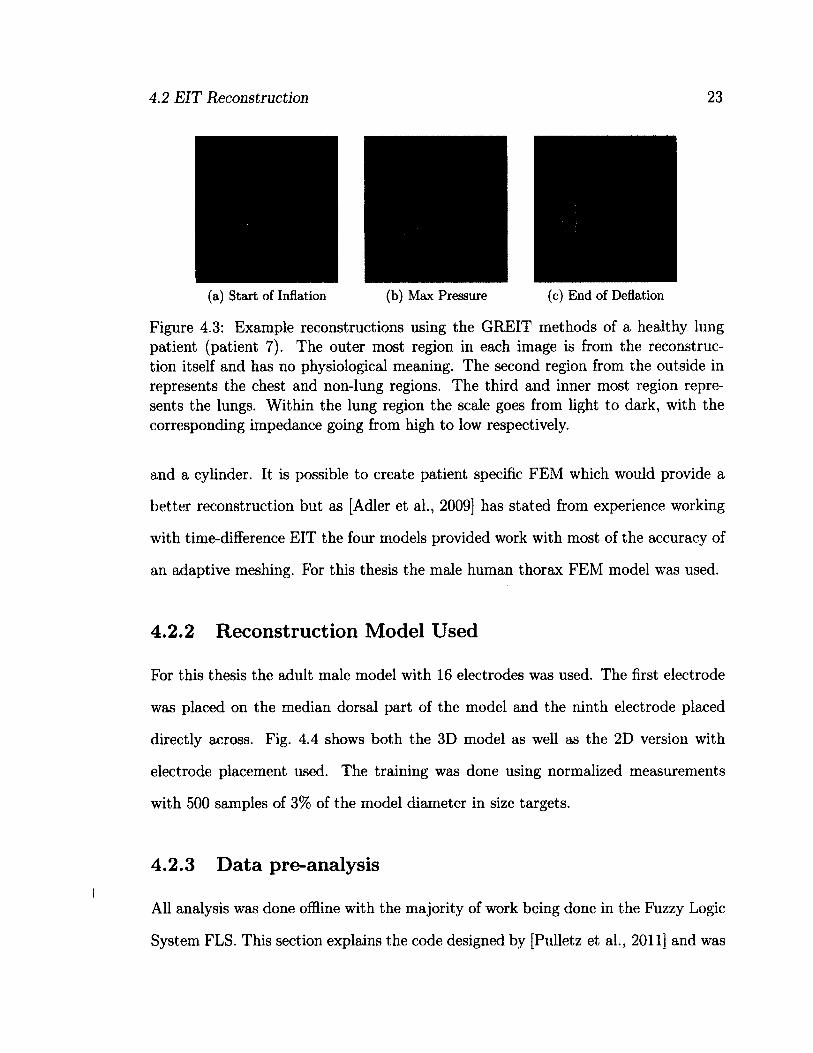
4.3 Example reconstructions using the GREIT methods of a healthy lung
patient (patient 7). The outer most region in each image is from the
reconstruction itself and has no physiological meaning. The second
region from the outside in represents the chest and non-lung regions.
The third and inner most region represents the lungs. Within the
lung region the scale goes from light to dark, with the corresponding
impedance going from high to low respectively.
LIST OF FIGURES xi
4.4 Forward model based on adult human used to train GREIT with 16
electrodes 24
4.5 Forward model used in the inverse solution for the data pre-analysis
stage 25
4.6 Pressure and EIT data aligned so peak is at time 0 demonstrating
the relationship between the pressure ramp the measured impedance
difference. In this image the impedance difference is for the entire lung. 26
5.1 Fuzzy Logic Design Schematic. Adapted from [Mendel, 2001] 28
5.2 Triangle based membership function. Other types exist with this thesis
using the trapezoidal function 30
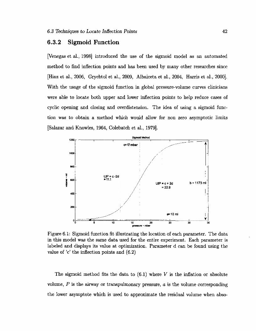
6.1 Sigmoid function fit illustrating the location of each parameter. The
data in this model was the same data used for the entire experiment.
Each parameter is labeled and displays its value at optimization. Pa
rameter d can be found using the value of 'c' the inflection points and
(6.2) 42
6.2 Two examples of a sigmoid and linear spline fitted pressure-impedance
curves with inflection points. The pressure-impedance data was se
lected from the indicated spot in the EIT lung image in the top left
corner. It can be seen from the sigmoid graphs that most often both IP
are not found, while the linear spline method is always able to locate
an IP 46

LIST OF FIGURES xii
7.1 Example outputs from each stage of the algorithm. Starting with in
flection point location the algorithm works toward fuzzification using
the IP found the previous stage for the membership graphs. Once ap
plying the rule base the premise is created and shown clearly. Finally
each pixel is average and the PEEP is selected as shown in the last
column 49
7.2 Trapezoidal Fuzzy Membership graph. This is the type of membership
graph used within the designed algorithm 53
8.1 How frequent each curve fitting method was able to locate an IP. The
box around the median line represents the 75th to 25th quartile. The
dashed lines outside of the box indicates the max and min values. . . 58
8.2 Difference in IP between the Sigmoid and Linear methods. The boxes
around the median line represent the 75th to 25th quartile while the
dashed line represents the max and min for each difference. A lack of
comparative data is indicated in Patients with no quartile boxes. N/A
signifies patients in which neither algorithm was able to locate an IP
in the same pixel 60
8.3 Histogram of the minimum and maximum pressures for all patients.
The maximum pressure for the inflation and deflation limb are the same. 61
8.4 Examples of both 'good' and 'bad' case scenarios encountered during
the visual heuristic experiment. The PI data is taken from the pixel
shown in the EIT image in the top left corner 64
LIST OF FIGURES xiii
8.5 Box plot showing the difference in IP from the human heuristics
method and the linear spline method. The boxes around the median
line represents the 75th to 25th quartile while the dashed lines represents
the max and min for each difference 65
8.6 Box plot showing the difference in IP from the human heuristics
method and the linear spline method. The boxes around the median
line represents the 75th to 25th quartile while the dashed lines repre
sents the max and min for each difference. A lack of comparative data
is represented by no quartile box surrounding the median. N/A means
the sigmoid method was unable to find an inflection points for any of
the four pixels 66
8.7 The progressive change of lungs regions as the pressure increases and
decreases. The classifications are derived from the fuzzy logic system
and show the progressive change from collapse to overdistended as the
pressure increases. This figure also demonstrates the heterogeneous
nature of the lungs 69
8.8 Difference and average of the optimal PEEP found between FSP and
FSe 70
8.9 Difference and average of the optimal PEEP for both FLS and
[Takeuchi et al., 2002] suggested PEEP of using LIP-t-2 mbar. Within
Fig. 8.9b the circles indicate further analysis was performed 73
8.10 Difference between the human heuristic method and the linear spline
m e t h o d f o r t h e l o w e r i n f l e c t i o n p o i n t o n t h e i n f l a t i o n l i m b o n l y . . . . 7 4
8.11 Global PI curve with LIP, UIP, and the LIP+2 mbar pressure and the
Fuzzy optimal selection with according FLS based pressure 75

LIST OF FIGURES xiv
8.12 The PEEP suggested using both Pressure based and EIT based sys
tems. Each data point represents a patient. Prom the figure it can be
seen the inflation limb suggested PEEP is lower compared to respective
deflation suggested PEEP 76
9.1 Algorithm improvement Tree Chart 78
B.l Locations of the pixels used in the visual heuristic experiment 90

List of Tables
4.1 Initial inverse model settings used for pre-analysis stage of the data. . 24
5.1 Fuzzy Operators 30
7.1 Details on creating the trapezoidal based fuzzy membership functions 52
7.2 Rule base table for the first and second fuzzy systems 54
8.1 Mean, standard deviation, and median difference between the sigmoid
and linear inflection points averaged over all patients. The units are in
mbar. For a graphical representation refer to Fig. 8.2 59
8.2 Correlations used to explain large Inflection Point difference between
the Sigmoid and Linear method 62
8.3 [Wu and Mendel, 2011] criteria for testing IF-THEN systems 67
8.4 Results of the difference comparison for the optimal PEEP between
Fuzzy Rule System p and e 70
8.5 Results of the comparison between Fuzzy Rule system p and e with
[ T a k e u c h i e t a l . , 2 0 0 2 ] r e s u l t o f L I P + 2 m b a r a s a g o o d P E E P . . . . 7 1
xv

LIST OF TABLES
B.l Results from the comparison between the visual heuristics and the
three piece linear methods. The table is formatted such that the first
values indicate the median difference followed by it's standard devi
ation for the lower inflection points and then the median difference
followed by it's standard deviation for the upper inflection point all for
pixel 1. Prom here the pattern repeats for the last three pixels

List of Acronyms & Terminology
ALI Acute Lung Injury
ARDS Acute Respiratory Distress Syndrome
CT Computed Tomography
EIDORS Electrical Impedance and Diffuse Optics Reconstruction Software
EIT Electrical Impedance Tomography
FEM Finite Element Method
FLS Fuzzy Logic System
GREIT Graz consensus Reconstruction algorithm for EIT
IP Inflection Points
LIP Lower Inflection Point
PAOP Pulmonary Artery Occlusion Pressure
PEEP Positive End-Expiration Pressure
PI Pressure-Impedance
PV Pressure-Volume
UIP Upper Inflection Point
VILI Ventilator Induced Lung Injury
xvii

Part I
Background
1

Chapter 1
Introduction
Ventilator Induced Lung Injury (VILI) is a serious condition associated with sub-
optimal settings within mechanical ventilation of Acute Lung Injury (ALI) patients.
Its main causes are: 1) cyclical opening and closing of collapsed lung tissue occurring
at low pressures and 2) overdistension of lung tissue occurring at high pressure. The
purpose of this thesis was to investigate the use of Electrical Impedance Tomography
(EIT) as a technology to help reduce VILI. Automated algorithms to process EIT
data and make clinical assessments were developed and retrospectively tested.
EIT is an impedance based, non-invasive, and non-ionizing modality. It estimates
the impedance distribution within a medium using electrical stimulation and volt
age recordings at surface electrodes. This technique is relatively inexpensive and is
an easy-to-use medical device for continuous bedside usage. It has medical applica
tions in the fields of monitoring of pulmonary and cardiac functions, measurement of
brain function, detection of hemorrhages, measurement of gastric imaging, detection
and classification of tumors in breast tissue, and functional imaging of the thorax
[Holder, 2004]. This thesis focused on the functional imaging of the thorax.
Using EIT, clinicians are now able to record the functional behavior of the lungs

1.1 Thesis Objective 3
during a mechanical ventilation recruitment maneuver. EIT thus provides information
for regional behavior and regional pressure-volume relations. It has been shown that
air distribution within the lungs is heterogeneous [Grychtol et al., 2009, Harris, 2005,
Andersen, 2008, Hasan, 2010] giving rise to erroneous recordings when considering
global measurements. This thesis examines the use of EIT to categorize regions as
collapsed, normal or overdistended which can then be used to suggest pressure settings
to reduce VILI [Borges et al., 2006, Venegas et al., 1998, Takeuchi et al., 2002].
1.1 Thesis Objective
This thesis proposes a new method for the selection of mechanical ventilation settings
from EIT data. The objective was split into two separate sections. The first was to
use the EIT data along with pressure data, taken from the ventilation protocol, to
locate regional inflection points from the pressure-impedance graphs. Such graph
and inflection points can be seen in Fig. 6.2. The second was to create an automated
system to use the fitted data to classify the lung regions as normal, overdistended, or
collapsed. The algorithm is described in Chapter 7.
1.2 Thesis Contributions
This thesis looks into the use of a new technique for the location of regional inflection
points (IP) from a short-time based low-flow recruitment maneuver. The regional
inflection points are then used in a novel way within a Fuzzy Logic System (FLS) to
produce a suggested pressure. The thesis contributions are divided into three separate
sections and are listed below.
T-l Summarize scholarly papers on acute respiratory distress syndrome (ARDS) -

1.2 Thesis Contributions 4
Reading and summarization of numerous papers on the topics ARDS, acute
lung injury (ALI) and mechanical ventilation for a single source of knowledge
on this topic.
T-2 EIT based methodology feature extraction - Using EIT and its associated re
gional data on the air movement in lungs, inflection points are located using a
piece wise linear regression technique.
T-3 Using the IP obtained earlier a Fuzzy Logic System (FLS) was designed to
classify the regions as being in healthy or injured. The location of the suggested
pressure was found by maximizing the healthy states while minimizing injured
states.

Chapter 2
Lung Injury
This chapter is broken into three descriptive sections. The first being a description
of Acute Lung Injury (ALI), the second of Ventilator Induced Lung Injury (VILI),
and the third a description of Pressure-Volume (PV) curves. This overview of lung
disease and clinical assessment tools motivates the technical work of further chapters
in this thesis.
The lung is an essential organ within the respiratory system with its main function
being the transport of oxygen into the bloodstream and moving carbon dioxide out
of the bloodstream. Respiratory failure is a medical condition where the patient is
unable to adequately control blood-gases transactions. It can come on abruptly as
seen with acute respiratory failure or slowly as seen with chronic respiratory failure.
Typically, respiratory failure initially affects the transfer of oxygen to the blood or the
removal of carbon dioxide from the blood [Schraufnagel, 2010]. Oxygenation Failure
usually is a sign of ALI and is discussed in this thesis. For further information
on Ventilatory Failure (failure to remove carbon dioxide) refer to Chapter 20 from
[Schraufnagel, 2010].

2.1 Acute Lung Injury 6
2.1 Acute Lung Injury
Acute Lung Injury is the umbrella term used to describe hypoxemic respiratory fail
ure. ALI covers Acute Respiratory Distress Syndrome but also other milder degrees
of lung injury [Schraufnagel, 2010]. ARDS is respiratory failure that results from
widespread injury to the lungs and is characterized by fluid in the alveoli (pulmonary
edema) with an abnormally high amount of protein in the edematous fluid and by
hypoxemia [Merriam-Webster, 2010]. Two types of ARDS exist, the first is primary
which is caused by direct injury and include inhalation based injury, near-drowning,
and pneumonia. Secondary ARDS is caused by a chain of causation including burns
and multiple blood transfusions [Hasan, 2010, Neligan, 2006].
The definition of ALI was clarified and categorized into four observations.
[Hasan, 2010, Bernard et al., 1994].
1. Acute onset of respiratory failure (Minutes to Hours after injury)
2. Diffuse, bilateral pulmonary infiltrates on radiological images
3. Severe hypoxemia
4. Absence of a raised pulmonary artery occlusion pressure (PAOP)
Severe hypoxemia is quantified as the ratio of PAOP over inspired oxygen con
centration ()• Peer defined thresholds for ALI and ARDS have been defined as
266 < < 400 mbar for ALI and < 266 mbar for ARDS. These thresh
olds help determine if a patient has undertaken severe hypoxemia or not. If the
PAOP is > 24 mbar it is considered raised thus anything less would satisfy criteria 4
[Hasan, 2010],
Normal alveoli have an inner layer of surfactant which helps to keep the lung tissue
open during expiration, in diseased lungs this surfactant is lacking making the alveoli
2.2 Ventilated Induced Lung Injury 7
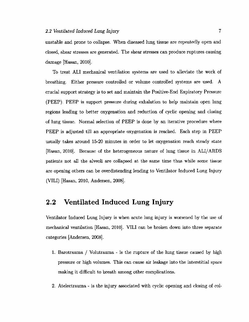
unstable and prone to collapse. When diseased lung tissue are repeatedly open and
closed, shear stresses are generated. The shear stresses can produce ruptures causing
damage [Hasan, 2010].
To treat ALI mechanical ventilation systems are used to alleviate the work of
breathing. Either pressure controlled or volume controlled systems are used. A
crucial support strategy is to set and maintain the Positive-End Expiratory Pressure
(PEEP). PEEP is support pressure during exhalation to help maintain open lung
regions leading to better oxygenation and reduction of cyclic opening and closing
of lung tissue. Normal selection of PEEP is done by an iterative procedure where
PEEP is adjusted till an appropriate oxygenation is reached. Each step in PEEP
usually takes around 15-20 minutes in order to let oxygenation reach steady state
[Hasan, 2010]. Because of the heterogeneous nature of lung tissue in ALI/ARDS
patients not all the alveoli are collapsed at the same time thus while some tissue
are opening others can be overdistending lending to Ventilator Induced Lung Injury
(VILI) [Hasan, 2010, Andersen, 2008].
2.2 Ventilated Induced Lung Injury
Ventilator Induced Lung Injury is when acute lung injury is worsened by the use of
mechanical ventilation [Hasan, 2010]. VILI can be broken down into three separate
categories [Andersen, 2008].
1. Barotrauma / Volutrauma - is the rupture of the lung tissue caused by high
pressure or high volumes. This can cause air leakage into the interstitial space
making it difficult to breath among other complications.
2. Atelectrauma - is the injury associated with cyclic opening and closing of col
2.3 Pressure - Volume Curves 8
lapsed alveoli and is commonly caused by lack of pressure or volume to maintain
open alveoli.
3. Biotrauma - is the increase in pulmonary and systemic inflammatory mediators.
This tends to be a major source of death in ARDS patients as the inflammatory
mediators can lead to organ failure This tends to occur during cyclic opening
and closing of lung units.
Injuries in ventilated ARDS patients can lead to further alveolar ruptures causing
complications such as pneumothorax. This case tends to happen when excess airway
pressures is used. Commonly referred to barotrauma or alveolar overdistension. In
addition to overdistension injury from ventilation systems can be caused by cyclic
opening and closing of lung units. This cyclic action releases cytokines, a protein
transmitter released during inflammatory response. This can be remedied by keeping
lung units open via PEEP thus reducing the opening and closing behavior but insur
ances must be made on the max pressure or volume to avoid overdistension which
can lead to barotrauma [Neligan, 2006]. Another notable factor in ventilation related
injury is the level of inspiration fraction of 02 (Fi02). High F/02 can cause lung
regions to be vulnerable to collapse as the high level of oxygen gets rapidly absorbed
into the blood stream [Neligan, 2006].
2.3 Pressure - Volume Curves
Pressure-volume curves were used in 1946 to measure the mechanical function of the
respiratory system. They were first used to diagnose ALI/ARDS patients in 1976,
since ALI patients would have different mechanical properties compared to healthy
lung patients. The curves were used to diagnose the progress of ALI patients in 1984,
2.3 Pressure - Volume Curves 9
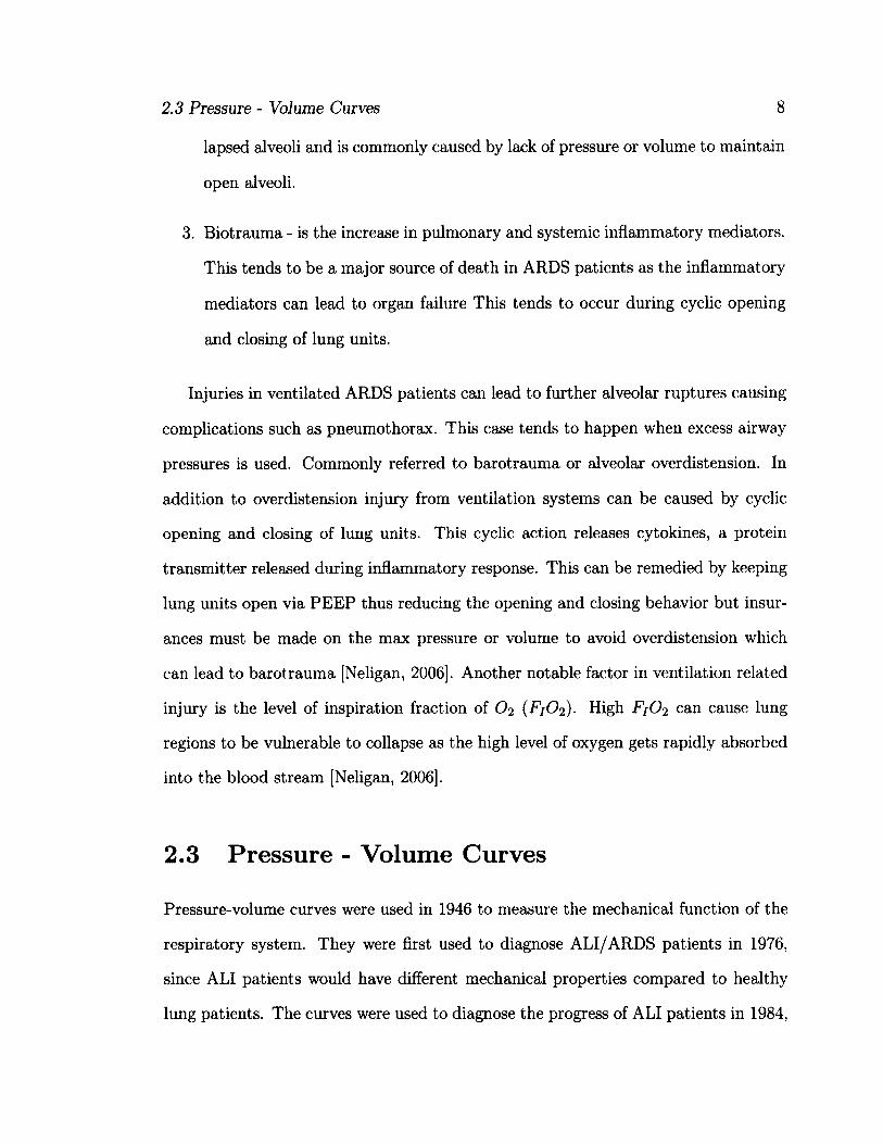
and in 1998 it was used as a means to guide ventilation settings [Andersen, 2008].
An example of a pressure-volume (PV) curve with its associated pressure-impedance
(PI) curve is shown in Fig. 2.1. From the PV/PI curves IP can be located for the use
in guided ventilation strategies.
2000 ^̂
-5001 i i - i_. , . j 0 5 10 15 20 25
Pressure [mbar]
£ UJ
Figure 2.1: An example of a pressure-volume and pressure-impedance curve for both inflation and deflation limbs. From these curves inflection points can be found to be used within guided ventilation strategies. For more information on inflection points refer to Chapter 6
2.3.1 Models of Respiratory Function
There exist two main types of PV curves, static and dynamic. Both measure pressure
and volume from the mouth but are performed differently and thus measure different
physiological functions. (2.1) represents the relationship between airway pressure and
volume where Pao is pressure at the airway opening, V is the lung volume, C is the
respiratory system compliance, V is the gas flow, R is the airway resistance, V is the
convective gas acceleration, I is the impedance, and Pmus is the pressure generated
from respiratory muscles [Harris, 2005].
2.3 Pressure - Volume Curves 10
PAO = ̂ + VR + VI-Pmus (2.1)
Dynamic PV loops are obtained during a gas-flow intensive maneuver. From
(2.1) we can see that dynamic PV curves will cause the resistive and impedance
components to play a factor in the airway pressure. The respiratory muscles play a
role in the airway pressure; thus, if the patient is inadequately sedated the recorded
PV curve may be illustrating factors other then compliance. For the purpose of lung
mechanics the compliance is of most importance as it represents ease of which lung
tissue is ventilated so removal of the resistive, impedance, and respiratory muscles
components are ideal. To remove the unwanted components from (2.1) static PV
curves are used. Static PV curves use very slow airflow (near 0) causing the resistive
component to be minimized. To reduce the impedance factors a constant airflow needs
to be used causing the derivative to be zero. Removing the unnecessary components
is beneficial as the resulting measurements will closely model the static compliance
rather then the dynamic [Andersen, 2008, Hasan, 2010]. There exist three methods
to acquire static PV curves.
1. Super syringe method is done by applying a syringe to the intubation tube and
apply air in steps of 50 to 100ml till a max of 1.51 or 3.01 or 40 to 45 mbar of air
have been applied. Between each step the air flow is ceased for 3 to 10 seconds
to ensure static conditions are reached. The maneuver is slow and forces the
patient to be disconnected from the ventilation system itself but also removes
the resistive and impedance components of the respiration systems thus leaving
the elastic components. The inflation maneuver alone takes between 45-60sec.
[Andersen, 2008, Hasan, 2010, Lu et al., 1999].
2. Constant flow technique is a quasi-static method which does not require removal
2.3 Pressure - Volume Curves 11
of the patient from the ventilation system. It performs a single inflation and
deflation maneuver with constant flow all while taking continuous measurements
of the pressure and volume. The slow flow is done to minimize the resistive
component, with the constant property removing the impedance factor. Studies
have shown that a flow < 9L / min will suffice with larger flows producing
right shifts in the PV curves when compared to static versions [Andersen, 2008,
Harris, 2005, Hasan, 2010, Lu et al., 1999].
3. Multiple occlusion technique consists of various plateau volumes. At each
plateau occlusion measurements are taken, once during inspiration and the
second during expiration. Each measurement only takes 3 seconds and any
volume decrease due to oxygen intake is considered negligible. Similar to the
constant flow technique the patient does not need to be removed from the ven
tilation system but does require sedation to ensure no spontaneous breaths are
taken during the procedure. The procedure lasts between 5 and 10 minutes
[Andersen, 2008, Hasan, 2010, Lu et al., 1999].
For this thesis the [Pulletz et al., 2011] data was used which consisted of a slow
constant flow maneuver with rates of 4 1/min. Each patient was also sedated to
remove the thorax muscle response. More details on the data and patients involved
are listed in Chapter 4.

Chapter 3
Electrical Impedance Tomography
EIT is an imaging modality that is non-invasive, non-ionizing and relatively inex
pensive (thousands of dollars) [Boyle, 2010]. It produces a 2D conductivity image
of a medium. With respect to imaging lung aeration the volumetric accuracy of an
EIT system is within 10% of spirometric measurements [Holder, 2004]. EIT applies
low frequency current (50kHz and max 5mA) and measures the difference voltage
through electrodes on the surface of the medium [Boyle, 2010, Holder, 2004]. The
imaging system uses Finite Element Models to solve the forward problem where
it simulates the voltage on the medium surface with known current and conduc
tivity distribution of the medium. The reconstruction of EIT will be further dis
cussed in Chapter 4. In Canada, EIT machines used with human patients must first
comply with the International Electrotechnical Commission standard 60601-1 and
must be reviewed by a certified laboratory like the Canadian Standards Association
[Boyle, 2010]. The introduction of the EIT system for human studies occurred in
the mid 1980s, with the first written book in 1990 [Holder, 2004]. Starting in the
field of mineral exploration it moved to the biomedical domain in the early 1980s
[Holder, 2004, Allud and Martin, 1977]. Measuring the conductivity of a medium
3.1 EIT in Mechanical Ventilation 13
EIT allows for a new look at the distribution of air, blood, and extravascular liq
uid within the lungs [Adler et al., 1997]. Having gone through rigorous validation,
[Hinz et al., 2003b, Victorino et al., 2004, Gattinoni et al, 1987] EIT is now taking
the next step into specific applications with focus on lung-air distributions.
3.1 EIT in Mechanical Ventilation
Using EIT to measure lung aeration provides increased measurement accuracy and
allows for better PEEP selection for ventilation systems. This is of particular signif
icance given that thoracic CT scans reveal heterogeneity of air distribution within a
pathological lung [Gattinoni et al., 1987]. CT images are considered a gold stan
dard for detailed images of the thorax but they require moving an unstable pa
tients to the imaging area and expose the patient to ionizing radiation making it
a poor choice for repeated bedside use. EIT on the other hand is non-ionizing
and is capable of measuring the distribution of air within the thorax. For in
stance with a current input of 50kHz the resistivity of deflated lung tissue is 12.5
Q • m while inflated lung tissue has a resistivity of around 25.0 fi • m [Holder, 2004].
With this large difference in resistivity between inflated and deflated lung tissue
EIT has been recommended for regional lung monitoring [Hahn et al., 1996]. In
the past global PV curves were used to locate IP and were used to set PEEP ac
cordingly [Hinz et al., 2006, Papadakis and Lachmann, 2007]. It has come to knowl
edge that within ALI patients the distribution of air within the lungs is hetero
geneous making global PV measurements too general to customize PEEP choices
[Victorino et al., 2004]. EIT provides regional conductivity information and is able
to produce pressure-impedance curves where pressure settings can be extracted. With
all the advancements in this field much work still needs to be done by standardizing
3.1 EIT in Mechanical Ventilation 14
inflection point detection algorithms and features to use for classification systems.
The use of EIT in mechanical ventilation is still in a inchoate stages of develop
ment. Early studies using EIT in the lung domain focused primarily on validation
[Hahn et al., 1996, Frerichs et al., 2002, Hinz et al., 2003a, Victorino et al., 2004].
Subsequent research worked toward extracting information, like inflection points and
pressure-impedance curves, and drawing conclusions related to the state of lung tis
sue [Kunst et al., 2000, Gattinoni et al., 1987, Amato et al., 1998, Kunst et al., 1999,
Genderingen et al., 2004, Adler et al, 2012], More research is necessary to un
derstand guided ventilation strategies, create automated systems, to determine
accurate rule bases and incorporate uncertainty into the Fuzzy Logic Systems
[Grychtol et al., 2010, Luepschen et al., 2007].
Research comparing global and regional PV curves shows that the former can be
represented as a sum of the latter [Kunst et al., 2000]. Using PV curves to identify
therapeutic pressure to reduce VILI has been confirmed. Chapter 6 further elaborates
on the use of PV curves and inflection points. Furthermore, [Kunst et al., 2000,
Kunst et al., 1999] noticed that dependent regions have higher LIP then the counter
parts in the non-dependent region. The airs dependency on gravity increases collapsed
regions in the direction of gravity. This gravitational dependency helps explain the
continual recruitment along the linear portion of a global PV curve and the need for
a regional bedside imaging systems like EIT.
The regional information provided by EIT clarifies the understanding of ven
tilation distributions, locating regions of overdistension and regions of collapse,
one sided ventilation, regional compliance, LIP and UIP, and delays in ventilation
[Adler et al., 2012]. The reconstruction system used for this thesis produced images
of size 32x32 pixels. The average lung-region of interest (lung-ROI) for all patients
was 248.88 ± 53.33 pixels. From Chapter 4 the average height for all patients was
3.1 EIT in Mechanical Ventilation 15
177 ± 9 cm. Using the median relationship between external chest size and height
from [Todd, 2010], which can be seen in (3.1), a max circumference of 105.4 cm
and minimum circumference of 95.2 cm was found. This resulted in a resolution of
3.38 ± 0.923 cm2 per pixel. The resolution value is an approximation due to the use
of lung-region of interest and the relationship matching external chest size to height.
Using the chest-region of interest of which the size is 575 pixels for all patients as a
replacement for the lung-ROI a resolution of 1.39 cm2 per pixel is realized. It can
then be argued that the resolution for this particular EIT system is between 1.39 and
3.38 ± 0.923 cm2 per pixel.
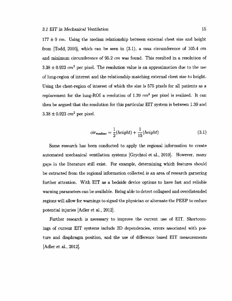
cirmedian = ^ (height) + ̂ (height) (3.1)
Some research has been conducted to apply the regional information to create
automated mechanical ventilation systems [Grychtol et al., 2010]. However, many
gaps in the literature still exist. For example, determining which features should
be extracted from the regional information collected is an area of research garnering
further attention. With EIT as a bedside device options to have fast and reliable
warning parameters can be available. Being able to detect collapsed and overdistended
regions will allow for warnings to signal the physician or alternate the PEEP to reduce
potential injuries [Adler et al., 2012].
Further research is necessary to improve the current use of EIT. Shortcom
ings of current EIT systems include 2D dependencies, errors associated with pos
ture and diaphragm position, and the use of difference based EIT measurements
[Adler et al., 2012].

Chapter 4
Data and EIT Reconstruction
This chapter describes the data and reconstruction algorithm used within this thesis.
The first section covers the number of patients dividing them into ALI and control.
It also covers the ventilation protocol along with the mechanical ventilation unit and
the EIT system used in the measurements. Data pre-analysis is explained in the data
section of this chapter and covers EIT-pressure-alignment and locating the start and
end of the pressure ramp aka the recruitment maneuver.
In the second section the algorithm used to reconstruct the EIT data is described
with focus on the parameters used, a description of the reconstruction, and the ad
vanced nature of the algorithm.
4.1 Data
The data was obtained from [Pulletz et al., 2011] where a low-flow pressure based
recruitment maneuver with synchronized EIT was performed.
4.1 Data
4.1.1 Patients
17
The data used for this thesis was of human trials from the medical university center
at Schleswig Holstein campus in Kiel. The experiment received local ethics approval
for 26 patients. The patients were taken from the surgical intensive care unit and
the operations theaters with written consent provided from each patient or a legal
representative. All of the patients within the study were sedated, paralyzed and
artificially ventilated using a pressure controlled ventilation mode while in the supine
position. The distribution of the patients consisted of 8 healthy lung patients (age:
41 ± 14 years, height: 177 ± 8cm, weight: 76 ± 8 kg, mean ± SD) and 18 ALI
patients, (age: 58 ± 14 years, height: 177 ± 9 cm, weight: 80 ± 11 kg) which fulfilled
the American-European consensus criteria for ALI (rapid onset, < 300 mmHg,
bilateral infiltrates, and no clinical sign for left atrial hypertension.
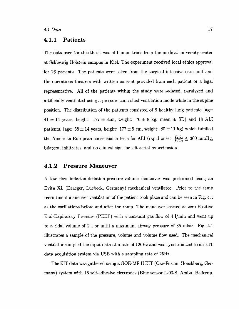
4.1.2 Pressure Maneuver
A low flow inflation-deflation-pressure-volume maneuver was performed using an
Evita XL (Draeger, Luebeck, Germany) mechanical ventilator. Prior to the ramp
recruitment maneuver ventilation of the patient took place and can be seen in Fig. 4.1
as the oscillations before and after the ramp. The maneuver started at zero Positive
End-Expiratory Pressure (PEEP) with a constant gas flow of 4 1/min and went up
to a tidal volume of 2 1 or until a maximum airway pressure of 35 mbar. Fig. 4.1
illustrates a sample of the pressure, volume and volume flow used. The mechanical
ventilator sampled the input data at a rate of 126Hz and was synchronized to an EIT
data acquisition system via USB with a sampling rate of 25Hz.
The EIT data was gathered using a GOE-MFII EIT (CareFusion, Hoechberg, Ger
many) system with 16 self-adhesive electrodes (Blue sensor L-00-S, Ambu, Ballerup,
4.2 EIT Reconstruction 18
•e 20 (0 115
1 10 £ 5
Q. 0
20 40 60 80 100 120 140 160 180 200
„ 1500 E I 1000
I 500
0 20 40 60 80 100 120 140 160 180 200
40
| 20
| °
u. -20
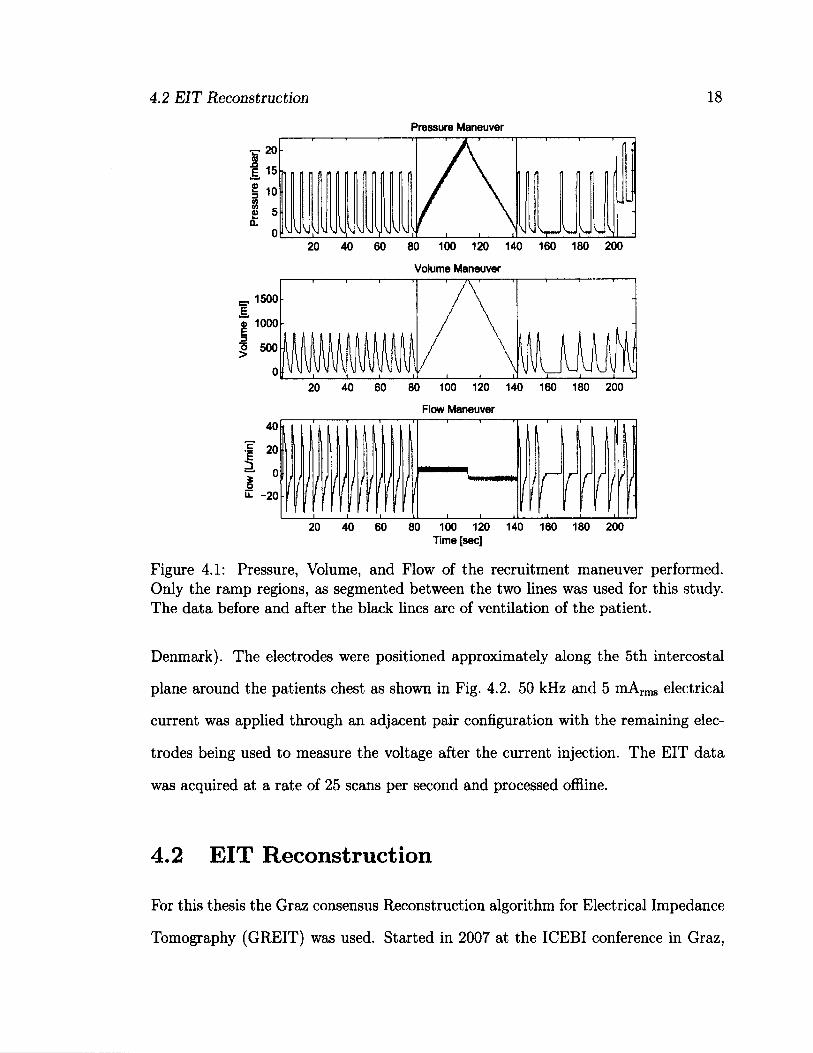
Figure 4.1: Pressure, Volume, and Flow of the recruitment maneuver performed. Only the ramp regions, as segmented between the two lines was used for this study. The data before and after the black lines are of ventilation of the patient.
Denmark). The electrodes were positioned approximately along the 5th intercostal
plane around the patients chest as shown in Fig. 4.2. 50 kHz and 5 mArms electrical
current was applied through an adjacent pair configuration with the remaining elec
trodes being used to measure the voltage after the current injection. The EIT data
was acquired at a rate of 25 scans per second and processed offline.
Pressure Maneuver
%
-1 —r T
A / \ - •J
\ \ \ V V \ \ \ \ V V \ \ 1 ( \ i i i V-L, L L \
volume Maneuver
Flow Maneuver
20 40 60 80 100 120 140 160 180 200 Time [sec]
4.2 EIT Reconstruction
For this thesis the Graz consensus Reconstruction algorithm for Electrical Impedance
Tomography (GREIT) was used. Started in 2007 at the ICEBI conference in Graz,
4.2 EIT Reconstruction 19
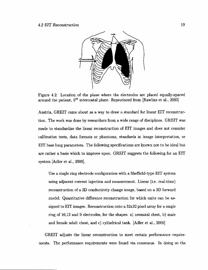
Lungs
Figure 4.2: Location of the plane where the electrodes are placed equally-spaced around the patient, 5th intercostal plane. Reproduced from [Rawlins et al., 2003]
Austria, GREIT came about as a way to draw a standard for linear EIT reconstruc
tion. The work was done by researchers from a wide range of disciplines. GREIT was
made to standardize the linear reconstruction of EIT images and does not consider
calibration tests, data formats or phantoms, standards in image interpretation, or
EIT base lung parameters. The following specifications are known not to be ideal but
are rather a basis which to improve upon. GREIT suggests the following for an EIT
system [Adler et al., 2009].
Use a single ring electrode configuration with a Sheffield-type EIT system
using adjacent current injection and measurement. Linear (i.e. real-time)
reconstruction of a 2D conductivity change image, based on a 3D forward
model. Quantitative difference reconstruction for which units can be as
signed to EIT images. Reconstruction onto a 32x32 pixel array for a single
ring of 16,12 and 9 electrodes, for the shapes: a) neonatal chest, b) male
and female adult chest, and c) cylindrical tank. [Adler et al., 2009]
GREIT adjusts the linear reconstruction to meet certain performance require
ments. The performance requirements were found via consensus. In doing so the
4.2 EIT Reconstruction 20
reconstruction algorithm modifies its minimization criteria thus not satisfying the
underlying mathematical model. A linear reconstruction algorithm is used rather
then an iterative approach as they tend to fail. The failure is brought upon by mea
surement noise and geometric uncertainty in clinical and experimental EIT data. A
linear approach also facilitates real-time reconstruction.
The GREIT inverse model R differs depending on the choice of the forward model,
noise model, and the desired performance metrics. The forward model allows calcula
tions of voltage differences, y^, from a conductivity change, x^k\ where k represents
the indices for the training set. The forward model provides the details of the body's
geometry, the electrode size and contact impedance, and the reference conductivity
(<7r) around which conductivity changes occur. GREIT uses a 3D FEM forward model
using the complete electrode model [Adler et al., 2009]. From the forward model the
measurement variance is calculated.
For the noise model the measurement data from the forward model is used.
In GREIT two sources of noise are considered: electronic measurement noise, and
electrode movement artifacts. The electronic measurement noise can be modeled
as various distributions but uniform Gaussian is acceptable for generic EIT recon
struction and was used. The measurement noise is usually related to the EIT
hardware and patient connections such as different gain settings on each chan
nel. Electrode movement artifacts happen when electrodes move with posture or
chest movement during breathing and have reported to cause significant artifacts
[Adler et al., 1996, Zhang and Patterson, 2005, Coulombe et al., 2005]. To reduce
the noise, augmented forward models based on both the conductivity change and
electrode movement can be made to reduce the artifacts. This is currently imple
mented by deformations of the FEM but can be based on a calibration protocol in
an implemented system.

4.2 EIT Reconstruction 21
Using the desired performance metrics, training is performed to find a well suited
reconstruction matrix. This is done by using "desired images" , x[k\ in a training
set of size (k) . The "desired images" correspond to locations of conductivity in the
forward model, x[k). xt is centered at the same location as xt but is designed to
be circular and have an accompanying blur radius around the center. The use of
the desired image allows for uniform resolution throughout the entire image at the
expense of lower resolution along the boundaries. For each "desired image" a weight
image is created to put weights to each pixel within the "desired image". These
weights are used to put more emphasis on some metrics rather than others. For
each "desired image" there exist two circular regions, the first is centered around the
targeted position to emphasis a flat amplitude while the second regions is outside of
the first and represents a region in which the amplitude is to be zero. In between
the two regions the desired image is supposed to smoothly transition from the inner
region amplitude to zero, the outer region. Larger weight is given to these regions to
enforce that performance metrics are met while smaller weights are selected for the in
transition region to allow the algorithm to have flexibility to meet other specifications.
In addition to the conductivity targets, noise training samples are used for elec
tronic noise and movement artifacts. For noise training the desired image (x^)is
zero. The weight image (w^) is large to enforce a penalty on noise.
Based on the forward model, noise model, and desired performance an improved
GREIT reconstruction matrix can be created by solving the minimization express for
error e2 as seen in (4.1).
4.2 EIT Reconstruction 22
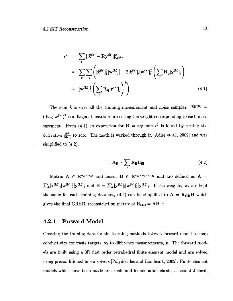
e2 = X>(k)-Ry(k,llw<'.> k
= E E ([*(k,i;Vk,tf - 2[x<k>],[w"'>]? ̂ Rub-c'ij j
+ [w (k ,]?feRiity<k)]>)) <41)
The sum k is over all the training measurement and noise samples. W^k) =
(diag w^)2 is a diagonal matrix representing the weight corresponding to each mea
surement. From (4.1) an expression for R = arg min e2 is found by setting the
derivative to zero. The math is worked through in [Adler et al., 2009] and was
simplified to (4.2).
= Au-£R„B l i , (4.2) I
Matrix A € and tensor B G RnArX"MXnM and are defined as A =
Sfc[x(k)]i[w(k)]f[y(k)]j and B = 5^fc[y(k)Mw(k)]?[y(k)]j. If the weights, w, are kept
the same for each training data set, (4.2) can be simplified to A = RgbB which
gives the final GREIT reconstruction matrix of RGB = AB-1.
4.2.1 Forward Model
Creating the training data for the learning methods takes a forward model to map
conductivity contrasts targets, xt to difference measurements, y. The forward mod
els are built using a 3D first order tetrahedral finite element model and are solved
using preconditioned linear solvers [Polydorides and Lionheart, 2002]. Finite element
models which have been made are: male and female adult chests, a neonatal chest,
4.2 EIT Reconstruction 23
(a) Start of Inflation (b) Max Pressure (c) End of Deflation
Figure 4.3: Example reconstructions using the GREIT methods of a healthy lung patient (patient 7). The outer most region in each image is from the reconstruction itself and has no physiological meaning. The second region from the outside in represents the chest and non-lung regions. The third and inner most region represents the lungs. Within the lung region the scale goes from light to dark, with the corresponding impedance going from high to low respectively.
and a cylinder. It is possible to create patient specific FEM which would provide a
better reconstruction but as [Adler et al., 2009] has stated from experience working
with time-difference EIT the four models provided work with most of the accuracy of
an adaptive meshing. For this thesis the male human thorax FEM model was used.
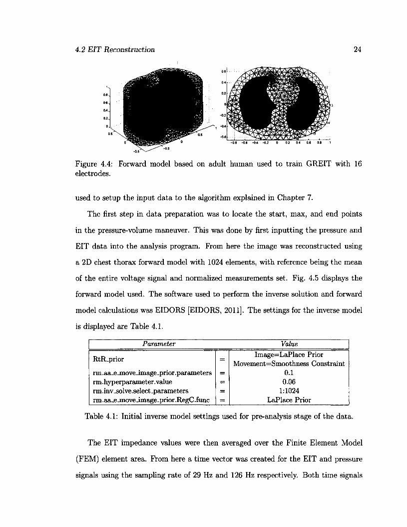
4.2.2 Reconstruction Model Used
For this thesis the adult male model with 16 electrodes was used. The first electrode
was placed on the median dorsal part of the model and the ninth electrode placed
directly across. Fig. 4.4 shows both the 3D model as well as the 2D version with
electrode placement used. The training was done using normalized measurements
with 500 samples of 3% of the model diameter in size targets.
4.2.3 Data pre-analysis
All analysis was done offline with the majority of work being done in the Fuzzy Logic
System FLS. This section explains the code designed by [Pulletz et al., 2011] and was
4.2 EIT Reconstruction 24
Figure 4.4: Forward model based on adult human used to train GREIT with 16 electrodes.
used to setup the input data to the algorithm explained in Chapter 7.
The first step in data preparation was to locate the start, max, and end points
in the pressure-volume maneuver. This was done by first inputting the pressure and
EIT data into the analysis program. From here the image was reconstructed using
a 2D chest thorax forward model with 1024 elements, with reference being the mean
of the entire voltage signal and normalized measurements set. Fig. 4.5 displays the
forward model used. The software used to perform the inverse solution and forward
model calculations was EIDORS [EIDORS, 2011]. The settings for the inverse model
is displayed are Table 4.1.
Parameter Value
RtR_prior = Image=LaPlace Prior Movement=Smoothness Constraint
rm.aa_e_moveJmage-prior.parameters rm.hyperparameter .value rm.inv_solve.select_parameters rm.aa_ejiioveJmage_prior.RegC.func
=
0.1 0.06
1:1024 LaPlace Prior
Table 4.1: Initial inverse model settings used for pre-analysis stage of the data.
The EIT impedance values were then averaged over the Finite Element Model
(FEM) element area. From here a time vector was created for the EIT and pressure
signals using the sampling rate of 29 Hz and 126 Hz respectively. Both time signals
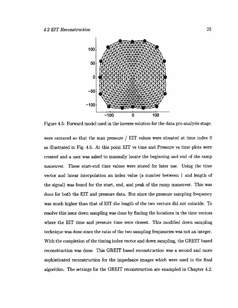
4.2 EIT Reconstruction 25
100
50
0
-50
-100
-100 0 100
Figure 4.5: Forwaxd model used in the inverse solution for the data pre-analysis stage.
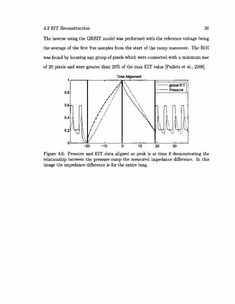
were centered so that the max pressure / EIT values were situated at time index 0
as illustrated in Fig. 4.6. At this point EIT vs time and Pressure vs time plots were
created and a user was asked to manually locate the beginning and end of the ramp
maneuver. These start-end time values were stored for later use. Using the time
vector and linear interpolation an index value (a number between 1 and length of
the signal) was found for the start, end, and peak of the ramp maneuver. This was
done for both the EIT and pressure data. But since the pressure sampling frequency
was much higher than that of EIT the length of the two vectors did not coincide. To
resolve this issue down sampling was done by finding the locations in the time vectors
where the EIT time and pressure time were closest. This modified down sampling
technique was done since the ratio of the two sampling frequencies was not an integer.
With the completion of the timing index vector and down sampling, the GREIT based
reconstruction was done. This GREIT based reconstruction was a second and more
sophisticated reconstruction for the impedance images which were used in the final
algorithm. The settings for the GREIT reconstruction are exampled in Chapter 4.2.
4.2 EIT Reconstruction 26
The inverse using the GREIT model was performed with the reference voltage being
the average of the first five samples from the start of the ramp maneuver. The ROI
was found by locating any group of pixels which were connected with a minimum size
of 20 pixels and were greater than 25% of the max EIT value [Pulletz et al., 2006].
Time Alignment
global EIT Pressure
0.8
0.6 n
0.4
0.2
-20 -10
Figure 4.6: Pressure and EIT data aligned so peak is at time 0 demonstrating the relationship between the pressure ramp the measured impedance difference. In this image the impedance difference is for the entire lung.

Chapter 5
Fuzzy Logic
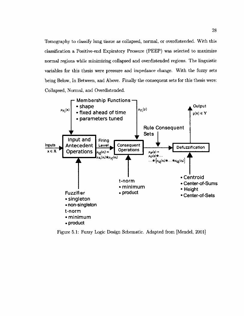
This chapter introduces the theory of Fuzzy Logic Systems (FLS). A FLS is a sequence
of functions and methods which non-lineaxly map data (features) to a scalar output.
It does this by turning crisp values (input data) into fuzzy sets (via fuzzification) and
then back into crisp values (via defuzzification). A FLS is made up of three main
components. 1) The fuzzifier takes the crisp input values(linguistie variables, which
for this thesis are pressure and impedance change) and maps them into fuzzy sets
with a degree of membership valued from 0 to 1. From here the fuzzy sets are passed
to the inference system which is composed of IF-THEN rules. These rules combine
the fuzzy sets by using "AND" or "OR" operators resulting in another set of fuzzy
sets called consequent sets, also with an according membership value. Finally the
consequent sets are passed to the defuzzifier which combines the consequent sets and
calculates a crisp value from the resulting curve. Each block can be seen in Fig. 5.1
with the accompanying decisions which need to be made for each block.
Fuzzy Logic is an excellent way to integrate engineering with expert knowledge.
For this thesis it was a method to mix lung physiology and mechanical ventilation with
medical imaging. In this thesis Fuzzy Logic was used along with Electrical Impedance
28
Tomography to classify lung tissue as collapsed, normal, or overdistended. With this
classification a Positive-end Expiratory Pressure (PEEP) was selected to maximize
normal regions while minimizing collapsed and overdistended regions. The linguistic
variables for this thesis were pressure and impedance change. With the fuzzy sets
being Below, In Between, and Above. Finally the consequent sets for this thesis were:
Collapsed, Normal, and Overdistended.
- Membership Functions — • shape • fixed ahead of time • parameters tuned
Rule Consequent Sets I
Firing Level Inputs
x € X Defuzzification
Consequent Operations
Input and Antecedent Operations
Fuzzifier • singleton • non-singleton t-norm • minimum • product
• • * w • • • W^QJ v*pJJ
t-norm • minimum • product
• Centroid • Center-of-Sums • Height • Center-of-Sets
Figure 5.1: Fuzzy Logic Design Schematic. Adapted from [Mendel, 2001]

5.1 Fuzzifier
5.1 Fuzzifier
29
5.1.1 Fuzzy Sets
Unlike classical sets where the distinction between member and non-member is clear,
{0,1}, fuzzy sets can have a range of membership, [0,1]. The membership value
dictates the degree to which they are associated to the fuzzy set, with higher values
having larger associations. A fuzzy set can have elements which have varying degrees
of membership, unlike classical sets where elements are either associated or not. Since
membership is not complete a single element can have associations with multiple
fuzzy sets. For instance an element (x) with a range of possible values as dictated
by universe X can have memberships to fuzzy sets Fy and F2. The membership for
fuzzy set F\ is indicated as Hfx{x) = 3? where UfAx) € [0,1], similar with F2 but
with different subscripts. The association is performed by a membership function
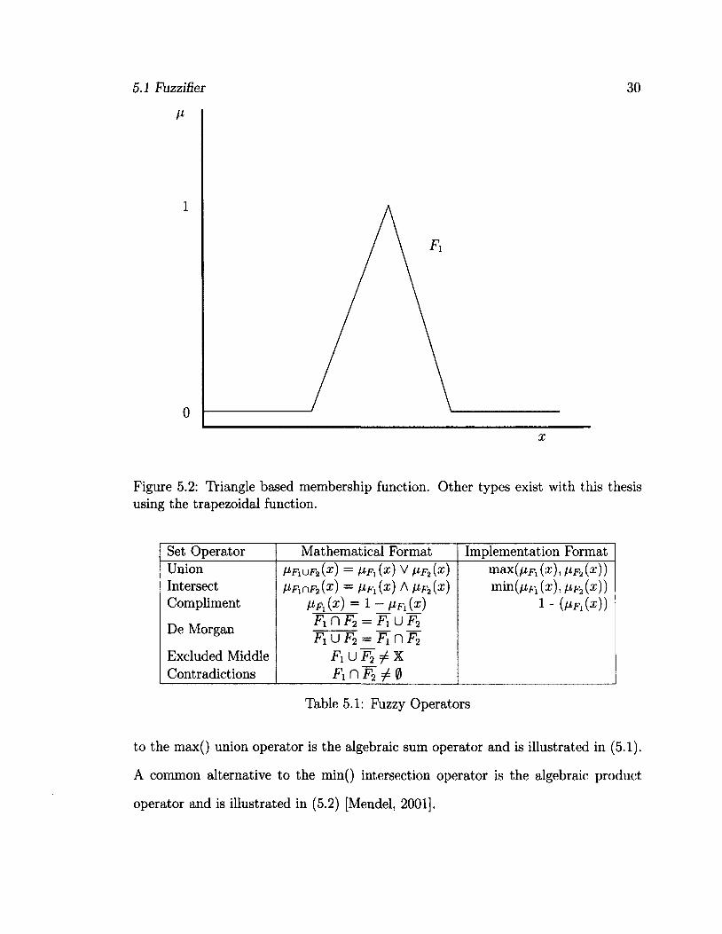
which takes elements, x, and places them in a fuzzy set. Fig. 5.2 displays an example
of a membership function for input variable x and fuzzy set F\. It should be noted
since elements can be associated with multiple fuzzy sets each fuzzy set has its own
membership function.
Fuzzy sets also work with classical logical operations such as those displayed in
Table 5.1. Within Table 5.1 operators which have no implementation can be broken
down into union, intersection, and complement thus are not needed. With respect to
the Law of Excluded Middles and the Law of Contradictions fuzzy logic is incongruent
with classical logic. This is due to the inherent property of fuzzy sets and how they
overlap as do their complements, thus you may never have complete membership or
zero membership depending on which law is applied.
Multiple methods for performing the union and intersection are available and are
referred to as t-conorms (union) and t-norms (intersection). A common alternative
5.1 Fuzzifier 30
1
0
x
Figure 5.2: Triangle based membership function. Other types exist with this thesis using the trapezoidal function.
Set Operator Mathematical Format Implementation Format Union Intersect Compliment
De Morgan
Excluded Middle Contradictions
»F xU F 2{X ) = H F i ( x ) V H F 2 { X ) Mnf2(s) = Hfi{X) A Vf2(X)
H f x { x ) = 1 - f i F l { x ) F\ n F2 = F\ U F2 F\ U F2 — Fi n F2
F1uT2^X FinF 2 5 i0
max ( f j , F l ( x ) , h f 2 {x ) )
m i n ( f j L F l ( x ) , t i F » ( x ) ) 1 " (A*Fi(®))
Table 5.1: Fuzzy Operators
to the max() union operator is the algebraic sum operator and is illustrated in (5.1).
A common alternative to the min() intersection operator is the algebraic product
operator and is illustrated in (5.2) [Mendel, 2001].

5.1 Fuzzifier 31
/^uF 2(X ) = /xFl(x) + HF 2 (X) - ̂F L (X)F IF 2 (X) (5.1)
V F ^ F 2 { x ) = FLF l ( x )FLF2 ( x ) (5.2)
5.1.2 Membership Functions
In a rule based FLS membership functions are used to take crisp values to fuzzy sets
and vice versa. Theses fuzzy sets are then used in the antecedents and conclusions,
refer to Fig. 5.1 to see the input of membership graphs to the two according fuzzy logic
blocks. The main sections of any membership function are the Core, Support, and
Boundary. The core region is the interval where the fuzzy set, for instance Fi, has full
membership i.e. /^(x) = 1. The support region is the interval where membership is
non-zero i.e. Hf-i{x) > 0. The boundary region is the interval where the membership
is between 0 and 1 i.e. 0 < hfx(x) < 1. When designing fuzzy membership functions
it is important to consider carefully the location of these regions as they play a large
role in the performance of a FLS [Sivanandam et al., 2006].
Two types of membership functions exist. One which considers uncertainty in the
data (Type-2) and the other which does not (Type-1). This thesis focuses on Type-
1 systems with extra detail on Type-2 systems available in [Mendel, 2001]. Within
Type-1 systems two different fuzzy membership functions exist, singleton and non-
singleton. The difference between the two is an extra module, which models the datas
uncertainties prior to fuzzification, for a non-singleton systems.
Referring to Fig. 5.1 for a overview of the variable names. For a singleton system
/iX(x) = 1 if x = x' and /zx(x) = 0 for all x ̂ x'. Where x is equal to p crisp elements
each with there own universe, i.e. x = (xi,. . . ,xp)T € Xi x X2 x • • • x Xp = X.
5.2 Inference 32
x' is the crisp input value of interest. Prom here the firing level is calculated by
SUPXieXi^Q'ixi) = where • is a t-norm. For a singleton system
the firing level is simplified since *s non-zero at one location, x, = x\. This
calculated value is now the membership value for the fuzzy set i and for rule I.
Setting up fuzzy membership functions can be done in multiple way, such as;
intuition and neural networks [Mendel, 2001].
5.2 Inference
Fuzzy inferences are IF-THEN based rules from which consequences are derived from.
Connectors between each term in the IF-THEN statement are made up of "AND" or
"OR" which in turn have various mathematical equivalents, t-norms and t-conorms,
respectively. The standard format for most fuzzy rules is IF (linguistic variable 1 is
fuzzy set 1) AND/OR (linguistic variable 2 is fuzzy set 2) AND/OR ... THEN (output
n is consequent n) [Sivanandam et al., 2006]. For instance IF xt is F[ AND/OR
... AND/OR xp is Fp THEN y is Gl. I = I... m and represents the number of
rules, p represents the number of linguistic variables each with their own universe
(xi 6 Xi... xp € Xp) and y € Y output linguistic variable for fuzzy set Gl. It can be
shown that fuzzy systems with multiple outputs can be broken into multiple systems
each with one output [Mendel, 2001].
5.3 Defuzzifier
Defuzzification is the processes of turning fuzzy sets into crisp values. Many methods
of defuzzification exist with a main criteria being computational simplicity. The com
mon ones are: Centroid, Center-of-Sums, Height, and Center-of-Sets [Mendel, 2001].

5.3 Defuzzifier 33
5.3.1 Centroid Method
The centroid method combines the consequent sets by using the max t-norm. B =
u r=xBi.
y (X) = ViUBiVi)
Where i indexes the combined set B . This method is usually difficult to compute
due to the union of the output fuzzy sets, Bl [Mendel, 2001].
5.3.2 Cent er-of- Sums
This method combines the consequent sets by addition. Hb(v) = Then
proceeds to find the centroid of Hb(u)-
r^m ».(X) = B' (5.4)
2_W= 1 aBl
Where cBi is the centroid of the consequent set Bl for rule I and aBi is the area
u n d e r n e a t h t h e c o n s e q u e n t s e t B l f o r r u l e I .
5.3.3 Height Defuzzifier
This method locates the maximum point from the output set via a singleton method.
For multiple maximums the average can be taken. It takes these values and adds
then into a set of size m, and then calculates the centroid of the resulting set.
Where y l is the location of the maximum value with fxBiy l being the according
output set membership value. A common modifier to this method is to scale (5.5) by

5.3 Defuzzifier
some measure of the spread of Hb1{v1)
34
EliM*)/*" (5.6)
5.3.4 Cent er-of- Sets
This method is fairly quick as it replaces the rule consequent set with a singleton
located at the centroid with an amplitude scaled by the firing level, then finds the
centroid of the combined singletons. The firing level (fi) is the combined membership
value for each fuzzy set or T?=1fiFi(xi), where T is short for the t-norm.
y«»(x) = Jl
m (5.7)

Part II
Contributions
35
Chapter 6
Inflection Points
This chapter describes what inflection points (IP) are, how they are found, and their
use with EIT in base pressure suggestion for mechanical ventilation systems. In
this context inflection points are the locations along a pressure-volume/impedance
(PV/PI) curve where the slope dramatically changes usually from a low compliance
region to a high compliance region or a high compliance region to a low one. There
exists multiple ways of locating IP [Harris et al., 2000] with this thesis exploring the
sigmoid method, visual heuristics, and the 3-piece linear spline method. The basis be
hind this thesis is to locate pressure(s) where the alveoli are not in a state of collapse
or overdistension which are known to be large contributors to ventilator induced
lung injury (VILI) [Bigatello et al., 1999, Amato et al., 1998, Borges et al., 2006,
Venegas et al., 1998, Takeuchi et al., 2002]. The use of inflection points in clinical
settings are well known and are currently used to set the base-pressure (PEEP) in
Acute Lung Injury (ALI) patients [Venegas et al., 1998, Harris et al., 2000]. In order
to find inflection points which are meaningful particular ventilation strategies are used
in order to reduce certain physiological effects and are described in detail in Chapter
2.
6.1 What are Inflection Points
6.1 What are Inflection Points
37
Inflection points axe locations on a pressure-volume/impedance curve where alve
oli efficiency increases/decreases dramatically depending on if the pressure is low or
high respectively. There are various ways to locate the lower inflection point (LIP).
The location where the pressure-volume curve starts to have a linear compliance
[Matamis et al., 1984a, Brunet et al., 1995]. The pressure at which rapid increase in
the compliance of the pressure-volume curve occurs [Harris et al., 2000]. Thirdly, to
place two lines one along the low compliance region and the other on the high compli
ance region and locate the intersection [Takeuchi et al., 2002, Gattinoni et al., 1987,
Amato et al., 1995]. Finally find the lower point in which the PV/PI curve first de
viates from its high compliance region [Dambrosio et al., 1997]. All of these methods
provide a distinct indication of a beginning and end of the high compliance regions.
6.2 Importance of Inflection Points
The work on inflection points is important as it is one of the common
methods for optimizing PEEP in mechanical ventilation [Matamis et al., 1984b,
Amato et al., 1998]. Patients in need of mechanical ventilation in particular pa
tients with acute respiratory failure have a high mortality and morbidity rate
[Hudson, 1989]. Mechanical ventilation can damage the lungs [Amato et al., 1998]
causing lesions at the alveolar-capillary interface [Fu et al., 1992], create alter
ations in permeability [Carlton et al., 1990], and cause edema [Tsuno et al., 1990,
Dreyfuss and Saumon, 1993]. VILI is a significant problem when it comes
to critical patients with acute respiratory failure [Slutsky, 1994]. A con
tributing problem to VILI is the cyclic opening and closing of the alveoli
[Ranieri et al., 1999, Pulletz et al., 2011, Mead et al., 1970] and can increase mortal
6.2 Importance of Inflection Points 38
ity. [Amato et al., 1998] showed that two groups (one using protective ventilation
strategies and one without) revealed higher survival rates in the protective ventila
tion group. Prom the experiment 11/29 patients died in the protective ventilation
group while 17/24 died in the non-protective ventilation group. [Amato et al., 1998]
study using human subjects revealed that the length of being on mechanical venti
lation impacted the survival after a 28-day trial period. A great deal of controversy
exists in finding the appropriate PEEP settings with over 9000 papers published in
this topic and no standard conclusion [Rouby et al., 2002]. With the use of EIT in
clinical settings regional information is now available which will help in locating an
optimal PEEP.
Some clinics use the lower and upper inflection points for pressure settings
[Venegas et al., 1998]. In the study conducted by [Brunet et al., 1995] it was shown
that the use of PEEP was able to increase normal regions while being able to decrease
non-aerated regions. A study conducted by [Dambrosio et al., 1997] showed that the
use of PEEP resulted in large reductions of collapsed regions. Albeit the given bene
fits of PEEP, there is a lack of unification amongst researchers on how to locate valid
PEEP readings [Rouby et al., 2002]. Pressure-Volume curves have been suggested for
finding the optimal PEEP value by looking for points which maximize the recruitment
[Gattinoni et al., 1984]. Most current PV curves study the use of global pressure-
volume readings to create a curve which is used to find associated parameters. The
benefits of using global LIP and UIP are visible [Amato et al., 1998, Hinz et al., 2006].
[Hinz et al., 2006, Harris, 2005, Venegas et al., 1998] have suggested the use of UIP
to set as the maximum airway pressure while [Lu et al., 1999, Takeuchi et al., 2001,
Takeuchi et al., 2002, Harris et al., 2000, Venegas et al., 1998] have suggested using
the LIP for the PEEP. It is also suggested that the PEEP should be set from the
deflation limb since the alveoli would be recruited once and tend to collapse at a lower
6.2 Importance of Inflection Points 39
pressure once opened. This idea helps since PEEP is used to maintain open alveoli
not to open them up initially [Papadakis and Lachmann, 2007, Albaiceta et al., 2004,
Takeuchi et al., 2002, Harris et al., 2000].
[Papadakis and Lachmann, 2007] showed that when PEEP was set below
the global LIP damage and collapse occurred most. In the same study by
[Papadakis and Lachmann, 2007] it was also noticed that an increase in recruitment
occurred, up to 40% of the lung, with a pressure set above the lower inflection point.
[Muscedere et al., 1994] showed similar results to [Papadakis and Lachmann, 2007] in
which large amounts of lung tissue were collapsed when PEEP was set to zero and be
low the lower inflection point. Much of the air volume was distributed to the anterior
segments causing overdistension. This phenomenon was likely observed due to the use
of animal subject in supine positions during lavage. When [Muscedere et al., 1994]
set PEEP above the LIP collapse occurred in the early stages and progressively in
flated over 2 hours with large areas expanding first followed by smaller focal areas.
The total airway injury score for the PEEP > LIP group was similar to that of the
control group. A similar independent study was conducted by [Takeuchi et al., 2002]
and found setting the PEEP to LIP-t-2 mbar provided the best compliance and best
arterial oxygen partial pressure at a fraction of inspired oxygen of 0.5. LIP+2 mbar
also minimized lung inflammation and mRNA expression for interleukin - 1/3, which
along with mRNA expression for interleukin-8 are inflammatory responses indicative
of inadequate PEEP [Takeuchi et al., 2002]. [Amato et al., 1995] conducted an ex
periment displaying the benefits of using LIP for PEEP. [Amato et al., 1995] set the
PEEP above the LIP with tidal volume < 6 ml/kg and peak pressure < 40 mbar
and compared it to a volume cycled ventilation with Vt < 12 ml/kg, PEEP set via
FIO2, and normal PaCQ% levels. The experiment found that the first scheme im
proved oxygen-blood transaction in patients with ARDS increasing the chance of
6.3 Techniques to Locate Inflection Points 40
eaxly weaning and lung recovery. The first scheme was also better in 7^, compli
ance, and higher weaning rates, but had no significant improved survival rate. The
survival rates were 5/15 and 7/13 for first and second scheme respectively. It is clear
that the use of PEEP has its benefits and setting PEEP to the LIP or slightly above
works quite well.
In the past global PV curves were one of the best available methods for
PEEP selection but with recent advancements, in particular EIT, regional infor
mation is now attainable [Kunst et al., 2000, Meier et al., 2008, Hinz et al., 2006,
Pulletz et al., 2011, Frerichs et al, 2003, Hinz et al., 2003b, Victorino et al., 2004,
Grychtol et al., 2009, Wolf et al., 2010]. Due to the heterogeneity of air distribu
tion within diseased lung tissue recruitment happens along the entire PV curve.
With regional information being available this phenomenon can be better understood
[Hinz et al., 2006, Pulletz et al., 2011] and hopefully more accurate PEEP selections
can be found.
6.3 Techniques to Locate Inflection Points
To locate inflection points multiple methods exist with this thesis testing three meth
ods. The first method discussed below is visual heuristics. Many clinics already
use this method to locate inflection points. The second and more classic automated
approach is the sigmoid model (6.3.2). This is an automated method which fits the
PV/PI data to a sigmoid function using a particular minimization criteria and regres
sion algorithm. [Venegas et al., 1998] and [Grychtol et al., 2009] used the Levenberg-
Marquardt regression algorithm and minimized the sums of squared residual, in this
thesis the trust region reflective algorithm was used with the sums of squared residual
minimization criteria. When compared the trust region reflective algorithm found the
6.3 Techniques to Locate Inflection Points 41
same optimal parameters as the Levenberg-Marquardt algorithm. The last and fairly
new approach is to use a three-piece linear spline (6.3.3). [Grychtol et al., 2009] used
a least squares minimization in their study with this thesis using a partitioned least
squares criteria. The function used in this thesis was created by [D'Errico, 2011] and
is explained in Chapter 7.
6.3.1 Visual Heuristics
In the clinical setting inflection points are located by the clinician using their
expert knowledge from a global pressure-volume curve. These inflection points
are then used as the PEEP value with lower inflection point + 2 mbar being
a common choice [Harris et al., 2000, Matamis et al., 1984a, Venegas et al., 1998,
Martin-Lefevre et al., 2001, Takeuchi et al., 2002]. Variability between visual based
IP exists within clinical settings [Harris et al., 2000]. When compared to the sig
moid method [Venegas et al., 1998] visual inspection produced a 0.89 and 0.94
correlation between static and quasi static curves [Martin-Lefevre et al., 2001].
[Martin-Lefevre et al., 2001] also compared the visually inspected inflection points
to a linear segmental regression method and found a correlation of 0.54 and 0.84 for
the lower and upper inflection points respectively. [Rossi et al., 2008] conducted a
study in which the LIP were found by multiple people and averaged together with a
repeat of the experiment if the two inflection points differed by more then 2 mbar.
In this study the lower inflection point were reported to be similar to other papers
using the same animal model and showed that setting PEEP to the lower inflection
point achieves more normal states compared to High Frequency Oscillatory Venti
lation (HFOV) when the possible states were collapsed, normal and overdistended
[Rossi et al., 2008]
6.3 Techniques to Locate Inflection Points 42
6.3.2 Sigmoid Function
[Venegas et al., 1998] introduced the use of the sigmoid model as an automated
method to find inflection points and has been used by many other researches since
[Hinz et al., 2006, Grychtol et al., 2009, Albaiceta et al., 2004, Harris et al., 2000].
With the usage of the sigmoid function in global pressure-volume curves clinicians
were able to locate both upper and lower inflection points to help reduce cases of
cyclic opening and closing and overdistension. The idea of using a sigmoid func
tion was to obtain a method which would allow for non zero asymptotic limits
[Salazar and Knowles, 1964, Colebatch et al., 1979].
Sigmoid Method 1200
1000
800
| 600
400
200
0 0 5 10 15 20 25 30 35
pressure - mbar
Figure 6.1: Sigmoid function fit illustrating the location of each parameter. The data in this model was the same data used for the entire experiment. Each parameter is labeled and displays its value at optimization. Parameter d can be found using the value of 'c' the inflection points and (6.2)
o= 17 mbar
The sigmoid method fits the data to (6.1) where V is the inflation or absolute
volume, P is the airway or transpulmonary pressure, a is the volume corresponding
the lower asymptote which is used to approximate the residual volume when abso-
6.3 Techniques to Locate Inflection Points 43
lute volume is used, b is the vital capacity or total volume change between the two
asymptotes, c is the pressure at the highest compliance and is also the true inflec
tion point, and d is proportional to the pressure range where most of the volume
changes takes place, or in other words it's the pressure difference between the actual
inflection and the zone of high compliance. The inflection points are located using
(6.2) which are also the locations where the tangents from the two asymptotes in
tersect with the tangent at the best compliance (P = c). Constraints on the final
parameters were also set in order to achieve logical solutions. For parameters b,c,d a
lower bound of 0 was set while parameters c, d had an upper bound of the maximum
pressure. All other constraints were set to —oo and oo. The initial search parameters
used were a = mm(of impedance), b = max (of impedance) - min(oi impedance),
c = median(of pressure), d = 0.5. An example of the the fitted sigmoid and the
inflection points calculated can be seen in Figure 6.2. The data used in this thesis is
explained in [Pulletz et al., 2011] and in Chapter 4.
Sigmoid method on EIT data
With every stride forward new challenges appear and the use of the sigmoid method
on global PV curves is no exception. In current mechanical ventilation systems
the assumption that the lungs behave in a global homogeneous manner is false
[Grychtol et al., 2009, Hinz et al., 2006]. [Hinz et al., 2006] showed with the use of
an EIT system that the regional information of pressure-impedance curves could pro
f b L + E-(P-C)M (6.1)
Pn l = c ± 2 d (6.2)
6.3 Techniques to Locate Inflection Points 44
vide some important insight into possible optimal pressure values.
6.3.3 Three - Piece Linear Spline
A main objective of this thesis was to test the three-piece linear spline for locating
inflection points within EIT data. The three piece linear spline fits PV/PI curves
with three linear segments with optimal break point placement. (6.3) shows the
mathematical definition where a indicates the respective slopes and b the respective
y-intercept. This thesis implemented the partitioned least squares criteria and is ex
plained in Chapter 7. The MATLAB implementation was designed and coded by John
D'Errico [D'Errico, 2011]. [Grychtol et al., 2009] used a slightly different algorithm
with additional constraints on the first and last line segment. [Grychtol et al., 2009]
ensured the first and last segments had a specific range of slope, this idea is looked
at in Chapter 9. In this thesis to ensure three distinct line segments were placed the
length of each segment was set to be at least 1 mbar. The inflection points were the
locations where each line segments meets its adjacent which is also the location of the
break points. An example of a three-piece fitting can be seen in Figure 6.2. The lin
ear spline method is preferred over the sigmoid method because of its resemblance to
manual curve analysis[Hinz et al., 2006]. Despite the relative novelty of this method
it has a great intuitive appeal as it picks out the location of the high compliance
rather easily which has shown to resemble normal lung function [Harris, 2005].
o,\P -f- b\ 0 ^ P ^ LI
v / l = < a2P + J>2 LI < P < UI (6.3)
03 P -I- UI ^ P
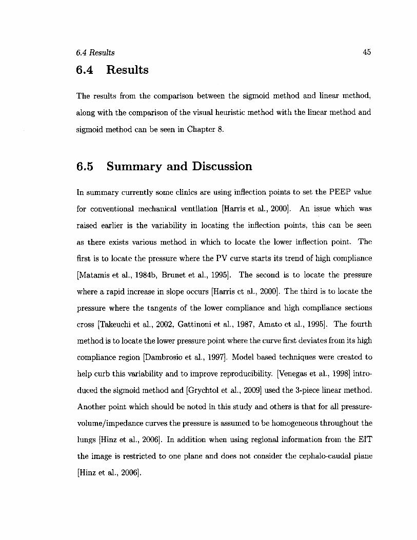
6.4 Results
6.4 Results
45
The results from the comparison between the sigmoid method and linear method,
along with the comparison of the visual heuristic method with the linear method and
sigmoid method can be seen in Chapter 8.
6.5 Summary and Discussion
In summary currently some clinics are using inflection points to set the PEEP value
for conventional mechanical ventilation [Harris et al., 2000]. An issue which was
raised earlier is the variability in locating the inflection points, this can be seen
as there exists various method in which to locate the lower inflection point. The
first is to locate the pressure where the PV curve starts its trend of high compliance
[Matamis et al., 1984b, Brunet et al., 1995]. The second is to locate the pressure
where a rapid increase in slope occurs [Harris et al., 2000]. The third is to locate the
pressure where the tangents of the lower compliance and high compliance sections
cross [Takeuchi et al., 2002, Gattinoni et al., 1987, Amato et al., 1995]. The fourth
method is to locate the lower pressure point where the curve first deviates from its high
compliance region [Dambrosio et al., 1997]. Model based techniques were created to
help curb this variability and to improve reproducibility. [Venegas et al., 1998] intro
duced the sigmoid method and [Grychtol et al., 2009] used the 3-piece linear method.
Another point which should be noted in this study and others is that for all pressure-
volume/impedance curves the pressure is assumed to be homogeneous throughout the
lungs [Hinz et al., 2006]. In addition when using regional information from the EIT
the image is restricted to one plane and does not consider the cephalo-caudal plane
[Hinz et al., 2006].
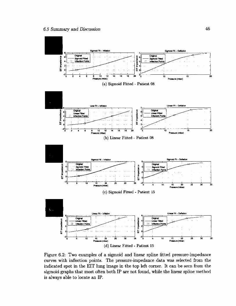
6.5 Summary and Discussion 46
Sigmoid Fit - Inflation Sigmoid Fit - Deflation
Original Sigmoid Fitted
• Inflection Points
Original Sigmoid Fitted
• Inflection Points
i i i i i i i i i i 8 10 12 Pressure (mbar)
Original Sigmoid Fitted Inflection Points
10 15 Pressure (mbar)
(a) Sigmoid Fitted - Patient 08
Unaar Fit - Deflation
Original Linear Fitted
U Inflection Points
Original Linear Fitted
• Inflection Points
8 10 12 14 16 18 20 5 Pressure (mbar)
(b) Linear Fitted - Patient 08 Pressure (mbar)
Sigmoid Fit - Deflation
Original Sigmoid Fitted
• Inflection Points
Original — Sigmoid Fitted J Inflection Points
15 20 Pressure (mbar)
Pressure (mbar)
(c) Sigmoid Fitted - Patient 15
Linear Fit - Inflation
Original Linear Fitted
n Inflection Points
Original Linear Fitted
G Inflection Points
15 20 Pressure (mbar)
15 20 Pressure (mbar)
(d) Linear Fitted - Patient 15
Figure 6.2: Two examples of a sigmoid and linear spline fitted pressure-impedance curves with inflection points. The pressure-impedance data was selected from the indicated spot in the EIT lung image in the top left corner. It can be seen from the sigmoid graphs that most often both IP are not found, while the linear spline method is always able to locate an IP.

Chapter 7
Algorithm Design
This chapter explains the optimal pressure algorithm designed for the use of taking
EIT images and the associated pressure ramp and to calculate the optimal Posi
tive End-Expiatory Pressure (PEEP) to reduce 'bad' (overdistended and collapsed)
lung tissue while maximizing 'good' (well ventilated) lung tissue. The algorithm was
designed and coded in the MATLAB language and was designed to integrate into
preexisting data analysis code from [Pulletz et al., 2011]. The system first calculates
the Inflection Points (IP) from the Pressure-Impedance (PI) graphs, then applies the
IP along with expert knowledge of guided ventilation strategies to create fuzzy mem
bership graphs for a Fuzzy Logic System (FLS), and finally chooses a PEEP. Two
Fuzzy Logic systems were created for comparison, with one using the pressure values
(FSP) of the IP while the other used the EIT values (FSe).
Using the designed algorithm optimal PEEP settings were found on the inflation
and deflation limbs. With multiple patients in the data this chapter will display
examples, results, and overall stats of specific patients or for the entire population.
Using IP as the main source for the membership graphs allowed for past literature
(Chapter 6) to be used in locating an optimal PEEP. The benefits of the approach here

48
is that improvements can be done in parallel. I.E. improving the IP location algorithm
and improvements to the FLS can be done at the same time. [Grychtol et al., 2010]
worked on a similar task but did not use the information provided by the IP and had
more complicated rules in his system. Along with the parallel nature of the design
the ventilation recruitment maneuver was under 2 minutes in length. The last novel
aspect is how regional IP were used when locating the PEEP.
The algorithm is designed into four stages. The first being the locating of the
inflection points. The second is the fuzzification. The third is the premise calculation
and fourth is defuzzification and optimization (Fig. 7.1).
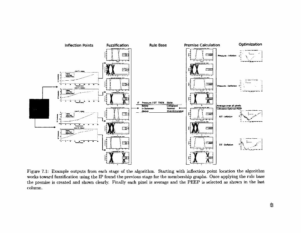
Inflection Points Fuzzification Rule Base Premise Calculation Optimization
Collapsed Normal • Overdistended
Calculate Optimal PEEP
Err - inflation
EIT • Deflation
Figure 7.1: Example outputs from each stage of the algorithm. Starting with inflection point location the algorithm works toward fuzzification using the IP found the previous stage for the membership graphs. Once applying the rule base the premise is created and shown clearly. Finally each pixel is average and the PEEP is selected as shown in the last column.

7.1 Inflection Point Calculation
7.1 Inflection Point Calculation
50
To create the Fuzzy Logic system, regional inflection points were used within the
membership graphs. In order to calculate the inflection points the pressure ramp
and EIT images were first split into two sections: a) inflation limb and b) deflation
limb. Details on the pre-analysis are discussed in Chapter 4.2.3. From here each
pixel within the ROI was fitted to a three-piece linear spline in the partitioned least
squares sense and the IP located. Fig. 7.1 shows an example of the expected output.
The three-piece linear spline algorithm computes the piecewise linear least squares
spline with optimized internal breakpoints. It uses a partitioned least squares for the
parameter estimation and was coded by [D'Errico, 2011]. Initial breakpoint values
used for the linear fit were equally spaced value ranging from the lowest to highest
pressure. From here the matrix A and b were set to solve the inequalities in (7.1).
In (7.1) all inequalities, except Ax < b were not used. The three constraints which
made up A and b are listed below. Where Xin is the input data on the x-axis. a is the
second break point, b is the third break point, with the first and fourth break point
being the min and max of the Xin data and lmin is the minimum length of each line
segment.
1. a > lmin "1"
2. b d > lmin
3. b ^ lmin
(7.1) represents the constraints for the minimization where c(x) and ceq(x) are
non-linear functions which output a vector, x is a vector of the unknown parameters.
A and Aeq are a set of linear equations with inequalities/equalities in b and beq. Finally
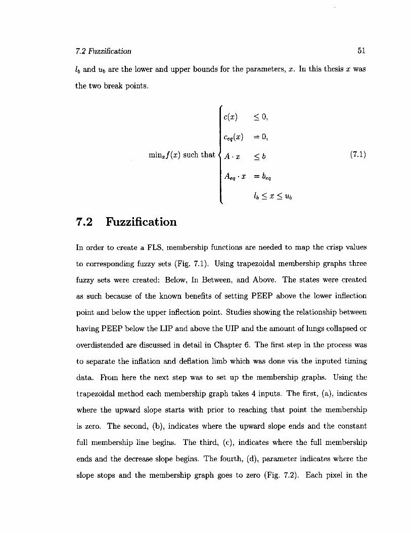
51
In this thesis x was
(7.1)
7.2 Fuzzification
In order to create a FLS, membership functions are needed to map the crisp values
to corresponding fuzzy sets (Fig. 7.1). Using trapezoidal membership graphs three
fuzzy sets were created: Below, In Between, and Above. The states were created
as such because of the known benefits of setting PEEP above the lower inflection
point and below the upper inflection point. Studies showing the relationship between
having PEEP below the LIP and above the UIP and the amount of lungs collapsed or
overdistended are discussed in detail in Chapter 6. The first step in the process was
to separate the inflation and deflation limb which was done via the inputed timing
data. From here the next step was to set up the membership graphs. Using the
trapezoidal method each membership graph takes 4 inputs. The first, (a), indicates
where the upward slope starts with prior to reaching that point the membership
is zero. The second, (b), indicates where the upward slope ends and the constant
full membership line begins. The third, (c), indicates where the full membership
ends and the decrease slope begins. The fourth, (d), parameter indicates where the
slope stops and the membership graph goes to zero (Fig. 7.2). Each pixel in the
7.2 Fuzzification
lb and Ub are the lower and upper bounds for the parameters, x.
the two break points.
minx/(x) such that <
c(x) < 0 ,
Ceq(x) = 0 ,
A • x < b
Aeq ' X = beq
l b < x < u b
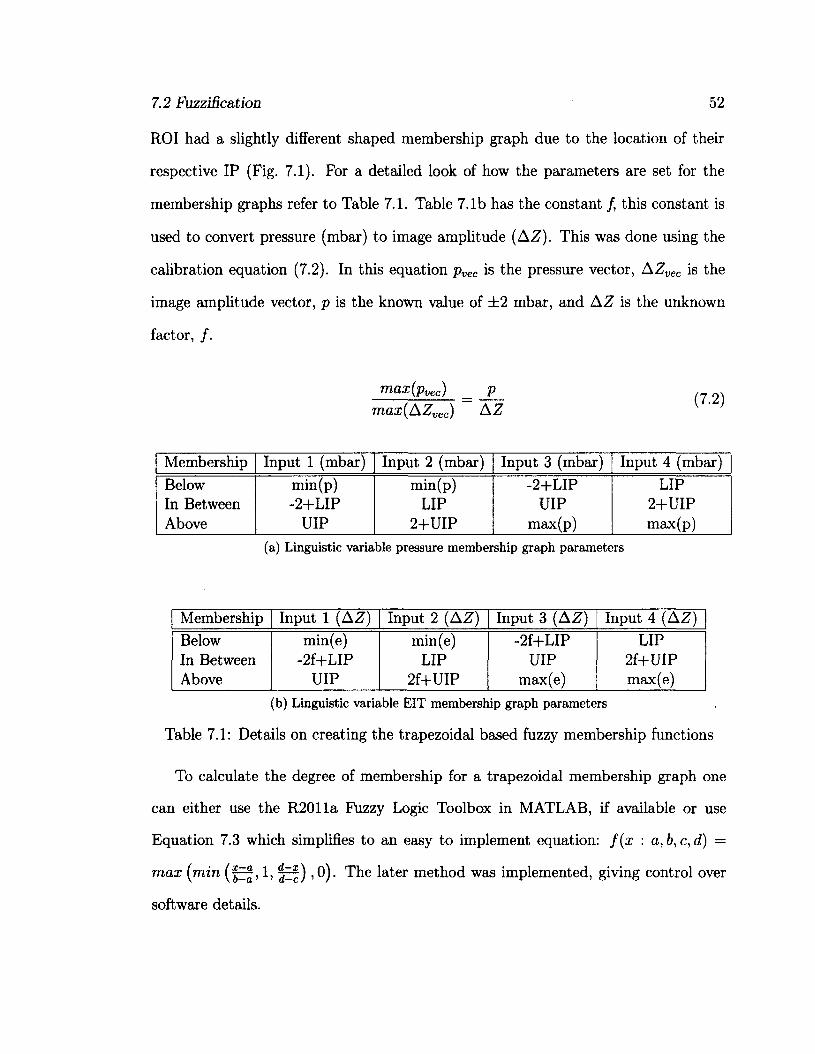
7.2 Fuzzification 52
ROI had a slightly different shaped membership graph due to the location of their
respective IP (Fig. 7.1). For a detailed look of how the parameters are set for the
membership graphs refer to Table 7.1. Table 7.1b has the constant /, this constant is
used to convert pressure (mbar) to image amplitude (AZ). This was done using the
calibration equation (7.2). In this equation pvec is the pressure vector, AZvec is the
image amplitude vector, p is the known value of ±2 mbar, and AZ is the unknown
factor, /.
max(pvec) _ p
max(AZvec) A Z
Membership Input 1 (mbar) Input 2 (mbar) Input 3 (mbar) Input 4 (mbar) Below min(p) min(p) -2+LIP LIP In Between -2+LIP LIP UIP 2+UIP Above UIP 2+UIP max(p) max(p)
(a) Linguistic variable pressure membership graph parameters
Membership Input 1 (A Z) Input 2 (AZ) Input 3 (AZ) Input 4 (AZ)
Below In Between Above
min(e) -2f+LIP
UIP
min(e) LIP
2f+UIP
-2f+LIP UIP
max(e)
LIP 2f+UIP max(e)
(b) Linguistic variable EIT membership graph parameters
Table 7.1: Details on creating the trapezoidal based fuzzy membership functions
To calculate the degree of membership for a trapezoidal membership graph one
can either use the R2011a Fuzzy Logic Toolbox in MATLAB, if available or use
E q u a t i o n 7 . 3 w h i c h s i m p l i f i e s t o a n e a s y t o i m p l e m e n t e q u a t i o n : f ( x : a , b , c , d ) =
max (min (|1, , 0). The later method was implemented, giving control over
software details.
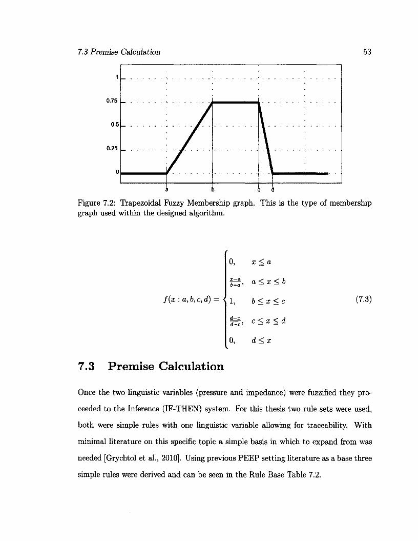
7.3 Premise Calculation 53
0.75
0.25
0.5
0
b c d a
Figure 7.2: Trapezoidal Fuzzy Membership graph. This is the type of membership graph used within the designed algorithm.
0, d < x
7.3 Premise Calculation
Once the two linguistic variables (pressure and impedance) were fuzzified they pro
ceeded to the Inference (IF-THEN) system. For this thesis two rule sets were used,
both were simple rules with one linguistic variable allowing for traceability. With
minimal literature on this specific topic a simple basis in which to expand from was
needed [Grychtol et al., 2010]. Using previous PEEP setting literature as a base three
simple rules were derived and can be seen in the Rule Base Table 7.2.
0, x < a
f - f , a < x < b o—a' — —
f ( x : a , b , c , d ) = i 1 b < x < c (7.3)
f c f ' c < x < d
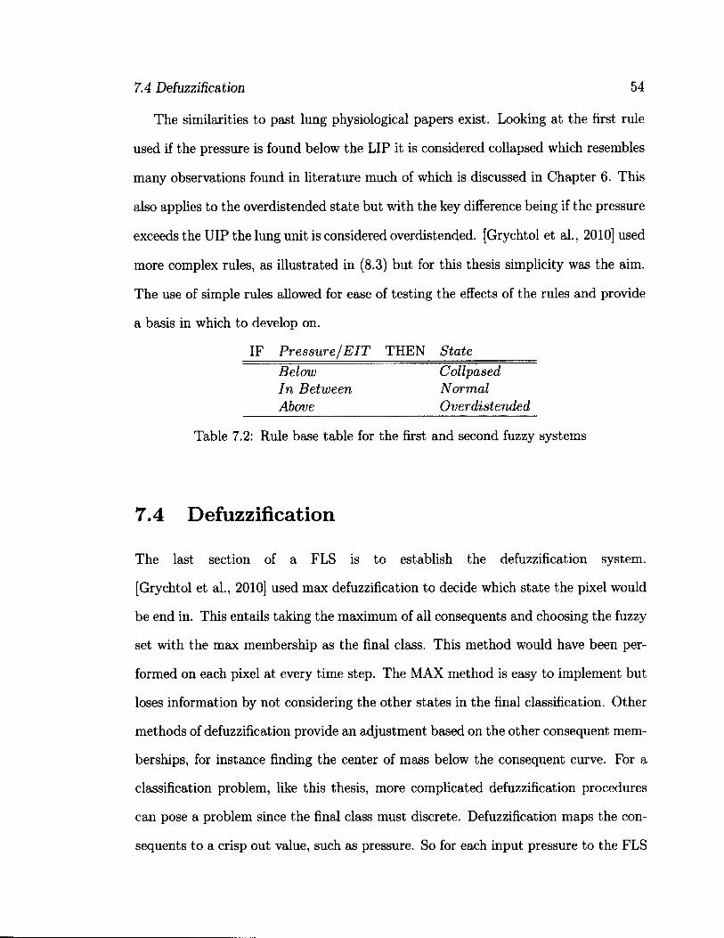
7.4 Defuzzification 54
The similarities to past lung physiological papers exist. Looking at the first rule
used if the pressure is found below the LIP it is considered collapsed which resembles
many observations found in literature much of which is discussed in Chapter 6. This
also applies to the overdistended state but with the key difference being if the pressure
exceeds the UIP the lung unit is considered overdistended. [Grychtol et al, 2010] used
more complex rules, as illustrated in (8.3) but for this thesis simplicity was the aim.
The use of simple rules allowed for ease of testing the effects of the rules and provide
a basis in which to develop on.
7.4 Defuzzification
The last section of a FLS is to establish the defuzzification system.
[Grychtol et al., 2010] used max defuzzification to decide which state the pixel would
be end in. This entails taking the maximum of all consequents and choosing the fuzzy
set with the max membership as the final class. This method would have been per
formed on each pixel at every time step. The MAX method is easy to implement but
loses information by not considering the other states in the final classification. Other
methods of defuzzification provide an adjustment based on the other consequent mem
berships, for instance finding the center of mass below the consequent curve. For a
classification problem, like this thesis, more complicated defuzzification procedures
can pose a problem since the final class must discrete. Defuzzification maps the con
sequents to a crisp out value, such as pressure. So for each input pressure to the FLS
IF Pressure/EIT THEN State
Below In Between Above
Collpased Normal Overdistended
Table 7.2: Rule base table for the first and second fuzzy systems

7.5 Summary and Discussion 55
the output would also be a pressure. This would work fine for a control system but
for our purpose, classification, we don't have a single input measurement but rather
we are looking for an optimal PEEP from an entire range of pressures. For this thesis
the MAX method was not used since the membership degree was kept to use all the
information available in the pressure optimization.
The pressure optimization was done by categorizing each of the consequents into
a 'good' and 'bad' category. The 'good' category consisted of units within the normal
consequent state while the 'bad' category consisted of units within the collapsed and
overdistended consequent states. From here the sum for all the pixels were taken with
the logic that a single pressure must be selected for the entire ventilation system. This
leads to working with two 1-D vectors with the x-axis being the index for the optimal
pressure. This is shown in Fig. 7.1 as the last section in the diagram, Optimization.
To find the optimal index the bad states was subtracted from the good states and
the global max was found of the resulting curve. For examples refer to Fig. 7.1.
7.5 Summary and Discussion
In summary this algorithm was designed to use the regional information from an EIT
system to locate regional IP with the ultimate means of locating an optimal PEEP
pressure. The steps taken were to first fit the PI graphs to a three-piece linear spline.
From here the inflection points were taken as the location of the breakpoints where
the pressure and impedance change values were used to create membership graph
for two FLS. The membership graphs map the pressure and impedance change to
3 fuzzy sets: Below, In Between, and Above. The significance of these fuzzy sets
are that they ensure the that optimal PEEP is found somewhere between the two
inflection points. The significance of this point is discussed in Chapter 6. Once

7.5 Summary and Discussion 56
fuzzified the fuzzy sets are used in IF-THEN rules to create 3 conclusions: Collapsed,
Normal, and Overdistended. The rules for each system can be seen in Table 7.2.
With the conclusions now established for each pixel they are put into 'good' and
'bad' categorizes. The 'good' category consists of pixels within the Normal conclusion
with the 'bad' category consisting of the Collapsed and Overdistended conclusions.
From here the sum of the membership values for the two categories is done and the
difference between 'good' and 'bad' is taken to find the maximum of the difference.
The max location signifies the index for the optimal pressure. Finding the best PEEP
is a matter of using the index in the pressure vector.
The system created here is a large first step into using both EIT and Fuzzy Logic
for the purpose of PEEP adjustment.

Chapter 8
Results and Analysis
This chapter explains the results from the algorithm described in Chapter 7. The
data used for comparison and analysis is described in Chapter 4. This chapter goes
through a comparative analysis of the linear and sigmoid methods, the linear and
visual heuristic methods, the sigmoid and visual heuristic methods, analysis of the
membership graphs, and finally an analysis of the PEEP selection.
8.1 Inflection Points
This section compares the inflection points (IP) using the linear method, the sigmoid
method, and the visual heuristic method.
8.1.1 Inflection Points for Individual Algorithms
To find the regional IP a 3-piece linear spline [Grychtol et al., 2009] was used with
optimal breakpoint location [D'Errico, 2011]. The algorithm is described in Chapter
7. When comparing LIP found between control and ALI patients, a noticeable dif
ference in value was found with the ALI patients having an average LIP of 10.7146
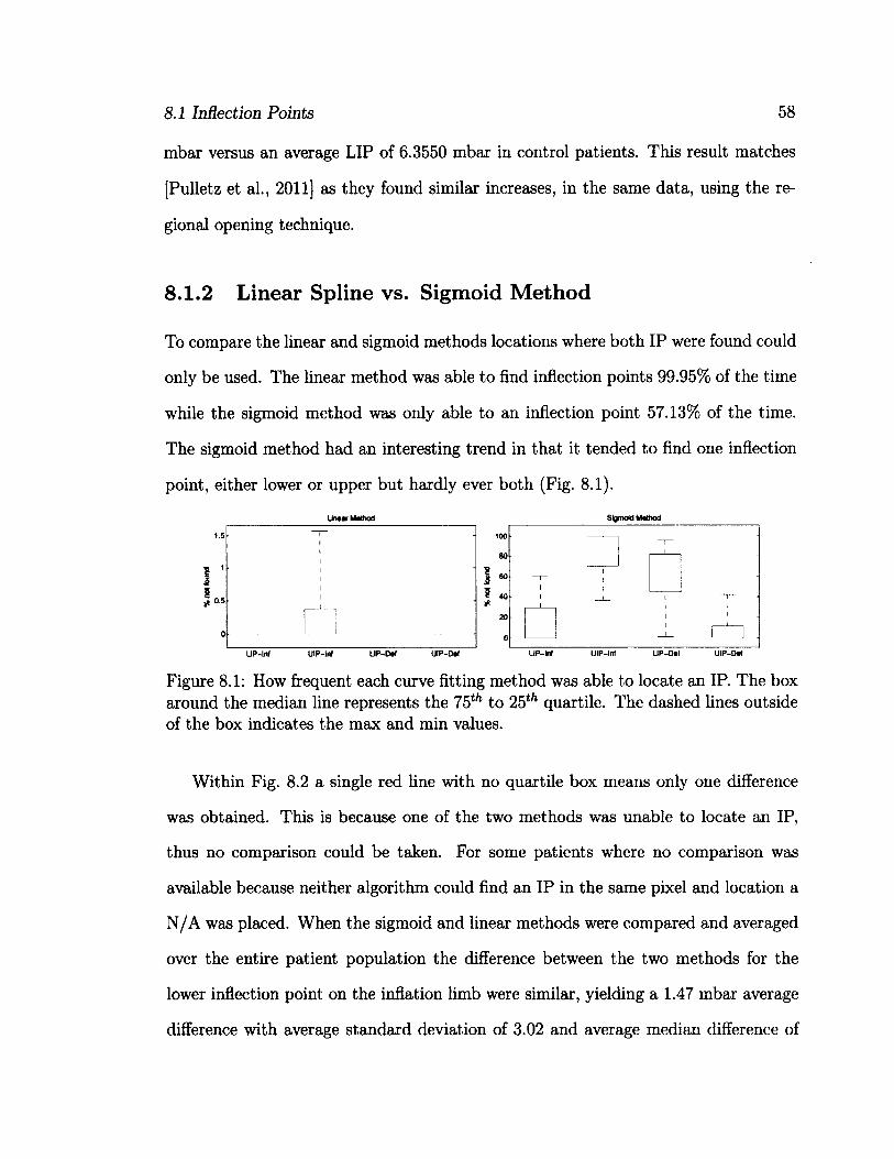
8.1 Inflection Points 58
mbar versus an average LIP of 6.3550 mbar in control patients. This result matches
[Pulletz et al., 2011] as they found similar increases, in the same data, using the re
gional opening technique.
8.1.2 Linear Spline vs. Sigmoid Method
To compare the linear and sigmoid methods locations where both IP were found could
only be used. The linear method was able to find inflection points 99.95% of the time
while the sigmoid method was only able to an inflection point 57.13% of the time.
The sigmoid method had an interesting trend in that it tended to find one inflection
point, either lower or upper but hardly ever both (Fig. 8.1).
Sigmoid Method
Figure 8.1: How frequent each curve fitting method was able to locate an IP. The box around the median line represents the 75th to 25th quartile. The dashed lines outside of the box indicates the max and min values.
Within Fig. 8.2 a single red line with no quartile box means only one difference
was obtained. This is because one of the two methods was unable to locate an IP,
thus no comparison could be taken. For some patients where no comparison was
available because neither algorithm could find an IP in the same pixel and location a
N/A was placed. When the sigmoid and linear methods were compared and averaged
over the entire patient population the difference between the two methods for the
lower inflection point on the inflation limb were similar, yielding a 1.47 mbar average
difference with average standard deviation of 3.02 and average median difference of
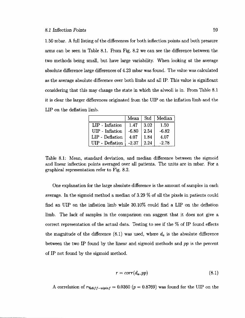
8.1 Inflection Points 59
1.50 mbar. A full listing of the differences for both inflection points and both pressure
arms can be seen in Table 8.1. From Fig. 8.2 we can see the difference between the
two methods being small, but have large variability. When looking at the average
absolute difference large differences of 4.23 mbar was found. The value was calculated
as the average absolute difference over both limbs and all IP. This value is significant
considering that this may change the state in which the alveoli is in. From Table 8.1
it is clear the larger differences originated from the UIP on the inflation limb and the
LIP on the deflation limb.
Mean Std Median LIP - Inflation 1.47 3.02 1.50 UIP- Inflation -6.80 2.54 -6.82 LIP - Deflation 4.07 1.84 4.07 UIP- Deflation -2.37 2.24 -2.78
Table 8.1: Mean, standard deviation, and median difference between the sigmoid and linear inflection points averaged over all patients. The units are in mbar. For a graphical representation refer to Fig. 8.2.
One explanation for the large absolute difference is the amount of samples in each
average. In the sigmoid method a median of 3.29 % of all the pixels in patients could
find an UIP on the inflation limb while 30.10% could find a LIP on the deflation
limb. The lack of samples in the comparison can suggest that it does not give a
correct representation of the actual data. Testing to see if the % of IP found effects
the magnitude of the difference (8.1) was used, where da is the absolute difference
between the two IP found by the linear and sigmoid methods and pp is the percent
of IP not found by the sigmoid method.
A correlation of r%diff-uipinf
r = corr(da,pp) (8.1)
= 0.0360 (p = 0.8769) was found for the UIP on the
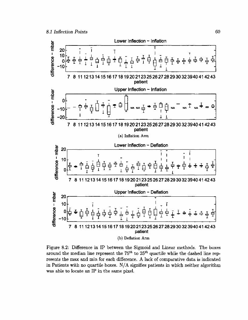
8.1 Inflection Points 60
Lower Inflection - Inflation
20
» 10
£ 0
I -10
7 8 11 1213141516171819202123252627282930323940414243 patient
Upper Inflection - Inflation
N/A N/A
<£> -20
7 8 11 1213141516171819202123252627282930323940414243 patient
(a) Inflation Arm
Lower Inflection - Deflation
7 8 11 1213141516171819202123252627282930323940414243 patient
Upper Inflection - Deflation
7 8 11 1213141516171819202123252627282930323940414243 patient
(b) Deflation Arm
Figure 8.2: Difference in IP between the Sigmoid and Linear methods. The boxes around the median line represent the 75th to 25th quartile while the dashed line represents the max and min for each difference. A lack of comparative data is indicated in Patients with no quartile boxes. N/A signifies patients in which neither algorithm was able to locate an IP in the same pixel.
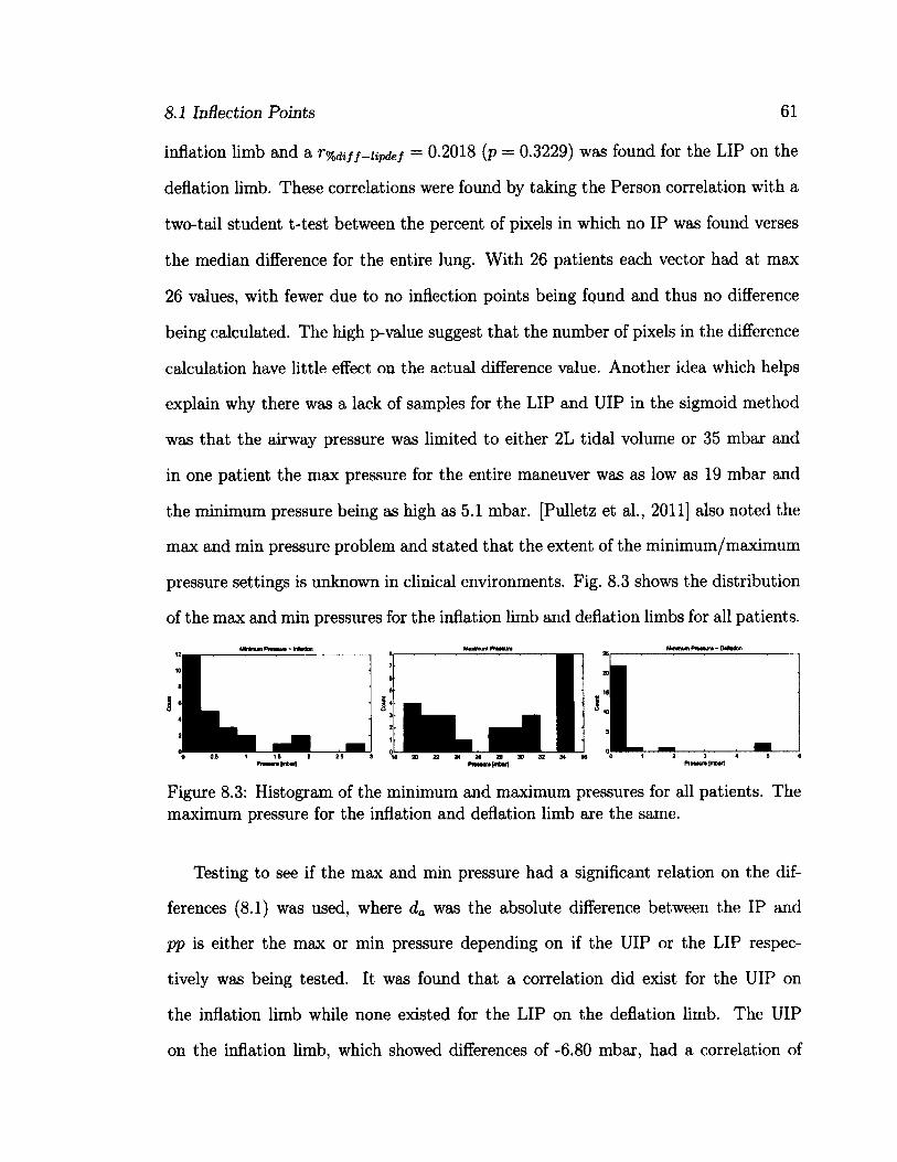
8.1 Inflection Points 61
inflation limb and a r% d i f f^ii p d e f = 0.2018 (p = 0.3229) was found for the LIP on the
deflation limb. These correlations were found by taking the Person correlation with a
two-tail student t-test between the percent of pixels in which no IP was found verses
the median difference for the entire lung. With 26 patients each vector had at max
26 values, with fewer due to no inflection points being found and thus no difference
being calculated. The high p-value suggest that the number of pixels in the difference
calculation have little effect on the actual difference value. Another idea which helps
explain why there was a lack of samples for the LIP and UIP in the sigmoid method
was that the airway pressure was limited to either 2L tidal volume or 35 mbar and
in one patient the max pressure for the entire maneuver was as low as 19 mbar and
the minimum pressure being as high as 5.1 mbar. [Pulletz et al., 2011] also noted the
max and min pressure problem and stated that the extent of the minimum/maximum
pressure settings is unknown in clinical environments. Fig. 8.3 shows the distribution
of the max and min pressures for the inflation limb and deflation limbs for all patients.
8 2 0 2 2 2 4 2 6 2 8 ) 0 3 2 3 4 9 6
Figure 8.3: Histogram of the minimum and maximum pressures for all patients. The maximum pressure for the inflation and deflation limb are the same.
Testing to see if the max and min pressure had a significant relation on the dif
ferences (8.1) was used, where da was the absolute difference between the IP and
pp is either the max or min pressure depending on if the UIP or the LIP respec
tively was being tested. It was found that a correlation did exist for the UIP on
the inflation limb while none existed for the LIP on the deflation limb. The UIP
on the inflation limb, which showed differences of -6.80 mbar, had a correlation of
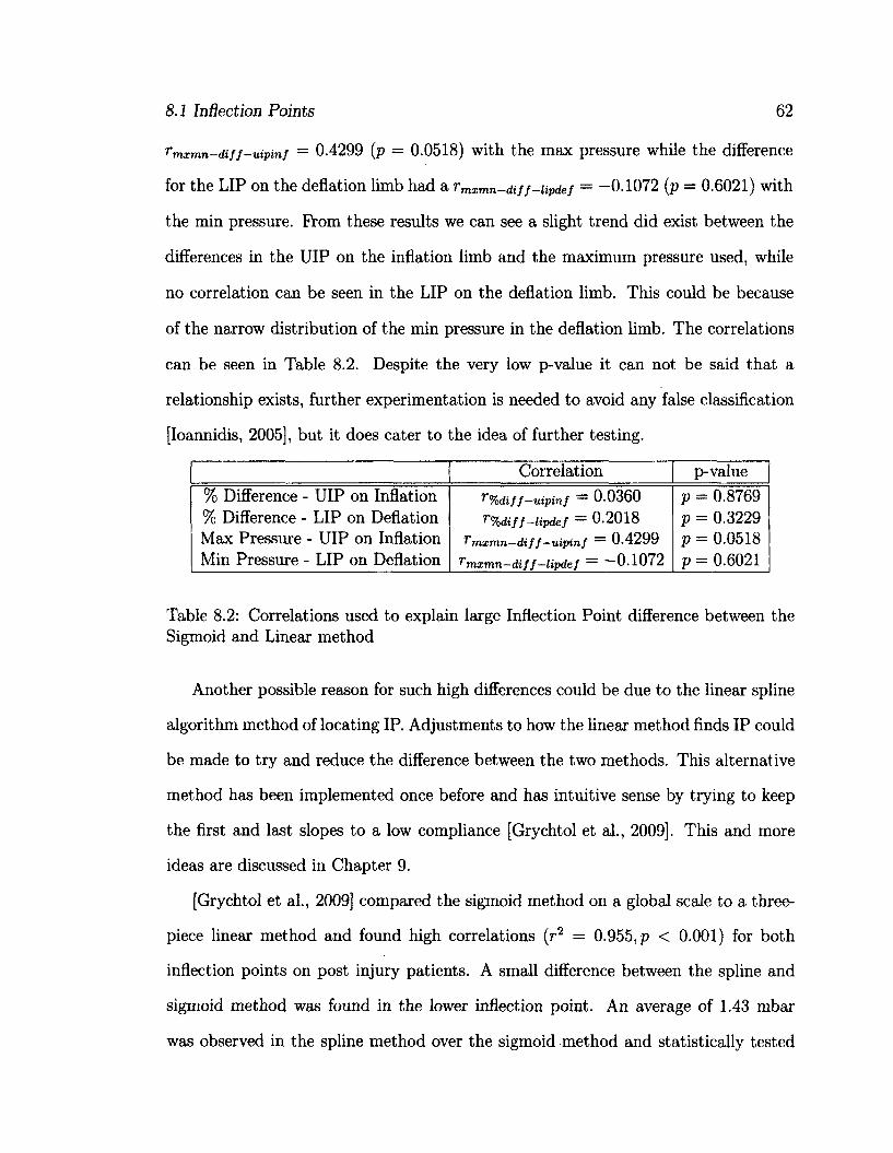
8.1 Inflection Points 62
Tmxmn—diff—uipinf = 0.4299 (p = 0.0518) with the max pressure while the difference
for the LIP on the deflation limb had a rmxrnn-diff-iipdef = -0.1072 (p = 0.6021) with
the min pressure. Prom these results we can see a slight trend did exist between the
differences in the UIP on the inflation limb and the maximum pressure used, while
no correlation can be seen in the LIP on the deflation limb. This could be because
of the narrow distribution of the min pressure in the deflation limb. The correlations
can be seen in Table 8.2. Despite the very low p-value it can not be said that a
relationship exists, further experimentation is needed to avoid any false classification
[Ioannidis, 2005], but it does cater to the idea of further testing.
Correlation p-value % Difference - UIP on Inflation % Difference - LIP on Deflation Max Pressure - UIP on Inflation Min Pressure - LIP on Deflation
V%diff—uipinf ~ 0.0360 T%dif f—lipdef 0.2018
f mxmn—dif f—uipinf = 0.4299 ^mxmn—diff—lipdef = 0.1072
p = 0.8769 p = 0.3229 p = 0.0518 p = 0.6021
Table 8.2: Correlations used to explain large Inflection Point difference between the Sigmoid and Linear method
Another possible reason for such high differences could be due to the linear spline
algorithm method of locating IP. Adjustments to how the linear method finds IP could
be made to try and reduce the difference between the two methods. This alternative
method has been implemented once before and has intuitive sense by trying to keep
the first and last slopes to a low compliance [Grychtol et al., 2009]. This and more
ideas are discussed in Chapter 9.
[Grychtol et al., 2009] compared the sigmoid method on a global scale to a three-
piece linear method and found high correlations (r2 = 0.955, p < 0.001) for both
inflection points on post injury patients. A small difference between the spline and
sigmoid method was found in the lower inflection point. An average of 1.43 mbar
was observed in the spline method over the sigmoid method and statistically tested

8.1 Inflection Points 63
with a paired sample T-test. [Grychtol et al., 2009]s result matches closely with the
difference found in this thesis. In this thesis a 1.47 mbar average difference between
the linear spline and sigmoid method was found.
Overall the difference between the IPs found by the two methods were similar
and match previous results [Grychtol et al., 2009]. A major improvement with the
linear method compared to the sigmoid method is the consistency in finding IPs. As
mentioned earlier the linear method was able to locate an IP 99.95 % while the sigmoid
method was only able to locate IPs 57.13% of the time. The consistency found in
the linear method allows for repeatable results over multiple experiments. The linear
methods similarity to manual curve fitting also makes it a great fit for hospitals as
clinicians will be familiar with workings and understand the results better then using
the sigmoid method.
8.1.3 Linear and Sigmoid vs. Visual Heuristics
In this thesis we tested four pixels from each patient and asked five volunteers to
fit three linear segments to the data. All volunteers except one had an Engineering
background with the other having an English major background. The location of the
inflection points were the points where the two lateral line segments intersected the
median. An example of what each participant had to do is illustrated in (Fig. 8.4).
The provided instructions were to fit the data in an optimal manner with three line
segments. Each participant worked with both the inflation and deflation arms of the
recruitment maneuver thus fitting eight pressure-impedance (PI) curves per patient.
The experiment was designed in such a way that each person was only given one
chance to place an IP thus medians over the participants were taken to help reduce
the effects of a misplaced IP. It should be noted that each participant fitted the same
PI curves providing continuity between participants and allowing for stats to taken
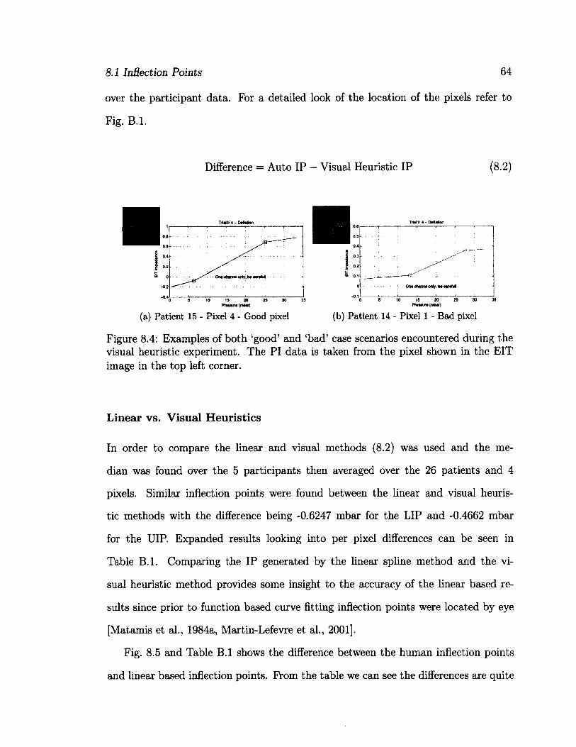
8.1 Inflection Points
over the participant data.
Fig. B.l.
64
For a detailed look of the location of the pixels refer to
Difference = Auto IP - Visual Heuristic IP (8.2)
Prwaur* (mbar) Pwxuf (mbaf)
(a) Patient 15 - Pixel 4 - Good pixel (b) Patient 14 - Pixel 1 - Bad pixel
Figure 8.4: Examples of both 'good' and 'bad' case scenarios encountered during the visual heuristic experiment. The PI data is taken from the pixel shown in the EIT image in the top left corner.
Linear vs. Visual Heuristics
In order to compare the linear and visual methods (8.2) was used and the me
dian was found over the 5 participants then averaged over the 26 patients and 4
pixels. Similar inflection points were found between the linear and visual heuris
tic methods with the difference being -0.6247 mbar for the LIP and -0.4662 mbar
for the UIP. Expanded results looking into per pixel differences can be seen in
Table B.l. Comparing the IP generated by the linear spline method and the vi
sual heuristic method provides some insight to the accuracy of the linear based re
sults since prior to function based curve fitting inflection points were located by eye
[Matamis et al., 1984a, Martin-Lefevre et al., 2001].
Fig. 8.5 and Table B.l shows the difference between the human inflection points
and linear based inflection points. From the table we can see the differences are quite
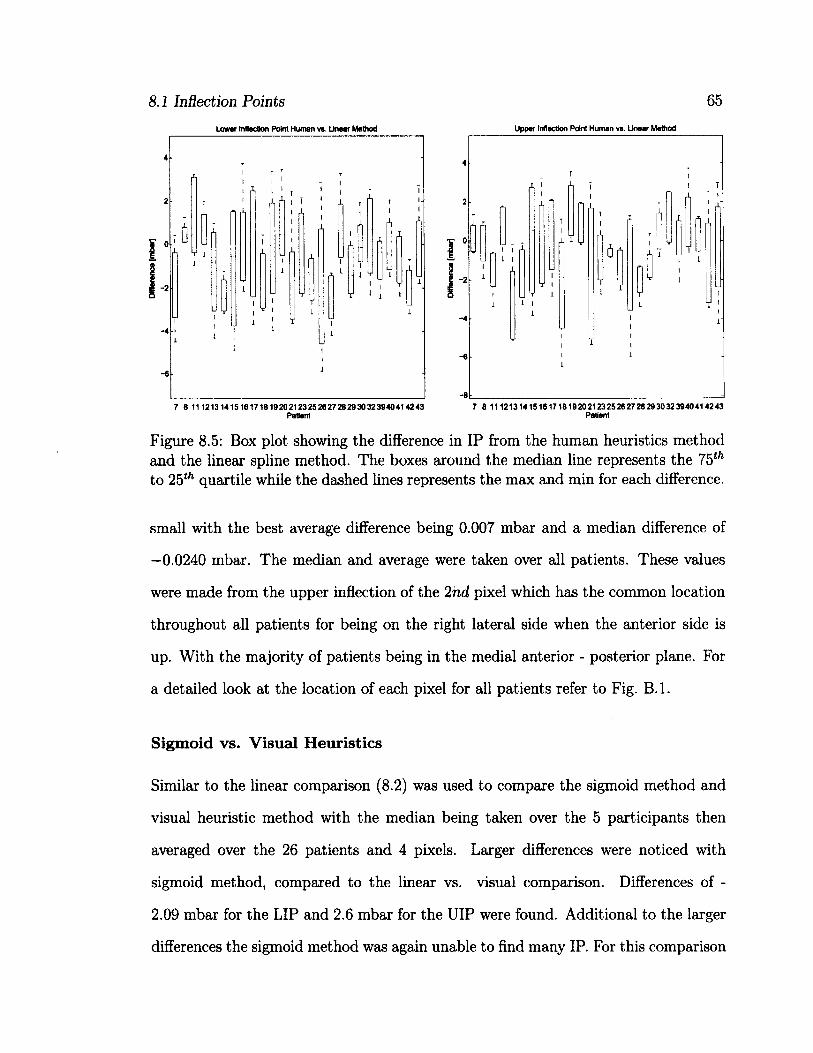
8.1 Inflection Points 65
Lower Inflection Point Human vs. Linear Method Upper Inflection Point Human vs. Linear Method
7 8 111213141516171819202123252627262930323940414243 Patient
7 8 111213141516171819202123252627282930323940414243 Patient
Figure 8.5: Box plot showing the difference in IP from the human heuristics method and the linear spline method. The boxes around the median line represents the 75th
to 25th quartile while the dashed lines represents the max and min for each difference.
small with the best average difference being 0.007 mbar and a median difference of
—0.0240 mbar. The median and average were taken over all patients. These values
were made from the upper inflection of the 2nd pixel which has the common location
throughout all patients for being on the right lateral side when the anterior side is
up. With the majority of patients being in the medial anterior - posterior plane. For
a detailed look at the location of each pixel for all patients refer to Fig. B.l.
Sigmoid vs. Visual Heuristics
Similar to the linear comparison (8.2) was used to compare the sigmoid method and
visual heuristic method with the median being taken over the 5 participants then
averaged over the 26 patients and 4 pixels. Larger differences were noticed with
sigmoid method, compared to the linear vs. visual comparison. Differences of -
2.09 mbar for the LIP and 2.6 mbar for the UIP were found. Additional to the larger
differences the sigmoid method was again unable to find many IP. For this comparison
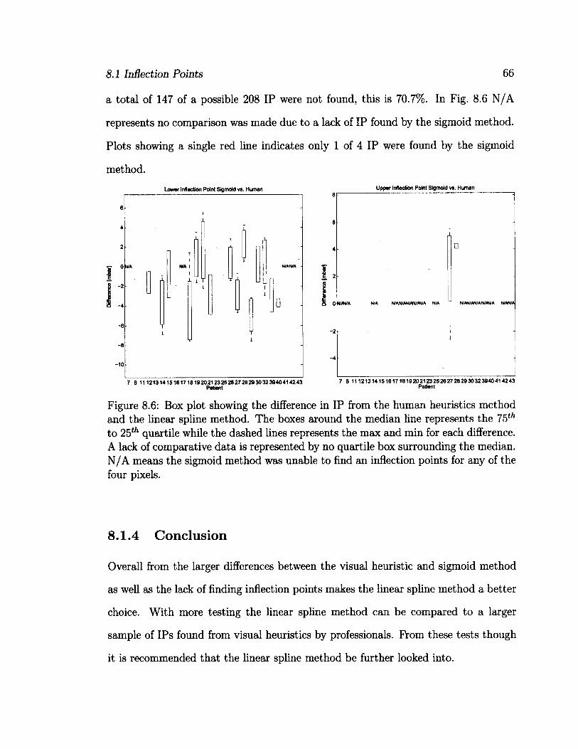
8.1 Inflection Points 66
a total of 147 of a possible 208 IP were not found, this is 70.7%. In Fig. 8.6 N/A
represents no comparison was made due to a lack of IP found by the sigmoid method.
Plots showing a single red line indicates only 1 of 4 IP were found by the sigmoid
method.
Lower Inflection Point Sigmoid vs. Human Upper Inflection Point Sigmoid vs. Human
WAVA N/A N/AN/AN/AfMN/A N/A N/AN/AN/AN/A4/A N/AN/A
7 8 111213141516171819202123252627282930323940414243 Patient
7 8 111213141516171819202123252627282930323940414243 P8tient
Figure 8.6: Box plot showing the difference in IP from the human heuristics method and the linear spline method. The boxes around the median line represents the 75th
to 25th quartile while the dashed lines represents the max and min for each difference. A lack of comparative data is represented by no quartile box surrounding the median. N/A means the sigmoid method was unable to find an inflection points for any of the four pixels.
8.1.4 Conclusion
Overall from the larger differences between the visual heuristic and sigmoid method
as well as the lack of finding inflection points makes the linear spline method a better
choice. With more testing the linear spline method can be compared to a larger
sample of IPs found from visual heuristics by professionals. From these tests though
it is recommended that the linear spline method be further looked into.
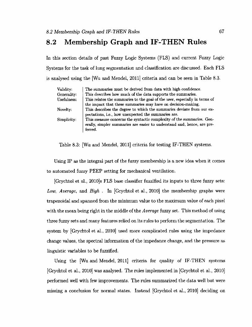
8.2 Membership Graph and IF-THEN Rules 67
8.2 Membership Graph and IF-THEN Rules
In this section details of past Fuzzy Logic Systems (FLS) and current Fuzzy Logic
Systems for the task of lung segmentation and classification are discussed. Each FLS
is analysed using the [Wu and Mendel, 2011] criteria and can be seen in Table 8.3.
Validity: Generality: Usefulness:
Novelty:
Simplicity:
The summaries must be derived from data with high confidence. This describes how much of the data supports the summaries. This relates the summaries to the goal of the user, especially in terms of the impact that these summaries may have on decision-making. This describes the degree to which the summaries deviate from our expectations, i.e., how unexpected the summaries are. This measure concerns the syntactic complexity of the summaries. Generally, simpler summaries are easier to understand and, hence, are preferred.
Table 8.3: [Wu and Mendel, 2011] criteria for testing IF-THEN systems.
Using IP as the integral part of the fuzzy membership is a new idea when it comes
to automated fuzzy PEEP setting for mechanical ventilation.
[Grychtol et al., 2010]s FLS base classifier fuzzified its inputs to three fuzzy sets:
Low, Average, and High . In [Grychtol et al., 2010] the membership graphs were
trapezoidal and spanned from the minimum value to the maximum value of each pixel
with the mean being right in the middle of the Average fuzzy set. This method of using
three fuzzy sets and many features relied on its rules to perform the segmentation. The
system by [Grychtol et al., 2010] used more complicated rules using the impedance
change values, the spectral information of the impedance change, and the pressure as
linguistic variables to be fuzzified.
Using the [Wu and Mendel, 2011] criteria for quality of IF-THEN systems
[Grychtol et al., 2010] was analysed. The rules implemented in [Grychtol et al., 2010]
performed well with few improvements. The rules summarized the data well but were
missing a conclusion for normal states. Instead [Grychtol et al., 2010] deciding on

8.2 Membership Graph and IF-THEN Rules 68
using the transition states such as; Collapsing, Opening, Recovering and Overdis-
tending. The implemented rules were useful in achieving the goal of classification
and do provide novelty; but, when simplicity is a concern, this set of rules are quite
complicated. An example of one of the rules in [Grychtol et al., 2010] can be seen
below.
Opening(n) = (feit(n) = Lo) fl (feit(n — 1) = Lo) fi (sgn(Afeit(n)) = Hi) (8.3)
H ( sgn (Aa(n ) ) = Lo) fl (sgn(Ap) = Hi)
Similar to [Grychtol et al., 2010] this thesis has satisfied many of
[Wu and Mendel, 2011] criteria. Validity: The rules in the FLS system were
very closely tied to the data as they used the inflection points and knowledge of how
PEEP was set in previous studies to create the membership which intern lead to
the rules. Generality: This criteria was harder to asses as no hard validation data
was available. While the data used created the membership graphs and rule base
it can not be said if the data supports the truth of the rules. Since the IP were an
integral part in the creation of the membership graphs if the IP were miscalculated
the error would propagate into the FLS thus determining where the error originates
impertinent. Usefulness: The rules in this FLS were extremely useful with no
redundant or useless rules. Novelty: The rule base is novel as including the IP in a
FLS has not been done before but the rules were largely based on knowledge attained
from previous global based PEEP settings. An overview of past PEEP settings
are discussed in Chapter 6. Simplicity: The rule base in this study were extremely
simple.
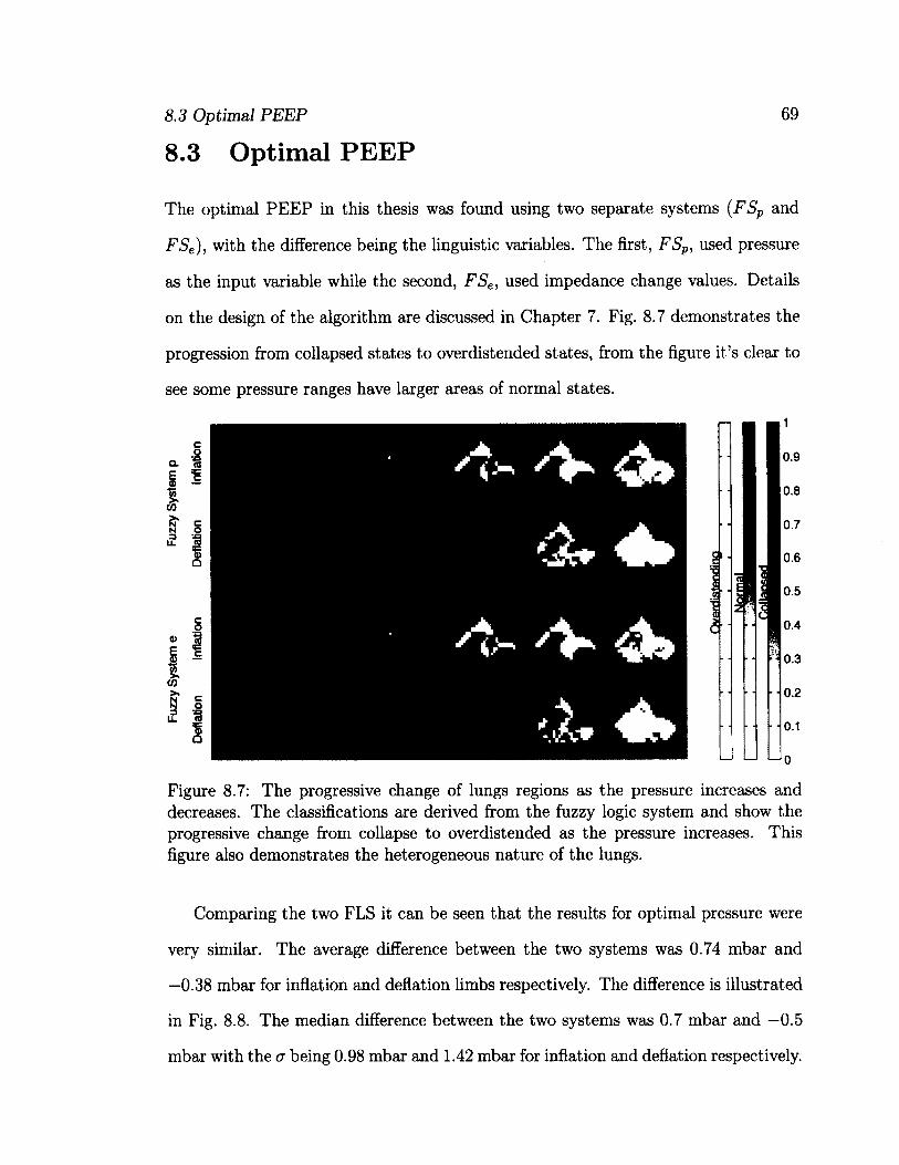
8.3 Optimal PEEP
8.3 Optimal PEEP
69
The optimal PEEP in this thesis was found using two separate systems (FSP and
FSe), with the difference being the linguistic variables. The first, FSP, used pressure
as the input variable while the second, FSe, used impedance change values. Details
on the design of the algorithm are discussed in Chapter 7. Fig. 8.7 demonstrates the
progression from collapsed states to overdistended states, from the figure it's clear to
see some pressure ranges have larger areas of normal states.
Figure 8.7: The progressive change of lungs regions as the pressure increases and decreases. The classifications are derived from the fuzzy logic system and show the progressive change from collapse to overdistended as the pressure increases. This figure also demonstrates the heterogeneous nature of the lungs.
Comparing the two FLS it can be seen that the results for optimal pressure were
very similar. The average difference between the two systems was 0.74 mbar and
—0.38 mbar for inflation and deflation limbs respectively. The difference is illustrated
in Fig. 8.8. The median difference between the two systems was 0.7 mbar and —0.5
mbar with the <r being 0.98 mbar and 1.42 mbar for inflation and deflation respectively.
o
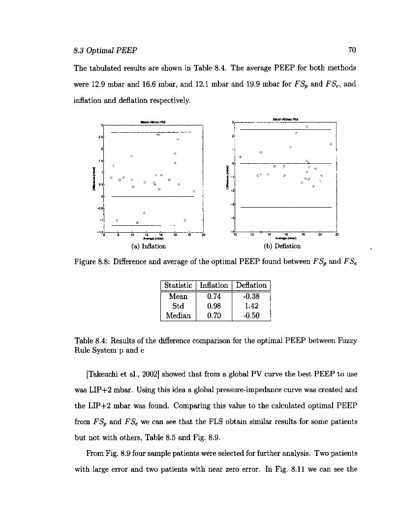
8.3 Optimal PEEP 70
The tabulated results are shown in Table 8.4. The average PEEP for both methods
were 12.9 mbar and 16.6 mbar, and 12.1 mbar and 19.9 mbar for FSP and FSe, and
inflation and deflation respectively.
Plot
2.5
-0,5
-1.5 e 8 10 12 14 18 18 20
Awagi (mbarf 14 16 18 20
Av*rag* [mbar]
(a) Inflation (b) Deflation
Figure 8.8: Difference and average of the optimal PEEP found between FSP and FSe
Statistic Inflation Deflation Mean 0.74 -0.38 Std 0.98 1.42
Median 0.70 -0.50
Table 8.4: Results of the difference comparison for the optimal PEEP between Fuzzy Rule System p and e
[Takeuchi et al., 2002] showed that from a global PV curve the best PEEP to use
was LIP+2 mbar. Using this idea a global pressure-impedance curve was created and
the LIP+2 mbar was found. Comparing this value to the calculated optimal PEEP
from FSP and FSe we can see that the FLS obtain similar results for some patients
but not with others, Table 8.5 and Fig. 8.9.
From Fig. 8.9 four sample patients were selected for further analysis. Two patients
with large error and two patients with near zero error. In Fig. 8.11 we can see the
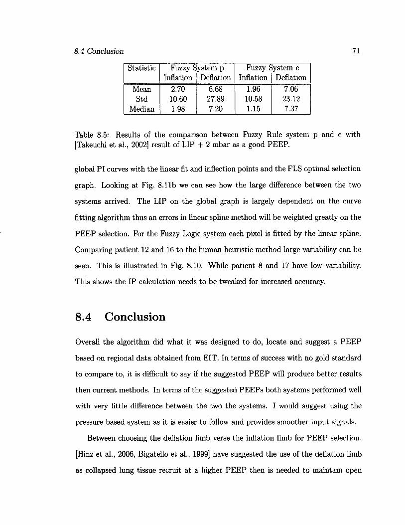
8.4 Conclusion 71
Statistic Fuzzy System p Fuzzy System e Inflation Deflation Inflation Deflation
Mean 2.70 6.68 1.96 7.06 Std 10.60 27.89 10.58 23.12
Median 1.98 7.20 1.15 7.37
Table 8.5: Results of the comparison between Fuzzy Rule system p and e with [Takeuchi et al., 2002] result of LIP + 2 mbar as a good PEEP.
global PI curves with the linear fit and inflection points and the FLS optimal selection
graph. Looking at Fig. 8.11b we can see how the large difference between the two
systems arrived. The LIP on the global graph is largely dependent on the curve
fitting algorithm thus an errors in linear spline method will be weighted greatly on the
PEEP selection. For the Fuzzy Logic system each pixel is fitted by the linear spline.
Comparing patient 12 and 16 to the human heuristic method large variability can be
seen. This is illustrated in Fig. 8.10. While patient 8 and 17 have low variability.
This shows the IP calculation needs to be tweaked for increased accuracy.
8.4 Conclusion
Overall the algorithm did what it was designed to do, locate and suggest a PEEP
based on regional data obtained from EIT. In terms of success with no gold standard
to compare to, it is difficult to say if the suggested PEEP will produce better results
then current methods. In terms of the suggested PEEPs both systems performed well
with very little difference between the two the systems. I would suggest using the
pressure based system as it is easier to follow and provides smoother input signals.
Between choosing the deflation limb verse the inflation limb for PEEP selection.
[Hinz et al., 2006, Bigatello et al., 1999] have suggested the use of the deflation limb
as collapsed lung tissue recruit at a higher PEEP then is needed to maintain open

8.4 Conclusion 72
tissue. In this thesis opposite results were noticed, as shown in Fig. 8.12. This can be
explained since prior to the recruitment maneuver ventilated breathing of the patient
was taking place. This ventilation could have already initially recruited the tissue.
Drawing conclusions from the comparisons it can be said that the linear method for
locating inflection points from pressure-impedance graphs is worth using. The linear
method allows for locating inflection points reliably. It's also easy to understand by
doctors, providing easy to access standards. It also obtained similar results to the
visual heuristic method showing it's accuracy. It also had similar results to that of
the Sigmoid method which is known to be a classical method for locating IP.
The automated PEEP portion of the work also worked well. It was able to suggest
a PEEP using regional IP and knowledge of the use of PEEP and the effect on lung
tissue at various PEEPs. The designed system also has benefit to be used to control
mechanical ventilation systems.
8.4 Conclusion 73
Bland-Altman Plot - inflation Btand-Attman Plot - Deflation
-5
PatiantS o
Patent 16
Patent 12
oo
GO
6 8 10 12 14 16 18 20 Average [mbar]
6 10
(a) Fuzzy Logic System p
Bland-Altman Plot - Inflation
12 14 16 Average {mbar]
Bland-Altman Plot - Deflation
oo
10 12 14 16 18 20 Average [mbar]
12 14 16 18 20 Average [mbar]
(b) Fuzzy Logic System e
Figure 8.9: Difference and average of the optimal PEEP for both FLS and [Takeuchi et al., 2002] suggested PEEP of using LIP+2 mbar. Within Fig. 8.9b the circles indicate further analysis was performed.
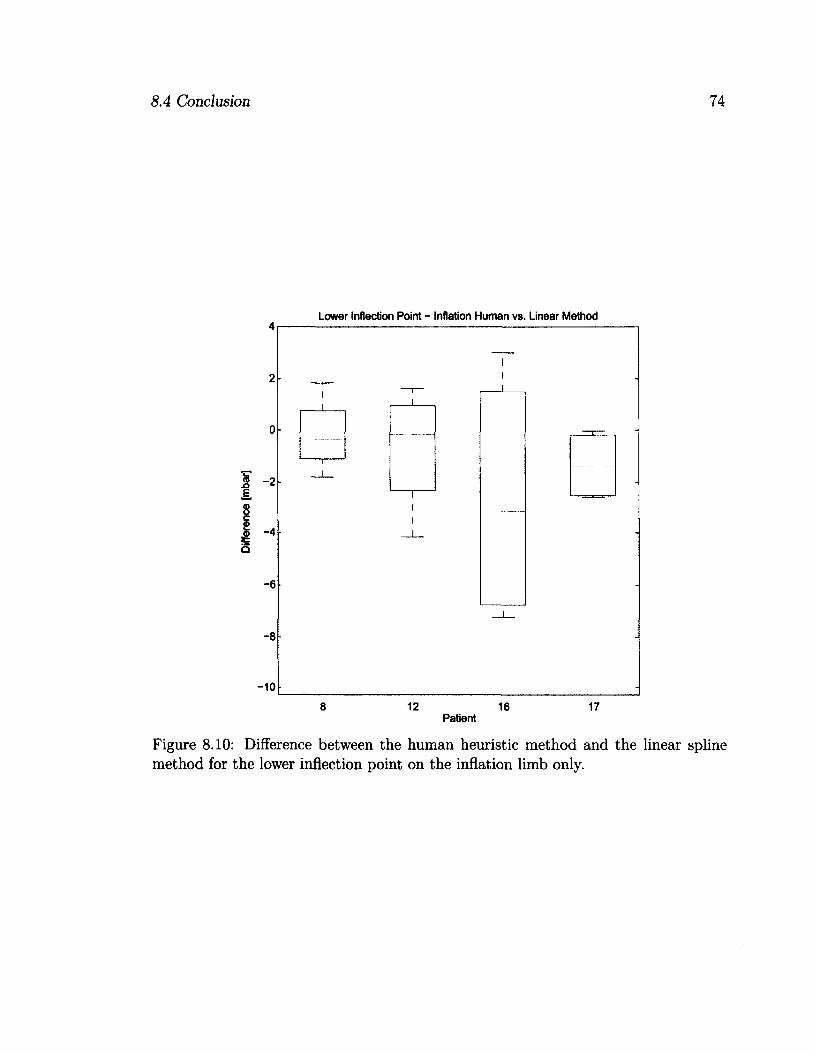
8.4 Conclusion 74
Lower Inflection Point - Inflation Human vs. Linear Method
12 16 Patient
Figure 8.10: Difference between the human heuristic method and the linear spline method for the lower inflection point on the inflation limb only.
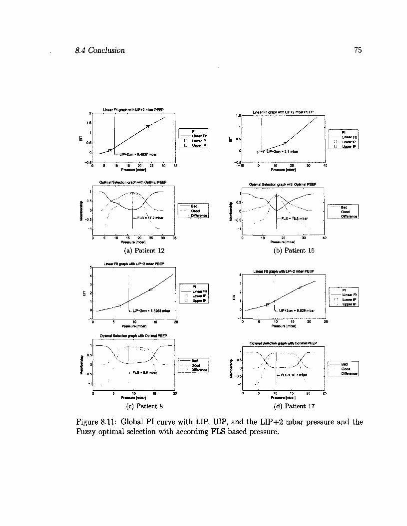
8.4 Conclusion 75
Linear Fit graph with LIP+2 mbar PEEP
Pi Linear Fit Lower IP
• Upper IP
LIP+2cm * 9.4837 mbar
10 15 20 25 30 Pressure [mbarj
Linear Fit graph with LIP+2 mbar PEEP
PI Linear Fit Lower IP
J Upper IP LIP+2cm • 2.1 mbar
10 20 Pressure [mbar]
Optimal Selection graph with Optimal PEEP
V -T X"
\ \ /
•
\ / «- FLS * 172 mbar
' \
Optima! Selection graph with Optimal PEEP
- Bad Good Difference
5 10 15 20 25 30 Pressure [mbar]
(a) Patient 12
Lineer Fit graph with LIP+2 mbar PEEP
PI Linear Fit Lower IP
• Upper IP
LiP+2cm * 8.5283 mbar
5 10 15 Pressure (mbar)
Optimal Selection graph with Optimal PEEP
X . „— •
\ ' 'V
«- FLS - 8.8 mbar(
-Bad Good Difference
5 10 15 Pressure (mbar)
(c) Patient 8
1
. 0.5
0 -0.5
-1
//
^ \
/ FLS « mbar
10 20 30 Pressure [mbar)
(b) Patient 16
Linear Fit graph with LIP+2 mbar PEEP
Optimal Selection graph with Optimal PEEP
Pressure (mbar)
(d) Patient 17
Bad Good Difference
Pi Linear FH Lower IP Upper IP
LIP+2cm * 9.828 mber
Pressure [mbar]
FLS = 10.3 mW
Figure 8.11: Global PI curve with LIP, UIP, and the LIP+2 mbar pressure and the Fuzzy optimal selection with according FLS based pressure.
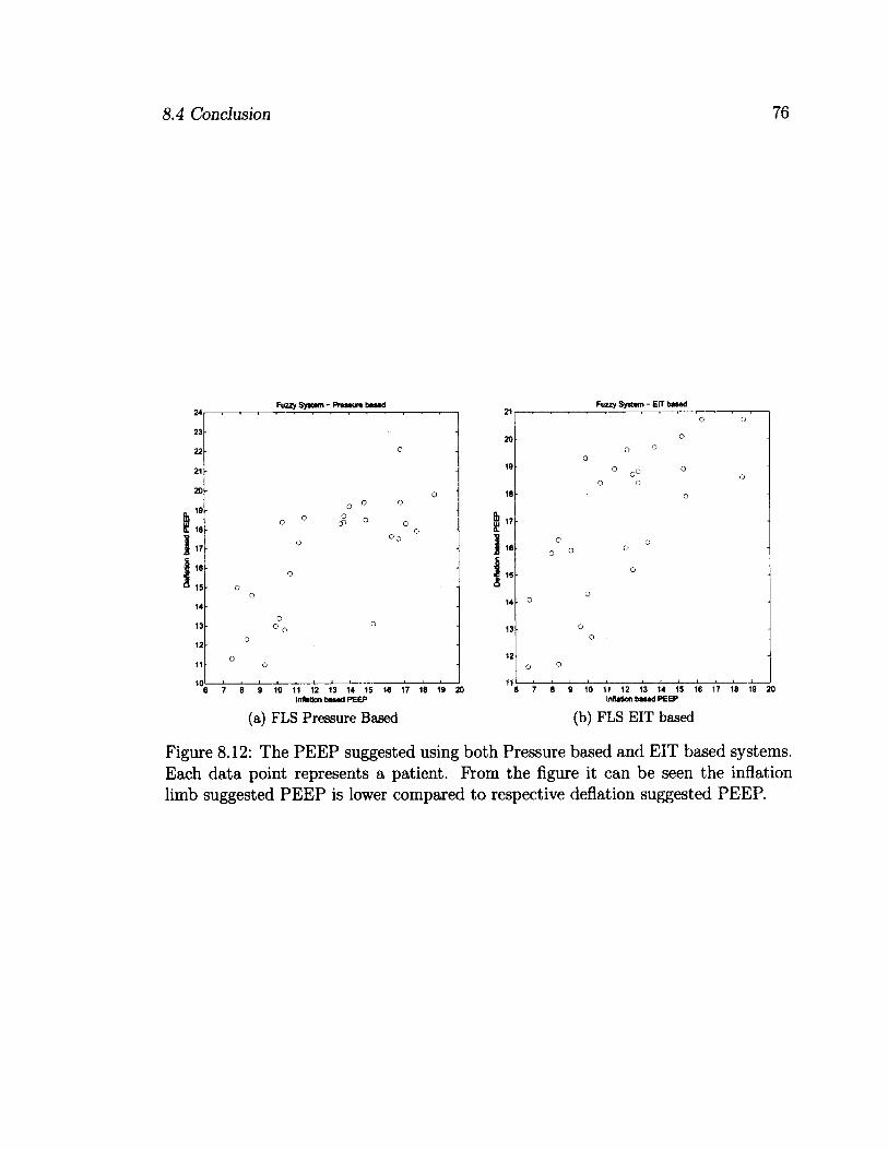
8.4 Conclusion 76
Fuzzy System - Pressure based
o
o o
0 o
0
o
o 3 °
o
o o
0
o
0
o
0 ° o o
o
o o
>
7 6 9 10 11 12 13 14 15 16 17 16 19 20 inflation based PEEP
(a) FLS Pressure Based
Fuzzy System - EIT based
0 o
o o o o
o o
o
0
o
o
o
o
o 0 o
o
o
0
. 0 0
o o
0 o
7 8 9 10 11 12 13 14 15 16 17 18 19 20 Inflation based PEEP
(b) FLS EIT based
Figure 8.12: The PEEP suggested using both Pressure based and EIT based systems. Each data point represents a patient. From the figure it can be seen the inflation limb suggested PEEP is lower compared to respective deflation suggested PEEP.

Chapter 9
Summary and Future Work
This work takes a novel step toward development of tools for automated PEEP selec
tion for mechanical ventilation systems. Using a quasi-static pressure based recruit
ment maneuver optimal PEEP was located to reduce lung injury conditions while
maximizing typical working lung tissue. Contributions to this task were locating re
gional Inflection Points (IP) to reduce collapsed and overdistended lung tissue known
to be factors of Ventilator Induce Lung Injury (VILI). Refer to Chapter 6 for a de
tailed study on locating IP. Additionally, using the lower and upper inflection points
(LIP and UIP) a Singleton Type-1 Fuzzy Logic System (FLS) was created to classify
lung regions as collapsed, normal, or overdistended. With the classifications a PEEP
was located. Details on the algorithm design can be seen in Chapter 7.
Evaluations were performed by comparing the recommended PEEP from this the
sis to the recommended value in the study conducted by [Takeuchi et al., 2002]. De
tails of the comparison can be seen in Chapter 8.3.
This work investigates the use of regional IP along with the tool used to locate
them, the linear spline technique [Grychtol et al., 2009]. It also investigates the use
of Fuzzy Logic in converting quantitative values and expert knowledge of mechanical
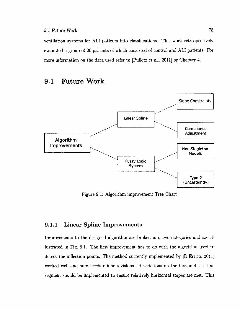
9.1 Future Work 78
ventilation systems for ALI patients into classifications. This work retrospectively
evaluated a group of 26 patients of which consisted of control and ALI patients. For
more information on the data used refer to [Pulletz et al., 2011] or Chapter 4.
9.1 Future Work
Non-Singleton Models
Slope Constraints
Type-2 (Uncertaintly)
Fuzzy Logic System
Linear Spline
Compliance Adjustment
Algorithm Improvements
Figure 9.1: Algorithm improvement Tree Chart
9.1.1 Linear Spline Improvements
Improvements to the designed algorithm are broken into two categories and are il
lustrated in Fig. 9.1. The first improvement has to do with the algorithm used to
detect the inflection points. The method currently implemented by [D'Errico, 2011]
worked well and only needs minor revisions. Restrictions on the first and last line
segment should be implemented to ensure relatively horizontal slopes are met. This
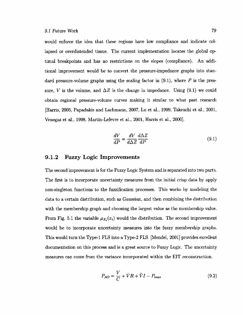
9.1 Future Work 79
would enforce the idea that these regions have low compliance and indicate col
lapsed or overdistended tissue. The current implementation locates the global op
timal breakpoints and has no restrictions on the slopes (compliance). An addi
tional improvement would be to convert the pressure-impedance graphs into stan
dard pressure-volume graphs using the scaling factor in (9.1), where P is the pres
sure, V is the volume, and AZ is the change in impedance. Using (9.1) we could
obtain regional pressure-volume curves making it similar to what past research
[Harris, 2005, Papadakis and Lachmann, 2007, Lu et al., 1999, Takeuchi et al., 2001,
Venegas et al., 1998, Martin-Lefevre et al., 2001, Harris et al., 2000].
dV _ dV dAZ dP ~ dAZ dP ^ }
9.1.2 Fuzzy Logic Improvements
The second improvement is for the Fuzzy Logic System and is separated into two parts.
The first is to incorporate uncertainty measures from the initial crisp data by apply
non-singleton functions to the fuzzification processes. This works by modeling the
data to a certain distribution, such as Gaussian, and then combining the distribution
with the membership graph and choosing the largest value as the membership value.
From Fig. 5.1 the variable would the distribution. The second improvement
would be to incorporate uncertainty measures into the fuzzy membership graphs.
This would turn the Type-1 FLS into a Type-2 FLS. [Mendel, 2001] provides excellent
documentation on this process and is a great source to Fuzzy Logic. The uncertainty
measures can come from the variance incorporated within the EIT reconstruction.
PAO — -Q + VR + VI — PmUs (9.2)
9.1 Future Work 80
A more novel improvement would be to tackle the assumption that the airway
pressure which is used with in the pressure-impedance calculations are the same
throughout the entire thorax [Costa et al., 2009].
In [Harris, 2005] the equation for airway pressure is used to model the changes in
pressure of the respiratory system. We can see this equation in (9.2) where V is the
volume, Cis the respiratory compliance, V is the volume flow, R is the respiratory
resistance, V is the volume acceleration, I is the respiratory impedance, and Pmus is
the pressure needed for respiratory muscle movement. All the variables listed assume
equal lung expansion as can be seen from the globular nature.
For quasi-static and static recruitment maneuvers all factors other than V and C
are ignored or negligible. The reason behind this is discussed in Chapter 2. Using
the regional information of EIT, the compliance conversion equation in (9.1), and
the measured volume provided by the mechanical ventilation system we can calculate
the regional compliance. Using the regional compliance and measured volume we
can calculate regional pressure values which can then by used for regional pressure-
impedance curves.
9.1.3 Future Testing
With the lack of a golden standard in the data this study was only able to compute
an optimal PEEP with no ground truth. With this being said a detailed study
should be conducted in which patients are monitored after apply this algorithms
suggested PEEP. From here we can record the survival rates along with the weaning
time. Comparing this set of patients to a control a sense of long term results can be
obtained. In terms of short term results CT scans can be taken and segmented into
overdistended and collapsed regions, from here comparison between the algorithm
in this thesis and the results from the CT scans can be compared. Finally arterial

9.1 Future Work 81
oxygen partial pressure, lung inflammation, and mRNA expressions can be taken at
the suggested PEEP and compared to other recommendations.
Overall this thesis sets out to develop an automated system to analyse EIT images
for the use of optimal PEEP selection. Its major contribution are: a) the testing of the
linear spline method for the detection of inflection points within pressure-impedance
curves, and b) the development of a fuzzy logic classification system. It is hoped that
the contributions in this thesis will inspire future work for the improvement of patient
care.

Appendix A
MATLAB Code
All code in this section was written and designed by [D'Errico, 2011]. With his
permission it was included in this thesis as it no longer appears online.
A.l Linear Spline
f u n c t i o n s p l = p l i n f i t ( x , y , n u m s e g , m i n l e n , d i s p i m g )
% c o m p u t e s a p i e c e w i s e l i n e a r l e a s t s q u a r e s s p l i n e w i t h o p t i m i z e d
% i n t e r n a l k n o t p l a c e m e n t . U s e s a p a r t i t i o n e d l e a s t s q u a r e s
% f o r t h e p a r a m e t e r e s t i m a t i o n .
%
% N o t e : t h e s p l i n e f i t w i l l b e i n a p i e c e w i s e H e r m i t e f o r m .
% a s I r e t u r n i t , t h e f i r s t c o l u m n o f s p l w i l l b e t h e l i s t
% o f b r e a k p o i n t s o f t h e s p l i n e , a n d t h e s e c o n d c o l u m n w i l l
% b e t h e v a l u e s o f t h e f u n c t i o n a t t h o s e p o i n t s .
%
% I t i s l e f t a s a n e x e r c i s e f o r t h e s t u d e n t t o f i g u r e o u t h o w t o
% e v a l u a t e t h e e s t i m a t e d f u n c t i o n a t a n y p o i n t x .
% c h e c k t o s e e i f t h i s c a l l i s r e a l l y a c a l l t o m y h i d d e n
% o b j e c t i v e f u n c t i o n .
i f i s s t r u c t ( y )
s p l = p l i n o b j ( x , y ) ;
r e t u r n
e n d
% m a k e s u r e x & y a r e c o l u m n v e c t o r s f o r c o n v e n i e n c e
% a l s o , s o r t t h e m f o r l a t e r c o n v e n i e n c e i n p l o t t i n g
82

A.l Linear Spline
[ x , t a g s ] = s o r t ( x ( : ) ) ;
y - y ( : ) ; y = y ( t a g s ) ;
i f ( n a r g i n < 4 ) | i s e m p t y ( m i n l e n )
m i n l e n = 0 ;
e n d
i f ( n a r g i n < 4 ) | i s e m p t y ( n u m s e g )
n u m s e g = 2 ;
e l s e i f n u m s e g < 2
e r r o r ' S o r r y , b u t I w a s l a z y , a n d I i n s i s t o n a t l e a s t 2 s e g m e n t s
e n d
% g e t s t a r t i n g v a l u e s f o r t h e k n o t s
k n o t O = l i n s p a c e ( m i n ( x ) , m a x ( x ) , n u m s e g + 1 ) ' ;
i f ( k n o t O ( 2 ) - k n o t O ( 1 ) ) C m i n l e n
e r r o r ' m i n l e n i s t o o l a r g e f o r t h a t m a n y k n o t s . '
e n d
% w e a r e g o i n g t o o p t i m i z e o n l y o v e r t h e i n t e r i o r k n o t s
k n o t O ( [ l , e n d ] ) = [ ] ;
n u m p a r a m = n u m s e g — 1 ;
% t h i s s t r u c t u r e w i l l c o n t a i n a l l w e n e e d i n t h e o b j e c t i v e f u n c t i o n
% I t s s i m p l e r t h i s w a y t h a n p a s s i n g i n m u l t i p l e e x t r a a r g u m e n t s .
p a s s i n . x = x ;
p a s s i n . y = y ;
p a s s i n . f i r s t = m i n ( x ) ;
p a s s i n . l a s t = m a x ( x ) ;
p a s s i n . n u m s e g = n u m s e g ;
% c r e a t e t h e i n e q u a l i t y c o n s t r a i n t a r r a y f o r f m i n c o n
A = z e r o s ( n u m p a r a m + 1 , n u m p a r a m ) ;
B = z e r o s ( n u m p a r a m + 1 , 1 ) ;
A ( l , 1 ) = — 1 ;
B ( 1 ) = m i n ( x ) + m i n l e n ;
f o r i = 2 : n u m p a r a m
A ( i , i + [ - l 0 ] ) = [ 1 - 1 ] ;
B ( i ) = m i n l e n ;
e n d
A ( n u m p a r a m + 1 , n u m p a r a m ) = 1 ;
B ( n u m p a r a m + 1 , 1 ) = m a x ( x ) — m i n l e n ;
% s e t a n y o p t i o n s h e r e
o p t i o n s = o p t i m s e t ( ' f m i n c o n ' ) ;
o p t i o n s = o p t i m s e t ( o p t i o n s , ' d i s p l a y ' , 1 o f f ' ) ;
o p t i o n s = o p t i m s e t ( o p t i o n s , ' l a r g e s c a l e ' , ' o n ' ) ;
o p t i o n s = o p t i m s e t ( o p t i o n s , ' A l g o r i t h m ' , ' a c t i v e — s e t ' ) ;
k n o t s = f m i n c o n ( ' p l i n f i t ' , k n o t O , A , B , [ ] , [ ] , [ ] , [ ] , [ ] , o p t i o n s , p a s s i n ) ;

A.l Linear Spline 84
% t a k e t h e i n t e r i o r k n o t s f o u n d f r o m f m i n c o n a n d g e t t h e
% f i n a l s p l i n e f r o m p l i n o b j
[ j u n k , s p l , p r e d ] = p l i n o b j ( k n o t s , p a s s i n ) ;
% p l o t t h e r e s u l t s
i f ( d i s p i m g )
p l o t ( x , y , ' r . 1 )
h o l d o n
p l o t ( s p l ( : , 1 ) , s p l ( : , 2 ) , ' b - ' )
p l o t ( s p l ( 2 , 1 ) , s p l ( 2 , 2 ) , ' g s ' ) ;
p l o t ( s p l ( 3 , 1 ) , s p l ( 3 , 2 ) , • g s ' ) ;
h o l d o f f
e n d
% A l l d o n e . T h a t w a s n ' t s o h a r d a f t e r a l l .
% e n d o f m a i n l i n e p l i n f i t f u n c t i o n , b e g i n h i d d e n o b j e c t i v e f u n c t i o n
f u n c t i o n [ o b j , s p l , p r e d ] = p l i n o b j ( i n t e r i o r - k n o t s , p a s s i n )
% e s t i m a t e p i e c e w i s e l i n e a r l e a s t s q u a r e s s p l i n e g i v e n a f i x e d
% s e t o f k n o t s .
k n o t s = s o r t ( [ p a s s i n . f i r s t ; i n t e r i o r _ k n o t s ; p a s s i n . l a s t ] ) ;
d e l t a = d i f f ( k n o t s ) ;
% u s e b i n d e x t o b i n t h e d a t a p o i n t s
i n t e r v a l = b i n d e x ( p a s s i n . x , k n o t s , 1 ) ;
t = ( p a s s i n . x — k n o t s ( i n t e r v a l ) ) . / d e l t a ( i n t e r v a l ) ;
% b u i l d l i n e a r l e a s t s q u a r e p r o b l e m s p a r s e l y f o r f u n
n = l e n g t h ( p a s s i n . x ) ;
d e s m a t = s p a r s e ( ( 1 : n ) 1 , i n t e r v a l , 1 — t , n , p a s s i n . n u m s e g + 1 ) ;
d e s m a t = d e s m a t + s p a r s e ( ( 1 : n ) ' , i n t e r v a l + 1 , t , n , p a s s i n . n u m s e g + 1 ) ;
% s o l v e
c o e f = f u l l ( d e s m a t \ p a s s i n . y ) ;
% c o m p u t e p r e d i c t i o n s
p r e d = f u l l ( d e s m a t * c o e f ) ;
% r e t u r n t h e o b j e c t i v e f u n c t i o n a s a s u m o f s q u a r e s o f e r r o r s .
o b j = s u m ( ( p a s s i n . y — p r e d ) . " 2 ) ;
% o n l y r e t u r n t h e s p l i n e i t s e l f i f t w o o u t p u t a r g u m e n t s
i f n a r g o u t > l
s p l = [ k n o t s , c o e f ] ;
e n d
% e n d m - f i l e

A.J Linear Spline
A. 1.1 Bin function needed for Spline
f u n c t i o n i n d = b i n d e x ( x t e s t , b i n l b , c l i p - f l a g , m e t h o d - f l a g )
% b i n d e x : i d e n t i f i e s w h i c h b i n t e s t p o i n t s f a l l i n t o
% u s a g e : i n d = b i n d e x ( x t e s t , b i n l b , c l i p . f l a g , m e t h o d - f l a g )
%
% a r g u m e n t s :
% x t e s t — s e t o f o n e o r m o r e p o i n t s t o a s s i g n i n t o a l i s t o f b i n s
%
% b i n l b — l i s t o f l o w e r b o u n d s o f b i n s i n i n c r e a s i n g o r d e r .
% T h e l a s t e l e m e n t i n t h i s v e c t o r i s t h e u p p e r b o u n d
% o f t h e l a s t b i n .
% N o t e : t h i s v e c t o r m u s t b e s o r t e d i n i n c r e a s i n g o r d e r .
% I d o n o t t e s t f o r t h i s p r o p e r t y .
%
% c l i p _ f l a g - O P T I O N A L s c a l a r f l a g - b i n n i n g h a s o n e p r o b l e m -
% i . e . , w h a t d o y o u d o w i t h t e s t p o i n t s b e l o w t h e f i r s t
% b i n ' s l o w e r b o u n d o r a b o v e t h e l a s t b i n ?
%
% c l i p - f l a g s p e c i f i e s w h e t h e r t e s t p o i n t s b e l o w t h e
% l o w e s t b i n a r e a s s i g n e d b i n 0 o r b i n 1 . l i k e w i s e
% p o i n t s a b o v e t h e h i g h e s t b i n m u s t b e d e a l t w i t h t o o .
%
% n o m i n a l l y , a t e s t p o i n t i s i n t h e i ' t h b i n i f
%
% b i n l b ( i ) < = x t e s t ( j ) < b i n l b ( i + l )
%
% i f a p o i n t f a l l s b e l o w t h e l o w e s t b i n , t h e n
% t h i s d e f i n i t i o n s u g g e s t s i t f a l l s i n b i n 0 .
% a b o v e b i n l b ( e n d ) , t h i s d e f i n i t i o n p u t s a p o i n t
% i n b i n n u m b e r n b i n .
%
% c l i p . f l a g = = 0 — > ( t h e d e f a u l t ) l e a v e p o i n t s o u t s i d e
% t h e b i n s , a n d r e t u r n 0 o r n b i n s
% c l i p - f l a g = = l — > p u t p o i n t s b e l o w i n b i n # 1 , a n d
% p o i n t s a b o v e i n b i n # n b i n s - 1
%
% m e t h o d - f l a g — O P T I O N A L s c a l a r f l a g — a l l o w s t h e u s e r t o
% c h o o s e w h i c h b i n n i n g a l g o r i t h m t o u s e . I f n o t s p e c i f i e d ,
% t h e n t h e m e t h o d i s c h o s e n v i a a s i m p l e h e u r i s t i c .
%
% m e t h o d . f l a g = = l — > l o o p o v e r t e s t p o i n t s
% m e t h o d - f l a g = = 2 — > l o o p o v e r b i n s
% m e t h o d _ f l a g = = 3 — > s o r t
% m e t h o d - f l a g = = 4 — > h a s h t a b l e
%
% i n d — a r r a y o f i n d i c i e s o f t h e b i n ( s ) i n t o w h i c h x t e s t f e l l
% a u t h o r : J o h n R . D ' E r r i c o
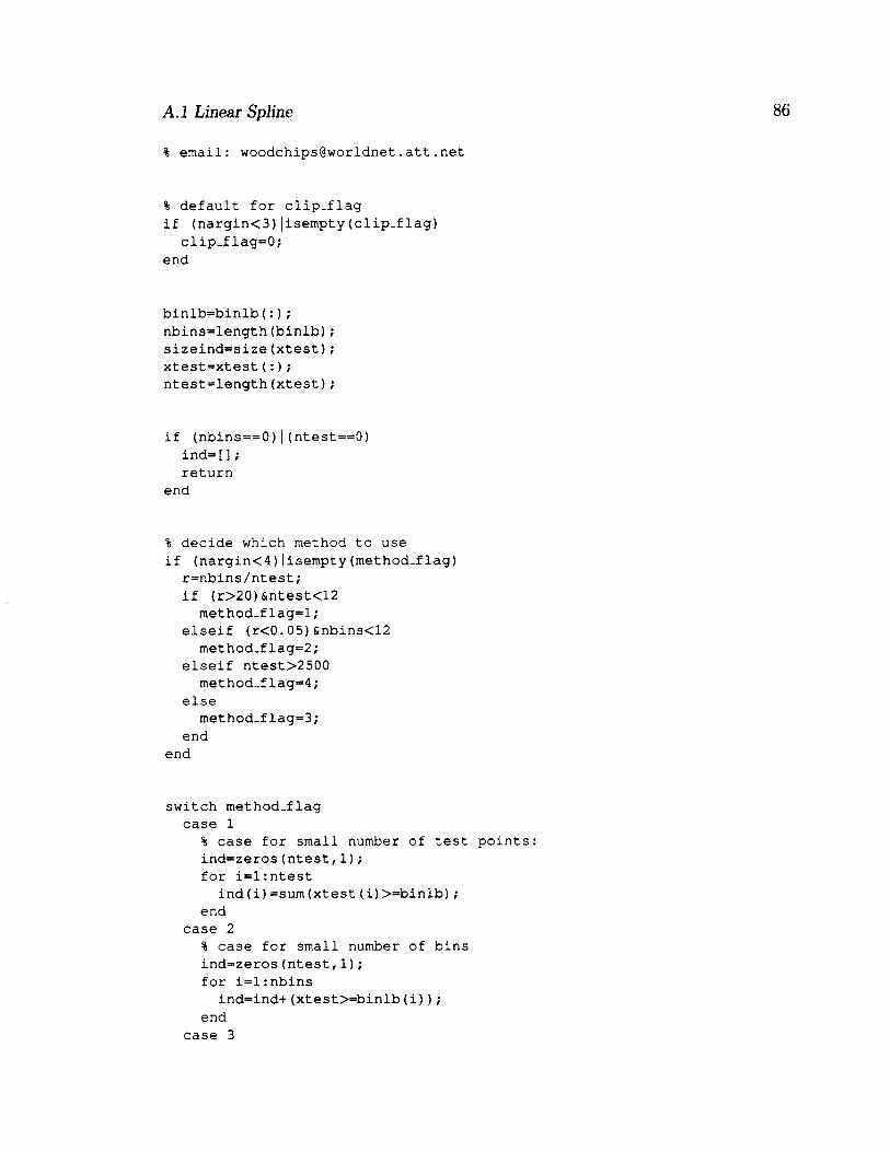
A.J Linear Spline 86
% e m a i l : w o o d c h i p s @ w o r l d n e t . a t t . n e t
% d e f a u l t f o r c l i p . f l a g
i f ( n a r g i n < 3 ) | i s e m p t y ( c l i p . f l a g )
c l i p - f l a g = 0 ;
e n d
b i n l b = b i n l b ( : ) ;
n b i n s = l e n g t h ( b i n l b ) ;
s i z e i n d = s i z e ( x t e s t ) ;
x t e s t = x t e s t ( : ) ;
n t e s t = l e n g t h ( x t e s t ) ;
i f ( n b i n s = = 0 ) | ( n t e s t = = 0 )
i n d = [ ] ;
r e t u r n
e n d
% d e c i d e w h i c h m e t h o d t o u s e
i f ( n a r g i n < 4 ) | i s e m p t y ( m e t h o d - f l a g )
r = n b i n s / n t e s t ;
i f ( r > 2 0 ) & n t e s t < 1 2
m e t h o d . f l a g = l ;
e l s e i f ( r < 0 . 0 5 ) & n b i n s < 1 2
m e t h o d . f l a g = 2 ;
e l s e i f n t e s t > 2 5 0 0
m e t h o d . f l a g = 4 ;
e l s e
m e t h o d . f l a g = 3 ;
e n d
e n d
s w i t c h m e t h o d - f l a g
c a s e 1
% c a s e f o r s m a l l n u m b e r o f t e s t p o i n t s :
i n d = z e r o s ( n t e s t , 1 ) ;
f o r i = l : n t e s t
i n d ( i ) = s u m ( x t e s t ( i ) > = b i n l b ) ;
e n d
c a s e 2
% c a s e f o r s m a l l n u m b e r o f b i n s
i n d = z e r o s ( n t e s t , 1 ) ;
f o r i = l : n b i n s
i n d = i n d + ( x t e s t > = b i n l b ( i ) ) ;
e n d
c a s e 3

A.l Linear Spline
% s o r t s o l u t i o n
[ x x i , j ] = s o r t ( x t e s t ) ;
[ d u m , i ] = s o r t ( [ b i n l b ; x x i ] ) ;
i n d ( i ) = 1 : l e n g t h ( i ) ;
i n d = ( i n d ( n b i n s + ( 1 : n t e s t ) ) — ( 1 r n t e s t ) ) ' ;
i n d ( j ) = i n d ;
c a s e 4
% h a s h t a b l e s o l u t i o n
i n d = z e r o s ( n t e s t , 1 ) ;
m v = i n d ;
b l = b i n l b ( 1 ) ;
b n = b i n l b ( e n d ) ;
% s i z e o f h a s h t a b l e i s d e p e n d e n t o n t h e n u m b e r o f n o d e s ,
% a n d h o w c l o s e t o u n i f o r m t h e s p a c i n g i s .
a v e . s p a c e = ( b n - b l ) / ( n b i n s - 1 ) ;
m i n _ s p a c e = m i n ( d i f f ( b i n l b ) ) ;
m a x _ h a s h = 1 5 0 0 ;
n h a s h = r o u n d ( m i n ( m a x . h a s h , ( n b i n s — 1 ) * a v e . s p a c e / m i n _ s p a c e ) ) ;
h a s h _ x = b l + ( b n — b l ) * ( ( 1 : n h a s h ) . 5 ) / ( n h a s h ) ;
h a s h _ t a b l e = [ b i n d e x ( h a s h _ x , b i n l b ) ; n b i n s - 1 ] ;
i n d ( x t e s t > = b n ) = n b i n s ;
k = f i n d ( ( x t e s t > = b l ) & ( x t e s t < b n ) ) ;
% e s t i m a t e b i n a s s i g n m e n t
i n d ( k ) = h a s h _ t a b l e ( 1 + f l o o r ( ( x t e s t ( k ) - b l ) / ( ( b n — b l ) / n h a s h ) ) )
% l o o k f o r a n y p o i n t s t h a t a r e b e l o w t h e i r b i n a s s i g n m e n t
k d e c = k ( x t e s t ( k ) < b i n l b ( i n d ( k ) ) ) ;
w h i l e " i s e m p t y ( k d e c )
i n d ( k d e c ) = i n d ( k d e c ) — 1 ;
j = ( x t e s t ( k d e c ) > = b i n l b ( i n d ( k d e c ) ) ) ;
i f a n y ( j )
k d e c ( j ) = [ ] ;
e n d
e n d
% l o o k f o r a n y p o i n t s t h a t a r e a b o v e t h e i r b i n a s s i g n m e n t
k i n c = k ( x t e s t ( k ) > = b i n l b ( i n d ( k ) + 1 ) ) ;
w h i l e " i s e m p t y ( k i n c )
i n d ( k i n c ) = i n d ( k i n c ) + 1 ;
j = ( x t e s t ( k i n c ) < b i n l b ( i n d ( k i n c ) + 1 ) ) ;
i f a n y ( j )
k i n c ( j ) = [ ] ;
e n d
e n d
e n d

A.l Linear Spline 88
% b e n i c e a n d r e t u r n i n d i c e s a s t h e s a m e s h a p e a s x t e s t .
i n d = r e s h a p e ( i n d , s i z e i n d ) ;
% d o w e r e t u r n a b i n i n d e x b e l o w 1 o r a b o v e n b i n - 1 ?
i f c l i p _ f l a g
i n d = m a x ( l , m i n ( n b i n s — 1 , i n d ) ) ;
e n d
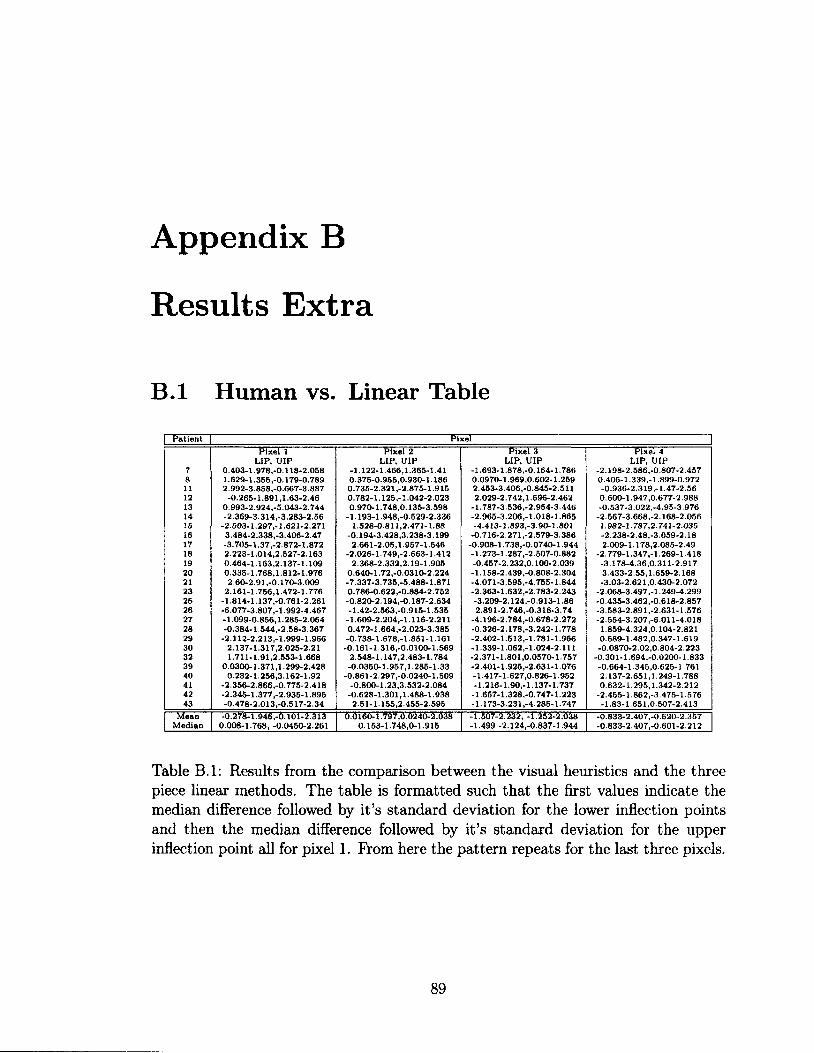
Appendix B
Results Extra
B.l Human vs. Linear Table
Patient Pixel
Pixel 1 Pixel 2 Pixel 3 Pixel 4 LIP, UIP LIP, UIP LIP, UIP LIP, UIP
7 0.403-1.978,-0.118-2.058 -1.122-1.466,1.365-1.41 -1.693-1.878,-0.164-1.786 -2.198-2.586,-0.807-2.457 8 1.629-1.355,-0.179-0.789 0.375-0.955,0.930-1.186 0.0970-1.969,0.602-1.259 0.405-1.339,-1 899-0.972 11 2.992-3.858,-0.667-3.887 0.735-2.321,-2.875-1.915 2.453-3.406,-0.845-2.511 -0.936-2.319,-1-47-2.56 12 -0.265-1.891,1.63-2.46 0.782-1.125,-1.042-2.023 2.029-2.742,1.696-2.462 0.600-1.947,0.677-2.988 13 0.993-2.924,-5.043-2.744 0.970-1.748,0.135-3.598 -1.787-3.536,-2.954-3.446 -0.537-3.022,-4.95-3.976 14 -2.369-3.314,-3.283-2.56 -1.193-1.948,-0.529-2.336 -2.965-3.206,-1.018-1.865 -2.567-3.668,-2.168-2.056 25 -2.503-1.297,-1.621-2.271 1.528-0.811,2.471-1.88 -4.413-1.893,-3.90-1.801 1.982-1.787,2.741-2.035 16 3.484-2.338,-3.406-2.47 -0.194-3.428,3.238-3.199 -0.716-2.271,-2.579-3.386 -2.238-2.48,-3.059-2.18 17 -3.705-1.37,-2.872-1.872 2.661-2.05,1.957-1.546 -0.908-1.738,-0.0740-1.944 2.009-1.178,2.085-2.49 18 2.223-1.014,2.527-2.163 -2.026-1.749,-2.663-1.412 -1.273-1.287,-2.507-0.882 -2.779-1.347,-1.269-1.418 19 0.464-1.163,2.137-1.109 2.368-2.332,2.19-1.905 -0.457-2.232,0.100-2.039 -3.178-4.36,0.311-2.917 20 0.335-1.768,1.812-1.976 0.640-1.72,-0.0310-2.224 -1.158-2.439,-0.808-2.304 3.433-2.55,1.659-2.168 21 2.60-2.91,-0.170-3.009 -7.337-3.735,-5.488-1.871 -4.071-3.595,-4.755-1.844 -3.03-2.621,0.430-2.072 23 2.161-1.756,1.472-1.776 0.786-0.622,-0.884-2.752 -2.363-1.632,-2.783-2.243 -2.068-3.497,-1.249-4.299 25 -1.814-1.137,-0.761-2.261 -0.820-2.194,-0.187-2.634 -3.209-2.124,-0.913-1.86 -0.435-3.462,-0.618-2.857 26 -6.077-3.807,-1.992-4.467 -1.42-2.563,-0.915-1.535 2.891-2.746,-0.316-3.74 -3.583-2.891,-2.631-1.576 27 -1.099-0.856,1.285-2.064 -1.609-2.204,-1.116-2.211 -4.196-2.784,-0.678-2.272 -2.554-3.207,-6.011-4.018 28 -0.384-1.544,-2.58-3.367 0.472-1.664,-2.023-3.385 -0.326-2.178,-3.242-1.778 1.859-4.324,0.104-2.821 29 -2.112-2.213,-1.999-1.966 -0.738-1.678,-1.851-1.161 -2.402-1.513,-1.781-1.966 0.589-1.482,0.347-1.619 30 2.137-1.317,2.025-2.21 -0.161-1.316,-0.0100-1.569 -1.339-1.062,-1.024-2.111 -0.0870-2.02,0.804-2.223 32 1.711-1.91,2.553-1.668 2.548-1.147,2.483-1.784 -2.371-1.801,0.0570-1.757 -0.301-1.694,-0.0200-1.833 39 0.0300-1.371,1.299-2.428 -0.0350-1.957,1.285-1.33 -2.401-1.925,-2.631-1.076 -0.664-1.345,0.625-1.761 40 0.232-1.256,3.162-1.92 -0.861-2.297,-0.0240-1.509 -1.417-1.627,0.826-1.952 2.137-2.651,1.249-1.788 41 -2.356-2.866,-0.775-2.418 -0.800-1.23,3.532-2.084 -1.216-1.90,-1.137-1.737 0.632-1.295,1.342-2.212 42 -2.345-1.377,-2.935-1.895 -0.628-1.301,1.488-1.938 -1.657-1.328,-0.747-1.223 -2.455-1.862,-3.475-1.576 43 -0.478-2.013,-0.517-2.34 2.51-1.155,2.455-2.595 -1.173-3.231,-4.285-1.747 -1.83-1.651,0.507-2.413
Mean -0.278-1.946,-0.101-2.313 0.0160-1.797,0.0240-2.038 -1.507-2.232, -1.252-2.038 -0.833-2.407,-0.620-2.357 Median 0.008-1.768, -0.0450-2.261 0.153-1.748,0-1.915 -1.499 -2.124,-0.837-1.944 -0.833-2.407,-0.601-2.212
Table B.l: Results from the comparison between the visual heuristics and the three piece linear methods. The table is formatted such that the first values indicate the median difference followed by it's standard deviation for the lower inflection points and then the median difference followed by it's standard deviation for the upper inflection point all for pixel 1. Prom here the pattern repeats for the last three pixels.
89
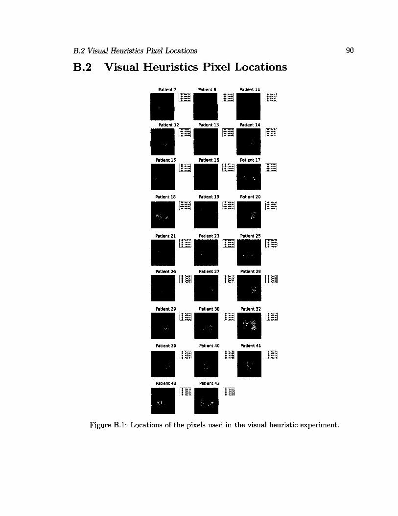
B.2 Visual Heuristics Pixel Locations
B.2 Visual Heuristics Pixel Locations
Patient 7 Patient 8 Patient 11
Patient 12 Patient 13 Patient 14
Patient 17 Patient 15 Patient 16
Patient 18 Patient 19 Patient 20
Patient 21 Patient 23 Patient 25
Patient 26 Patient 27 Patient 28
Patient 29 Patient 30 Patient 32
Patient 39 Patient 40 Patient 41
Patient 42 Patient 43
Figure B.l: Locations of the pixels used in the visual heuristic experiment.

References
[Adler et al., 2012] Adler, A., Amato, M., Arnold, J., Bayford, R., Bodenstein, M.,
Bohm, S., Brown, B., Frerichs, I., Stenqvist, O., Weiler, N., and Wolf, G. (2012).
Whither lung EIT: where are we, where do we want to go, and what do we need
to get there? Submitted for publication to Journal of Applied Physiology.
[Adler et al., 1997] Adler, A., Amyot, R., Guardo, R., Bates, J. H. T., and Berthi-
aume, Y. (1997). Monitoring changes in lung air and liquid volumes with electrical
impedance tomography. Journal of Applied Physiology, 83(5):1762-1767.
[Adler et al., 2009] Adler, A., Arnold, J. H., Bayford, R., Borsic, A., Brown, B.,
Dixon, R, Faes, T. J. C., Frerichs, I., Gagnon, H., Garber, Y., Grychtol, B., Hahn,
G., Lionheart, W. R. B., Malik, A., Patterson, R. P., Stocks, J., Tizzard, A.,
Weiler, N., and Wolf, G. K. (2009). GREIT: a unified approach to 2D linear EIT
reconstruction of lung images. Physiological Measurement, 30(6) :S35.
[Adler et al., 2011] Adler, A., Gaburro, R., and Lionheart, W. (2011). Handbook in
Mathematical Methods in Imaging. XVIII. Springer, 1 edition.
[Adler and Guardo, 1996a] Adler, A. and Guardo, R. (1996a). Electrical impedance
tomography: regularized imaging and contrast detection. Medical Imaging, IEEE
Transactions on, 15(2):170—179.
91

REFERENCES 92
[Adler and Guardo, 1996b] Adler, A. and Guardo, R. (1996b). Electrical impedance
tomography: Regularized imaging and contrast detection. IEEE Transaction on
Medical Imaging, 15(2):170-179.
[Adler et al., 1996] Adler, A., Guardo, R., and Berthiaume, Y. (1996). Impedance
imaging of lung ventilation: do we need to account for chest expansion? Biomedical
Engineering, IEEE Transactions on, 43(4):414-420.
[Adler and Lionheart, 2006] Adler, A. and Lionheart, W. R. B. (2006). Uses and
abuses of EIDORS: an extensible software base for EIT. Physiological Measurement,
27(5):S25.
[Albaiceta et al., 2004] Albaiceta, G. M., Taboada, F., Parra, D., Luyando, L. H.,
Calvo, J., Menendez, R., and Otero, J. (2004). Tomographic study of the inflection
points of the pressure-volume curve in acute lung injury. Am. J. Respir. Crit. Care
Med., 170(10):1066-1072.
[Allud and Martin, 1977] Allud, L. A. and Martin, M. H. (1977). Schlumberger: The
history of a technique. John Wiley and Sons, New York.
[Amato et al., 1995] Amato, M. B., Barbas, C. S., Medeiros, D. M., de P Schettino,
G., Filho, G. L., Kairalla, R. A., Deheinzelin, D., Morais, C., de O Fernandes, E.,
Takagaki, T. Y., and et al (1995). Beneficial effects of the "open lung approach"
with low distending pressures in acute respiratory distress syndrome. A prospec
tive randomized study on mechanical ventilation. Am J Respir Crit Care Med.,
152:1835-1846.
[Amato et al., 1998] Amato, M. B. P., Barbas, C. S. V., Medeiros, D. M., Maga-
ldi, R. B., Schettino, G. P., Lorenzi-Filho, G., Kairalla, R. A., Deheinzelin, D.,
Munoz, C., Oliveira, R., Takagaki, T. Y., and Carvalho, C. R. R. (1998). Effect

REFERENCES 93
of a protective-ventilation strategy on mortality in the acute respiratory distress
syndrome. New England Journal of Medicine, 338(6):347-354.
[Andersen, 2008] Andersen, M. H. (2008). Investigation of lung mechanics using CT
scan analysis, a mathematical model and the static pressure volume curve. Master's
thesis, Aalborg University.
[Aster et al., 2004] Aster, R. C., Borchers, B., and Thurber, C. (2004). Parameter
Estimation and Inverse Problems, chapter 2.2. Elsevier Academic Press.
[Bernard et al., 1994] Bernard, G., Artigas, A., Brigham, K., Carlet, J., Falke, K.,
Hudson, L., Lamy, M., Legall, J., Morris, A., and Spragg, R. (1994). The american-
european consensus conference on ARDS. definitions, mechanisms, relevant out
comes, and clinical trial coordination. Am. J. Respir. Crit. Care Med., 149(3):818-
824.
[Bigatello et al., 1999] Bigatello, William, H., and Antonio, P. (1999). Ventilatory
management of severe acute respiratory failure for Y2K. Anesthesiology, 91(6).
[Bindslev et al., 1980] Bindslev, L., Hedenstierna, G., Santesson, J., Norlander, O.,
and Gram, I. (1980). Airway closure during anaesthesia, and its prevention by
positive end expiratory pressure. Acta Anaesthesiologica Scandinavica, 24(3): 199-
205.
[Borcea, 2002] Borcea, L. (2002). Electrical impedance tomography. Inverse Prob
lems, 18(6):R99.
[Borges et al., 2006] Borges, J. B., Okamoto, V. N., Matos, G. F. J., Caramez, M.
P. R., Arantes, P. R., Barros, F., Souza, C. E., Victorino, J. A., Kacmarek, R. M.,
Barbas, C. S. V., Carvalho, C. R. R., and Amato, M. B. P. (2006). Reversibility

REFERENCES 94
of lung collapse and hypoxemia in early acute respiratory distress syndrome. Am.
J. Respir. Crit. Care Med., 174(3):268-278.
[Boyle, 2010] Boyle, A. J. S. (2010). The effect of shape deformation on two-
dimensional electrical impedance tomography. Master's thesis, Carleton University.
[Brunet et al., 1995] Brunet, F., Jeanbourquin, D., Monchi, M., Mira, J., Fierobe, L.,
Armaganidis, A., Renaud, B., Belghith, M., Nouira, S., and Dhainaut, J. (1995).
Should mechanical ventilation be optimized to blood gases, lung mechanics, or
thoracic CT scan? Am. J. Respir. Crit. Care Med., 152(2):524-530.
[Carlton et al., 1990] Carlton, D. R, Cummings, J. J., Scheerer, R. G., Poulain, F. R.,
and Bland, R. D. (1990). Lung overexpansion increases pulmonary microvascular
protein permeability in young lambs. Journal of Applied Physiology, 69(2):577-583.
[Colebatch et al., 1979] Colebatch, H. J., Ng, C. K., and Nikov, N. (1979). Use of an
exponential function for elastic recoil. Journal of Applied Physiology, 46(2) :387-
393.
[Costa et al., 2009] Costa, E., Borges, J., Melo, A., Suarez-Sipmann, F., Toufen, C.,
Bohm, S., and Amato, M. (2009). Bedside estimation of recruitable alveolar collapse
and hyperdistension by electrical impedance tomography. Intensive Care Medicine,
35:1132-1137.
[Coulombe et al., 2005] Coulombe, N., Gagnon, H., Marquis, F., Skrobik, Y., and
Guardo, R. (2005). A parametric model of the relationship between EIT and total
lung volume. Physiological Measurement, 26(4):401.
[Dambrosio et al., 1997] Dambrosio, M., Roupie, E., Mollet, J.-J., Anglade, M.-C.,
Vasile, N., Lemaire, F., and Brochard, L. (1997). Effects of positive end-expiratory

REFERENCES 95
pressure and different tidal volumes on alveolar recruitment and hyperinflation.
Anesthesiology, 87:495-503.
[de Abreu et al., 2003] de Abreu, M. G., Heintz, M., Heller, A., Szechenyi, R., Al-
brecht, D. M., and Koch, T. (2003). One-lung ventilation with high tidal volumes
and zero positive end-expiratory pressure is injurious in the isolated rabbit lung
model. Anesthesia and Analgesia, 96(l):220-228.
[D'Errico, 2011] D'Errico, J. (2011). MATLAB central - file exchange. http://www.
mathworks.com/matlabcentral/fileexchange/authors/679.
[Dreyfus and Saumon, 1998] Dreyfus, D. and Saumon, G. (1998). Ventilator-induced
lung injury, lessons from experimental studies. Am. J. Respir. Crit. Care Med,
S31-43.
[Dreyfuss and Saumon, 1993] Dreyfuss, D. and Saumon, G. (1993). Role of tital
volume, FRC, and end-inspiratory volume in the deveolopment of pulmonary edema
following mechanical ventilation. Am Rev Respir Dis, 148:1194-1203.
[EIDORS, 2011] EIDORS (2011). EIDORS: Electrical impedance tomography
and diffuse optical tomography reconstruction software. http://eidors3d.
sourceforge.net/.
[Faes et al., 2006] Faes, T. J. C., van Genderingen, H. R., and Noordegraaf, A. V.
(2006). Some reflections on the EIT conference (London, UK, 22-24 June 2005).
Physiological Measurement, 27(5).
[Frerichs et al., 2003] Frerichs, I., Dargaville, P., Dudykevych, T., and Rimensberger,
P. (2003). Electrical impedance tomography: a method for monitoring regional lung
aeration and tidal volume distribution? Intensive Care Medicine, 29.

REFERENCES 96
[Frerichs et al., 2002] Frerichs, I., Hinz, J., Herrmann, P., Weisser, G., Hahn, G.,
Dudykevych, T., Quintel, M., and Hellige, G. (2002). Detection of local lung air
content by electrical impedance tomography compared with electron beam CT.
Journal of Applied Physiology, 93(2):660-666.
[Fu et al., 1992] Fu, Z., Costello, M. L., Tsukimoto, K., Prediletto, R., Elliott, A. R.,
Mathieu-Costello, 0., and West, J. B. (1992). High lung volume increases stress
failure in pulmonary capillaries. Journal of Applied Physiology, 73(1): 123—133.
[Gattinoni et al., 1987] Gattinoni, L., Pesenti, A., Avalli, L., Rossi, F., and Bombino,
M. (1987). Pressure-volume curve of total respiratory system in acute respira
tory failure: Computed tomographic scan study. Am. J. Respir. Crit. Care Med.,
136(3):730-736.
[Gattinoni et al., 1984] Gattinoni, L., Pesenti, A., Caspani, M;.; Pelizzola, A.,
Mascheroni, D., Marcolin, R., Iapichino, G., Langer, M., Agostoni, A., Kolobow,
T., Melrose, D., and Damia, G. (1984). The role of total static lung compliance in
the management of severe ARDS unresponsive to conventional treatment. Intensive
Care Medicine, 10:121-126.
[Genderingen et al., 2004] Genderingen, H. R. V., Van Vught, A. J., and Jansen, J.
R. C. (2004). Regional lung volume during high-frequency oscillatory ventilation
by electrical impedance tomography. Critical Care Medicine, 32(3):787-794.
[Graham, 2007] Graham, B. M. (2007). Enhancements in Electrical Impedance To
mography (EIT) Image Reconstruction for 3D Lung Imaging. PhD thesis, Univer
sity of Ottawa.

REFERENCES 97
[Greenleaf et al., 2003] Greenleaf, A., Lassas, M., and Uhlmann, G. (2003).
Anisotropic conductivities that cannot be detected by EIT. Physiological Mea
surement, 24(2) :413.
[Grychtol et al., 2010] Grychtol, B., Wolf, G. K., Adler, A., and Arnold, J. H. (2010).
Towards lung EIT image segmentation: automatic classification of lung tissue state
from analysis of EIT monitored recruitment manoeuvres. Physiological Measure
ment, 31(8):S31.
[Grychtol et al., 2009] Grychtol, B., Wolf, G. K., and Arnold, J. H. (2009). Differ
ences in regional pulmonary pressure impedance curves before and after lung injury
assessed with a novel algorithm. Physiological Measurement, 30(6):S137.
[Hahn et al., 1996] Hahn, G., Frerichs, I., Kleyer, M., and Hellige, G. (1996). Local
mechanics of the lung tissue determined by functional EIT. Physiological Measure
ment, 17(4A):A159.
[Harris, 2005] Harris, R. S. (2005). Pressure-volume curves of the respiratory system.
Respiratory Care, 50(l):78-99.
[Harris et al., 2000] Harris, R. S., Hess, D. R., and Venegas, J. G. (2000). An ob
jective analysis of the pressure-volume curve in the acute respiratory distress syn
drome. Am. J. Respir. Crit. Care Med., 161(2):432-439.
[Hasan, 2010] Hasan, A. (2010). Understanding Mechanical Ventilation A Practical
Handbook. Springer-Verlab London Limited.
[Hickling, 1998] Hickling, K. G. (1998). The pressure-volume curve is greatly modified
by recruitment. A mathematical model of ARDS lungs. Am. J. Respir. Crit. Care
Med., 158(l):194-202.

REFERENCES 98
[Hinz et al., 2003a] Hinz, Hahn, Neumann, Sydow, Mohrenweiser, Hellige, and Bur-
chardi (2003a). End-expiratory lung impedance change enables bedside monitoring
of end-expiratory lung volume change. Intensive Care Medicine, 29:37-43.
[Hinz et al., 2006] Hinz, J., Moerer, O., Neumann, P., Dudykevych, T., Frerichs, I.,
Hellige, G., and Quintel, M. (2006). Regional pulmonary pressure volume curves in
mechanically ventilated patients with acute respiratory failure measured by elec
trical impedance tomography. Acta Anaesthesiologica, 50(3):331-339.
[Hinz et al., 2003b] Hinz, J., Neumann, P., Dudykevych, T., Andersson, L. G.,
Wrigge, H., Burchardi, H., and Hedenstierna, G. (2003b). Regional ventilation
by electrical impedance tomography: a comparison with ventilation scintigraphy
in pigs. Chest, 124(l):314-322.
[Holder, 2004] Holder, D. (2004). Electrical Impedance Tomography: Methods, His
tory, Applications. Institute of Physics Publishing.
[Hudson, 1989] Hudson, L. D. (1989). Survival data in patients with acute and
chronic lung disease requiring mechanical ventilation. Am. J. Respir. Crit. Care
Med., 140.
[Ioannidis, 2005] Ioannidis, J. P. A. (2005). Why most published research findings
are false. PLoS Med, 2(8):el24.
[Kunst et al., 2000] Kunst, P. W., Bohm, S. H., Anda, G. V. D., Amato, M. B.,
Lachmann, B., Postmus, P. E., and De Vries, P. M. (2000). Regional pressure
volume curves by electrical impedance tomography in a model of acute lung injury.
Critical Care Medicine, 28(1):178-183.

REFERENCES 99
[Kunst et al., 1999] Kunst, P. W. A., de Vries, P. M. J. M., Postmus, P. E., and
Bakker, J. (1999). Evaluation of electrical impedance tomography in the measure
ment of PEEP-induced changes in lung volume. Chest, 115(4): 1102-1106.
[Lu et al., 1999] Lu, Q., Vieira, S. R., Richecoeur, J., Puybasset, L., Kalfon, P.,
Coriat, P., and Rouby, J.-J. (1999). A simple automated method for measuring
pressure-volume curves during mechanical ventilation. Am. J. Respir. Crit. Care
Med., 159(1 ):275-282.
[Luepschen et al, 2007] Luepschen, H., Meier, T., Grossherr, M., Leibecke, T.,
Karsten, J., and Leonhardt, S. (2007). Protective ventilation using electrical
impedance tomography. Physiological Measurement, 28(7):S247.
[Maggiore et al., 2003] Maggiore, S. M., Richard, J.-C., and Brochard, L. (2003).
What has been learnt from P/V curves in patients with acute lung injury/acute
respiratory distress syndrome. European Respiratory Journal, 22(42 suppl):22s-26s.
[Marini, 2001] Marini, J. J. (2001). Ventilator-induced airway dysfunction? Am. J.
Respir. Crit. Care Med., 163(4):806-807.
[Martin-Lefevre et al., 2001] Martin-Lefevre, L., Ricard, J.-D., Roupie, E., Dreyfuss,
D., and Saumon, G. (2001). Significance of the changes in the respiratory system
pressure-volume curve during acute lung injury in rats. Am. J. Respir. Crit. Care
Med., 164(4) :627-632.
[Massad et al., 2008] Massad, E., Ortega, N. R. S., de Barros, L. C., and Struchiner,
C. J. (2008). Fuzzy Logic in Action: Applications in Epidemiology and Beyond,
volume 232 of Studies in Fuzziness and Soft Computing. Springer.

REFERENCES 100
[Matamis et al., 1984a] Matamis, D., Lemaire, F., Harf, A., Brun-Buisson, C., Ans-
quer, J. C., and Atlan, G. (1984a). Total respiratory pressure-volume curves in the
adult respiratory distress syndrome. Chest, 86(l):58-66.
[Matamis et al., 1984b] Matamis, D., Lemaire, F., Harf, A., Brun-Buisson, C., Ans-
quer, J. C., and Atlan, G. (1984b). Total respiratory pressure-volume curves in the
adult respiratory distress syndrome. Chest, 86(l):58-66.
[Mead et al., 1970] Mead, J., Takishima, T., and Leith, D. (1970). Stress distribution
in lungs: a model of pulmonary elasticity. Journal of Applied Physiology, 28(5) :596-
608.
[Meeson et al., 1996] Meeson, S., Blott, B. H., and Killingback, A. L. T. (1996).
EIT data noise evaluation in the clinical environment. Physiological Measurement,
17(4A):A33.
[Meier et al., 2008] Meier, T., Luepschen, H., Karsten, J., Leibecke, T., Groherr, M.,
Gehring, H., and Leonhardt, S. (2008). Assessment of regional lung recruitment
and derecruitment during a PEEP trial based on electrical impedance tomography.
Intensive Care Medicine, 34:543-550.
[Mendel, 1995] Mendel, J. M. (1995). Fuzzy logic systems for engineering: a tutorial.
Proceedings of the IEEE, 83(3):345-377.
[Mendel, 2001] Mendel, J. M. (2001). Uncertain rule-based fuzzy logic system: intro
duction and new directions. Prentice-Hall PTR, ls< edition.
[Merriam-Webster, 2010] Merriam-Webster (2010). Medline plus - trusted health in
formation for you. http://www.nlm.nih.gov/medlineplus/mplusdictionary.
html.

REFERENCES 101
[Muscedere et al., 1994] Muscedere, J., Mullen, J., Gan, K., and Slutsky, A. (1994).
Tidal ventilation at low airway pressures can augment lung injury. Am. J. Respir.
Crit. Care Med., 149(5): 1327-1334.
[Neligan, 2006] Neligan, P. (2006). Pulmonary CCM tutorials. http://www.
ccmtutorials.com/index.htm.
[Papadakis and Lachmann, 2007] Papadakis, P. J. and Lachmann, B. (2007). Me
chanical Ventilation: Clincical Applications and Pathophysiology. Saunders Else
vier.
[Polydorides and Lionheart, 2002] Polydorides, N. and Lionheart, W. E. B. (2002).
A matlab toolkit for three-dimensional electrical impedance tomography: a con
tribution to the electrical impedance and diffuse optical reconstruction software
project. Measurement Science and Technology, 13(12): 1871.
[Pulletz et al., 2011] Pulletz, S., Adler, A., Kott, M., Elke, G., Gawelczyk, B.,
Schadler, D., Zick, G., Weiler, N., and Frerichs, I. (2011). Regional lung open
ing and closing pressures in patients with acute lung injury. Journal of Critical
Care, (0):-.
[Pulletz et al., 2006] Pulletz, S., van Genderingen, H. R., Schmitz, G., Zick, G.,
Schadler, D., Scholz, J., Weiler, N., and Frerichs, I. (2006). Comparison of different
methods to define regions of interest for evaluation of regional lung ventilation by
EIT. Physiological Measurement, 27(5):S115.
[Ranieri et al., 1997] Ranieri, V. M., Brienza, N., Santostasi, S., Puntillo, F., Mascia,
L., Vitale, N., Giuliani, R., Memeo, V., Bruno, F., Fiore, T., Brienza, A., and
Slutsky, A. S. (1997). Impairment of lung and chest wall mechanics in patients
REFERENCES 102
with acute respiratory distress syndrome . role of abdominal distension. Am. J.
Respir. Crit. Care Med., 156(4):1082-1091.
[Ranieri et al., 1999] Ranieri, V. M., Suter, P. M., Tortorella, C., Tullio, R. D., Dayer,
J. M., Brienza, A., Bruno, F., and Slutsky, A. S. (1999). Effect of mechanical
ventilation on inflammatory mediators in patients with acute respiratory distress
syndrome. JAMA: The Journal of the American Medical Association, 282(1):54-61.
[Ranieri et al., 2000] Ranieri, V. M., Zhang, H., Mascia, L., Aubin, M., Lin, C. Y.,
Mullen, J. B., Grasso, S., Binnie, M., Volgyesi, G. A., Eng, P., and et al. (2000).
Pressure-time curve predicts minimally injurious ventilatory strategy in an isolated
rat lung model. Anesthesiology, 93(5): 1320-1328.
[Rawlins et al., 2003] Rawlins, R., Brown, K. M., Carr, C. S., and Cameron, C. R.
(2003). Life threatening haemorrhage after anterior needle aspiration of pneu-
mothoraces. A role for lateral needle aspiration in emergency decompression of
spontaneous pneumothorax. Emergency Medicine Journal, 20(4):383-384.
[Rossi et al., 2008] Rossi, F. S. C. M., Mascaretti, R. S., Haddad, L. B., Freddi,
N. A., Mauad, T., and Rebello (2008). Utilization of the lower inflection point of
the pressure-volume curve results in protective conventional ventilation comparable
to high frequency oscillatory ventilation in an animal model of acute respiratory
distress syndrome. Clinics, 63:237-244.
[Rouby et al., 2002] Rouby, J. J., Lu, Q., and Goldstein, I. (2002). Selecting the right
level of positive end-expiratory pressure in patients with acute respiratory distress
syndrome. Am. J. Respir. Crit. Care Med., 165(8): 1182—1186.

REFERENCES 103
[Salazar and Knowles, 1964] Salazar, E. and Knowles, J. H. (1964). An analysis
of pressure-volume characteristics of the lungs. Journal of Applied Physiology,
19(1):97-104.
[Schraufnagel, 2010] Schraufnagel, D. (2010). Breathing in America: Diseases,
Progress, and Hope. American Thoracic Society.
[Sivanandam et al., 2006] Sivanandam, S. N., Sumathi, S., and Deepa, S. N. (2006).
Introduction to Fuzzy Logic using MATLAB. Springer-Verlag New York, Inc., Se-
caucus, NJ, USA.
[Slutsky, 1994] Slutsky, A. (1994). Consensus conference on mechanical ventilation
january 28 30, 1993 at northbrook, illinois, USA. Intensive Care Medicine, 20:64—
79.
[Takeuchi et al., 2001] Takeuchi, M., Sedeek, K. A., Suchodolski, G. P. P. S. K., and
Kacmarek, R. M. (2001). Peak pressure during volume history and pressure-volume
curve measurement affects analysis. Am. J. Respir. Crit. Care Med., 164(7):1225-
1230.
[Takeuchi et al., 2002] Takeuchi, R. M., Sven, G., Marisa, D., Motomu, S., Dean,
H., B, A. M., and Kacmarek (2002). Set positive end-expiratory pressure during
protective ventilation affects lung injury. Anesthesiology, 63:682-692.
[Tanaka, Harki and Neli Regina Siqueira Ortega and Mauricio Stanzione Galizia and Joao Batist
Tanaka, Harki and Neli Regina Siqueira Ortega and Mauricio Stanzione Galizia
and Joao Batista Borges and Amato, M. B. P. (2008). Fuzzy modeling of electrical
impedance tomography images of the lungs. Clinics, 63:363-370.

REFERENCES 104
[Todd, 2010] Todd, R. B. (2010). Volume 4 of The Cyclopdia of Anatomy and Phys
iology. Sherwood, Gilbert, and Piper,.
[Tremblay et al., 1997] Tremblay, L., Valenza, F., Ribeiro, S. P., Li, J., and Slutsky,
A. S. (1997). Injurious ventilatory strategies increase cytokines and c-fos m-RNA
expression in an isolated rat lung model. The Journal of Clinical Investigation,
99:944-952.
[Tsuno et al., 1990] Tsuno, K., Prato, P., and Kolobow, T. (1990). Acute lung in
jury from mechanical ventilation at moderately high airway pressures. Journal of
Applied Physiology, 69(3):956-961.
[Venegas et al., 1998] Venegas, J. G., Harris, R. S., and Simon, B. A. (1998). A com
prehensive equation for the pulmonary pressure-volume curve. Journal of Applied
Physiology, 84(l):389-395.
[Victorino et al., 2004] Victorino, J. A., Borges, J. B., Okamoto, V. N., Matos, G.
F. J., Tucci, M. R., Caramez, M. P. R., Tanaka, H., Sipmann, F. S., Santos,
D. C. B., Barbas, C. S. V., Carvalho, C. R. R., and Amato, M. B. P. (2004).
Imbalances in regional lung ventilation: A validation study on electrical impedance
tomography. Am. J. Respir. Crit. Care Med., 169(7):791-800.
[Vieillard-Baron and Jardin, 2002] Vieillard-Baron, A. and Jardin, F. (2002). Right
level of positive end-expiratory pressure in acute respiratory distress syndrome. Am
J Respir Crit Care Med, 167:1576-1577.
[Webster, 2009] Webster, J. G. (2009). Medical Instrumentation Application and De
sign, 4th Edition. Wiley.

REFERENCES 105
[Wolf et al, 2010] Wolf, G. K., Grychtol, B., Frerichs, I., Zurakowski, D., and Arnold,
J. H. (2010). Regional lung volume changes during high-frequency oscillatory ven
tilation. 11(5):610—615.
[Wu and Mendel, 2011] Wu, D. and Mendel, J. M. (2011). Linguistic summariza
tion using IFTHEN rules and interval type-2 fuzzy sets. Fuzzy Systems, IEEE
Transactions on, 19(1):136—151.
[Yorkey and Webster, 1987] Yorkey, T. J. and Webster, J. G. (1987). A comparison
of impedance tomographic reconstruction algorithms. Clinical Physics and Physi
ological Measurement, 8(4A):55.
[Zhang and Patterson, 2005] Zhang, J. and Patterson, R. P. (2005). EIT images of
ventilation: what contributes to the resistivity changes? Physiological Measure
ment, 26(2) :S81.