Embed Size (px)
Citation preview
Optimal Power Generation of a Wave Energy
Converter in a Stochastic Environment
by
Steven M. Lattanzio
Department of Civil and Environmental EngineeringDuke University
Date:
Approved:
Jeffrey T. Scruggs, Supervisor
Henri P. Gavin
Lawrence N. Virgin
Thesis submitted in partial fulfillment of the requirements for the degree ofMaster of Science in the Department of Civil and Environmental Engineering
in the Graduate School of Duke University2011
Abstract(Wave Energy Conversion)
Optimal Power Generation of a Wave Energy Converter in a
Stochastic Environment
by
Steven M. Lattanzio
Department of Civil and Environmental EngineeringDuke University
Date:
Approved:
Jeffrey T. Scruggs, Supervisor
Henri P. Gavin
Lawrence N. Virgin
An abstract of a thesis submitted in partial fulfillment of the requirements forthe degree of Master of Science in the Department of Civil and Environmental
Engineeringin the Graduate School of Duke University
2011

Copyright c© 2011 by Steven M. LattanzioAll rights reserved except the rights granted by the
Creative Commons Attribution-Noncommercial License
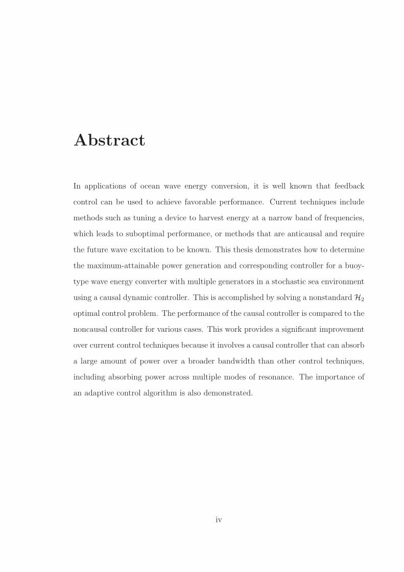
Abstract
In applications of ocean wave energy conversion, it is well known that feedback
control can be used to achieve favorable performance. Current techniques include
methods such as tuning a device to harvest energy at a narrow band of frequencies,
which leads to suboptimal performance, or methods that are anticausal and require
the future wave excitation to be known. This thesis demonstrates how to determine
the maximum-attainable power generation and corresponding controller for a buoy-
type wave energy converter with multiple generators in a stochastic sea environment
using a causal dynamic controller. This is accomplished by solving a nonstandard H2
optimal control problem. The performance of the causal controller is compared to the
noncausal controller for various cases. This work provides a significant improvement
over current control techniques because it involves a causal controller that can absorb
a large amount of power over a broader bandwidth than other control techniques,
including absorbing power across multiple modes of resonance. The importance of
an adaptive control algorithm is also demonstrated.
iv

Contents
Abstract iv
List of Tables vii
List of Figures viii
List of Abbreviations and Symbols x
Acknowledgements xii
1 Introduction 1
1.1 Current technologies . . . . . . . . . . . . . . . . . . . . . . . . . . . 3
1.1.1 Oscillating bodies . . . . . . . . . . . . . . . . . . . . . . . . . 4
1.1.2 Oscillating water columns . . . . . . . . . . . . . . . . . . . . 5
1.1.3 Control algorithms . . . . . . . . . . . . . . . . . . . . . . . . 6
1.2 Overview of thesis work . . . . . . . . . . . . . . . . . . . . . . . . . 7
2 Model Definition 9
2.1 Dynamic model development . . . . . . . . . . . . . . . . . . . . . . . 9
2.2 Hydrodynamic forces . . . . . . . . . . . . . . . . . . . . . . . . . . . 16
2.2.1 Diffraction problem . . . . . . . . . . . . . . . . . . . . . . . . 17
2.2.2 Radiation problem . . . . . . . . . . . . . . . . . . . . . . . . 23
2.3 Sea state characterization . . . . . . . . . . . . . . . . . . . . . . . . 25
2.4 Example WEC design . . . . . . . . . . . . . . . . . . . . . . . . . . 28
2.5 Power generation . . . . . . . . . . . . . . . . . . . . . . . . . . . . . 30
v

3 Optimal Noncausal Performance 33
3.1 Impedance Matched Controller Synthesis . . . . . . . . . . . . . . . . 35
4 Finite-Dimensional Approximation 41
4.1 JONSWAP power spectrum approximation . . . . . . . . . . . . . . . 42
4.2 State-space model identification from frequency domain data . . . . . 43
4.3 Augmented state-spaces . . . . . . . . . . . . . . . . . . . . . . . . . 46
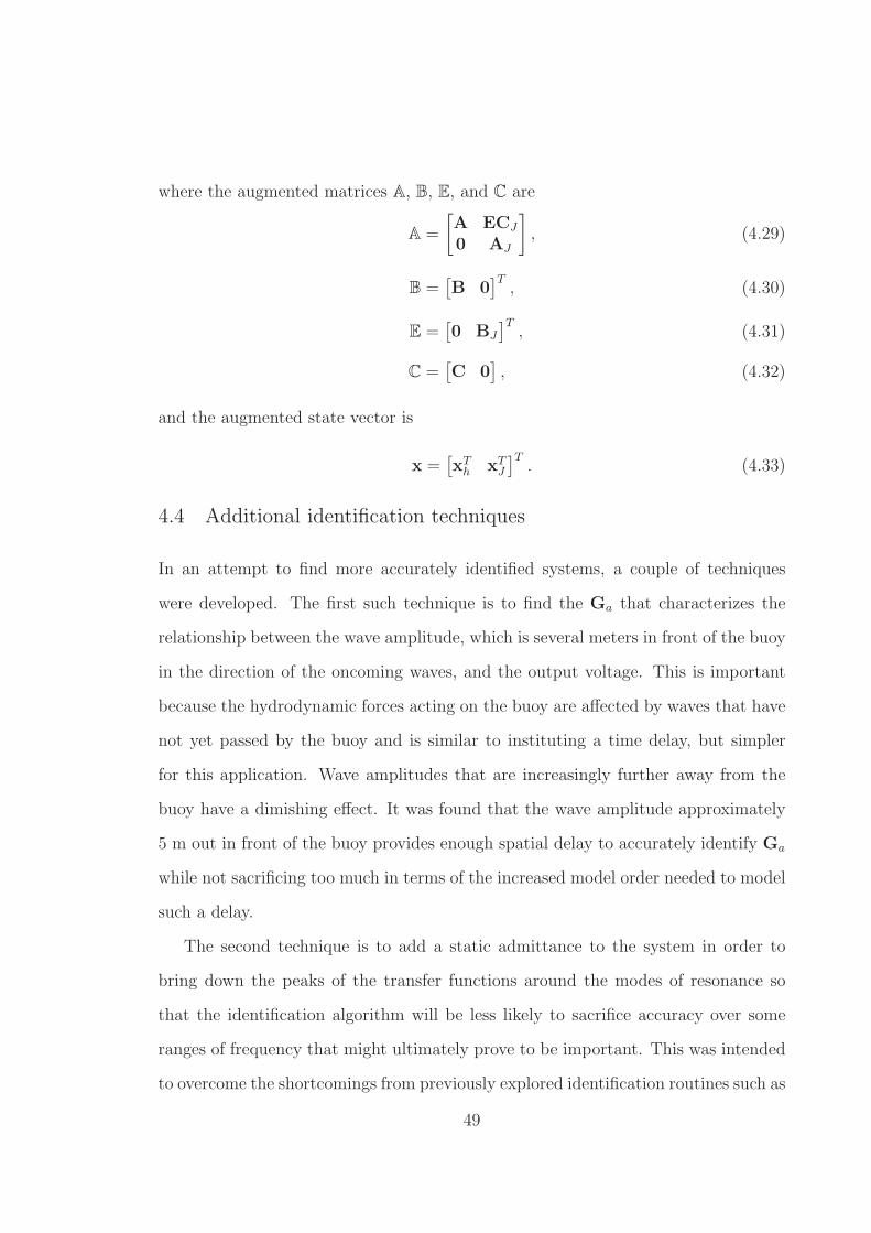
4.4 Additional identification techniques . . . . . . . . . . . . . . . . . . . 49
5 Optimal Causal Performance 51
5.1 Full-state feedback . . . . . . . . . . . . . . . . . . . . . . . . . . . . 52
5.2 Output feedback . . . . . . . . . . . . . . . . . . . . . . . . . . . . . 53
5.3 Simulation . . . . . . . . . . . . . . . . . . . . . . . . . . . . . . . . . 58
6 Adaptive Control 61
6.1 Adaptive control performance . . . . . . . . . . . . . . . . . . . . . . 61
6.2 Future work . . . . . . . . . . . . . . . . . . . . . . . . . . . . . . . . 64
6.2.1 Recursive extended least-squares . . . . . . . . . . . . . . . . 65
7 Conclusions 68
A Static Controller 70
Bibliography 74
vi

List of Tables
2.1 Degrees-of-freedom for buoy. . . . . . . . . . . . . . . . . . . . . . . . 17
2.2 WEC design parameters. . . . . . . . . . . . . . . . . . . . . . . . . . 29
5.1 Average power generation. . . . . . . . . . . . . . . . . . . . . . . . . 58
vii
List of Figures
1.1 Orientations of oscillating body WECs. . . . . . . . . . . . . . . . . . 4
1.2 Conceptual diagram of active control. . . . . . . . . . . . . . . . . . . 7
1.3 General diagram for a WEC. . . . . . . . . . . . . . . . . . . . . . . . 8
2.1 General diagram for a WEC model. . . . . . . . . . . . . . . . . . . . 10
2.2 Hydrodynamic forces and moments. . . . . . . . . . . . . . . . . . . . 18
2.3 Characteristics of a floating cylinder. . . . . . . . . . . . . . . . . . . 18
2.4 JONSWAP power spectra: varying mean wave period. . . . . . . . . . 27
2.5 JONSWAP power spectra: varying sharpness factor. . . . . . . . . . . 27
2.6 General diagram for a WEC with design parameters. . . . . . . . . . 28
2.7 Frequency response for Ga. . . . . . . . . . . . . . . . . . . . . . . . . 30
2.8 Frequency response for Gi. . . . . . . . . . . . . . . . . . . . . . . . . 31
2.9 Feedback control for WEC model. . . . . . . . . . . . . . . . . . . . . 32
3.1 Anticausal harvester power spectra: T1 = 12 s. . . . . . . . . . . . . . 35
3.2 Anticausal harvester power spectra: T1 = 7 s. . . . . . . . . . . . . . 36
3.3 Anticausal harvester power spectra: T1 = 5 s. . . . . . . . . . . . . . 36
4.1 Finite-dimensional approximations for Sa. . . . . . . . . . . . . . . . 44
4.2 Finite-dimensional approximation of Ga. . . . . . . . . . . . . . . . . 47
4.3 Finite-dimensional approximation of Gi. . . . . . . . . . . . . . . . . 48
5.1 Harvester power spectra: T1 = 12 s. . . . . . . . . . . . . . . . . . . . 55
5.2 Harvester power spectra: T1 = 7 s. . . . . . . . . . . . . . . . . . . . 56
viii

5.3 Harvester power spectra: T1 = 5 s. . . . . . . . . . . . . . . . . . . . 57
5.4 Simulated voltage output. . . . . . . . . . . . . . . . . . . . . . . . . 59
5.5 Simulated control current. . . . . . . . . . . . . . . . . . . . . . . . . 59
5.6 Simulated power generation. . . . . . . . . . . . . . . . . . . . . . . . 60
5.7 Simulated energy accumulation. . . . . . . . . . . . . . . . . . . . . . 60
6.1 Adaptive vs. non-adaptive control. . . . . . . . . . . . . . . . . . . . 63
6.2 Conceptual diagram of an indirect STR for a WEC . . . . . . . . . . 64
ix

List of Abbreviations and Symbols
Symbols
Bolded symbols typically denote vectors or matrices. The few symbols that may be
duplicated are put in context where they are used.
a Wave amplitude.
Cc Added damping matrix.
Fa Hydrodynamic force and moment vector.
Ga Transfer function relating wave height (input) to voltage (out-put).
Gi Transfer function relating control current (input) to voltage (out-put).
i Control current (input) vector.
Mc Added mass matrix.
Pgen Average power generation.
R Square matrix with stator resistance values along the diagonal.
Sa Wave height power spectrum.
Sp Harvester power spectrum.
v Voltage (output) vector.
Abbreviations
Below is a non-exhaustive list of abbreviations in this thesis.
JONSWAP Joint North Sea Wave Project (refers to ocean wave spectra).
x

LQG Linear-quadratic-Gaussian.
RELS Recursive extended least-squares.
STR Self-tuning regulator.
WEC Wave energy converter.
xi

Acknowledgements
Thanks are given to Dr. Jeff Scruggs, who advised the work in this thesis and also
chaired the Master’s defense commitee, Dr. Henri Gavin, who provided feedback as
my work progressed and was a member of my Master’s defense committee, and Dr.
Lawrie Virgin, who also served on my committee. Thanks are also given to Dr. Alex
Taflanidis (University of Notre Dame), who provided the initial programming for the
hydrodynamic analysis, and Ian Cassidy, who as a fellow graduate student and friend
helped me search for solutions to research related problems. Finally, thanks are given
to my entire family, especially to my wife Lizzy for providing me with unwavering
support, and my one-and-a-half year-old daughter Isabel, who reminds me to relax
by bringing me my shoes so that I can take her outside to play.
This work was supported by a grants from the Office of Naval Research (Ron
Joslin, Program Officer) and the National Science Foundation - CMMI division -
Control Systems Program (Suhada Jayasuriya, Program Officer), and by the De-
partment of Energy via an SBIR subcontract from Resolute Marine Energy, Inc (Bill
Staby, CEO). This funding is gratefully acknowledged. The statements in this thesis
reflect the views of the author and are not necessarily representative of those of the
sponsors.
xii
1
Introduction
A substantial amount of energy exists in ocean waves. This energy travels over great
distances with relatively small energy losses and is viewed as a potential source of
renewable energy. The power available in ocean waves varies globally and seasonally.
Good locations to harvest energy can provide an average power flux, in terms of power
per meter of wave front, between 20 and 70 kW/m. These locations are usually in
middle to high latitudes and exist primarily on west facing coasts (Barstow et al.
(2008)). It is estimated that each year 2,100 TW-h of wave energy reaches the area
immediately off of the United States coast in locations where the average power flux
exceeds 10 kW/m, which is considered to be the minimal power flux necessary for
wave energy conversion to be worthwhile. Of the total wave energy that reaches U.S.
coastline, it is technologically feasible to harvest approximately 260 TWh which is
about 6% of national energy demand (Bedard et al. (2007)).
Wave power was thrust into the engineering community’s lexicon when much of
the world began looking at energy alternatives in response to the oil crisis of 1973.
It became a popular topic after the concept of converting mechanical energy from
ocean waves into electricity for utility-scale use was promoted in 1974 by Salter
1
(1974). This paper proposes a new device that is now commonly referred to as the
“Salter duck” and defines the problem of ocean wave energy conversion by stating,
“The essential problem is finding a method to convert dispersed, ran-
dom, alternating forces into concentrated, direct force, using a mecha-
nism which is efficient at low levels and yet robust enough to withstand
the worst conditions.”
It can be said that Salter is responsible for creating interest in wave energy
conversion, but modern research in the area has its origins with Yoshio Masuda, a
former Japanese naval commander. Masuda’s studies date back to the 1940s in Japan
where he initiated the scientific pursuit of harvesting energy from ocean waves when
he researched and developed ways to power small-scale navigation buoys (Falcao
(2010)).
Hydrodynamic theory, the crucial foundation of wave energy conversion, was
extensively developed throughout the 20th century due to its relevance in determining
the dynamic motions of ships and forces acting on other structures at sea such as
oil rig platforms. Techniques used to analyze motions of rigid bodies in the presence
of ocean waves include both analytical and numerical methods, the former being
used for simpler geometries and the latter being used for more complex ones. An
example of an analytical technique is found in Hulme (1982) where the profile of
the submerged body is a hemisphere and exists in water of infinite depth. Motion
in both the heave and surge degrees of freedom are considered. Numerical methods
typically involve dividing the body’s surface into individual panels. An example can
be found in Newman (2002). Panel methods are commonly used in the aerospace
industry. A semi-analytical method is provided in Kokkinowrachos et al. (1986) that
can be applied to arbitrary shaped bodies of revolution with vertical axis. This is
accomplished by dividing the body into discrete ring-shaped macroelements of which
2

each element has an analytical solution.
Since the 1970s, much work has been done to determine the amount of power that
exists in ocean waves and many types of wave energy converters (WECs) have been
conceived and developed to some extent including oscillating water columns, surface
floating attenuators, and floating buoy-type point absorbers. Some of these WECs
are now in use, primarily in western Europe (Clement et al. (2002)). But WEC
technology has many challenges that have slowed progress towards a day where large-
scale wave farms are a common source of sustainable electrical energy. Mechanically
speaking, other than developing designs that can efficiently convert mechanical wave
energy into electrical energy, there are survivability issues that arise. Survivability is
even more important for deep water devices where there is higher energy content in
the waves. Despite the demand for environmentally friendly and sustainable sources
of energy, economic and political challenges are also present and difficult to overcome.
These include numerous state and federal regulatory hurdles (especially in the United
States where regulations are outdated and aimed towards conventional hydroelectric
plants) and limited funding for research and development operations (Bedard et al.
(2007)).
Evans (1981) and McCormick (1981) provide extensive overviews that reflect
the state of the art as of the early 1980s when research of WEC technology had
somewhat of a boom period. Relatively recent works that provide a good survey
of where WEC technology stands today include Falcao (2010), Cruz (2008), Falnes
(2002), Salter et al. (2002), Falcao (2004), and Falnes (2007).
1.1 Current technologies
WECs typically fall into one of three categories: oscillating bodies, oscillating water
columns (OWCs), and overtopping devices. Oscillating bodies are floating, articu-
lated structures with transducers, also called power take-off (PTO) systems, installed
3
between degrees of freedom. They absorb wave energy due to dynamic fluid-structure
interaction. OWCs and overtopping devices involve structural installations which are
static. OWCs absorb energy by coupling the resonant oscillation of water elevation
in a submerged air chamber with a gas turbine. Overtopping devices operate on
the same principles as conventional hydropower plants, in which the gravitational
potential energy of water propagating over a device is made to drive a turbine.
1.1.1 Oscillating bodies
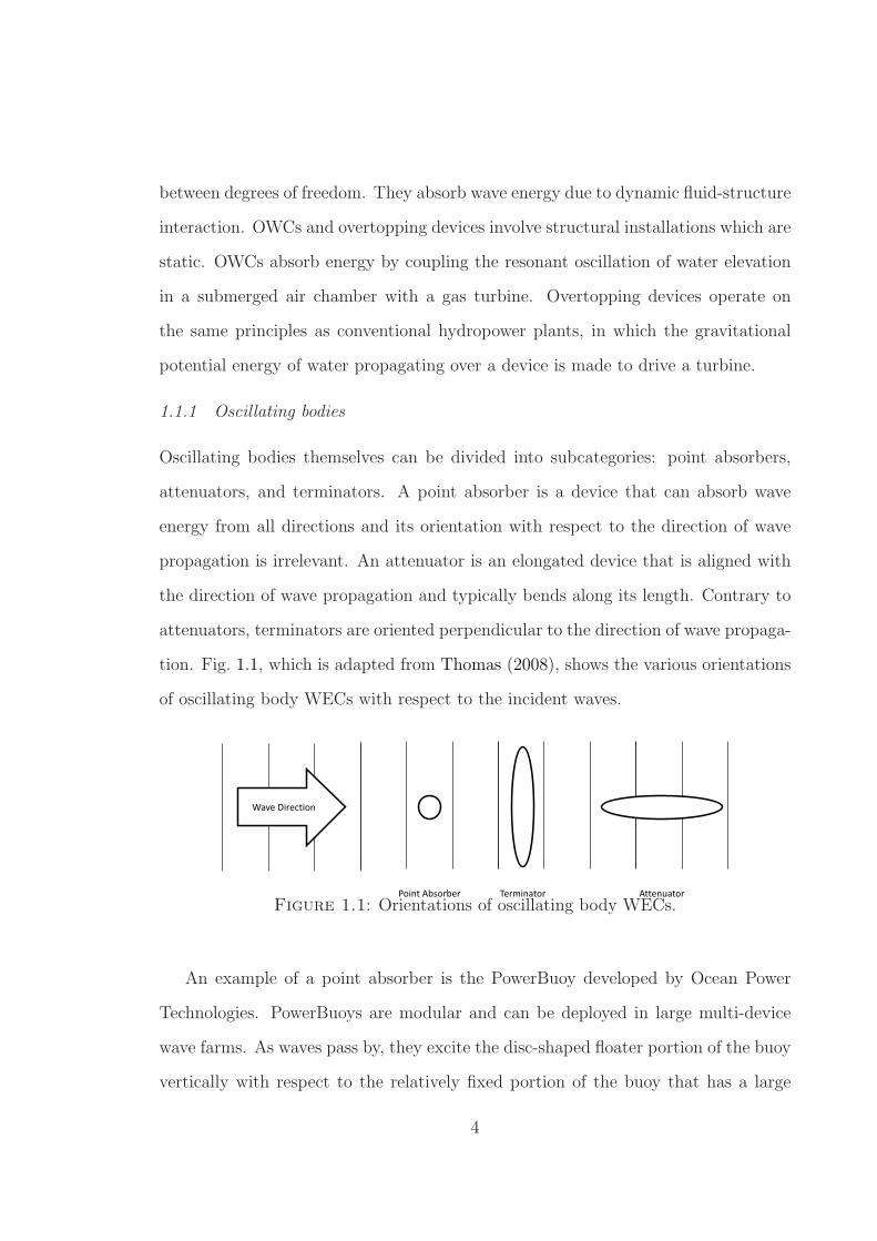
Oscillating bodies themselves can be divided into subcategories: point absorbers,
attenuators, and terminators. A point absorber is a device that can absorb wave
energy from all directions and its orientation with respect to the direction of wave
propagation is irrelevant. An attenuator is an elongated device that is aligned with
the direction of wave propagation and typically bends along its length. Contrary to
attenuators, terminators are oriented perpendicular to the direction of wave propaga-
tion. Fig. 1.1, which is adapted from Thomas (2008), shows the various orientations
of oscillating body WECs with respect to the incident waves.
Figure 1.1: Orientations of oscillating body WECs.
An example of a point absorber is the PowerBuoy developed by Ocean Power
Technologies. PowerBuoys are modular and can be deployed in large multi-device
wave farms. As waves pass by, they excite the disc-shaped floater portion of the buoy
vertically with respect to the relatively fixed portion of the buoy that has a large
4

damping plate and is also moored to the sea floor by a conventional mooring system.
The relative motion of the floater portion moves hydraulic fluid in the buoy that then
spins a generator. The PowerBuoy has undergone sea trials and is currently ready for
market (Unattributed (2011)). Other examples of point absorber oscillating bodies
are the Archimedes Wave Swing (AWS), IPS Buoy, and Wavebob.
An example of an attenuator is the Pelamis WEC developed by Pelamis Wave
Power. Like the PowerBuoy, Pelamis WECs can also be deployed in wave farms and
involves a power hydraulic PTO. The Pelamis WEC is a long articulated structure
that bends at its hinges as waves pass by and this creates pressurized oil that drives
the power hydraulic PTO (Yemm (2008)). The Pelamis has also undergone sea trials
and is deployed off of Scotland and Portugal.
An example of a terminator is the aforementioned Salter Duck. One manifes-
tation of the Salter Duck technology involves a series of floating bodies known as
ducks arranged in a spine and allowed to rotate along the spine independently in
pitch. The dynamics at the joints in between each duck allows for the electronic
control of stiffness, damping, and yielding bending moment with measurement of
bending moment and joint angle (Salter (2008)). This device also has a power hy-
draulic PTO. Extensive tests were done for the device, but due to the politics at
the time, robustness and practicality issues, and controversy over power production
calculations, a full scale device has never gone to sea.
1.1.2 Oscillating water columns
Oscillating water columns (OWCs) can either be fixed structures attached to land
or the sea floor in some fashion or they can be floating structures that are moored
and are relatively static. An OWC consists of a chamber that is filled with air
and exposed to the surface of the water. As a wave passes, it increases the water
height inside the chamber and compresses the air which in turn is forced out through
5
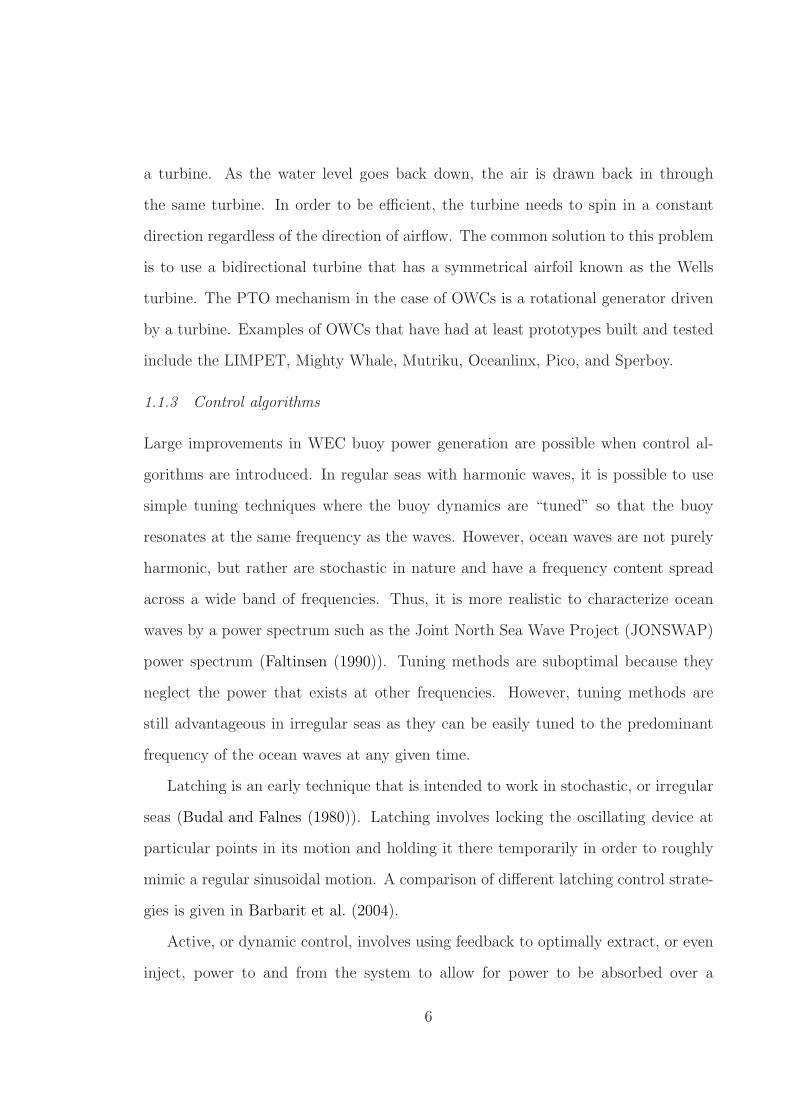
a turbine. As the water level goes back down, the air is drawn back in through
the same turbine. In order to be efficient, the turbine needs to spin in a constant
direction regardless of the direction of airflow. The common solution to this problem
is to use a bidirectional turbine that has a symmetrical airfoil known as the Wells
turbine. The PTO mechanism in the case of OWCs is a rotational generator driven
by a turbine. Examples of OWCs that have had at least prototypes built and tested
include the LIMPET, Mighty Whale, Mutriku, Oceanlinx, Pico, and Sperboy.
1.1.3 Control algorithms
Large improvements in WEC buoy power generation are possible when control al-
gorithms are introduced. In regular seas with harmonic waves, it is possible to use
simple tuning techniques where the buoy dynamics are “tuned” so that the buoy
resonates at the same frequency as the waves. However, ocean waves are not purely
harmonic, but rather are stochastic in nature and have a frequency content spread
across a wide band of frequencies. Thus, it is more realistic to characterize ocean
waves by a power spectrum such as the Joint North Sea Wave Project (JONSWAP)
power spectrum (Faltinsen (1990)). Tuning methods are suboptimal because they
neglect the power that exists at other frequencies. However, tuning methods are
still advantageous in irregular seas as they can be easily tuned to the predominant
frequency of the ocean waves at any given time.
Latching is an early technique that is intended to work in stochastic, or irregular
seas (Budal and Falnes (1980)). Latching involves locking the oscillating device at
particular points in its motion and holding it there temporarily in order to roughly
mimic a regular sinusoidal motion. A comparison of different latching control strate-
gies is given in Barbarit et al. (2004).
Active, or dynamic control, involves using feedback to optimally extract, or even
inject, power to and from the system to allow for power to be absorbed over a
6
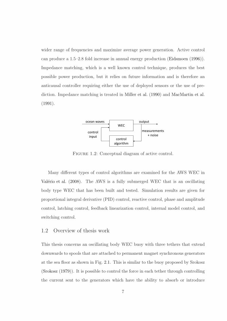
wider range of frequencies and maximize average power generation. Active control
can produce a 1.5–2.8 fold increase in annual energy production (Eidsmoen (1996)).
Impedance matching, which is a well known control technique, produces the best
possible power production, but it relies on future information and is therefore an
anticausal controller requiring either the use of deployed sensors or the use of pre-
diction. Impedance matching is treated in Miller et al. (1990) and MacMartin et al.
(1991).
Figure 1.2: Conceptual diagram of active control.
Many different types of control algorithms are examined for the AWS WEC in
Valerio et al. (2008). The AWS is a fully submerged WEC that is an oscillating
body type WEC that has been built and tested. Simulation results are given for
proportional integral derivative (PID) control, reactive control, phase and amplitude
control, latching control, feedback linearization control, internal model control, and
switching control.
1.2 Overview of thesis work
This thesis concerns an oscillating body WEC buoy with three tethers that extend
downwards to spools that are attached to permanent magnet synchronous generators
at the sea floor as shown in Fig. 2.1. This is similar to the buoy proposed by Srokosz
(Srokosz (1979)). It is possible to control the force in each tether through controlling
the current sent to the generators which have the ability to absorb or introduce
7
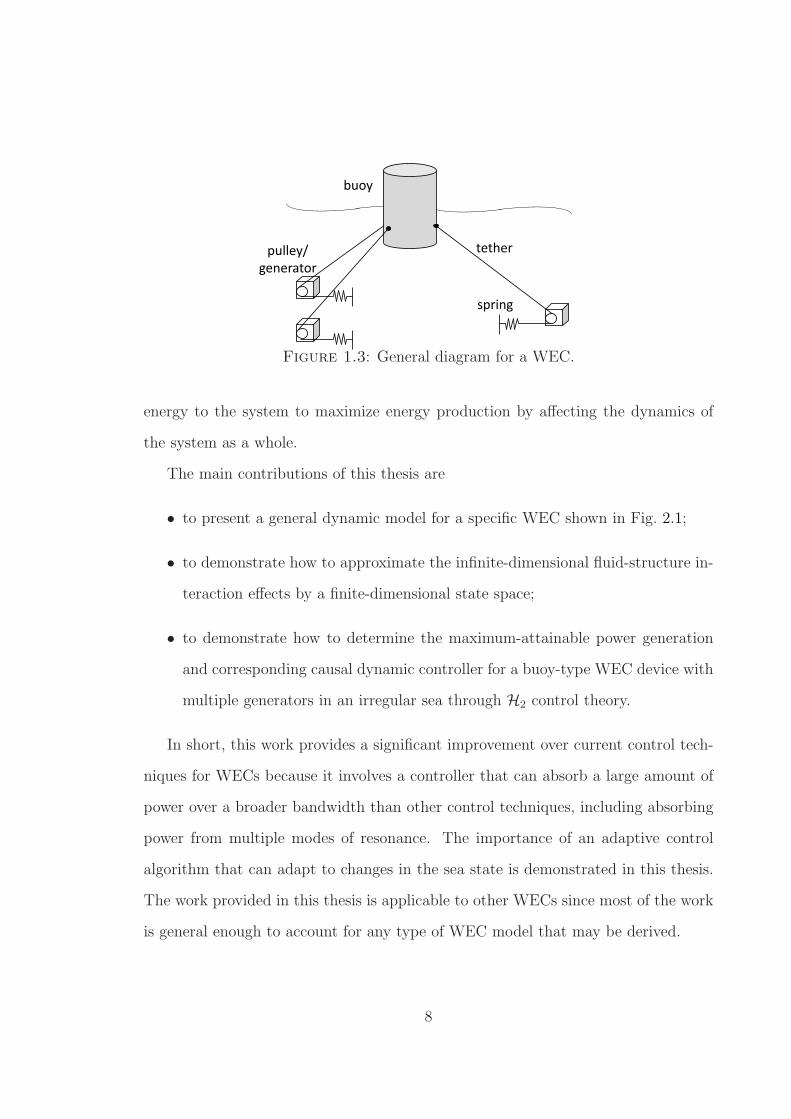
Figure 1.3: General diagram for a WEC.
energy to the system to maximize energy production by affecting the dynamics of
the system as a whole.
The main contributions of this thesis are
• to present a general dynamic model for a specific WEC shown in Fig. 2.1;
• to demonstrate how to approximate the infinite-dimensional fluid-structure in-
teraction effects by a finite-dimensional state space;
• to demonstrate how to determine the maximum-attainable power generation
and corresponding causal dynamic controller for a buoy-type WEC device with
multiple generators in an irregular sea through H2 control theory.
In short, this work provides a significant improvement over current control tech-
niques for WECs because it involves a controller that can absorb a large amount of
power over a broader bandwidth than other control techniques, including absorbing
power from multiple modes of resonance. The importance of an adaptive control
algorithm that can adapt to changes in the sea state is demonstrated in this thesis.
The work provided in this thesis is applicable to other WECs since most of the work
is general enough to account for any type of WEC model that may be derived.
8
2
Model Definition
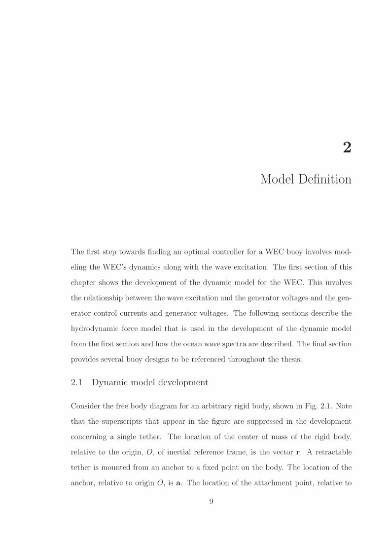
The first step towards finding an optimal controller for a WEC buoy involves mod-
eling the WEC’s dynamics along with the wave excitation. The first section of this
chapter shows the development of the dynamic model for the WEC. This involves
the relationship between the wave excitation and the generator voltages and the gen-
erator control currents and generator voltages. The following sections describe the
hydrodynamic force model that is used in the development of the dynamic model
from the first section and how the ocean wave spectra are described. The final section
provides several buoy designs to be referenced throughout the thesis.
2.1 Dynamic model development
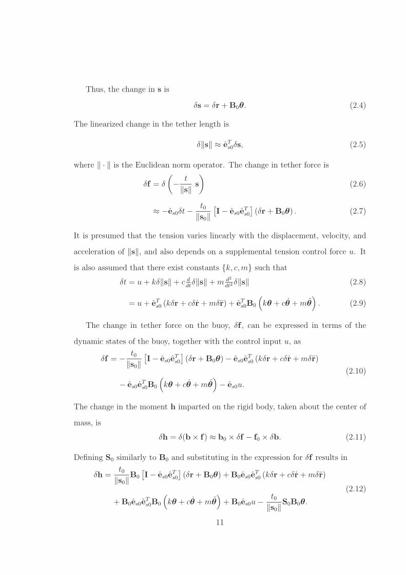
Consider the free body diagram for an arbitrary rigid body, shown in Fig. 2.1. Note
that the superscripts that appear in the figure are suppressed in the development
concerning a single tether. The location of the center of mass of the rigid body,
relative to the origin, O, of inertial reference frame, is the vector r. A retractable
tether is mounted from an anchor to a fixed point on the body. The location of the
anchor, relative to origin O, is a. The location of the attachment point, relative to
9
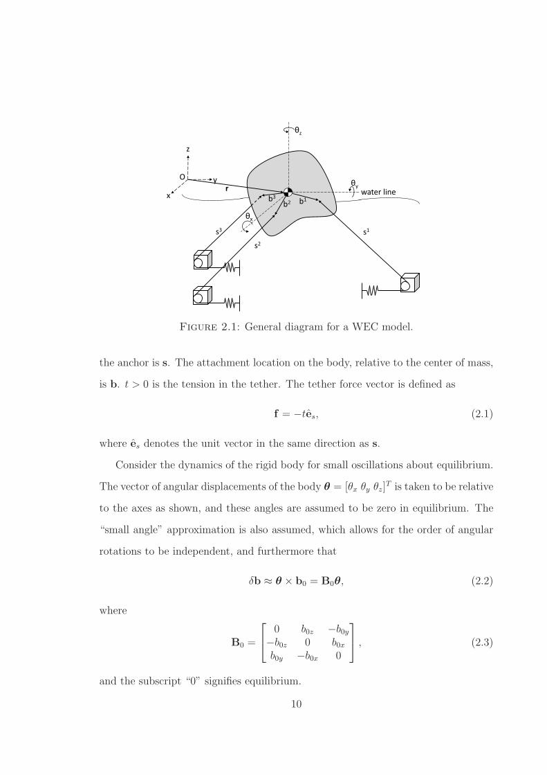
Figure 2.1: General diagram for a WEC model.
the anchor is s. The attachment location on the body, relative to the center of mass,
is b. t > 0 is the tension in the tether. The tether force vector is defined as
f = −tes, (2.1)
where es denotes the unit vector in the same direction as s.
Consider the dynamics of the rigid body for small oscillations about equilibrium.
The vector of angular displacements of the body θ = [θx θy θz]T is taken to be relative
to the axes as shown, and these angles are assumed to be zero in equilibrium. The
“small angle” approximation is also assumed, which allows for the order of angular
rotations to be independent, and furthermore that
δb ≈ θ × b0 = B0θ, (2.2)
where
B0 =
0 b0z −b0y−b0z 0 b0xb0y −b0x 0
, (2.3)
and the subscript “0” signifies equilibrium.
10
Thus, the change in s is
δs = δr+B0θ. (2.4)
The linearized change in the tether length is
δ‖s‖ ≈ eTs0δs, (2.5)
where ‖ · ‖ is the Euclidean norm operator. The change in tether force is
δf = δ
(
− t
‖s‖ s
)
(2.6)
≈ −es0δt−t0
‖s0‖[
I− es0eTs0
]
(δr+B0θ) . (2.7)
It is presumed that the tension varies linearly with the displacement, velocity, and
acceleration of ‖s‖, and also depends on a supplemental tension control force u. It
is also assumed that there exist constants k, c,m such that
δt = u+ kδ‖s‖+ c ddtδ‖s‖+m d2
dt2δ‖s‖ (2.8)
= u+ eTs0 (kδr+ cδr+mδr) + eTs0B0
(
kθ + cθ +mθ
)
. (2.9)
The change in tether force on the buoy, δf , can be expressed in terms of the
dynamic states of the buoy, together with the control input u, as
δf = − t0‖s0‖
[
I− es0eTs0
]
(δr+B0θ)− es0eTs0 (kδr+ cδr+mδr)
− es0eTs0B0
(
kθ + cθ +mθ
)
− es0u.
(2.10)
The change in the moment h imparted on the rigid body, taken about the center of
mass, is
δh = δ(b× f) ≈ b0 × δf − f0 × δb. (2.11)
Defining S0 similarly to B0 and substituting in the expression for δf results in
δh =t0
‖s0‖B0
[
I− es0eTs0
]
(δr+B0θ) +B0es0eTs0 (kδr+ cδr+mδr)
+B0es0eTs0B0
(
kθ + cθ +mθ
)
+B0es0u−t0
‖s0‖S0B0θ.
(2.12)
11
δf and δh can be conveniently represented as
[
δfδh
]
= Gtu−Kt
[
δrθ
]
−Ct
[
δr
θ
]
−Mt
[
δr
θ
]
, (2.13)
where, using the fact that B0 = −BT0 ,
Kt =
[
I
BT0
]
(
kes0eTs0 + γ0
[
I− es0eTs0
]) [
I B0
]
+
[
0 00 γ0S0B0
]
, (2.14)
Ct = c
[
I
BT0
]
es0eTs0
[
I B0
]
, (2.15)
Mt = m
[
I
BT0
]
es0eTs0
[
I B0
]
, (2.16)
Gt = −[
I
BT0
]
es0, (2.17)
and where γ0 = t0/‖s0‖.
Now, consider a buoy with N tethers. For an arbitrary amount of tethers, the
total dynamic component of the force and moment on the buoy is
[
δfδh
]
=
[
δfwδhw
]
+
[
δf1 + . . .+ δfN
δh1 + . . .+ δhN
]
(2.18)
=
[
δfwδhw
]
− Kt
[
δrθ
]
− Ct
[
δr
θ
]
− Mt
[
δr
θ
]
+[
G1t . . . GN
t
]
u, (2.19)
where
u =[
u1 . . . uN]T, (2.20)
and
Kt =N∑
i=1
Kit, (2.21)
12
and Ct and Mt are defined similar to Kt. Interestingly, we note that for any vector q
N∑
i=1
γ0Si0B
i0q =
N∑
i=1
−(q× bi0)× f i0 (2.22)
=N∑
i=1
−q× (bi0 × f i0) (2.23)
= −q×(
N∑
i=1
bi0 × f i0
)
. (2.24)
In static equilibrium, the term in the parentheses is the sum of moments acting on the
buoy by the tethers. Assuming no other moments act on the buoy static equilibrium,
it can be concluded that the above term will be zero for all q, implying that
N∑
i=1
γ0Si0B
i0 = 0. (2.25)
As such, the γi0Si0B
i0 terms in each Ki
t cancel out.
Regarding the wave forces and moments, they are presumed to be of the form
[
δfwδhw
]
=
[
δfaδha
]
+
[
δfbδhb
]
+
[
δfcδhc
]
, (2.26)
where δfa, δha are the force and moment imparted on the buoy by the wave,
δfb, δhb are the force and moment due to buoyancy, δfc, δhc are the hydrodynamic
(i.e. added mass and damping) forces.
Let the Fourier transforms of δfa, δha be denoted F(δfa) and F(δha). It is
presumed that there is a 6 × 1 transfer function matrix Fa(jω) relating the wave
amplitude a to these forces and moments, i.e.
[
F(δfa)F(δha)
]
= Fa(jω)F(a). (2.27)
13
Determining Fa(jω) involves solving a frequency dependent partial differential equa-
tion for a fluid-structure interaction problem which does not produce a rational trans-
fer function. The resulting transfer function is infinite-dimensional, but it is possible
to find series solutions for different shapes and levels of accuracy (Kokkinowrachos et al.
(1986)). This is discussed in the following section.
The change in hydrostatic buoyancy force δfb and moment δhb (relative to equi-
librium) are always linearly related to the displacements δr and δθ via a buoyancy
stiffness matrix Kb, i.e.[
δfbδhb
]
= −Kb
[
δrδθ
]
. (2.28)
The particular components of Kb will vary with the buoy shape. Kb can be de-
termined by linearizing the stiffness about the center of mass of the static buoy at
equilibrium.
Let the Fourier transforms of δfc, δhc be denoted F (δfc) and F (δhc). Then it
is presumed that
[
F (δfc)F (δhc)
]
= − [jωMc(ω) +Cc(ω)]
[
F (δr)
F(θ)
]
, (2.29)
where Mc(ω) and Cc(ω) are the added mass and damping matrices respectively.
These are challenging to determine for the same reasons given for Fa(jω) and solu-
tions can also be found. This is also discussed in the following section.
It is also known that[
µI 0
0 J
] [
δr
θ
]
=
[
δfδh
]
, (2.30)
where µ is the mass of the buoy and J is the rotational inertia matrix. Thus, the
equation of motion becomes
([
µI 0
0 J
]
+ Mt
)[
δr
θ
]
=
[
δfwδhw
]
− Kt
[
δrθ
]
− Ct
[
δr
θ
]
+[
G1t . . . GN
t
]
u. (2.31)
14
Bringing these definitions into the differential equation of motion gives the full
dynamics of the system by the following pair of equations:
([
µI 0
0 J
]
+ Mt
)[
δr
θ
]
=
[
δfaδha
]
+
[
δfcδhc
]
−(
Kb + Kt
)
[
δrθ
]
− Ct
[
δr
θ
]
+[
G1t . . . GN
t
]
u,
(2.32)
[
F (δfc)F (δhc)
]
= − [jωMc(ω) +Cc(ω)]
[
F (δr)
F(θ)
]
. (2.33)
Putting everything in the frequency domain and recognizing that F(δr) = (jω)−1F(δr)
and F(δr) = jωF(δr) (and similarly for F(θ) and F(θ)), the above is
[
jω
([
µI 0
0 J
]
+Mc(ω) + Mt
)
+(
Cc(ω) + Ct
)
+1
jω
(
Kb + Kt
)
]
[
F(δr)
F(θ)
]
= Fa(jω)F(a) +[
G1t . . . GN
t
]
F (u) .
(2.34)
The voltage vector resulting from the tether extension velocity can be defined as
v = Ked
dt
[
δ‖s1‖ . . . δ‖sN‖]T, (2.35)
where Ke is the resulting linear back EMF constant from the generator and pulley.
Then from (2.5), it is known that
v = KeL
[
δr
δθ
]
, (2.36)
where
L = −[
G1t . . . GN
t
]T. (2.37)
Multiplying (2.34) through by the inverse of the matrix in the brackets, i.e.
W(jω) = jω
([
µI 0
0 J
]
+Mc(ω) + Mt
)
+(
Cc(ω) + Ct
)
+1
jω
(
Kb + Kt
)
, (2.38)
15
and multiplying by L, gives the transfer functions from the wave amplitude, a and
the control input current i = −(1/Ke)u, to the generator voltages, v, which have
the form
F(v) = Ga(jω)F(a) +Gi(jω)F(i), (2.39)
where
Ga(jω) = KeLW−1(jω)Fa(jω), (2.40)
Gi(jω) = K2eLW
−1(jω)LT . (2.41)
Figs. 2.7 and 2.8 show Ga(jω) and Gi(jω) for the WEC provided in Table 2.2.
2.2 Hydrodynamic forces
The buoy model derived in the previous section is not complete without the infinite-
dimensional functions, Fa(jω), Mc(ω), and Cc(ω), which describe the hydrodynamic
forces and moments, added mass, and added damping acting in each of the degrees-
of-freedom of the buoy in space. The term “added mass” refers to the mass associated
with the displaced volume of water as the buoy portion of the WEC moves, as there
is a volume of water that must move when the buoy moves. Similarly, the term
“added damping” refers to the additional amount of damping that occurs because
of the movement of the same volume of water. There are many ways to determine
these functions for various body shapes. For simpler shapes there are often analytical
solutions, but numerical techniques exist that are able to handle arbitrary shapes and
can typically be found in commercial software packages.
A semi-analytical approach relevant to large bodies of revolution with a vertical
axis and finite water depth can be found in Kokkinowrachos et al. (1986) and was
used for the hydrodynamic analysis of the cylinder portion of the WEC. The method
is based on the discretization of the flow field around the structure using coaxial ring
elements, which in the case of the cylindrical buoy in this thesis is a single element.
16

Table 2.1: Degrees-of-freedom for buoy.
DOF Motion1 translation in x (surge)2 translation in y (sway)3 translation in z (heave)4 rotation about x (roll)5 rotation about y (pitch)6 rotation about z (yaw)
The velocity potential in each element is approximated by a Fourier series and both
the so-called diffraction (i.e. concerning the diffraction of the incident wave) and
radiation (i.e. concerning the oscillations of the buoy) problems are solved. The
cylindrical body of arbitrary dimensions to be considered is shown in Fig. 2.2 and
the forces and moments acting on the body, which is oscillating in several degrees-
of-freedom, are assumed to be equivalent to the forces that would act on it if it were
constrained in its position. Table 2.1 lists the degrees-of-freedom (DOF) of the buoy.
Note that the momentM6 will be zero since motion in that degree of freedom cannot
be induced due to symmetry. Additionally, the components of the added mass and
added damping matrices corresponding to the same degree of freedom will be zero.
The infinite-dimensional functions, Fa(jω), Mc(ω), and Cc(ω), which describe the
hydrodynamic forces and moments, added mass, and added damping acting in each
of the degrees-of-freedom of the buoy in space, can be determined using the material
in the following subsections. Parameters relevant to the geometry of the diffraction
and radiation problems are shown in Fig. 2.3.
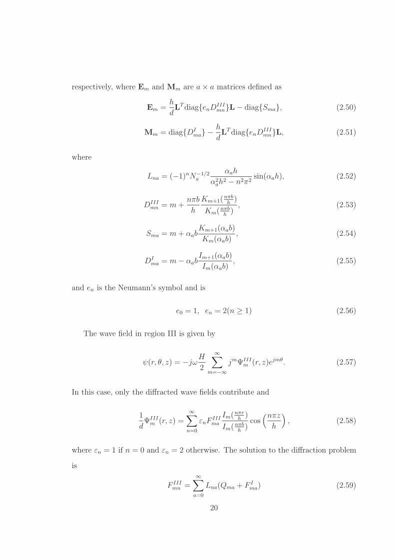
2.2.1 Diffraction problem
The total velocity potential of the flow field around the cylinder is the superposition
of the incident and diffracted wave fields, which in cylindrical coordinates is expressed
as
ψ(r, θ, z) = ψI(r, θ, z) + ψB(r, θ, z), (2.42)
17
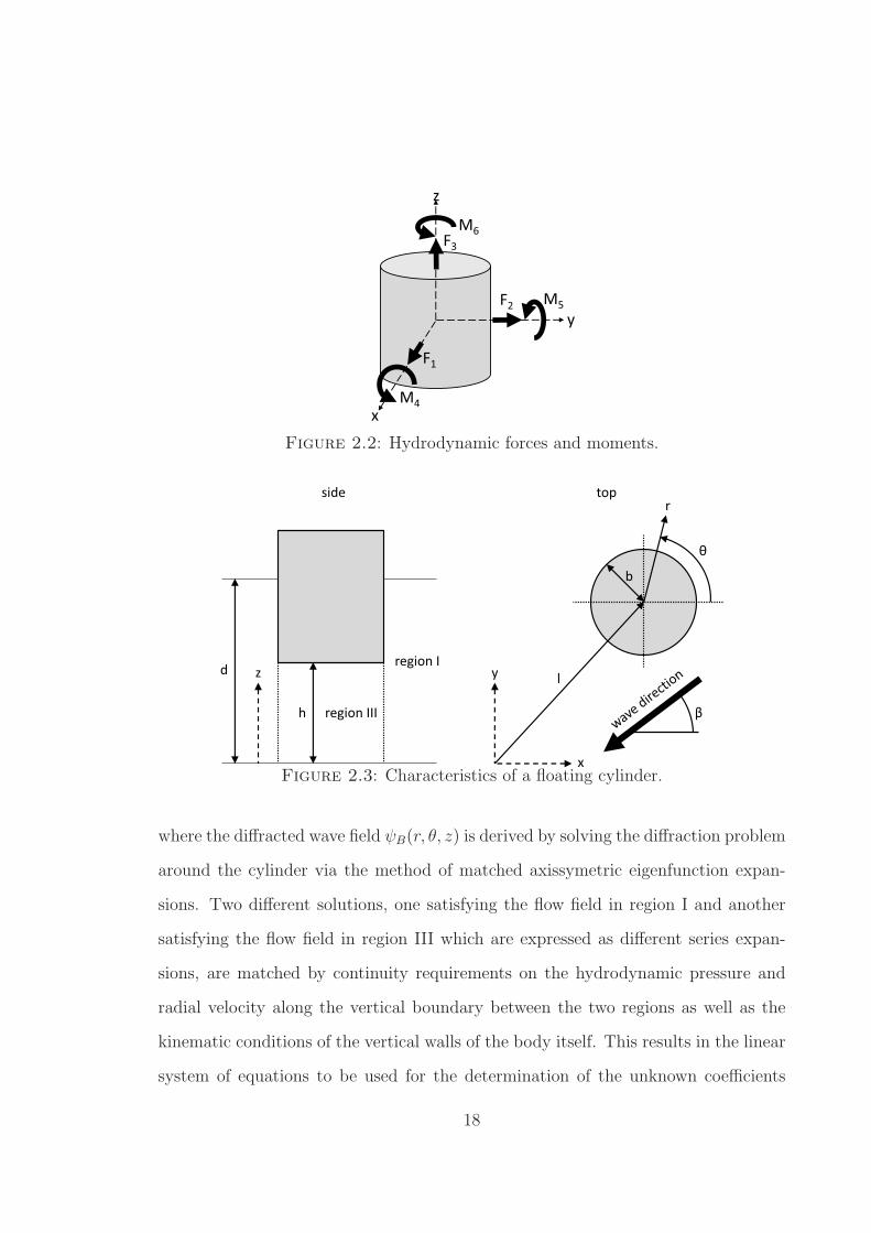
Figure 2.2: Hydrodynamic forces and moments.
Figure 2.3: Characteristics of a floating cylinder.
where the diffracted wave field ψB(r, θ, z) is derived by solving the diffraction problem
around the cylinder via the method of matched axissymetric eigenfunction expan-
sions. Two different solutions, one satisfying the flow field in region I and another
satisfying the flow field in region III which are expressed as different series expan-
sions, are matched by continuity requirements on the hydrodynamic pressure and
radial velocity along the vertical boundary between the two regions as well as the
kinematic conditions of the vertical walls of the body itself. This results in the linear
system of equations to be used for the determination of the unknown coefficients
18
needed for the representation of the velocity potential in each fluid region.
The total wave field in region I is given by
ψ(r, θ, z) = −jωH2
∞∑
m=−∞
jmΨIm(r, z)e
jmθ, (2.43)
where H is the wave height and
1
dΨI
m(r, z) =∞∑
a=0
(
QmaIm(αar)
Im(αab)+ F I
ma
Km(αar)
Km(αab)
)
Za(z), (2.44)
where Im(·) denotes the modified Bessel function of the second kind, αa a ∈ 1, . . .
being the real solutions of the transcendental equation
ω2
g+ αa tan(αad) = 0, (2.45)
and α0 = −jk, where k is the solution of the dispersion relationship
ω2
g+ k tanh(kd) = 0. (2.46)
The orthogonal function Za(z) in (2.44) is given by
Za(z) =1
2
(
1 +sin(2αad)
2αad
)−1/2
cos(αaz). (2.47)
In (2.44), Qma is the coefficient for the wave field created by the incident wave whereas
F Ima is the coefficient for the diffracted wave field around the body, i.e. region I, and
are
Qma = jmejkl cos(θ0 − β)e−jmβ
dZ ′0(d)
Im(αab)δ0a, (2.48)
F Ima = E−1
m MmQma, (2.49)
19
respectively, where Em and Mm are a× a matrices defined as
Em =h
dLTdiagenDIII
mnL− diagSma, (2.50)
Mm = diagDIma −
h
dLTdiagenDIII
mnL, (2.51)
where
Lna = (−1)nN−1/2a
αah
α2ah
2 − n2π2sin(αah), (2.52)
DIIImn = m+
nπb
h
Km+1(nπbh)
Km(nπbh), (2.53)
Sma = m+ αabKm+1(αab)
Km(αab), (2.54)
DIma = m− αab
Im+1(αab)
Im(αab), (2.55)
and en is the Neumann’s symbol and is
e0 = 1, en = 2(n ≥ 1) (2.56)
The wave field in region III is given by
ψ(r, θ, z) = −jωH2
∞∑
m=−∞
jmΨIIIm (r, z)ejmθ. (2.57)
In this case, only the diffracted wave fields contribute and
1
dΨIII
m (r, z) =∞∑
n=0
εnFIIIma
Im(nπrh)
Im(nπbh)cos(nπz
h
)
, (2.58)
where εn = 1 if n = 0 and εn = 2 otherwise. The solution to the diffraction problem
is
F IIImn =
∞∑
a=0
Lna(Qma + F Ima) (2.59)
20
The hydrodynamic forces and moments acting on the cylindrical body are given
by the integration of the pressure field around the body over the mean wetted surface
S as
Ft = −∫ ∫
S
jωρψe−jωtndS = Fe−jωt, (2.60)
Mt = −∫ ∫
S
jωρψe−jωt(r× n)dS =Me−jωt, (2.61)
where
F = −ρω2H
2
∫ ∫
S
∞∑
m=−∞
jmΨm(r, z)ejmθndS, (2.62)
M = −ρω2H
2
∫ ∫
S
∞∑
m=−∞
jmΨm(r, z)ejmθ(r× n)dS, (2.63)
where r denotes the position vector extending from the reference point of forces and
moments to each point on S and n is the unit normal vector of the body’s wetted
surface in average position pointing outwards. Let Fq q ∈ 1, 2, 3 and Mq q ∈ 4, 5
denote the force and moment, respectively, along the qth degree of freedom and Mkq
k ∈ 1, 2, 3 be the contribution to the moment Mq of the force acting along the kth
degree of freedom so that
M5 =M15 +M3
5 , (2.64)
M4 =M24 +M3
4 . (2.65)
21
Evaluation of the integrals in (2.62) and (2.63) is straightforward and leads to
F1 = ρω2H
2d
∑
m∈−1,1
πjm∞∑
a=0
I1a(Qma + F Ima), (2.66)
M15 = −ρω2H
2d
∑
m∈−1,1
πjm∞∑
a=0
I15a(Qma + F Ima), (2.67)
F2 = ρω2H
2d
∑
m∈−1,1
πjm+1
∞∑
a=0
I1a(Qma + F Ima), (2.68)
M24 = ρω2H
2d
∑
m∈−1,1
πjm+1
∞∑
a=0
I5a(Qma + F Ima), (2.69)
F3 = ρω2H
2d2π
(
b
2F III00 +
∞∑
n=0
I3nFIII0n
)
, (2.70)
M35 = −ρω2H
2d
∑
m∈−1,1
πjm
(
1
4b3F III
m0 +∞∑
n=1
I35nFIIImn
)
, (2.71)
M34 = ρω2H
2d
∑
m∈−1,1
πmjm+1
(
1
2b3F III
m0 +∞∑
n=1
I35nFIIImn
)
, (2.72)
where
I1a = b (sin(αad)− sin(αah))1
αa
N−1/2a , (2.73)
I3n = 2nπbI1
(
nπbh
)
hI0(
nπbh
)
h2
n2π2cos(nπ), (2.74)
I35a = b1
αa
N−1/2a
(
1
αa
(cos(αad)− cos(αah)) + (d− p) sin(αad)− (h− p) sin(αah)
)
,
(2.75)
I35n = 2bh2
n2πcos(nπ)
(
m+nπbIm+1
(
nπbh
)
hIm(
nπbh
) − 1
)
, (2.76)
and p is the position of the point with respect to which the moments are calculated.
22
The hydrodynamic force and moment matrix Fa(jω) is constucted as
Fa(jω) =[
F1(jω) F2(jω) F3(jω) M4(jω) M5(jω) 0]T. (2.77)
2.2.2 Radiation problem
The cylinder is now assumed to vibrate in its qth mode with amplitude ξq in still
water of depth d. The velocity potential of the radiated wave due to the vibration
of the body in the qth direction is
ψR,q(r, θ, z) = −jωξq∞∑
m=−∞
Ψm,q(r, z)ejmθ, (2.78)
where the unknowns Ψm,q can be derived by the method of matched eigenfunction
expansions previously discussed for the diffraction problem. The solution for region
I is expressed by
1
δqΨI
qm =∞∑
a=0
F Iq,ma
Km(αar)
Km(αab)Za(z), (2.79)
and the solution for region III is
1
δqΨIII
qm (r, z) = gqm(r, z) +∞∑
n=0
εnFIIIq,ma
Im(
nπrh
)
Im(
nπbh
) cos(nπz
h
)
(2.80)
where δq = d for q ∈ 1, 2, 3 and δq = d2 for q ∈ 4, 5 and
F Iq,ma = E−1
m
(
Pq,ma −h
dLandiagenDIII
mnQTj,mn
)
, (2.81)
F IIIq,ma =
∞∑
a=0
Lna(Fma) +Qq,mn, (2.82)
g3m(r, z) =z2 − 1
2r2
2hd; m = 0, (2.83)
g5m(r, z) = −rz2 + 1
4r3
4hd2; m ∈ −1, 1, (2.84)
g4m(r, z) = jmg5m(r, z); m ∈ −1, 1. (2.85)
23
The hydrodynamic forces and moments acting on the body are given by the
integration of the pressure field around the body over the mean wetted surface S.
Fpq = −∫ ∫
S
jωρψqe−jωtnpdS = fpqe
−jωtξq, (2.86)
where
fpq = −ρω2
∫ ∫
S
∞∑
m=−∞
Ψj,m(r, z)ejmθnpdS, (2.87)
and the generalized normal component np is
n1 = n2 = n3 ≡ n, (2.88)
n4 = n5 ≡ r× n. (2.89)
Force fpq may be expressed in terms of added mass mpq and added damping coeffi-
cients cpq as
fpq(jω) = ω2
(
mpq +j
ωcpq
)
. (2.90)
Equating the real and imaginary parts of (2.87) and (2.90) leads to the calculation
of mpq(ω) and cpq(ω) which are the (p, q)th components of the added mass matrix
Mc(ω) and added damping matrix Cc(ω) respectively. The integrals in (2.87) lead
24
to
f1q = ρω2δq∑
m∈−1,1
π∞∑
a=0
I1a(
Qq,ma + F Iq,ma
)
, (2.91)
f 15q = −ρω2δq
∑
m∈−1,1
π∞∑
a=0
I15a(
Qq,ma + F Iq,ma
)
, (2.92)
f2q = ρω2δq∑
m∈−1,1
mπj∞∑
a=0
I1a(
Qq,ma + F Iq,ma
)
, (2.93)
f 14q = ρω2δq
∑
m∈−1,1
mπj∞∑
a=0
I15a(
Qq,ma + F Iq,ma
)
, (2.94)
f3q = ρω2δq
(
πbF IIIj,00 +
∞∑
n=0
I3nFIIIj,0n
)
, (2.95)
f 35q = −ρω2δq
(
π
4b3F III
m0 +∞∑
n=1
I35nFIIIq,mn
)
, (2.96)
f 34q = ρω2δqmj
(
π
2b3F III
j,m0 +∞∑
n=1
I35nFIIIq,mn
)
, (2.97)
with
f5q = f 15q + f 3
5q, (2.98)
f4q = f 24q + f 3
4q. (2.99)
For the analysis in this thesis, the truncation of the infinite series for region
I, region III, and the diffraction problem are 10, 25, and 10 respectively. These
truncations are done at sufficiently large values where the solution does not change
dramatically by including additional terms in the series.
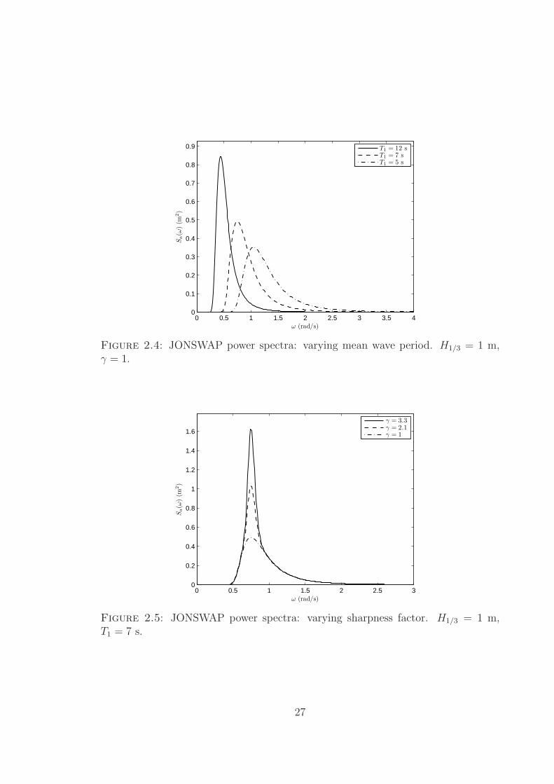
2.3 Sea state characterization
Unlike other examples that can be found in literature concerning WECs that treat
ocean waves as being purely harmonic, this thesis models the ocean wave distur-
25
bance as having frequency content spread across a wide band of frequencies. This is
consistent with reality and is important since a good WEC should be able to absorb
as much power as possible and if significant power is available over a wide range of
frequencies then it should be exploited.
We assume the wave height (i.e. trough to crest height) a(t) to be a stationary
stochastic process with spectral density Sa(ω), and with the normalization convention
that the standard deviation of a(t) is
σ2 =1
2π
∫ ∞
−∞
Sa(ω)dω, (2.100)
where the frequency ω is in rad/s.
In ocean engineering, one of the most widely-used functions for Sa(ω) is the
JONSWAP power spectrum, parametrized by its mean wave period T1, significant
wave heigh H1/3, and sharpness factor γ (Faltinsen (1990)). The spectrum is found,
in terms of these parameters, as
Sa(ω) = 310πH2
1/3
T 41ω
5exp
[−944
T 41ω
4
]
γY , (2.101)
where
Y = exp
[
−(
0.191ωT1 − 1√2φ
)2]
, (2.102)
and
φ =
0.07 : ω ≤ 5.240.09 : ω > 5.24
(2.103)
The sharpness factor γ is constrained to be between 1 and 3.3, the former describ-
ing what is known as a fully developed sea state, which has a wider bandwidth of
frequency content, and the latter providing a spectrum with a high quality factor,
or a narrower band of excitation. Some Examples of JONSWAP power spectra are
shown in Figs. 2.4 and 2.5.
26
0 0.5 1 1.5 2 2.5 3 3.5 40
0.1
0.2
0.3
0.4
0.5
0.6
0.7
0.8
0.9
ω (rad/s)
Sa(ω
)(m
2)
T1 = 12 sT1 = 7 sT1 = 5 s
Figure 2.4: JONSWAP power spectra: varying mean wave period. H1/3 = 1 m,γ = 1.
0 0.5 1 1.5 2 2.5 30
0.2
0.4
0.6
0.8
1
1.2
1.4
1.6
ω (rad/s)
Sa(ω
)(m
2)
γ = 3.3γ = 2.1γ = 1
Figure 2.5: JONSWAP power spectra: varying sharpness factor. H1/3 = 1 m,T1 = 7 s.
27
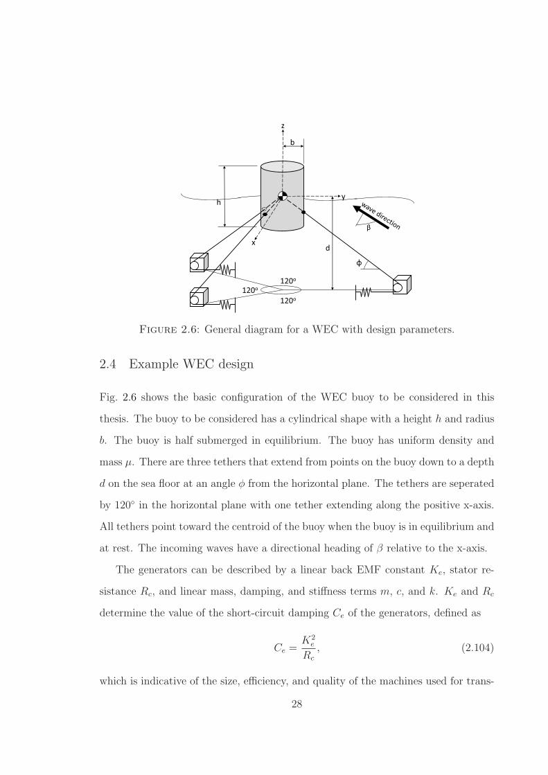
Figure 2.6: General diagram for a WEC with design parameters.
2.4 Example WEC design
Fig. 2.6 shows the basic configuration of the WEC buoy to be considered in this
thesis. The buoy to be considered has a cylindrical shape with a height h and radius
b. The buoy is half submerged in equilibrium. The buoy has uniform density and
mass µ. There are three tethers that extend from points on the buoy down to a depth
d on the sea floor at an angle φ from the horizontal plane. The tethers are seperated
by 120 in the horizontal plane with one tether extending along the positive x-axis.
All tethers point toward the centroid of the buoy when the buoy is in equilibrium and
at rest. The incoming waves have a directional heading of β relative to the x-axis.
The generators can be described by a linear back EMF constant Ke, stator re-
sistance Rc, and linear mass, damping, and stiffness terms m, c, and k. Ke and Rc
determine the value of the short-circuit damping Ce of the generators, defined as
Ce =K2
e
Rc
, (2.104)
which is indicative of the size, efficiency, and quality of the machines used for trans-
28
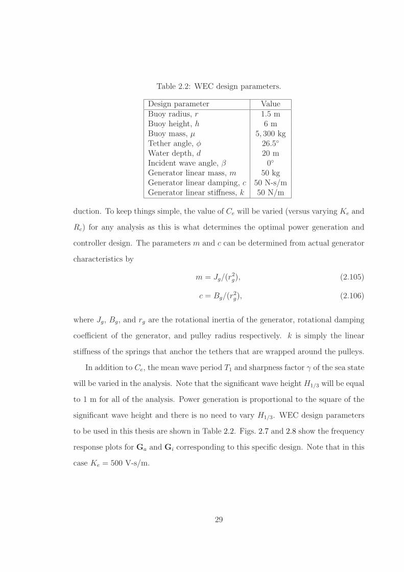
Table 2.2: WEC design parameters.
Design parameter ValueBuoy radius, r 1.5 mBuoy height, h 6 mBuoy mass, µ 5, 300 kgTether angle, φ 26.5
Water depth, d 20 mIncident wave angle, β 0
Generator linear mass, m 50 kgGenerator linear damping, c 50 N-s/mGenerator linear stiffness, k 50 N/m
duction. To keep things simple, the value of Ce will be varied (versus varying Ke and
Rc) for any analysis as this is what determines the optimal power generation and
controller design. The parameters m and c can be determined from actual generator
characteristics by
m = Jg/(r2g), (2.105)
c = Bg/(r2g), (2.106)
where Jg, Bg, and rg are the rotational inertia of the generator, rotational damping
coefficient of the generator, and pulley radius respectively. k is simply the linear
stiffness of the springs that anchor the tethers that are wrapped around the pulleys.
In addition to Ce, the mean wave period T1 and sharpness factor γ of the sea state
will be varied in the analysis. Note that the significant wave height H1/3 will be equal
to 1 m for all of the analysis. Power generation is proportional to the square of the
significant wave height and there is no need to vary H1/3. WEC design parameters
to be used in this thesis are shown in Table 2.2. Figs. 2.7 and 2.8 show the frequency
response plots for Ga and Gi corresponding to this specific design. Note that in this
case Ke = 500 V-s/m.
29
0 0.5 1 1.5 2 2.5 3 3.5 4
102
104
106
‖G
a(j
ω)‖
(V/m
)
Ga,1
Ga,2 and Ga,3
0 0.5 1 1.5 2 2.5 3 3.5 4−20
−15
−10
−5
0
5
ω (rad/s)
<G
a(j
ω)
(rad)
Figure 2.7: Frequency response for Ga.
2.5 Power generation
The purpose of developing a model of the WEC is to test its performance in terms
of power generation, specifically when it uses an active control law. In general,
the WEC should be able to harvest more power on average when it has better
generator efficiency, or larger values of Ce. A WEC with large values of Ce will be
able to apply larger currents to the generators without experiencing large losses due
to internal resistances, otherwise known as “i2R” losses. In addition to values for
Ce, the characterisics of the ocean wave power spectrum will affect power generation
greatly. As previously mentioned, power generation will scale up proportionally to
H21/3. Unlike in most WECs which absorb power from a small band of frequencies
around a single mode of resonance, power generation should not be as sensitive to
T1 since the active controller should be able to absorb power over multiple modes of
30

0 0.5 1 1.5 2 2.5 3 3.5 4
100
101
102
103
104
‖G
i(j
ω)‖
(V/A
)
Gi,11, Gi,22, and Gi,33
Gi,12, Gi,13, and Gi,23
0 0.5 1 1.5 2 2.5 3 3.5 4
−4
−2
0
2
4
6
8
ω (rad/s)
<G
i(j
ω)
(rad)
Figure 2.8: Frequency response for Gi.
resonance. As is evident from the frequency response plots of Ga and Gi, there are
three distinct modes of resonance for this WEC. By looking at the relative phases
between different generator voltages which are proportional to the velocity of the
tethers, it is possible to tell that the modes of resonance are ordered as surge/sway,
pitch/roll, and heave in order from lowest to highest frequency.
A general diagram of a WEC with a control algorithm is shown in Fig. 1.3. A
more specific diagram showing the WEC with an active control law to be examined
in this thesis is shown in Fig. 2.9. The controller is to be designed to maximize the
average power generation over time.
31
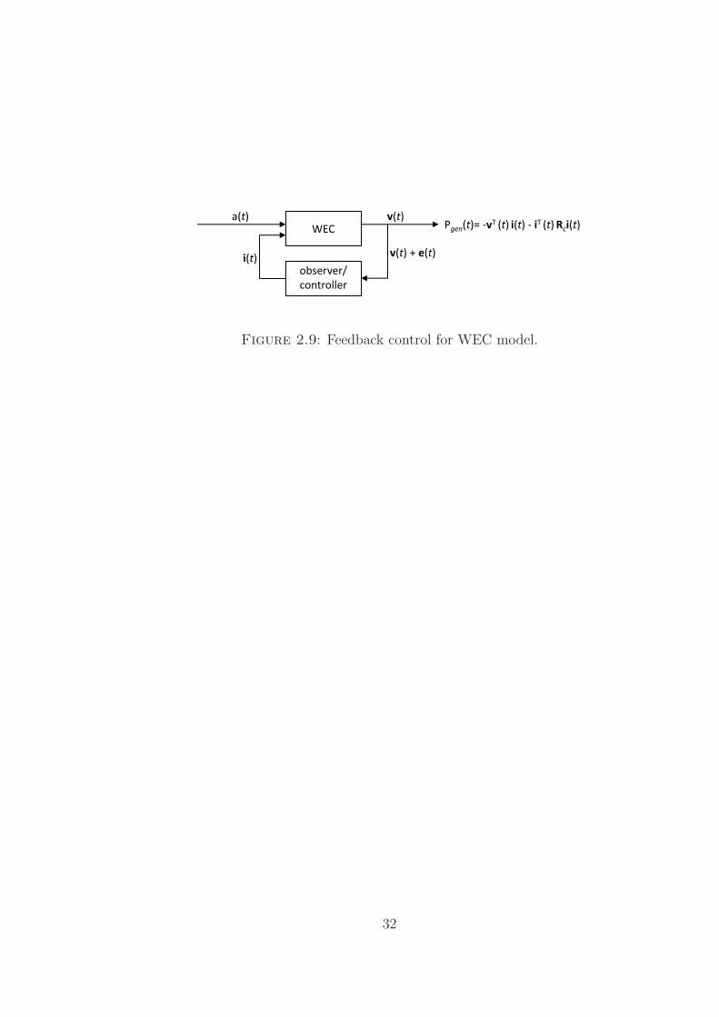
Figure 2.9: Feedback control for WEC model.
32
3
Optimal Noncausal Performance
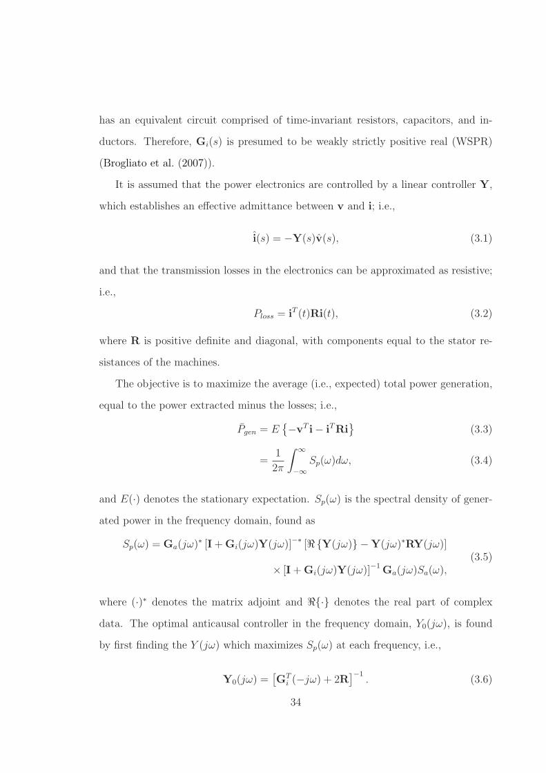
Knowing past, current, and future wave disturbances, it is possible to control a
WEC in a way that maximizes energy production using a linear controller. However,
since the future wave disturbance can be used to determine the optimal control law,
the control law is not necessarily causal. A control law that uses information about
future wave disturbances is impractical because this requires a way for buoys to sense
its surroundings and use some form of prediction algorithm. However, an optimal
noncausal controller and its performance is important to the analysis provided in
this thesis because the performance of optimal causal control laws can be compared
to it.
With the system model defined for the WEC buoy and a characterization for the
stochastic ocean wave environment, the optimum power generation can be deter-
mined through classical impedance matching. To begin, both Ga(s) and Gi(s) are
presumed to be strictly proper. If Ga(s) is strictly proper, then the harvester will
have a finite bandwidth. If Gi(s) is not strictly proper, then it may not approach
zero as s → j∞ (a property of all physical systems) and that creates the potential
for an unrealistic controller. We will also assume that the transfer function Gi(s)
33
has an equivalent circuit comprised of time-invariant resistors, capacitors, and in-
ductors. Therefore, Gi(s) is presumed to be weakly strictly positive real (WSPR)
(Brogliato et al. (2007)).
It is assumed that the power electronics are controlled by a linear controller Y,
which establishes an effective admittance between v and i; i.e.,
i(s) = −Y(s)v(s), (3.1)
and that the transmission losses in the electronics can be approximated as resistive;
i.e.,
Ploss = iT (t)Ri(t), (3.2)
where R is positive definite and diagonal, with components equal to the stator re-
sistances of the machines.
The objective is to maximize the average (i.e., expected) total power generation,
equal to the power extracted minus the losses; i.e.,
Pgen = E
−vT i− iTRi
(3.3)
=1
2π
∫ ∞
−∞
Sp(ω)dω, (3.4)
and E(·) denotes the stationary expectation. Sp(ω) is the spectral density of gener-
ated power in the frequency domain, found as
Sp(ω) = Ga(jω)∗ [I+Gi(jω)Y(jω)]−∗ [ℜY(jω) −Y(jω)∗RY(jω)]
× [I+Gi(jω)Y(jω)]−1Ga(jω)Sa(ω),
(3.5)
where (·)∗ denotes the matrix adjoint and ℜ· denotes the real part of complex
data. The optimal anticausal controller in the frequency domain, Y0(jω), is found
by first finding the Y (jω) which maximizes Sp(ω) at each frequency, i.e.,
Y0(jω) =[
GTi (−jω) + 2R
]−1. (3.6)
34
0 0.5 1 1.5 2 2.510
−1
100
101
102
103
104
105
106
107
ω (rad/s)
Sp
(W-s
)
Ce = 2.5 × 10⁵ kg/s
Ce = 2.5 × 10⁴ kg/s
Ce = 2.5 × 10² kg/s
Figure 3.1: Anticausal harvester power spectra: T1 = 12 s. H1/3 = 1 m, γ = 1.
The Laplace-domain representation of Y0(s) is just the analytic continuation of the
controller above (MacMartin et al. (1991)).
Note that at no point in the determination of the optimal anticausal controller, is
it necessary to know Sa(ω). Rather, information about the sea state is only necessary
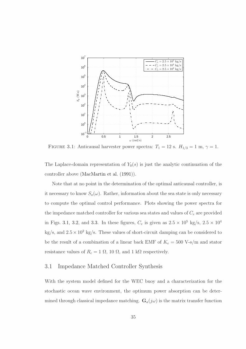
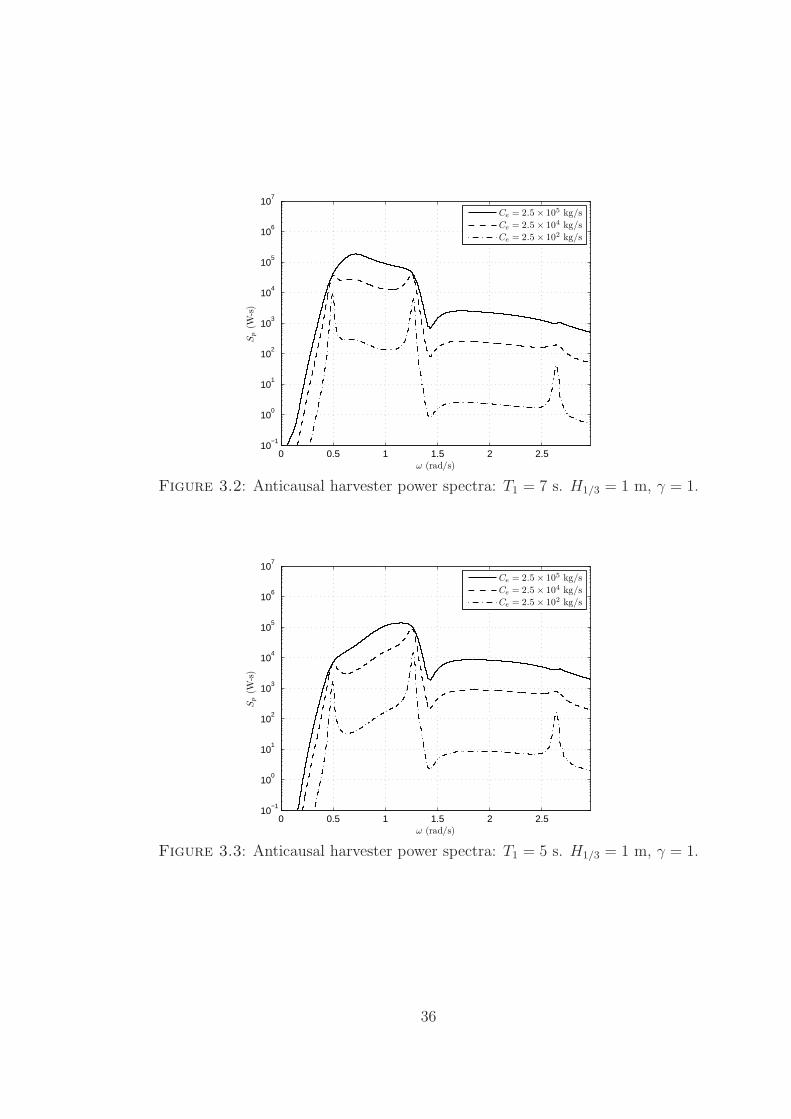
to compute the optimal control performance. Plots showing the power spectra for
the impedance matched controller for various sea states and values of Ce are provided
in Figs. 3.1, 3.2, and 3.3. In these figures, Ce is given as 2.5 × 10⁵ kg/s, 2.5 × 10⁴
kg/s, and 2.5× 10² kg/s. These values of short-circuit damping can be considered to
be the result of a combination of a linear back EMF of Ke = 500 V-s/m and stator
resistance values of Rc = 1 Ω, 10 Ω, and 1 kΩ respectively.
3.1 Impedance Matched Controller Synthesis
With the system model defined for the WEC buoy and a characterization for the
stochastic ocean wave environment, the optimum power absorption can be deter-
mined through classical impedance matching. Ga(jω) is the matrix transfer function
35
0 0.5 1 1.5 2 2.510
−1
100
101
102
103
104
105
106
107
ω (rad/s)
Sp
(W-s
)
Ce = 2.5 × 10⁵ kg/s
Ce = 2.5 × 10⁴ kg/s
Ce = 2.5 × 10² kg/s
Figure 3.2: Anticausal harvester power spectra: T1 = 7 s. H1/3 = 1 m, γ = 1.
0 0.5 1 1.5 2 2.510
−1
100
101
102
103
104
105
106
107
ω (rad/s)
Sp
(W-s
)
Ce = 2.5 × 10⁵ kg/s
Ce = 2.5 × 10⁴ kg/s
Ce = 2.5 × 10² kg/s
Figure 3.3: Anticausal harvester power spectra: T1 = 5 s. H1/3 = 1 m, γ = 1.
36
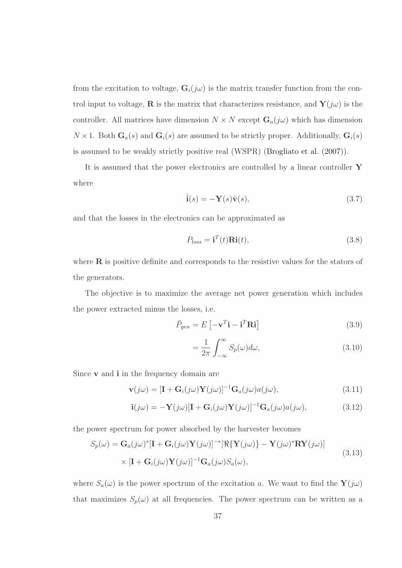
from the excitation to voltage, Gi(jω) is the matrix transfer function from the con-
trol input to voltage, R is the matrix that characterizes resistance, and Y(jω) is the
controller. All matrices have dimension N ×N except Ga(jω) which has dimension
N ×1. Both Ga(s) and Gi(s) are assumed to be strictly proper. Additionally, Gi(s)
is assumed to be weakly strictly positive real (WSPR) (Brogliato et al. (2007)).
It is assumed that the power electronics are controlled by a linear controller Y
where
i(s) = −Y(s)v(s), (3.7)
and that the losses in the electronics can be approximated as
Ploss = iT (t)Ri(t), (3.8)
where R is positive definite and corresponds to the resistive values for the stators of
the generators.
The objective is to maximize the average net power generation which includes
the power extracted minus the losses, i.e.
Pgen = E[
−vT i− iTRi]
(3.9)
=1
2π
∫ ∞
−∞
Sp(ω)dω, (3.10)
Since v and i in the frequency domain are
v(jω) = [I+Gi(jω)Y(jω)]−1Ga(jω)a(jω), (3.11)
i(jω) = −Y(jω)[I+Gi(jω)Y(jω)]−1Ga(jω)a(jω), (3.12)
the power spectrum for power absorbed by the harvester becomes
Sp(ω) = Ga(jω)∗[I+Gi(jω)Y(jω)]−∗[ℜY(jω) −Y(jω)∗RY(jω)]
× [I+Gi(jω)Y(jω)]−1Ga(jω)Sa(ω),(3.13)
where Sa(ω) is the power spectrum of the excitation a. We want to find the Y(jω)
that maximizes Sp(ω) at all frequencies. The power spectrum can be written as a
37
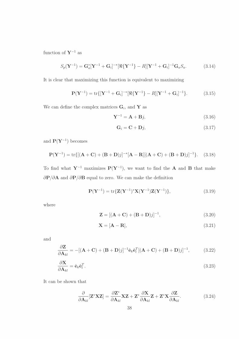
function of Y−1 as
Sp(Y−1) = G∗
a[Y−1 +Gi]
−∗[ℜY−1 −R][Y−1 +Gi]−1GaSa. (3.14)
It is clear that maximizing this function is equivalent to maximizing
P(Y−1) = tr[Y−1 +Gi]−∗[ℜY−1 −R][Y−1 +Gi]
−1. (3.15)
We can define the complex matrices Gi, and Y as
Y−1 = A+Bj, (3.16)
Gi = C+Dj, (3.17)
and P(Y−1) becomes
P(Y−1) = tr[(A+C) + (B+D)j]−∗[A−R][(A+C) + (B+D)j]−1. (3.18)
To find what Y−1 maximizes P(Y−1), we want to find the A and B that make
∂P/∂A and ∂P/∂B equal to zero. We can make the definition
P(Y−1) = trZ(Y−1)∗X(Y−1)Z(Y−1), (3.19)
where
Z = [(A+C) + (B+D)j]−1, (3.20)
X = [A−R], (3.21)
and
∂Z
∂Akl
= −[(A+C) + (B+D)j]−1ekeTl [(A+C) + (B+D)j]−1, (3.22)
∂X
∂Akl
= ekeTl . (3.23)
It can be shown that
∂
∂Akl
[Z∗XZ] =∂Z∗
∂Akl
XZ+ Z∗ ∂X
∂Akl
Z+ Z∗X∂Z
∂Akl
. (3.24)
38
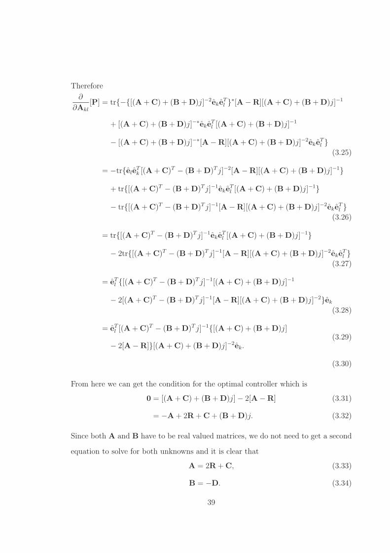
Therefore
∂
∂Akl
[P] = tr−[(A+C) + (B+D)j]−2ekeTl ∗[A−R][(A+C) + (B+D)j]−1
+ [(A+C) + (B+D)j]−∗ekeTl [(A+C) + (B+D)j]−1
− [(A+C) + (B+D)j]−∗[A−R][(A+C) + (B+D)j]−2ekeTl
(3.25)
= −treleTk [(A+C)T − (B+D)T j]−2[A−R][(A+C) + (B+D)j]−1
+ tr[(A+C)T − (B+D)T j]−1ekeTl [(A+C) + (B+D)j]−1
− tr[(A+C)T − (B+D)T j]−1[A−R][(A+C) + (B+D)j]−2ekeTl
(3.26)
= tr[(A+C)T − (B+D)T j]−1ekeTl [(A+C) + (B+D)j]−1
− 2tr[(A+C)T − (B+D)T j]−1[A−R][(A+C) + (B+D)j]−2ekeTl
(3.27)
= eTl [(A+C)T − (B+D)T j]−1[(A+C) + (B+D)j]−1
− 2[(A+C)T − (B+D)T j]−1[A−R][(A+C) + (B+D)j]−2ek(3.28)
= eTl [(A+C)T − (B+D)T j]−1[(A+C) + (B+D)j]
− 2[A−R][(A+C) + (B+D)j]−2ek.(3.29)
(3.30)
From here we can get the condition for the optimal controller which is
0 = [(A+C) + (B+D)j]− 2[A−R] (3.31)
= −A+ 2R+C+ (B+D)j. (3.32)
Since both A and B have to be real valued matrices, we do not need to get a second
equation to solve for both unknowns and it is clear that
A = 2R+C, (3.33)
B = −D. (3.34)
39
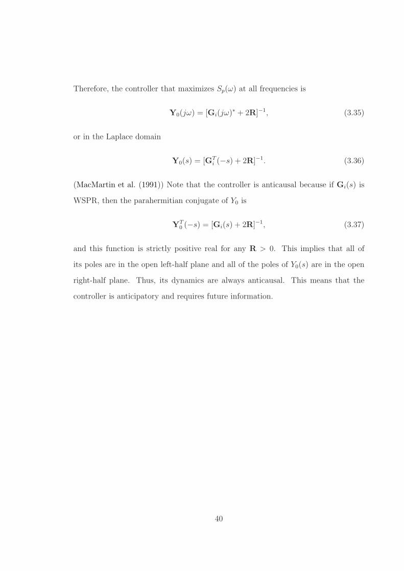
Therefore, the controller that maximizes Sp(ω) at all frequencies is
Y0(jω) = [Gi(jω)∗ + 2R]−1, (3.35)
or in the Laplace domain
Y0(s) = [GTi (−s) + 2R]−1. (3.36)
(MacMartin et al. (1991)) Note that the controller is anticausal because if Gi(s) is
WSPR, then the parahermitian conjugate of Y0 is
YT0 (−s) = [Gi(s) + 2R]−1, (3.37)
and this function is strictly positive real for any R > 0. This implies that all of
its poles are in the open left-half plane and all of the poles of Y0(s) are in the open
right-half plane. Thus, its dynamics are always anticausal. This means that the
controller is anticipatory and requires future information.
40
4
Finite-Dimensional Approximation
In order to determine the optimal causal performance it is necessary to have finite-
dimensional state space models that characterize the transfer functions Ga and Gi.
It is also necessary to have a finite-dimensional state space model that describes
the wave height process, i.e. a filter that has an equivalent power spectrum to the
desired JONSWAP power spectrum that is subjected to white noise of unit spectral
intensity. It should be noted that these finite-dimensional state space models will be
inexact because the hydrodynamic functions Fa(ω), Mc(ω), and Cc(ω) from Ch. 2
are infinite-dimensional and the JONSWAP power spectrum is characterized by a
piecewise function that is not rational.
The approximated state spaces forGa andGi were found using the subspace tech-
niques originally proposed in McKelvey et al. (1996) for determining finite-dimensional
approximations for infinite-dimensional systems characterized by frequency response
data. Although this algorithm does not give optimal estimates of a given order, it
does identify the balanced truncations of infinite dimensional systems in discrete-
time from frequency-domain data. The approximated state space corresponding to
the JONSWAP spectrum was found using a simple iterative non-linear search algo-
41
rithm.
4.1 JONSWAP power spectrum approximation
Finding a finite-dimensional transfer function with a power spectrum that is close to
the JONSWAP spectrum can be done by minimizing the sum of the squared-error
between the actual JONSWAP spectrum and the absolute value of the candidate
continuous-time transfer function squared,
ǫ =M∑
i=1
(
‖HJ(i)‖2 − Sa(i))2
(4.1)
whereM is the number of samples in the sampled version (M samples linearly spaced
on ω ∈ [0, ωf ]) of Sa and the candidate transfer function which is of the form
HJ(s) =b1s
N−1 + b2sN + . . .+ bN−1s
a1sN + a2sN−1 + . . .+ aN+1
, (4.2)
N is the model order, and ωf is a frequency value where Sa has converged to near
zero. The poles of the system are constrained to be in the left-half-plane in order
to ensure stability. This is done by flipping any unstable poles across the imaginary
axis and this does not affect the fit since the it does not affect the magnitude of the
transfer function. Note that the DC gain of the transfer function is zero. Without
this property, large errors can be seen at low frequencies during the later analysis
since it could appear that there is a nontrivial amount of power at those frequencies.
The minimization was accomplished through the use of a simplex algorithm. The
transfer function can be converted to a continuous-time state space realization that
has the form
xJ = AJxJ +BJw, (4.3)
a = CJxJ , (4.4)
42
where w(t) is a scalar white noise process with spectral intensity equal to 1. The
techniques described above are similar to what is done in Spanos (1986). In this
analysis, it was found that a state space of order 4 was sufficient to render close
matching to JONSWAP spectra for reasonable sharpness factors. Some examples of
JONSWAP power spectra and their finite-dimensional approximations are shown in
Fig. 4.1. It was also observed thatM = 1000 and ωf = 6 rad/s were sufficient values.
4.2 State-space model identification from frequency domain data
Given the frequency domain data for the infinite dimensional transfer functions Ga
and Gi it is possible to find their corresponding approximate finite-dimensional state
space models. The first step to the identification algorithm is to expand uniformly
spaced experimental frequency-response data of the single-input-single-ouput (SISO)
system, or SISO subsystem of a larger system, being considered according to
G(e−jθ) = G∗(ejθ), 0 ≤ θ ≤ π, (4.5)
where θ is the discrete-time frequency as
GM+k ≡ G∗M−k, k = 1, . . . ,M − 1, (4.6)
and perform the 2M -point inverse discrete-time Fourier transform (DFT) on the
expanded data
gi ≡1
2M
2M−1∑
k=0
Gkej2πik/2M , i = 0, . . . , q + r − 1, (4.7)
to determine the estimates of the impulse-response coefficients of gi.
The next step is to construct the q × r-block Hankel matrix
Hqr ≡
g1 · · · gr...
. . ....
gq · · · gq+r−1
, (4.8)
43
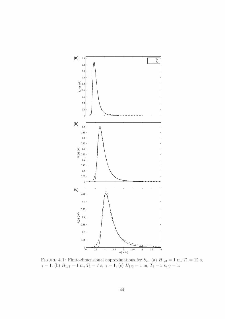
Figure 4.1: Finite-dimensional approximations for Sa. (a) H1/3 = 1 m, T1 = 12 s,γ = 1; (b) H1/3 = 1 m, T1 = 7 s, γ = 1; (c) H1/3 = 1 m, T1 = 5 s, γ = 1.
44
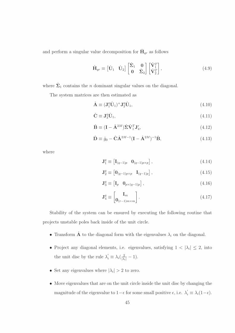
and perform a singular value decomposition for Hqr as follows
Hqr ≡[
U1 U2
]
[
Σ1 0
0 Σ2
] [
VT1
VT2
]
, (4.9)
where Σ1 contains the n dominant singular values on the diagonal.
The system matrices are then estimated as
A ≡ (Jq1U1)
+Jq2U1, (4.10)
C ≡ Jq3U1, (4.11)
B ≡ (I− A2M)ΣVT1 J
r4, (4.12)
D ≡ g0 − CA2M−1(I− A2M)−1B, (4.13)
where
Jq1 ≡
[
I(q−1)p 0(q−1)p×p
]
, (4.14)
Jq2 ≡
[
0(q−1)p×p I(q−1)p
]
, (4.15)
Jq3 ≡
[
Ip 0p×(q−1)p
]
, (4.16)
Jq4 ≡
[
Im0(r−1)m×m
]
. (4.17)
Stability of the system can be ensured by executing the following routine that
projects unstable poles back inside of the unit circle.
• Transform A to the diagonal form with the eigenvalues λi on the diagonal.
• Project any diagonal elements, i.e. eigenvalues, satisfying 1 < |λi| ≤ 2, into
the unit disc by the rule λ′
i ≡ λi(2
|λi|− 1).
• Set any eigenvalues where |λi| > 2 to zero.
• Move eigenvalues that are on the unit circle inside the unit disc by changing the
magnitude of the eigenvalue to 1−ǫ for some small positive ǫ, i.e. λ′
i ≡ λi(1−ǫ).
45
• Transform A back to its original form.
• Go on to determine B and D as in (4.12) and (4.13).
A model order of 12 was found to be sufficient for each component of Ga and a
model order of 6 was found to be sufficient for each component of Gi. A model order
was considered sufficient if it managed to capture all of the details of the magnitude
and phase data of a subsystem.
4.3 Augmented state-spaces
The algorithm presented in the previous section was run on each SISO component
in the discrete-time form of the matrix transfer functions Ga and Gi and the corre-
sponding state-space models were converted from discrete-time to continuous-time
models using a standard bilinear approximation. The individual state spaces could
then be augmented together to create finite-dimensional state spaces of the form
Ga ∼[
Aa Ba
Ca 0
]
(4.18)
Gi ∼[
Ai Bi
Ci 0
]
. (4.19)
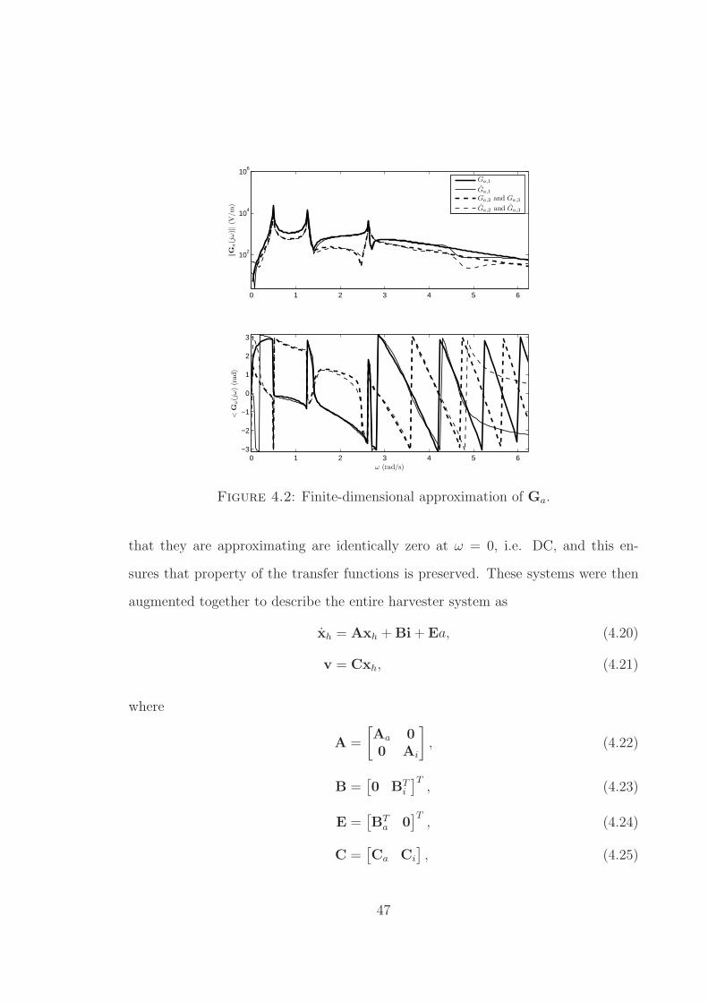
Figs. 4.2 and 4.3 show the frequency domain data for Ga and Gi and their finite-
dimensional approximations. The quality of the fits are typical and in this case the
model order for each component of Ga and Gi are 12 and 6 respectively. The fits
also reflect a final balanced reduction augmented system shown above where the
final model order of the finite-dimensional approximations for Ga and Gi are 19 and
10 respectively. Note that the plots are in log scale and thus what appear to be
large visible errors around low magnitude data are actually relatively unimportant.
Additionally, errors in phase around areas with low magnitude are unimportant.
It should be noted that although they are identified, the feedthrough terms are
neglected. They are left out because they are very small and the transfer functions
46
0 1 2 3 4 5 6
102
104
106
‖G
a(j
ω)‖
(V/m
)
0 1 2 3 4 5 6−3
−2
−1
0
1
2
3
<G
a(j
ω)
(rad)
ω (rad/s)
Ga,1
Ga,1
Ga,2 and Ga,3
Ga,2 and Ga,3
Figure 4.2: Finite-dimensional approximation of Ga.
that they are approximating are identically zero at ω = 0, i.e. DC, and this en-
sures that property of the transfer functions is preserved. These systems were then
augmented together to describe the entire harvester system as
xh = Axh +Bi+ Ea, (4.20)
v = Cxh, (4.21)
where
A =
[
Aa 0
0 Ai
]
, (4.22)
B =[
0 BTi
]T, (4.23)
E =[
BTa 0
]T, (4.24)
C =[
Ca Ci
]
, (4.25)
47
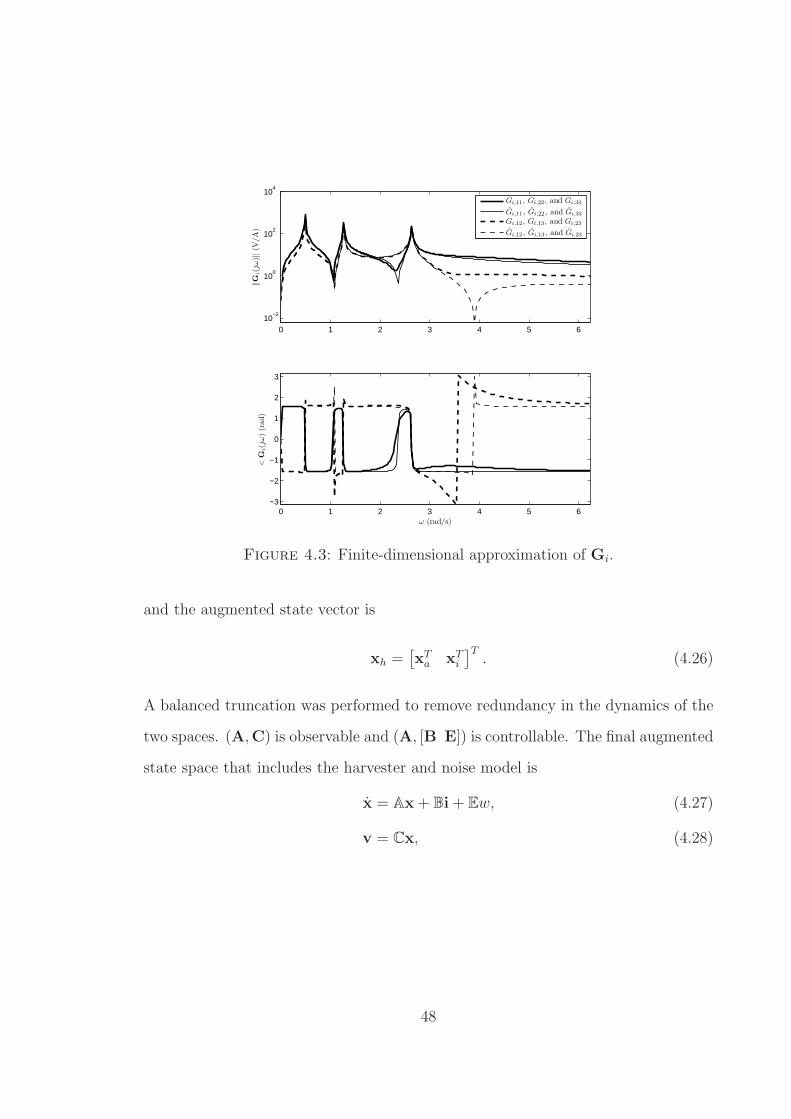
0 1 2 3 4 5 610
−2
100
102
104
‖G
i(j
ω)‖
(V/A
)
0 1 2 3 4 5 6−3
−2
−1
0
1
2
3
<G
i(j
ω)
(rad)
ω (rad/s)
Gi,11, Gi,22, and Gi,33
Gi,11 , Gi,22 , and Gi,33
Gi,12, Gi,13, and Gi,23
Gi,12 , Gi,13 , and Gi,23
Figure 4.3: Finite-dimensional approximation of Gi.
and the augmented state vector is
xh =[
xTa xT
i
]T. (4.26)
A balanced truncation was performed to remove redundancy in the dynamics of the
two spaces. (A,C) is observable and (A, [B E]) is controllable. The final augmented
state space that includes the harvester and noise model is
x = Ax+ Bi+ Ew, (4.27)
v = Cx, (4.28)
48
where the augmented matrices A, B, E, and C are
A =
[
A ECJ
0 AJ
]
, (4.29)
B =[
B 0]T, (4.30)
E =[
0 BJ
]T, (4.31)
C =[
C 0]
, (4.32)
and the augmented state vector is
x =[
xTh xT
J
]T. (4.33)
4.4 Additional identification techniques
In an attempt to find more accurately identified systems, a couple of techniques
were developed. The first such technique is to find the Ga that characterizes the
relationship between the wave amplitude, which is several meters in front of the buoy
in the direction of the oncoming waves, and the output voltage. This is important
because the hydrodynamic forces acting on the buoy are affected by waves that have
not yet passed by the buoy and is similar to instituting a time delay, but simpler
for this application. Wave amplitudes that are increasingly further away from the
buoy have a dimishing effect. It was found that the wave amplitude approximately
5 m out in front of the buoy provides enough spatial delay to accurately identify Ga
while not sacrificing too much in terms of the increased model order needed to model
such a delay.
The second technique is to add a static admittance to the system in order to
bring down the peaks of the transfer functions around the modes of resonance so
that the identification algorithm will be less likely to sacrifice accuracy over some
ranges of frequency that might ultimately prove to be important. This was intended
to overcome the shortcomings from previously explored identification routines such as
49

the one found in Bayard (1994) and the built-in routines in MATLAB, but ultimately,
it was not used since the identification routine in McKelvey et al. (1996) works very
well. Details for this technique are provided in Appendix A.
50
5
Optimal Causal Performance
Consider the augmented continuous-time finite dimensional state space for the WEC
given in (4.27) and (4.28) that includes the sea state as a filtered noise process within
it. Now it is possible to use H2 control theory to determine the optimal causal power
generation and the corresponding controller for both the full-state feedback case
and the more realistic output feedback case with measurement noise. It is much
more practical to have a causal controller that relies only on the current and past
output from the system, which are in the form of voltages measured at the generator
terminals, instead of a noncausal controller that relies on knowledge of future wave
disturbances.
51
5.1 Full-state feedback
The objective is to find the full-state feedback law K : x → i which maximizes Pgen,
or equivalently, which minimizes
−Pgen = E
vT i+ iTRi
(5.1)
=1
2E
[
xh
i
]T [0 CT
C 2R
] [
xh
i
]
. (5.2)
This constitutes an LQG optimal control problem, but is non-standard because the
performance functional is sign-indefinite. It is a standard result from Astrom (1970)
that the optimal control solution, if it exists, is
i = Kx = −12R−1[BTP+ C]x, (5.3)
where P is the stabilizing solution to the algebraic Riccati equation
0 = ATP+PA− 1
2[BTP+ C]TR−1[BTP+ C]. (5.4)
The expression for the optimal causal power spectrum with full-state feedback is
Sp(ω) = −ℜ [H∗i (jω)Hv(jω)]−H∗
i (jω)RHi(jω), (5.5)
where
Hi(jω) = K [jωI− A− BK]−1E, (5.6)
Hv(jω) = C [jωI− A− BK]−1E. (5.7)
and a closed-form expression for the optimal Pgen is
P optgen = −1
2E
TPE. (5.8)
Given a WSPR system, P optgen is always positive and the optimal controller is always
stabilizing (Scruggs (2010)).
52
5.2 Output feedback
In practice, the state vector x will need to be estimated from v. This can be done via
a Kalman-Bucy filter that keeps a running estimate of the system states according
to the differential equation
ddtx = Ax+ Bi+ F (Cx− v) , (5.9)
where x is the estimate of x. Assuming white noise in the measurement channels for
v, with spectral intensity matrix νI, the optimal estimates are thus obtained via the
standard Kalman gain; i.e.,
F = − 1νSCT , (5.10)
where S is the solution to the matrix Riccati equation
0 = AS+ SAT − 1νSCT
CS+ EET . (5.11)
With K defined in (5.3), the augmented closed-loop system becomes
xc = Acxc + Ecw, (5.12)
v = Ccxc, (5.13)
where
Ac =
[
A BK
−FC (A+ FC+ BK)
]
, (5.14)
Ec =
[
E
0
]
, (5.15)
Cc =[
C 0]
, (5.16)
and
xc =[
xT xT]T. (5.17)
Defining the augmented controller as
Kc =[
0 K]
, (5.18)
53
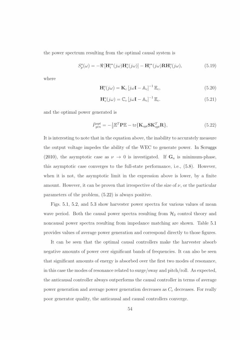
the power spectrum resulting from the optimal causal system is
Sop(ω) = −ℜ [Ho∗
i (jω)Hov(jω)]−Ho∗
i (jω)RHoi (jω), (5.19)
where
Hoi (jω) = Kc [jωI− Ac]
−1Ec, (5.20)
Hov(jω) = Cc [jωI− Ac]
−1Ec. (5.21)
and the optimal power generated is
P optgen = −1
2E
TPE− trKoptSKToptR, (5.22)
It is interesting to note that in the equation above, the inability to accurately measure
the output voltage impedes the ability of the WEC to generate power. In Scruggs
(2010), the asymptotic case as ν → 0 is investigated. If Ga is minimum-phase,
this asymptotic case converges to the full-state performance, i.e., (5.8). However,
when it is not, the asymptotic limit in the expression above is lower, by a finite
amount. However, it can be proven that irrespective of the size of ν, or the particular
parameters of the problem, (5.22) is always positive.
Figs. 5.1, 5.2, and 5.3 show harvester power spectra for various values of mean
wave period. Both the causal power spectra resulting from H2 control theory and
noncausal power spectra resulting from impedance matching are shown. Table 5.1
provides values of average power generation and correspond directly to those figures.
It can be seen that the optimal causal controllers make the harvester absorb
negative amounts of power over significant bands of frequencies. It can also be seen
that significant amounts of energy is absorbed over the first two modes of resonance,
in this case the modes of resonance related to surge/sway and pitch/roll. As expected,
the anticausal controller always outperforms the causal controller in terms of average
power generation and average power generation decreases as Ce decreases. For really
poor generator quality, the anticausal and causal controllers converge.
54
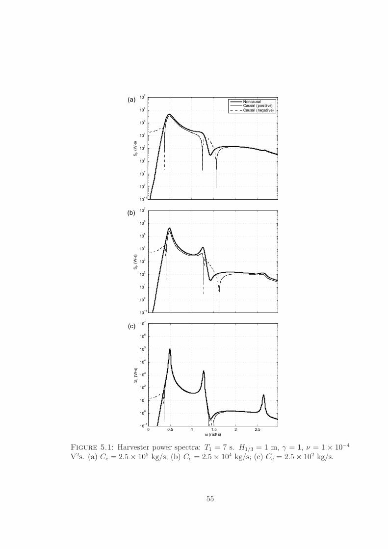
Figure 5.1: Harvester power spectra: T1 = 7 s. H1/3 = 1 m, γ = 1, ν = 1 × 10⁻⁴
V2s. (a) Ce = 2.5× 10⁵ kg/s; (b) Ce = 2.5× 10⁴ kg/s; (c) Ce = 2.5× 10² kg/s.
55
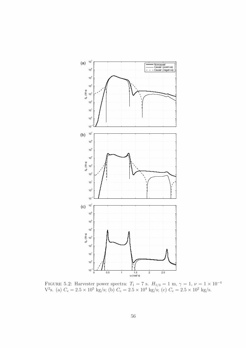
Figure 5.2: Harvester power spectra: T1 = 7 s. H1/3 = 1 m, γ = 1, ν = 1 × 10⁻⁴
V2s. (a) Ce = 2.5× 10⁵ kg/s; (b) Ce = 2.5× 10⁴ kg/s; (c) Ce = 2.5× 10² kg/s.
56
Figure 5.3: Harvester power spectra: T1 = 5 s. H1/3 = 1 m, γ = 1, ν = 1 × 10⁻⁴
V2s. (a) Ce = 2.5× 10⁵ kg/s; (b) Ce = 2.5× 10⁴ kg/s; (c) Ce = 2.5× 10² kg/s.
57
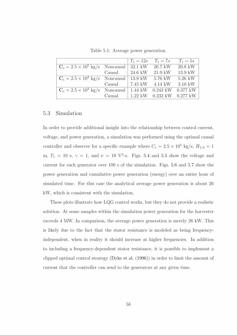
Table 5.1: Average power generation.
T1 = 12s T1 = 7s T1 = 5sCe = 2.5× 10⁵ kg/s Noncausal 32.1 kW 26.7 kW 20.8 kW
Causal 24.6 kW 21.9 kW 13.9 kWCe = 2.5× 10⁴ kg/s Noncausal 13.8 kW 5.76 kW 5.26 kW
Causal 7.45 kW 4.14 kW 3.10 kWCe = 2.5× 10² kg/s Noncausal 1.44 kW 0.243 kW 0.377 kW
Causal 1.22 kW 0.232 kW 0.277 kW
5.3 Simulation
In order to provide additional insight into the relationship between control current,
voltage, and power generation, a simulation was performed using the optimal causal
controller and observer for a specific example where Ce = 2.5 × 10⁵ kg/s, H1/3 = 1
m, T1 = 10 s, γ = 1, and ν = 10 V2-s. Figs. 5.4 and 5.5 show the voltage and
current for each generator over 100 s of the simulation. Figs. 5.6 and 5.7 show the
power generation and cumulative power generation (energy) over an entire hour of
simulated time. For this case the analytical average power generation is about 26
kW, which is consistent with the simulation.
These plots illustrate how LQG control works, but they do not provide a realistic
solution. At some samples within the simulation power generation for the harvester
exceeds 4 MW. In comparison, the average power generation is merely 26 kW. This
is likely due to the fact that the stator resistance is modeled as being frequency-
independent, when in reality it should increase at higher frequencies. In addition
to including a frequency-dependent stator resistance, it is possible to implement a
clipped optimal control strategy (Dyke et al. (1996)) in order to limit the amount of
current that the controller can send to the generators at any given time.
58
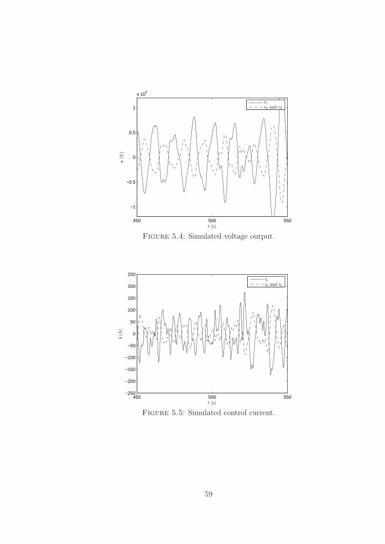
450 500 550
−1
−0.5
0
0.5
1
x 104
t (s)
v(V
)
v1
v2 and v3
Figure 5.4: Simulated voltage output.
450 500 550−250
−200
−150
−100
−50
0
50
100
150
200
250
t (s)
i(A
)
i1i2 and i3
Figure 5.5: Simulated control current.
59
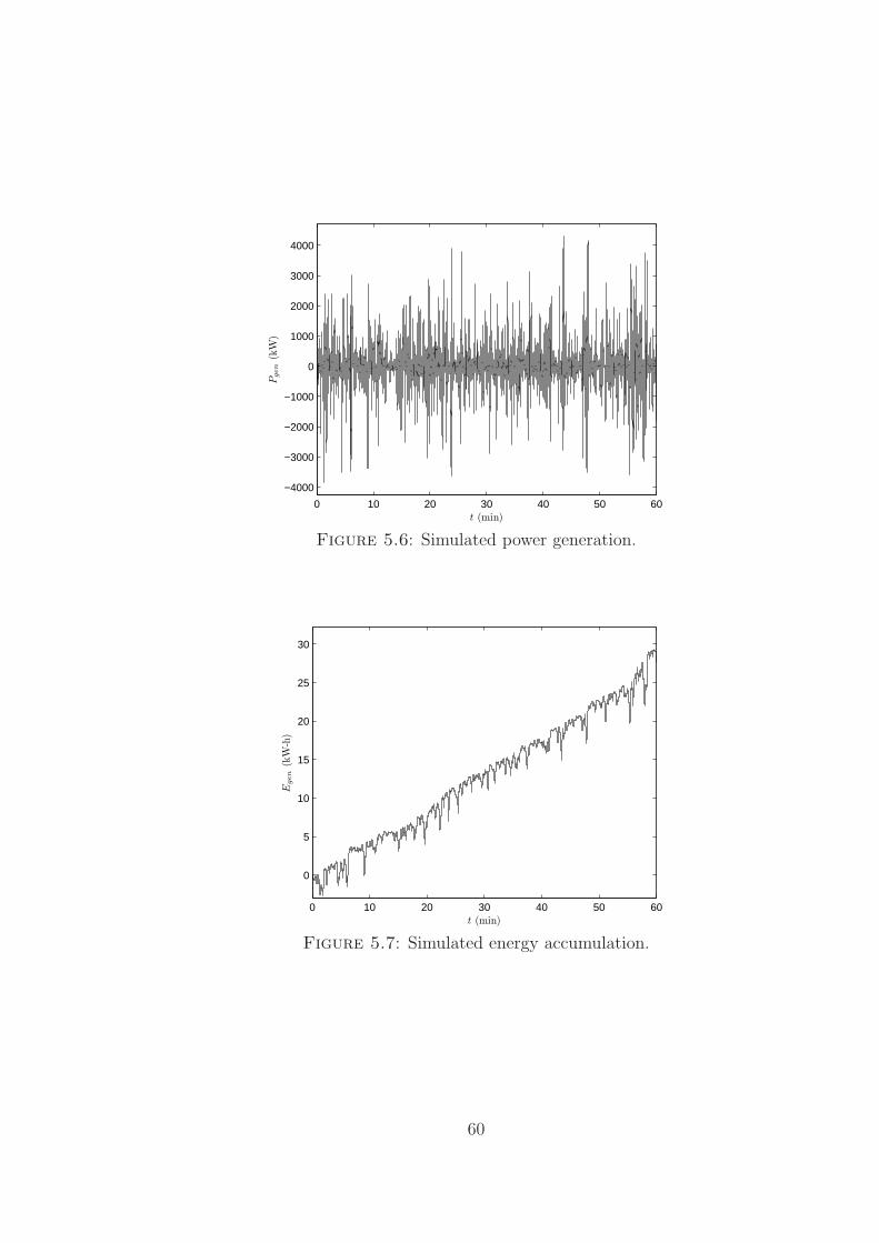
0 10 20 30 40 50 60
−4000
−3000
−2000
−1000
0
1000
2000
3000
4000
t (min)
Pgen
(kW
)
Figure 5.6: Simulated power generation.
0 10 20 30 40 50 60
0
5
10
15
20
25
30
t (min)
Egen
(kW
-h)
Figure 5.7: Simulated energy accumulation.
60
6
Adaptive Control
The causal controller described in the previous chapter assumes that the character-
istics of the sea state (i.e., γ, T1, and H1/3), along with the harvester dynamics are
known. However, in practice the sea state slowly varies over time and the WEC
needs a way to adapt in order to retain near optimal performance. This can be
accomplished either by remotely observing the sea state and having the controller
changed accordingly, or automatically by including a real-time system identification
algorithm to implement a self-tuning adaptive controller.
6.1 Adaptive control performance
If the controller is not made to adapt to changes in sea state, these changes will
result in sub-optimal performance. Considering only voltage feedback, the average
power generation is
Pgen = E−vT i− iTRi, (6.1)
= E−xTc C
Tc Kcxc − xT
c KTc RKcxc, (6.2)
= −trCTc KcΦ +KT
c RKcΦ, (6.3)
61
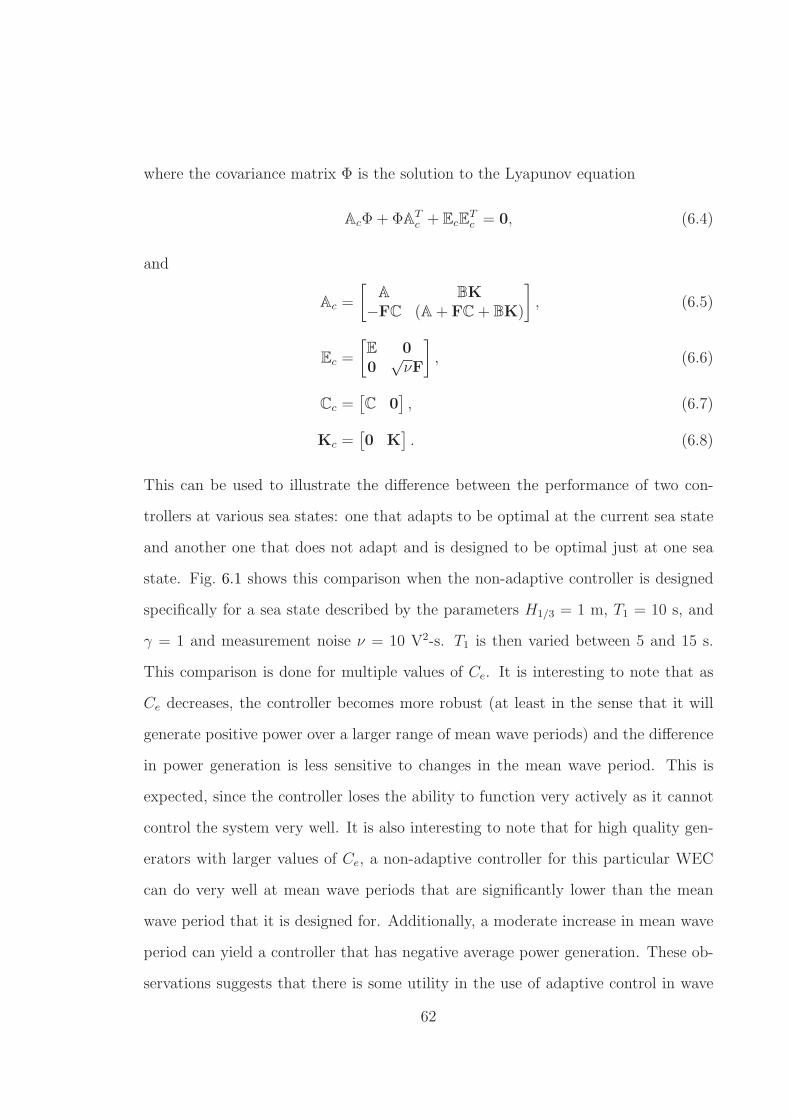
where the covariance matrix Φ is the solution to the Lyapunov equation
AcΦ + ΦATc + EcE
Tc = 0, (6.4)
and
Ac =
[
A BK
−FC (A+ FC+ BK)
]
, (6.5)
Ec =
[
E 0
0√νF
]
, (6.6)
Cc =[
C 0]
, (6.7)
Kc =[
0 K]
. (6.8)
This can be used to illustrate the difference between the performance of two con-
trollers at various sea states: one that adapts to be optimal at the current sea state
and another one that does not adapt and is designed to be optimal just at one sea
state. Fig. 6.1 shows this comparison when the non-adaptive controller is designed
specifically for a sea state described by the parameters H1/3 = 1 m, T1 = 10 s, and
γ = 1 and measurement noise ν = 10 V2-s. T1 is then varied between 5 and 15 s.
This comparison is done for multiple values of Ce. It is interesting to note that as
Ce decreases, the controller becomes more robust (at least in the sense that it will
generate positive power over a larger range of mean wave periods) and the difference
in power generation is less sensitive to changes in the mean wave period. This is
expected, since the controller loses the ability to function very actively as it cannot
control the system very well. It is also interesting to note that for high quality gen-
erators with larger values of Ce, a non-adaptive controller for this particular WEC
can do very well at mean wave periods that are significantly lower than the mean
wave period that it is designed for. Additionally, a moderate increase in mean wave
period can yield a controller that has negative average power generation. These ob-
servations suggests that there is some utility in the use of adaptive control in wave
62
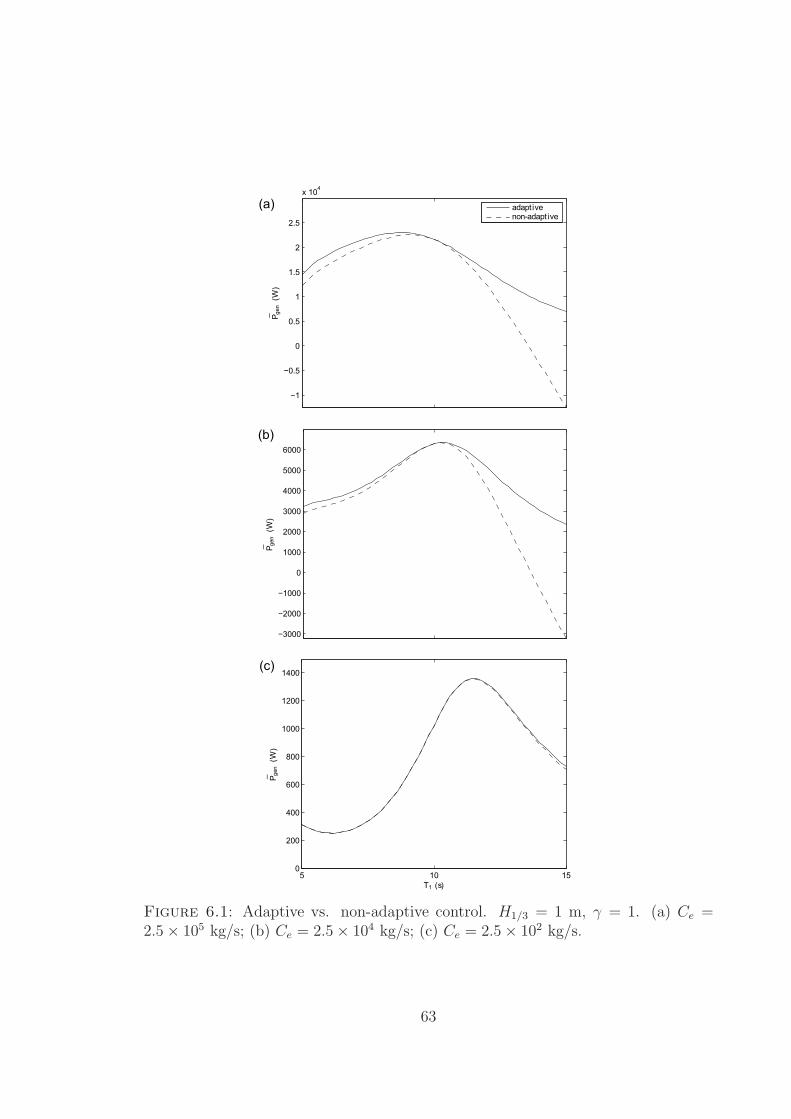
Figure 6.1: Adaptive vs. non-adaptive control. H1/3 = 1 m, γ = 1. (a) Ce =2.5× 10⁵ kg/s; (b) Ce = 2.5× 10⁴ kg/s; (c) Ce = 2.5× 10² kg/s.
63
Figure 6.2: Conceptual diagram of an indirect STR for a WEC
energy conversion.
6.2 Future work
The need for an adaptive control algorithm has been demonstrated in the previous
section by comparing the performance of a controller that knows the sea state ex-
actly and is designed accordingly and one that is designed for a single sea state.
There are many adaptive control algorithms that can be applied to this problem.
One such control algorithm is known as an indirect self-tuning regulator (STR) and
is shown in Fig. 6.2. An indirect STR involves a recursive estimation of the sys-
tem and subsequent controller and observer gain design as if the system estimate
is the same as the true system. This is known as the certainty equivalence prin-
ciple. It is proposed that such a recursive estimation can be accomplished by the
use of the recursive extended least-squares (RELS) algorithm. Information on STRs
(and other adaptive control algorithms) and the RELS algorithm can be found in
Astrom and Wittenmark (1995).
64
6.2.1 Recursive extended least-squares
Some systems, such as the augmented system for the WEC in this thesis, have a
non-deterministic input in addition to deterministic ones. In the case of the WEC,
the wave height, which is a fixed distance in front of the buoy, is non-deterministic
while the control current sent to the generators is deterministic. These systems
require a way of treating the non-deterministic input as filtered white noise, if that
is a reasonable way to model such an input. This can be done using the RELS
algorithm.
A RELS algorithm is given in Astrom and Wittenmark (1995) for a system with
one deterministic input, one non-deterministic filtered white noise input, and one
output. This can be expanded into a system with an arbitrary amount of all three.
Consider a system of order n with N deterministic inputs and M outputs. The
relationship between the ith output yi, all of the inputs u1, . . . , uN, and the ith (or
only) white noise disturbance ei is
Ai(q)yi(t) =N∑
j=1
Bij(q)uj(t) +Ci(q)ei(t), (6.9)
where Ai(q), Bij(q), and Ci(q) are polynomials in the forward shift operator q, i.e.
Ai(q)yi(t) = yi(t) + ai1yi(t− 1) + . . .+ ainy(t− n), (6.10)
Bij(q)uj(t) = bij1uj(t− 1) + bij2uj(t− 2) + . . .+ bijnuj(t− n), (6.11)
Ci(q)ei(t) = ci1ei(t− 1) + ci2ei(t− 2) + . . .+ cinei(t− n), (6.12)
and ei(t) is white noise. The parameters of the polynomial Ci describe the corre-
lation of the disturbance for the output yi. Note that in this case, the polynomials
B(q) and C(q) are of order n− 1 while A(q) is order n. However, in a more general
formulation, all three may be of different order.
65
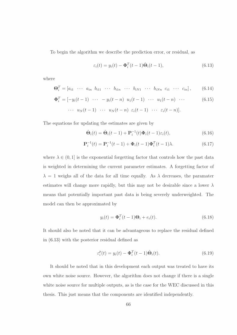
To begin the algorithm we describe the prediction error, or residual, as
εi(t) = yi(t)−ΦTi (t− 1)Θi(t− 1), (6.13)
where
ΘTi = [ai1 · · · ain bi11 · · · bi1n · · · biN1 · · · biNn ci1 · · · cin] , (6.14)
ΦTi = [−yi(t− 1) · · · − yi(t− n) u1(t− 1) · · · u1(t− n) · · · (6.15)
· · · uN(t− 1) · · · uN(t− n) εi(t− 1) · · · εi(t− n)].
The equations for updating the estimates are given by
Θi(t) = Θi(t− 1) +P−1i (t)Φi(t− 1)εi(t), (6.16)
P−1i (t) = P−1
i (t− 1) +Φi(t− 1)ΦTi (t− 1)λ. (6.17)
where λ ∈ (0, 1] is the exponential forgetting factor that controls how the past data
is weighted in determining the current parameter estimates. A forgetting factor of
λ = 1 weighs all of the data for all time equally. As λ decreases, the paramater
estimates will change more rapidly, but this may not be desirable since a lower λ
means that potentially important past data is being severely underweighted. The
model can then be approximated by
yi(t) = ΦTi (t− 1)Θi + ei(t). (6.18)
It should also be noted that it can be advantageous to replace the residual defined
in (6.13) with the posterior residual defined as
εpi (t) = yi(t)−ΦTi (t− 1)Θi(t). (6.19)
It should be noted that in this development each output was treated to have its
own white noise source. However, the algorithm does not change if there is a single
white noise source for multiple outputs, as is the case for the WEC discussed in this
thesis. This just means that the components are identified independently.
66
The model above can be converted directly into a discrete-time matrix transfer
function and subsequently changed into other forms such as discrete or continuous-
time state space models.
The RELS algorithm allows for the entire system estimate to be updated at each
sampling period, but it is not recommended that the controller and observer gain be
redesigned at each sampling period. This would require a high level of computation
as the discrete-time system estimate needs a lot of processing prior to being used in
the methods described in this theory. Even then, matrix Riccati equations must be
solved. It is recommended that the controller and observer gains are redesigned only
periodically, either at a set amount of time, or triggered by changes in performance
or system estimate that exceed some threshold. Also, the subsystem Gi may not
need to be recursively identified if it is assumed that it is time-invariant. This is a
fair assumption unless the WEC is designed to adapt its configuration in addition to
its control and observer gains.
There are additional problems that can arise through the use of an indirect STR
in conjunction with an RELS algorithm. These include the use of sufficiently large
model orders for the system estimates, and also the avoidance of overparameteriza-
tion. Additionally, simultaneous estimation and control may pose problems as it is
possible that a control input can create an output that makes it hard to observe the
effects of ocean waves. It may prove to be more practical to only recursively identify
the system when while the control input is turned off over relatively short periods of
time.
67
7
Conclusions
This thesis demonstrated how a WEC can be modeled as a finite-dimensional linear
state space model and how that model can then be used to determine the optimal
causal linear feedback control strategy for both the full-state feedback and voltage
feedback cases. Additionally, the voltage feedback case was compared to the optimal
noncausal control found through the use of classical impedance matching, which in a
realistic (i.e., stochastic) wave environment, results in an anticausal controller. Such
a controller is impractical, since it is anticipatory and requires information regarding
future wave excitiation to be known.
It has been shown that the determination of the optimal causal controller for
wave energy applications distills to a nonstandard H2 optimal control problem. This
problem can be solved provided that the hydrodynamic interaction model can be
approximated by a finite-dimensional state space. The example provided in the
thesis illustrates that constraining the controller to be causal modifies the power
flow for the WEC and generally results in frequency bands where average power
generation is negative, i.e., the controller is injecting power into the system. When
high quality machines are used, these bands can be quite significant.
68

Additionally, it was shown that the optimal controller is sensitive to changes in
the sea state, specifically the mean wave period. This is the most pronounced for
WECs with high quality generators. This provides motivation for the use of adaptive
control algorithms. An adaptive control algorithm known as an indirect self-tuning
regulator (STR) is proposed.
69
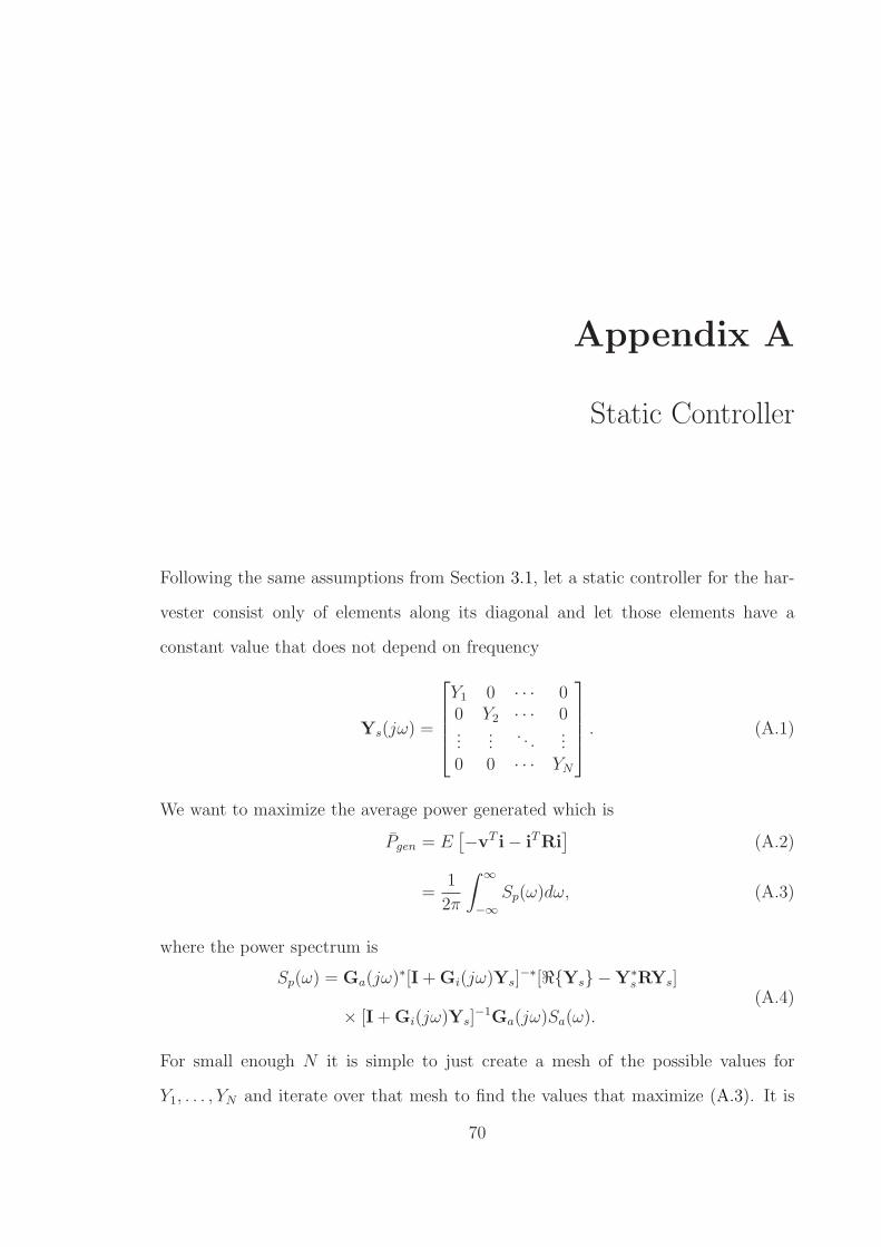
Appendix A
Static Controller
Following the same assumptions from Section 3.1, let a static controller for the har-
vester consist only of elements along its diagonal and let those elements have a
constant value that does not depend on frequency
Ys(jω) =
Y1 0 · · · 00 Y2 · · · 0...
.... . .
...0 0 · · · YN
. (A.1)
We want to maximize the average power generated which is
Pgen = E[
−vT i− iTRi]
(A.2)
=1
2π
∫ ∞
−∞
Sp(ω)dω, (A.3)
where the power spectrum is
Sp(ω) = Ga(jω)∗[I+Gi(jω)Ys]
−∗[ℜYs −Y∗sRYs]
× [I+Gi(jω)Ys]−1Ga(jω)Sa(ω).
(A.4)
For small enough N it is simple to just create a mesh of the possible values for
Y1, . . . , YN and iterate over that mesh to find the values that maximize (A.3). It is
70
also possible to take advantage of symmetry in the harvester to reduce the dimension
of the mesh when it is clear that two or more of the diagonal elements in Ys will
have to be the same due to the resulting structures of Ga and Gi. We want to
maximize Pgen because the static controller that accomplishes this should help to
bring down the magnitude of the transfer functions for Ga and Gi when added to
the system. This should make the finite-dimensional approximation more accurate
since any sharp peaks should be mostly eliminated.
It is possible to find the optimal noncausal controller for a system that already
includes a static controller Ys. We know that
v = Gaa+Gii. (A.5)
We have the relationship
i = q−Ysv, (A.6)
where q is the control input. Therefore
v = Gaa+Gi(q−Ysv). (A.7)
Rearranging this equation we get
[I+GiYs]v = Gaa+Giq, (A.8)
which leads to the equation
v = [I+GiYs]−1Gaa+ [I+GiYs]
−1Giq (A.9)
= Gafa+Gqq. (A.10)
For this description of the system, the expression for the average power generation
71
is
Pgen = E−vT i− iTRi (A.11)
= E−vT (q−Ys)− (q−Ys)TR(q−Ys) (A.12)
= EvT [Ys −YTs RYs]v − vT [I− 2YsR]q− qTRq. (A.13)
(A.14)
In this case, the power spectrum for the harvester becomes
Sp = v∗[Ys −YTs RYs]v − v∗[I− 2YsR]q− q∗Rq (A.15)
= G∗af [I+GqF]
−∗[Ys −YTs RYs][I+GqF]
−1GafSa
+G∗af [I+GqF]
−∗[I− 2YsR]F[I+GqF]−1GafSa
−G∗af [I+GqF]
−∗F∗RF[I+GqF]−1GafSa
(A.16)
= G∗af [I+GqF]
−∗[Ys −YTs RYs + F− 2YsRF− F∗RF][I+GqF]
−1GafSa
(A.17)
= G∗af [I+GqF]
−∗[(F+Ys)− (F+Ys)∗R(F+Ys)][I+GqF]
−1GafSa. (A.18)
Following the same development as the derivation for the anticausal impedance
matched controller in Section 3.1, we know that the optimal controller is
F0(jω) = [Gq(jω)∗ + 2R]−1 −Ys. (A.19)
The transfer functions Gaf and Gq can be converted back to Ga and Gi using the
equations
Ga =(
I+Gq[I−YsGq]−1Ys
)
Gaf , (A.20)
Gi = Gq[I−YsGq]−1. (A.21)
Finite-dimensional approximations for Gaf and Gq can be identified in the same
72
manner as Ga and Gi were in Ch. 4 and can be described by
Gaf ∼[
Aaf Baf
Ca 0
]
(A.22)
Gq ∼[
Aq Bq
Cq 0
]
. (A.23)
In this case the harvester system that is analagous to (4.20) is
xh = Axh +Bq+ Ea, (A.24)
v = Cxh, (A.25)
where
A =
[
Aaf 0
BqYsCaf Aq +BqYsCq
]
, (A.26)
B =[
0 BTq
]T, (A.27)
E =[
BTaf 0
]T, (A.28)
C =[
Caf Cq
]
, (A.29)
and the augmented state vector is
x =[
xTa xT
i
]T. (A.30)
73
Bibliography
Astrom, K. (1970), Introduction to Stochastic Control Theory, Dover.
Astrom, K. and Wittenmark, B. (1995), Adaptive Control, Addison Wesley, 2nd edn.
Barbarit, A., Duclos, G., and Clement, A. (2004), “Comparison of latching con-trol strategies for a heaving wave energy device in random sea,” Applied Ocean
Research, 26, 227–238.
Barstow, S., Gunnar, M., Mollison, D., and Cruz, J. (2008), “The Wave EnergyResource,” in Ocean Wave Energy, ed. J. Cruz, pp. 93–132, Springer.
Bayard, D. (1994), “An Algorithm for State-Space Frequency Domain IdentificationWithout Windowing Distortions,” in IEEE Transactions on Automatic Control,vol. 39, pp. 1880–1885.
Bedard, R., Previsic, M., Hagerman, G., Polagye, B., Musial, W., Klure, J., vonJouanne, A., Mathur, U., Collar, C., Hopper, C., and Amsden, S. (2007), “NorthAmerican Ocean Energy Status - March 2007,” Tech. rep., Electric Power ResearchInstitute (EPRI) Tidal Power (TP).
Brogliato, B., Lozano, R., Maschke, B., and Egeland, O. (2007), Dissapative Systems
Analysis and Control, Springer-Verlag, 2nd edn.
Budal, K. and Falnes, J. (1980), “Interacting Point Absorbers with Controlled Mo-tion,” in Power from Sea Waves, ed. B. Count, pp. 381–399, Academic Press.
Clement, A., McCullen, P., Falcao, A., Fiorentino, A., Gardner, F., Hammarlund,K., Lemonis, G., Lewis, T., Nielsen, K., Petroncini, S., Pontes, M., Schild, P.,Sjostrom, B., Sørensen, H., and Thorpe, T. (2002), “Wave energy in Europe:current status and perspectives,” Renewable and Sustainable Energy Reviews, 6,405–431.
Cruz, J. (2008), Ocean Wave Energy, Springer.
Dyke, S., Spencer, B., Sainx, M., and Carlso, J. (1996), “Modeling and control ofmagnetorheological dampers for seismic response reduction,” Smart Materials and
Structures, 5, 565–575.
74
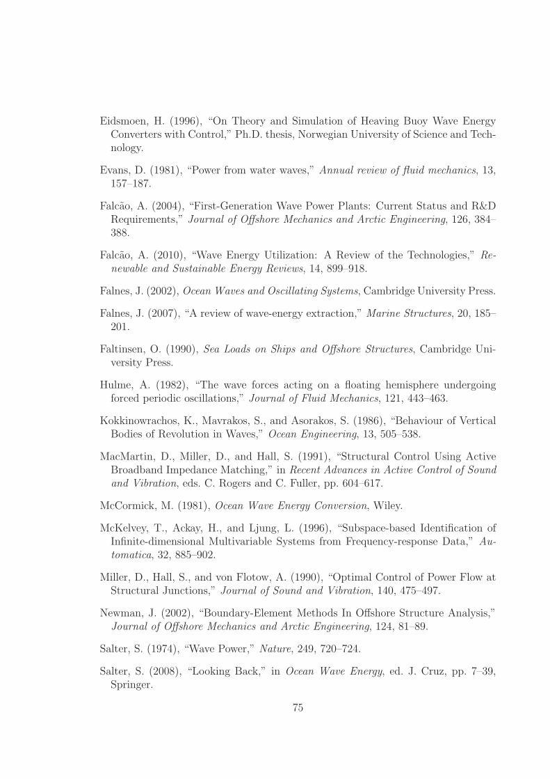
Eidsmoen, H. (1996), “On Theory and Simulation of Heaving Buoy Wave EnergyConverters with Control,” Ph.D. thesis, Norwegian University of Science and Tech-nology.
Evans, D. (1981), “Power from water waves,” Annual review of fluid mechanics, 13,157–187.
Falcao, A. (2004), “First-Generation Wave Power Plants: Current Status and R&DRequirements,” Journal of Offshore Mechanics and Arctic Engineering, 126, 384–388.
Falcao, A. (2010), “Wave Energy Utilization: A Review of the Technologies,” Re-
newable and Sustainable Energy Reviews, 14, 899–918.
Falnes, J. (2002), Ocean Waves and Oscillating Systems, Cambridge University Press.
Falnes, J. (2007), “A review of wave-energy extraction,” Marine Structures, 20, 185–201.
Faltinsen, O. (1990), Sea Loads on Ships and Offshore Structures, Cambridge Uni-versity Press.
Hulme, A. (1982), “The wave forces acting on a floating hemisphere undergoingforced periodic oscillations,” Journal of Fluid Mechanics, 121, 443–463.
Kokkinowrachos, K., Mavrakos, S., and Asorakos, S. (1986), “Behaviour of VerticalBodies of Revolution in Waves,” Ocean Engineering, 13, 505–538.
MacMartin, D., Miller, D., and Hall, S. (1991), “Structural Control Using ActiveBroadband Impedance Matching,” in Recent Advances in Active Control of Sound
and Vibration, eds. C. Rogers and C. Fuller, pp. 604–617.
McCormick, M. (1981), Ocean Wave Energy Conversion, Wiley.
McKelvey, T., Ackay, H., and Ljung, L. (1996), “Subspace-based Identification ofInfinite-dimensional Multivariable Systems from Frequency-response Data,” Au-
tomatica, 32, 885–902.
Miller, D., Hall, S., and von Flotow, A. (1990), “Optimal Control of Power Flow atStructural Junctions,” Journal of Sound and Vibration, 140, 475–497.
Newman, J. (2002), “Boundary-Element Methods In Offshore Structure Analysis,”Journal of Offshore Mechanics and Arctic Engineering, 124, 81–89.
Salter, S. (1974), “Wave Power,” Nature, 249, 720–724.
Salter, S. (2008), “Looking Back,” in Ocean Wave Energy, ed. J. Cruz, pp. 7–39,Springer.
75
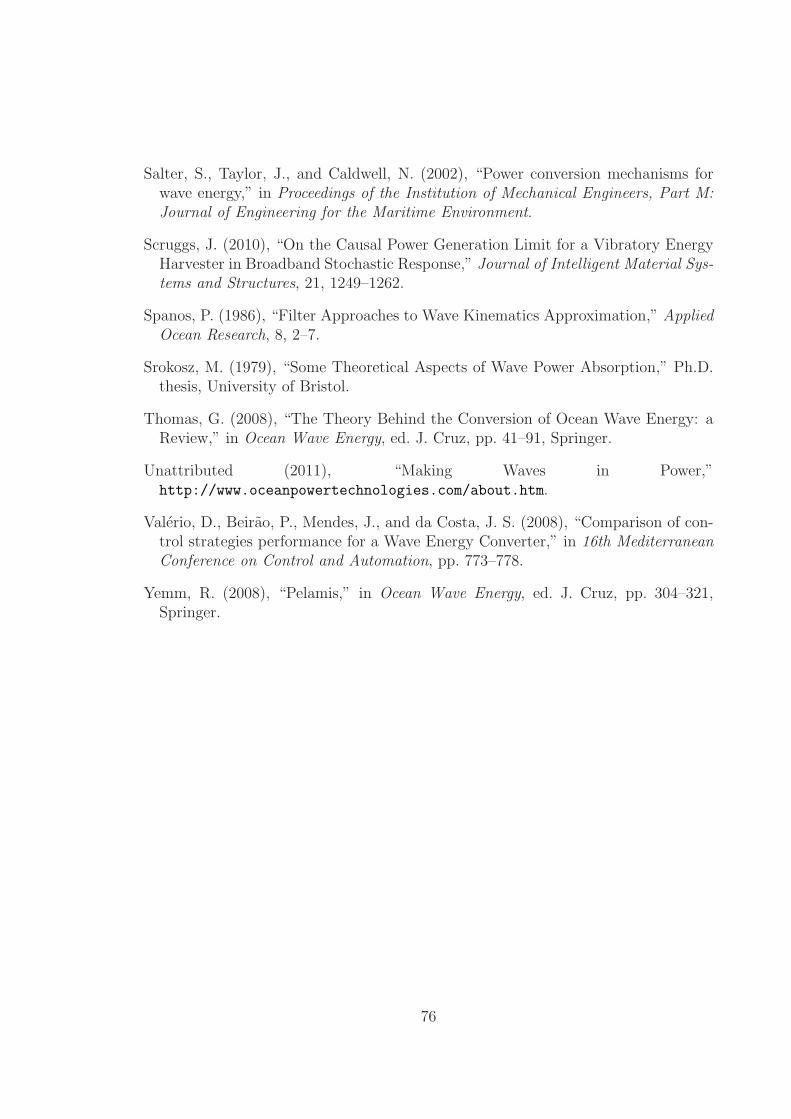
Salter, S., Taylor, J., and Caldwell, N. (2002), “Power conversion mechanisms forwave energy,” in Proceedings of the Institution of Mechanical Engineers, Part M:
Journal of Engineering for the Maritime Environment.
Scruggs, J. (2010), “On the Causal Power Generation Limit for a Vibratory EnergyHarvester in Broadband Stochastic Response,” Journal of Intelligent Material Sys-
tems and Structures, 21, 1249–1262.
Spanos, P. (1986), “Filter Approaches to Wave Kinematics Approximation,” Applied
Ocean Research, 8, 2–7.
Srokosz, M. (1979), “Some Theoretical Aspects of Wave Power Absorption,” Ph.D.thesis, University of Bristol.
Thomas, G. (2008), “The Theory Behind the Conversion of Ocean Wave Energy: aReview,” in Ocean Wave Energy, ed. J. Cruz, pp. 41–91, Springer.
Unattributed (2011), “Making Waves in Power,”http://www.oceanpowertechnologies.com/about.htm.
Valerio, D., Beirao, P., Mendes, J., and da Costa, J. S. (2008), “Comparison of con-trol strategies performance for a Wave Energy Converter,” in 16th Mediterranean
Conference on Control and Automation, pp. 773–778.
Yemm, R. (2008), “Pelamis,” in Ocean Wave Energy, ed. J. Cruz, pp. 304–321,Springer.
76