OPTIMAL PRICE DECREMENTAL STRATEGY FOR DUTCH …

COMMUNICATIONS IN INFORMATION AND SYSTEMS c© 2002 International PressVol. 2, No. 4, pp. 411-434, December 2002 006

OPTIMAL PRICE DECREMENTAL STRATEGY FOR DUTCH

AUCTIONS∗

WING HO YUEN† , CHI WAN SUNG‡ , AND WING SHING WONG§

Abstract. In a Dutch auction, the price of an item decreases incrementally from the starting

price at regular intervals. A bidder may buy the item at any time and stop the auction at the current

price. This paper presents an optimal price decrement strategy in a Dutch auction, such that the

expected revenue of the auction host is maximized. Properties of the optimal solution and a simple

iterative solution methodology are discussed. Numerical studies show that significant gain could be

obtained compared with a simple reference strategy.

Subject terms. Dutch auction; optimal auction; bidding; 3G; wireless application protocol;

optimization; time discounting; online auction;

Technical Subject Area. Mobile Internet: Applications and Technology, Personal Communi-

cations

1. Introduction. With recent advances in wireless standards, such as theIMT2000 for cellular networks as well as the HIPERLAN and the IEEE802.11 stan-dards for wireless local area networks, there has been great expectation that wirelessdata applications will soon become popular just like wireless telephony. In anticipa-tion of this development, there have been many attempts in testing pilot applicationson various wireless platforms. The Information Engineering Department at the Chi-nese University of Hong Kong has established a site, jawap.net, based on the WirelessApplication Protocol(WAP) to provide a host of wireless applications, including animplementation of a Dutch Auction System.

The Dutch auction is said to originate in the Netherlands and uses a descending-price format unlike the so-called “English Auction”. In the Dutch scheme, when anobject is presented to interested buyers for bidding the price will start at a high valueand progressively decreases downward until a buyer bids for the object by making adeclaration. If multiple declarations are made, any common resolution scheme canbe invoked to break the tie. It is possible to extend this scheme for the auctioningof multiple units of an object. Successful bidders bidding at the same price will eachreceive their unit at the bid price. If the number of units is not sufficient to cover

∗Received on May 22, 2002; accepted for publication on October 21, 2002. This work was partially

supported by a grant from the Area of Excellence in Information Technology in the Hong Kong Special

Administrative Region.†WINLAB, Rutgers University, Piscataway, NJ 08854-8060, USA. E-mail:

[email protected]‡Department of Computer Engineering and Information Technology, City University of Hong

Kong, Tat Chee Avenue, Hong Kong. E-mail: [email protected]§Department of Information Engineering, Chinese University of Hong Kong, Shatin, N.T., Hong

Kong. E-mail: [email protected]

411

412 WING HO YUEN, CHI WAN SUNG, AND WING SHING WONG

all the bids, a tie-breaking rule is invoked. If sufficient units of the object are stillavailable, the auction will continue until all the units are sold or a reserved price levelis reached.

The Dutch auction is one of the four major auctioning schemes ([1] or the surveyarticle [2],) that also include the English auction1, first price sealed bid auction2, andsecond price sealed bid auction (also known as the Vickrey auction)3. The seminalwork of Vickrey [3] analyzed and compared these four common kinds of auction rules.Since the process of an auction is very complicated involving the auctioneer, the seller,and multiple bidders, it is common to make certain simplifying assumptions aboutthese players in order to make the analytical model tractable. A key concept concernsthe idea of the value of the object under auction. The value can be private, that is, aperson buys an item for his/her own consumption without an objective to resell, orcommon, in which case the buyer bids with the intention of resell and has to estimatethe valuation offered by prospective buyers. In the latter case, the competitors areclearly a helpful source to obtain such a valuation estimate. A bidder is said to berisk neutral if he/she bids exactly accordingly to his/her evaluation of the object. Abidder who is likely to bid above his/her evaluation to increase the chance of winningis called a risk averse bidder.

Vickrey’s paper [3] assumes that each bidder is risk-neutral and knows the valueof the object to himself/herself but not the value to other bidders. Moreover, themodel is assumed to consist of symmetric bidders, that is, individual valuation ofthe object is i.i.d. Since then, there has been a steady output of follow-up work onoptimal auction design. One important piece of work was due to Myerson [4]. Heextended the work of Vickrey in two directions. Firstly, the case of asymmetric bid-ders is considered, in which individual valuations are independent but not necessarilyidentically distributed. Secondly, different viable ways of selling the object was con-sidered rather than just a prespecified set of auction rules. Under this framework,the optimal auction design problem to maximize the expected revenue of the auctionhost is solved. There have been many more additional works on the design of optimalauction rules. The well known auction rules are compared under various relaxationsof the stated assumptions [5], [6], [7].

With the advent of the World Wide Web, online auctions have become increas-ingly popular. Moreover, the arrival of 3G and high speed wireless local area networkshave made the idea of hosting auctions to serve mobile users via wireless communica-

1In the English auction, bidders compete with each other by offering progressively higher bids

until one bidder remains, who is committed to buy at last price of the last bid.2In a sealed bid auction, all the buyers submit a bid at the same time. The buyer offering the

highest bid is committed to buy the object the bid price.3In such an auction, the buyer making the highest bid is committed to buy the object, but at a

price equal to the second highest bid.

OPTIMAL PRICE DECREMENTAL STRATEGY FOR DUTCH AUCTIONS 413

tion devices, such as enhanced cellular phones or personal digital assistants, practicalin the near future. Coupled with the concept of micropayment, one can envision thepossibility of auctioning all sorts of items which may have only small monetary valueor are time-critical, such as tickets for an upcoming concert or seats on air flights.

For these applications, the expected time for completing an auction and theamount of signaling messages needed to conduct an auction are important consid-eration factors. These two elements are not considered in classical auctioning models.For Internet based auctions, in particular those available on wireless accesses, theissue of communication cost cannot be ignored. From this perspective, the Dutchauctioning scheme intuitively has an advantage over the English auctioning scheme.For the former scheme, no bidder is required to bid more than once, whereas for thelatter scheme bidders may have to bid several times whether they are successful atthe bidding or not. Moreover, although the possibility of multiple bids at the samevalue occurs in both cases, it can happen at most once in the auctioning process foran item in a Dutch scheme and multiple times for the English scheme.

Another motivation of our work comes from the observation that in the literature,a common assumption is that the bidding offers take values from a continuum. Thisis an idealization of an actual bidding process. In practice, bid increments in an En-glish auction or bid decrements in a Dutch auction is a discontinuous process. Whilea small discontinuous price decrement would minimize inaccuracies due to discreteoptimization, it would also prolong the auctioning process. For auctions conductedover the Internet, the value of a discontinuous decrement could have significant im-plications on the communication cost. In particular, for a Dutch auction, the optimalstrategy for price decrement is an interesting issue.

In this paper, we present an analysis of an Internet based Dutch auctioning sys-tem. In any auction, there are three player roles that one can consider, the buyer,the seller, and the auction host. Traditional analyses on auctioning tend to focus onthe roles played by the buyer or the seller. The role of the auction host is defined interms of the type of auctioning system used. For auctions conducted on Internet, theauction host is bestowed with a new set of controlling mechanisms and faces a newset of objectives. Assuming the revenue of the auction host comes from commissionbased on the realized bid revenue and the varying part of an auctioning cost is propor-tional to the duration of the bidding process, one can formulate an objective functionbased on these two factors. In a Dutch auction, an important controlling mechanismavailable to an auction host is through price decrement strategy. The structure ofthe optimal price decrement strategy in an Internet based Dutch auctioning system isanalyzed here via the Karush-Kuhn-Tucker condition. Moreover, we also establisheda numerically efficient algorithm to determine the optimal strategy. Numerical stud-ies were carried out and we showed that under certain conditions, the simple uniformdecrement strategy can be close to the optimal strategy. These results form a small,


first step to generalize the earlier works in the literature on auction in the new contextof the Internet based environment.

The rest of the paper is organized as follows. In section 2, we describe thesystem and optimization model. We maximize the expected revenue to the auctionhost by dynamically varying price decrement at each iteration. Knowledge on thenumber of bidders and the probability distributions of their valuations are exploited.In section 3, properties of the optimal solution are presented. We also show how theoriginal problem can be reduced to a one dimensional numerical search problem. Insection 4, we present numerical examples to illustrate the properties of the optimalsolution. Performance comparison between the optimal strategy and a simple uniformdecrement strategy is also given. Section 5 offers some concluding remarks.

2. System and Optimization Model.

2.1. System Model. In an auction, there are three distinct player roles, namelythe buyer, seller and auction host. In an Internet based auction, the auction host usu-ally acts as the application server and provides the necessary information to implementthe auction. It disseminates current price information to all bidders (logon users) reg-ularly, and ends the auction when it receives a buying request from the users or theauction timeout is reached.

We assume only one item is sold in the auction. Initially, the auction starts at agiven price c0. A price is kept constant for a fixed interval until the next iteration. Atiteration k, the price falls to ck, under the constraint cmin ≤ ck ≤ ck−1. The auctionwill last for M + 1 iterations, where M is predetermined.

Denote Xi as the valuation of bidder i. Let n be the number of bidders. Since theauction host is also the application server it knows the value of n. In this work, weassume n is constant for the duration of the auction. We also assume the valuationsof the ith bidder, Xi, for all i ∈ [1, n] are i.i.d. random variables drawn from a knowndistribution FX(.). In literature this is known as the case of symmetric bidders.However, our solution methodology also works for asymmetric bidders. This is thecase where bidder valuations are drawn from independent but not necessarily identicaldistributions.

Also denote Y = max(X1, ..., Xn) as the maximum valuations of the bidders. It isstraightforward to compute the cumulative distribution function cdf and probabilitydensity function pdf of Y for the cases of symmetric or asymmetric bidders. We denotethem by the notation F (Y ) and f(Y ) respectively. For simplicity, we assume thatf(Y ) is a continuous positive function in the range cmin, c0. Subsequently we willwork with Y directly since the sold price depends on the random variable Y . If thecurrent selling price ck is lower than Y , at least one user will immediately make a bidand end the auction. If cM > Y , the item will not be sold at the auction.


2.2. Optimization model. Suppose the item is sold at iteration k. ck is theselling price at iteration k, and T is a non-negative time discounting increment ateach iteration. Thus, the revenue is Rk = ck − kT if the item is sold at iterationk, k ∈ {0, ..., M}. If the item is not sold at the end of auction (i.e. cM > Y ), we definethe corresponding revenue as RM+1 = 0.

The expected revenue upon selling the item is

p(c) = Ek∈{0,...,M+1}[Rk](1)

= Ek∈{0,...,M}[ck − kT ](2)

= c0(1− F (c0)) +M∑

k=1

(ck − kT )(F (ck−1)− F (ck)).(3)

In our optimization model, we incorporated a time discounting factor T . Themeaning of T can be interpreted in two different scenarios. First of all, T can representthe cost of using server resources in a wireless Dutch auction. Typically, the auctionperiod spans only for minutes or hours. The auction server may update the price on aper minute or second basis. At each iteration, the application server has to broadcasta message to update the current price to all the clients (bidders). This generates a lotof data traffic and uses up bandwidth resources. Moreover, the amount of processingand bandwidth overhead can be regarded as being constant at each iteration. Thus,the resource usage is adequately modeled by a constant parameter T .

Alternatively, this model can also apply to online auction websites where auctionperiod spans over longer periods of time, such as days or weeks. It is common in thesecases that the price of an item is dropped gradually on a daily basis. In this scenario,the amount of network traffic generated is insignificant. Rather, there is a timediscounting factor on the value of the good to account for storage and maintenancecost incurred on the auction host.

The present problem belongs to a class of general nonlinear optimization problemswith inequality constraints. The problem is to

max(c1,c2,...,cM )

p(c) = max(c1,c2,...,cM )

c0(1− F (c0)) +M∑

k=1

(ck − kT )(F (ck−1)− F (ck)

)

subject to the constraints

(4)

g1(c) = c1 − c0 ≤ 0,

g2(c) = c2 − c1 ≤ 0,...gM (c) = cM − cM−1 ≤ 0,

gM+1(c) = cmin − cM ≤ 0.

We note that many alternative formulations such as dynamic programming [8]are possible. Our nonlinear programming formulation is desirable for practical imple-


mentation because, as we will show in the next section, the multivariable optimizationproblem of determining the selling price M -tuple ck, k = 1, 2, ..., M can be reducedto a one dimensional numerical search problem. Since an auction host typically hashundreds or thousands of items for sale, the reduction of computation complexity inprice setting is desirable for running a large auction hosting site.

3. Properties of the optimal solution. In the literature, optimization ofnonlinear functions subject to inequality constraints is well studied. The Karush-Kuhn-Tucker (KKT) Theorem is one of the powerful tools commonly employed.

Let c be any point in the feasible set. Denote J(c) = {j : gj(c) = 0}. If ∇gj(c)are mutually linearly independent for all j ∈ J(c), then c is a regular point. The wellknown theorem due to Karush,Kuhn and Tucker [9] provides a necessary conditionfor a point to be a local maximizer, commonly known as the Karush-Kuhn-Tucker(KKT) condition, presented as follows.

Let c∗ be a regular point and local maximizer for the problem of maximizing p subjectto g(c) ≤ 0. Then there exists a vector u∗ ∈ <M+1 such that

u∗ ≥ 0(5)

∇p(c∗) = ∇g(c∗)u∗(6)

u∗T g(c∗) = 0(7)

where

(8) u∗ =

u∗1u∗2...

u∗M+1

g(c∗) =

g1(c∗)g2(c∗)

...gM+1(c∗)

,

and ∇g(c∗) is the M ×M + 1 matrix whose i-th column is ∇gi(c∗).We refer to the vector u∗ as the Karush-Kuhn-Tucker (KKT) multiplier vector. In

the literature, a point satisfying the KKT condition (equation 5-7) is called a criticalpoint. It follows from the KKT Theorem that a local maximizer is a critical point butnot necessarily vice versa. We also define the global maximum in the feasible set asc∗∗. Thus, if c∗∗ is regular, it is also within the set of all critical points.

For the stated optimization problem, the constraint stated by equation 4 can berewritten as:

(9) g(c) =

c1 − c0

c2 − c1

...cmin − cM

.


Therefore,

(10) ∇g(c) =

1 −1 0 · · · 0 0 00 1 −1 · · · 0 0 00 0 1 · · · 0 0 0...

......

. . ....

......

0 0 0 · · · −1 0 00 0 0 · · · 1 −1 00 0 0 · · · 0 1 −1

.

It is obvious that any selection of M column vectors from∇g are mutually linearlyindependent. Hence any point, c, in the feasible set with the cardinality of J(c) lessthan M +1 is a regular point. The case where J(c) = {1, 2, ...,M +1} corresponds toc0 = c1 = ... = cM = cmin, does not belong to the feasible set since c0 6= cmin. Thus,every point in the feasible set is regular. It follows from KKT Theorem that all localmaxima are regular and should satisfy the KKT equations. As a result, c∗∗ can befound by searching over the set of all critical points. Hereafter, we denote a criticalpoint by c∗.

On substitution of g(c∗) and ∇g(c∗) into equation 6, one obtains

∇p(c∗) =(

∂p∂c1

(c∗), ∂p∂c2

(c∗), . . . , ∂p∂cM

(c∗))

=(

u∗1 − u∗2, u∗2 − u∗3, . . . , u∗M − u∗M+1

).(11)

The last KKT condition in equation 7 leads to the conclusion

u∗kgk(c∗) = u∗k(c∗k − c∗k−1) = 0, for k = 1, 2, ..., M + 1.(12)

since c∗k − c∗k−1’s are non-positive for all k.There are standard algorithmic approaches to solve the class of convex program-

ming problems in which the objective function is concave and the feasible set is convex.However, we show in the appendix that our objective function is not concave in gen-eral. As a result, local search technique is applied to identify local maxima. Thesearch procedure is repeated with different initial points to discover as many distinctlocal maxima as possible. The best of these local maxima is chosen as the solution.Numerical computations for this heuristic approach over the feasible set for local max-ima can be quite extensive. This is an important consideration when the number ofiterations is large. In this case an optimization problem in M variables needs to beconsidered. However, it turns out that by exploiting our knowledge of the structureof the critical points, we could determine the global optimum c∗∗ by reducing theproblem to a one dimensional search problem. This is the main result provided bytheorem 3. In the following, we present some basic properties of the optimal solutionand describe an iterative solution methodology for finding the global maximum c∗∗.


Suppose one implements an auction following the optimal price vector c∗∗. Atiteration j, the current price is c∗∗j . Define the subproblem starting at iteration j asone in which there are M − j remaining iterations, starting from the price c∗∗j . Theproblem of finding the optimal price vector for this problem is equivalent to solvingthe problem,

max(cj+1,...,cM )

Ek∈{j+1,...,M+1}[Rk|Y < c∗∗j ](13)

= max(cj+1,...,cM )

Ek∈{j+1,...,M}[ck − kT |Y < c∗∗j ].(14)

Proposition 1. For any j, j ∈ {1, ..., M−1}, (c∗∗j+1, c∗∗j+2, . . . , c

∗∗M ) is the optimal

price vector to subproblem starting at iteration j.

Proof.

max(cj+1,cj+2,...,cM )

Ek∈{j+1,...,M}[ck − kT |Y < c∗∗j ](15)

= max(cj+1,cj+2,...,cM )

M∑

k=j+1

(ck − kT )(F (ck−1)− F (ck))

F (c∗∗j )(16)

=1

F (c∗∗j )max

(cj+1,cj+2,...,cM )

M∑

k=j+1

(ck − kT )(F (ck−1)− F (ck)).(17)

It is obvious that the above expression is optimized when ck = c∗∗k for k =j + 1, ...,M .

The previous result states that if the number of bidders n is constant throughoutthe auction period, then we need to compute c∗∗ only once at the start of the auction.In practice, n may change from time to time as bidders may join or leave during anauction. In that case, one needs to get an update on the value of nj at iteration j

and computes the new optimal price vector.

When the number of iterations M is large, numerical optimization becomes morecomplicated due to the number of variables involved. In theorem 1 and 3, we showthat the multivariable optimization problem can be reduced to a one dimensionalsearch problem.

Theorem 1. Suppose c∗ is a critical point and there exists an integer i such thatc∗i = c∗i+1, where i = {0, 1, ..., M − 1}. Then for all j > i, j ∈ {i+1, ..., M}, c∗i = c∗j .

Proof. Any feasible point must satisfy the condition:

(18) c0 ≥ c∗1 ≥ ... ≥ c∗k ≥ c∗k+1 ≥ ... ≥ c∗M ≥ cmin.

We claim that there does not exist an integer i, 0 ≤ i ≤ M−2, and a j, i < j ≤ M−1,such that:

(19) c0 > c∗1 > ... > c∗i = c∗i+1 = ... = c∗j > c∗j+1 ≥ ... ≥ cM ≥ cmin.


We prove this statement by contradiction. By the Karush-Kuhn-Tucker Theoremwe have to find u∗ ≥ 0 so that equations 5-7 are satisfied. For convenience, we definethe functions h and hM as

h(ck−1, ck, ck+1) =∂p

∂ck(20)

= F (ck−1)− F (ck) + f(ck)(ck+1 − ck − T ) k ∈ {1, . . . , M − 1},(21)

hM (cM−1, cM ) =∂p

∂cM(22)

= F (cM−1)− F (cM ) + (cM −MT )(−f(cM )).(23)

Since gk(c∗) < 0 for k ∈ {1, ..., i}, by equation 12,

u∗k = 0, k ∈ {1, ..., i}.(24)

At the point c∗, by equation 11 the following equations hold:

(25)

∂p∂ck

(c∗) = h(c∗k−1, c∗k, c∗k+1) = u∗k − u∗k+1 = 0, k ∈ {1, ..., i− 1},

∂p∂ci

(c∗) = h(c∗i−1, c∗i , c

∗i+1) = −u∗i+1,

∂p∂ci+1

(c∗) = h(c∗i , c∗i+1, c

∗i+2) = u∗i+1 − u∗i+2,

...∂p

∂cj−1(c∗) = h(c∗j−2, c

∗j−1, c

∗j ) = u∗j−1 − u∗j ,

∂p∂cj

(c∗) = h(c∗j−1, c∗j , c

∗j+1) = u∗j − u∗j+1.

Since

gj+1(c∗) = c∗j+1 − c∗j < 0,(26)

equation 12 implies that u∗j+1 = 0.

∂p

∂cj(c∗) = u∗j − u∗j+1 = u∗j(27)

= h(c∗j−1, c∗j , c

∗j+1)(28)

= F (c∗j−1)− F (c∗j ) + f(c∗j )(c∗j+1 − c∗j − T )(29)

= f(c∗j )(c∗j+1 − c∗j − T )(30)

< 0.(31)

That is u∗j < 0, hence the non-negativity condition on u∗ is not satisfied. By contra-diction we show that the scenario stated in equation 19 cannot hold.

Corollary 1. Suppose c∗ is a critical point and

(32) c0 > c∗1 > ... > c∗i = c∗i+1 = ... = c∗M ≥ cmin.


for some 0 ≤ i < M . Then

(33)∂p∂cj

(c∗) = 0 j ∈ {1, ..., i− 1},∂p∂cj

(c∗) ≤ 0 j ∈ {i, ..., M − 1}.

Proof. The proof of theorem 1 shows that

(34)∂p

∂ci(c∗) = −u∗i+1 ≤ 0.

Since c∗i = c∗i+1 = ... = c∗M , we observe that

∂p

∂ci+1(c∗) =

∂p

∂ci+2(c∗) = ... =

∂p

∂cM−1(c∗)(35)

= h(c∗i , c∗i+1, c

∗i+2)(36)

= F (c∗i )− F (c∗i+1) + f(c∗i+1)(c∗i+2 − c∗i+1 − T )(37)

= −Tf(c∗i+1)(38)

≤ 0.(39)

We now introduce the notation of a sequence-valued function

(40) c(s) = (c0, c1, c2, ..., cM ) = (c0, s, c2, ..., cM ).

The domain for s is defined in the range cmin ≤ s ≤ c0. The elements of c are definedrecursively in the following way:

Assume that elements up to ck have been defined. Let t be the solution to:

(41) h(ck−1, ck, t) = 0.

(Note that by our assumption on the pdf and the definition of h, t always exists andis unique.) If cmin ≤ t ≤ ck and t − (k + 1)T > 0, then ck+1 = t. Otherwise, defineck+1 = ck.

Note that c(s) defines a 1-parameter family of critical points satisfying the KKTconditions. However, not all critical points can be represented by c(s) for some s.Suppose c∗ is a critical point and

(42) c0 > c∗1 > ... > c∗i = c∗i+1 = ... = c∗M ≥ cmin

for some 0 ≤ i < M . If c∗1 = c1, then it follows directly from equation 25 and thedefinition of c that

c∗k = ck k ∈ {1, ..., i− 1}.(43)

However, c∗k and ck, for k ≥ i, may not be equal. In general,

c∗k ≥ ck k ∈ {i, ..., M − 1}.(44)


To show that an optimal solution can be obtained by searching the family ofcritical points defined by c(s), we need the following observation:

Theorem 2. Define Rj = c∗∗j − jT , for j ∈ {1, . . . , M}. If Rj ≤ 0, thenc∗∗k = c∗∗k−1 for k ∈ [j,M ]. If Rj > 0, then c∗∗j < c∗∗j−1 if c∗∗j−1 > cmin.

Proof. Suppose Rj < 0. We have RM ≤ RM−1 ≤ ... ≤ Rj+1 ≤ Rj < 0.

p(c) =M∑

k=1

Rk(F (ck−1)− F (ck))(45)

=j−1∑

k=1

Rk(F (ck−1)− F (ck)) +M∑

k=j

Rk(F (ck−1)− F (ck)).(46)

If c∗∗k < c∗∗k−1 for any k ∈ [j, M ], p can be increased by setting c∗∗k = c∗∗k−1 for k ∈ [j, M ].A contradiction.

Suppose Rj = 0 and c∗∗j < c∗∗j−1. p can be increased by changing c∗∗j to anyvalue in the interval (c∗∗j , c∗∗j−1), and setting c∗∗k = c∗∗k−1 for k ∈ [j + 1,M ]. Again acontradiction.

On the other hand, suppose Rj > 0. If c∗∗j = c∗∗j−1 then all c∗∗k ’s must be equalfor k ≥ j according to theorem 1. Therefore, p(c) can be increased by setting c∗∗j toa value in the interval (cmin, c∗∗j−1) while keeping Rj > 0. A contradiction. Hence,c∗∗j < c∗∗j−1.

Now we are ready to prove our main result:Theorem 3. If c∗∗ is an optimal solution, then c(s) = c∗∗ when s = c∗∗1 .Proof. Suppose c∗∗ = (c∗∗0 , c∗∗1 , . . . , c∗∗M ) is an optimal solution. Set s = c∗∗1 .Define Rj = c∗∗j − jT . Suppose Rj > 0 for all j ∈ {2, . . . , M}, then it follows

from corollary 1 and theorem 2 that c∗∗j−1 > c∗∗j and h(cj−2, cj−1, cj) = 0 unlessc∗∗j−1 = cmin. It follows from the definition of c(s) that

(47) ck = c∗∗k

for all k.Suppose Rj ≤ 0 for some j ∈ {2, . . . , M}. If j < M , notice that c∗∗M = c∗∗M−1 =

. . . = c∗∗j since Rk < 0 for k > j. Hence, it follows from the definition of c(s) that

(48) ck = c∗∗k

for all k.According to this theorem, by doing a one-dimensional numerical search for c(s)

within the feasible set, one can obtain an optimal solution to the problem. We nowdescribe two more observations on the structure of the optimal solution. First of all,the following theorem shows that depending on whether F (.) is convex or concave, thesequence of price difference of the optimal strategy, c∗∗k − c∗∗k+1, satisfies the followinginequalities.


Theorem 4. Given c∗∗ with the form c0 > c∗∗1 > ... > c∗∗i = c∗∗i+1 = ... = c∗∗M ≥cmin. If F (.) is convex in [cmin, c0], then

c∗∗k−1 − c∗∗k ≤ c∗∗k − c∗∗k+1 + T k ∈ {1, ..., i− 1}.(49)

If F (.) is concave in [cmin, c0], then

c∗∗k−1 − c∗∗k ≥ c∗∗k − c∗∗k+1 + T k ∈ {1, ..., i− 1}.(50)

Proof. By Corollary 1,

∂p

∂ck(c∗∗) = 0 k ∈ {1, ..., i− 1}.

That is,

F (c∗∗k−1)− F (c∗∗k ) + f(c∗∗k )(c∗∗k+1 − c∗∗k − T ) = 0.(51)

Consider the case when F (.) is convex.

F (c∗∗k−1)− F (c∗∗k )c∗∗k−1 − c∗∗k

≥ f(c∗∗k )(52)

or

F (c∗∗k−1)− F (c∗∗k ) + f(c∗∗k )(c∗∗k − c∗∗k−1) ≥ 0.(53)

Subtracting equation 51 from equation 53, we have

f(c∗∗k )[(c∗∗k − c∗∗k−1)− (c∗∗k+1 − c∗∗k − T )

] ≥ 0(54)

or

c∗∗k−1 − c∗∗k ≤ c∗∗k − c∗∗k+1 + T.(55)

The case when F (.) is concave can be proven in the same way.

When X is uniformly distributed as U(a, b), the pdf of Y is convex. In the specialcase T = 0, we note that the price difference c∗∗k −c∗∗k+1 is increasing with time, whereasthe probability F (c∗∗k ) − F (c∗∗k+1) is decreasing. This conforms to our intuition thatprice levels should be closely packed at intervals where pdf of Y is large, such thatthe item could be sold at a price ck close to Y .

When X is normal distributed as N(µ, σ2),

F (y) = Q

(µ− y

σ

)n

,(56)

f(y) = nQ

(µ− y

σ

)n−1 1√2πσ

exp(−(µ− y)2

2σ2).(57)


It could be shown that F (y) is convex when y ≤ ψ and concave otherwise, where ψ

is solution to the equation

(n− 1) exp(−x2

2) +

√2πxQ(x) = 0, x =

(µ− ψ)σ

.(58)

Since the pdf of Y is largest at ψ, the price difference is decreasing at first and startsincreasing again as c∗∗k passes through ψ. That is, price levels are more closely packedaround Y = ψ.

A uniform price decrement strategy is used as a reference in the numerical studies.The price vector starts at c0 and falls to cmin in M equally spaced steps. We hereafterrefer this strategy as the uniform price decrement strategy. It turns out that thisstrategy is optimal in the trivial case as shown in the following theorem.

Theorem 5. Uniform decrement strategy is optimal when(1)X ∼ U(a, b), c0 ≤ b and a ≤ cmin

(2) n = 1,(3) T = 0.

The optimal price levels are given by

c∗∗k =(

M − k

M

)c0 −

(k

M

)cmin, cmin ≥ c0

M + 1,(59)

c∗∗k =(

M + 1− k

M + 1

)c0, cmin ≤ c0

M + 1.(60)

Proof. We will show that c∗∗ defined in equation 59 and equation 60 satisfiesthe KKT conditions. Then we prove that p is concave in the feasible set. Since p isconcave, the optimality of c∗∗ is proved.

F (y) =

{y−ab−a a ≤ y ≤ b

0 otherwisef(y) =

1b− a

a ≤ y ≤ b.

Substitute to equation 3 we have

p =1

b− a

M∑

k=1

ck(ck−1 − ck).(61)

Taking partial derivatives w.r.t. ck

∂p

∂ck=

1b− a

[(ck−1 − ck)− (ck − ck+1)] k ∈ {1, ..., M − 1},(62)

∂p

∂cM=

1b− a

(cM−1 − 2cM ).(63)

Consider the case cmin ≥ c0M+1 . Substitute the price vector c∗∗ (equation 59) to


equation 62, we have

∂p

∂ck(c∗∗) = 0 k ∈ {1, ..., M − 1},(64)

∂p

∂cM(c∗∗) =

1b− a

[−cmin +

(c0 − cmin

M

)](65)

=1

b− a

[M − 1

M(

c0

M + 1− cmin)

](66)

≤ 0.(67)

gk(c∗∗) < 0 ∀k ∈ {1, ...,M}. By construction u∗k = 0, k ∈ {1, ..., M}, so thatequation 12 is satisfied. Moreover, u∗∗M+1 ≥ 0. Thus we have

∂p

∂ck(c∗∗) = u∗∗k − u∗∗k+1 = 0 k ∈ {1,M − 1},(68)

∂p

∂cM(c∗∗) = u∗∗M − u∗∗M+1(69)

= −u∗∗M+1 ≤ 0.(70)

Thus the KKT condition 2 is also satisfied. Therefore there exists a non-negative u∗

that satisfies all the KKT conditions.Consider the case cmin ≤ c0

M+1 . We substitute the price vector c∗∗ (equation 60)to equation 62, yielding

∂p

∂ck(c∗∗) = 0 k ∈ {1, ..., M − 1},(71)

∂p

∂cM(c∗∗) =

1b− a

(c∗∗M−1 − 2c∗∗M )(72)

= 0(73)

on simplification. Since gk(c∗∗) < 0 for k ∈ {1, ..., M +1}, by equation 12 u∗∗k = 0, k ∈{1, ..., M + 1} . Thus we have u∗∗k − u∗∗k+1 = 0. All the KKT conditions are satisfiedagain for this c∗∗.

To show that c∗∗ is a global maximizer, we proceed to prove the Hessian matrixH for the objective function p is negative semi-definite. It is trivial to show that

H =1

b− a

−2 1 0 · · · · · · 01 −2 1 0 · · · 00 1 −2 1 · · · 0

. . . . . . . . . 00 · · · 1 −2 1 00 · · · 0 1 −2 10 · · · · · · 0 1 −2

.

Apply the Gerschgorin’s theorem on each row of H, we show that max(λ) ≤ 0. Thus,H is negative semi-definite and p is concave.


So far Theorem 3 is the most important observation. Suppose an auction hostknows the statistics of the individual valuation F . The auction host only needs tosearch for different values of s for the optimal value c∗∗1 . The nature of the optimizationproblem stipulates that if s = c∗∗1 , then c∗∗ = c(s) is the optimum solution to theoptimization problem. Given s, c(s) can be determined easily by recursively solvingsimple algebraic equations (41) M − 1 times. Thus, an exhaustive search of s leadsto the solution for the optimal price settings.

4. Numerical Studies. In this section, we firstly present several numerical ex-amples to illustrate the properties of c∗∗. Then, the optimal strategy is compared tothe uniform price decrement strategy in the following subsection.

4.1. Illustration of properties of optimal solution. In figure 1, X is uni-formly distributed as U(700, 1000). There is no discounting factor, i.e. T = 0. Theoptimal price c∗∗k at iteration k is plotted for n = 1, 5, 10, 20, 50 respectively. Whenn = 1, we observe that the uniform decrement strategy is optimal. Since cmin ≥ c0

M+1 ,c∗∗ is given by equation 59. As n increases, the pdf of Y shifts to the right. Thusthe price decrement rate is more gradual. When n = 20, cM is approximately equalto 870. When n = 50, cM is approximately equal to 930. In both cases, we note thatthe probability Pr[Y ≤ cM ] is very small. We also observe that the cost differencec∗∗k − c∗∗k−1 is increasing with k. The observation is in agreement to equation 49 sinceFY (y) is convex.

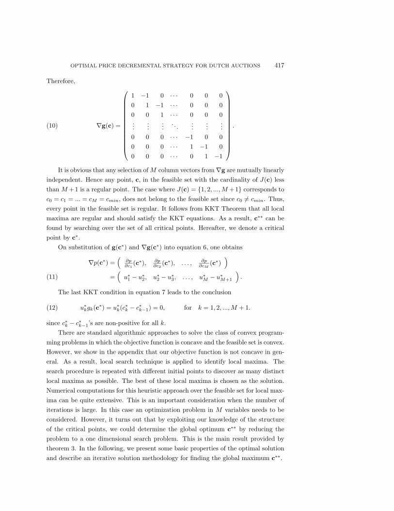
In the following examples, we assume the valuation of a bidder X is normaldistributed with mean 850 and variance 502. The pdf of maximum valuation Y fordifferent n is shown on figure 2. Note that the pdf becomes more peaked and shiftsto the right as n increases. Figure 3 shows the case when T = 0 and X is normaldistributed as N(850, 502). For all values of n, the price difference is decreasing at firstand increasing towards the end. This agrees with our results for normal distributedX’s, since F (Y ) changes from convex to concave as Y increases. When n = 1, the pdfis maximum around µ = 850. Thus, the initial drop in price is fast. After that, thedrop in price is about the same in each iteration. On the other hand, when n = 50,the pdf is maximum around 960 and tends to zero around 900. Thus, the drop inprice is slowest around 960 and becomes faster after it passes through the pdf maxima.Note that for n = 10, 20, 50, the iterations end essentially at the point when the pdfis essentially zero.

In figure 4, a discounting factor of T = 20 is introduced in each iteration. Theprice c∗∗k at iteration k is plotted for the cases n = 1, 5, 10, 20, 50. We observe theinclusion of a non-zero discounting factor T leads to faster price decrements. Asone can read from figure 2, the maxima of f(Y ) occur around 850, 900, 920, 940, 960respectively when n = 1, 5, 10, 20, 50. The optimal price decrement c∗∗1 lies in thevicinity of these pdf maxima. We note that when n = 50, the simulation result is


0 2 4 6 8 10 12 14 16 18 20

800

820

840

860

880

900

920

940

960

980

1000

Number of iterations i

Pric

e C

(i)

X~U(700,1000), (Cmin,C0)=(800,1000), n=1,5,10,20,50, T=0, M=20

n=50

n=20

n=10

n=5

n=1

Fig. 1. Example 1: X uniformly distributed, T = 0

suboptimal. The auction ends at iteration 15 at a price higher than cmin. Thus,the expected revenue can be further increased by additional price decrements. Thediscrepancy is due to numerical inaccuracies that occur at iterations when the pdf ofY at the selling price is extremely small. In this case, the pdf of Y around c15 is lessthan 10−9. Despite the numerical inaccuracies, the proposed method tends to yieldsolutions that are nearly optimal since the difference in the expected revenue is small.

In figure 5, we change the discount factor to T = 50. The optimal price decrementsfor different n are shown. As predicted, the price decrement is even steeper comparedto the cases where T = 20 and T = 0. In the case n = 20 and n = 50, the iterativesolution fails to touch cmin when the auction ends due to the resolution inaccuracyin the search. Again, a nearly optimal solution is obtained since the pdf when theauction ends is very small (less than 10−10).

In figure 6, the price decrements are compared for different discounting factorT = 0, 5, 10, 20, 50. The number of bidders is n = 10. As T increases, the pricedecrement is steeper. Thus, if the resource usage is expensive, the auction host wouldprefer a strategy with faster price decrements.


800 820 840 860 880 900 920 940 960 980 10000

0.002

0.004

0.006

0.008

0.01

0.012

0.014

0.016

0.018

0.02

X~N(850,502), pdf of Y=max(X1,...,X

n)

n=50

n=20

n=10

n=5

n=1

Fig. 2. pdf of Y for n = 1, 5, 10, 20, 50

Table 1

Revenue ratio of the optimal and the reference strategy when T and n are varied.

n 1 5 10 20 50

T = 0, X ∼ U(700, 1000) 1.0000 1.0012 1.0027 1.0042 1.0058

T = 0, X ∼ N(850, 502) 1.0009 1.0012 1.0018 1.0023 1.0028

T = 20, X ∼ N(850, 502) 1.3920 1.2033 1.1444 1.1000 1.0566

T = 50, X ∼ N(850, 502) 4.8749 1.9413 1.5764 1.3655 1.1948

4.2. Comparison with the uniform decrement strategy. Comparison isdone in terms of the expected revenue p. The ratio p(c∗∗)/p(cref ) is shown in Table1. We also compare the expected time to sell an item, as shown in Table 2. Supposea strategy c is used. Define the expected time to sell an item Ts, given that it isactually sold when the auction ends as E[Ts|Y ≥ cM ]. It is straightforward to showthat

E[Ts|Y ≥ cM ] =∑M

k=1 k(F (ck−1)− F (ck))1− F (cM )

(74)

=∑M−1

k=0 F (ck)−MF (cM )1− F (cM )

.(75)


0 2 4 6 8 10 12 14 16 18 20

800

820

840

860

880

900

920

940

960

980

1000


Pric

e C

(i)

X~N(850,502), (Cmin,C0)=(800,1000), n=1,5,10,20,50, T=0, M=20

n=50

n=20

n=10

n=5

n=1

Fig. 3. Example 2: X normal distributed, T = 0

Table 2

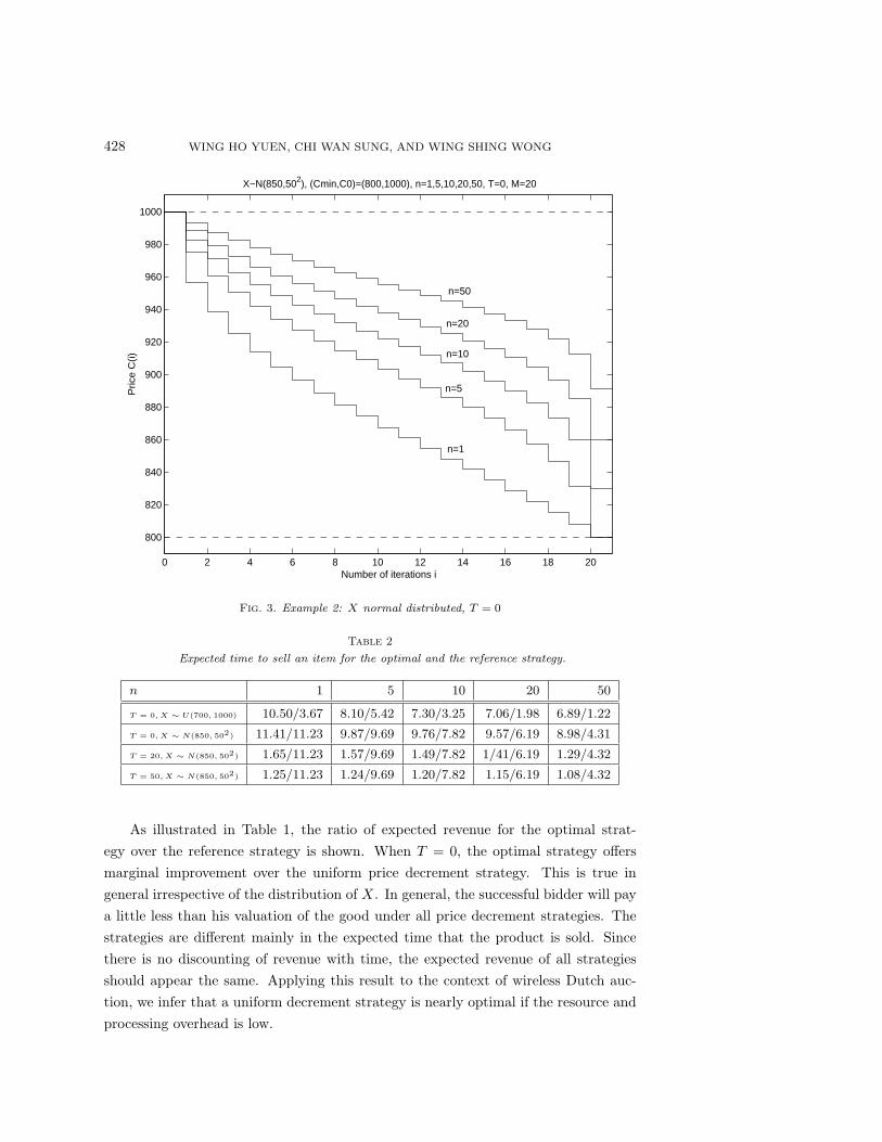
Expected time to sell an item for the optimal and the reference strategy.

n 1 5 10 20 50

T = 0, X ∼ U(700, 1000) 10.50/3.67 8.10/5.42 7.30/3.25 7.06/1.98 6.89/1.22

T = 0, X ∼ N(850, 502) 11.41/11.23 9.87/9.69 9.76/7.82 9.57/6.19 8.98/4.31

T = 20, X ∼ N(850, 502) 1.65/11.23 1.57/9.69 1.49/7.82 1/41/6.19 1.29/4.32

T = 50, X ∼ N(850, 502) 1.25/11.23 1.24/9.69 1.20/7.82 1.15/6.19 1.08/4.32

As illustrated in Table 1, the ratio of expected revenue for the optimal strat-egy over the reference strategy is shown. When T = 0, the optimal strategy offersmarginal improvement over the uniform price decrement strategy. This is true ingeneral irrespective of the distribution of X. In general, the successful bidder will paya little less than his valuation of the good under all price decrement strategies. Thestrategies are different mainly in the expected time that the product is sold. Sincethere is no discounting of revenue with time, the expected revenue of all strategiesshould appear the same. Applying this result to the context of wireless Dutch auc-tion, we infer that a uniform decrement strategy is nearly optimal if the resource andprocessing overhead is low.


0 2 4 6 8 10 12 14 16 18 20

800

820

840

860

880

900

920

940

960

980

1000

X~N(850,502), (Cmin,C0)=(800,1000), n=1,5,10,20,50, T=20, M=20


Pric

e C

(i)

n=50

n=20

n=10 n=5

n=1


When the discounting factor is non-zero, the optimal strategy outperforms thealternate strategy by a large margin. In our studies, the difference is more remarkablewhen n is small or T is large. When T is large, it is desirable to sell an item soonerto reap more profits. Reading from Table 2, the expected time to sell the good ismuch shorter for the optimal strategy. Thus, the optimal strategy is significantlybetter when T is large. In a wireless Dutch auction, it is reasonable to assume thenumber of bidders n = 5 or n = 10. For the case T = 50, the optimal strategy issuperior to the uniform strategy by 94% and 57% respectively as read from Table 1.Thus, in a wireless Dutch auction, we should refrain from using the uniform strategyif communication resources are expensive. Similarly, when the value of a good suffersfrom fast time discounting, as in perishable goods such as Dutch tulips, the uniformstrategy should not be used.

From figure 2 we observe that the pdf shifts to the low price region when n issmall. For the uniform decrement strategy, it takes many iterations until the item issold. Thus the revenue suffers from large time discounting. In the optimal strategy,the initial price decrements are steep so that the maximum valuation is reached uponseveral iterations. In practice, a Dutch auction is usually started at a very high initialprice c0 À Y > cmin. The maximum valuation Y is substantially below c0. The use


0 2 4 6 8 10 12 14 16 18 20

800

820

840

860

880

900

920

940

960

980

1000


Pric

e C

(i)

X~N(850,502), (Cmin,C0)=(800,1000), n=1,5,10,20,50, T=50, M=20

n=50

n=20

n=10 n=5 n=1


of the optimal strategy leads to significant gain over the uniform decrement strategyby significantly shortening the auction time and the corresponding amount of timediscounting.

We have demonstrated that when the time discounting factor T is large andwhen the number of bidders n is small, the optimal strategy have the potential tooutperform the uniform decrement strategy by a large margin. The underlying reasonfor the performance difference is that the auction time is significantly shortened forthe optimal strategy as illustrated in Table 2. More generally, when parameters suchas cmin, σ and M are varied, the auction time may be adversely prolonged by usingthe uniform decrement strategy. Thus under certain parameter settings, we alsoobserve a large performance margin between the optimal and the uniform decrementstrategy. Specifically, when the lower price limit cmin and individual valuations Xi aresmall compared with the initial price c0, the auction time for the reference strategyis considerably longer. Similarly, when the variance of the individual valuations σ issmall, the maximum valuation over all bidders Y is also smaller, thus prolonging theauction time of the uniform decrement strategy. Finally, when the number of allowediterations M in an auction increases, the resultant price decrement interval of theuniform strategy is finer. This also adversely affect the performance of the reference


0 2 4 6 8 10 12 14 16 18 20

800

820

840

860

880

900

920

940

960

980

1000


Pric

e C

(i)

X~N(850,502), (Cmin,C0)=(800,1000), T=0,5,10,20,50, n=10, M=20

T=50

T=20

T=10

T=5

T=0

Fig. 6. Example 5: X normal distributed, n = 10

strategy relative to the optimal strategy.

Table 3

Revenue ratio of the optimal and the reference strategy when cmin, σ and M are varied.

Parameters revenue ratio

T = 10, n = 10, cmin = 100, M = 20, σ = 50, X ∼ N(300, 502) 1.6168

T = 10, n = 10, cmin = 100, M = 20, σ = 100, X ∼ N(300, 502) 1.3256

T = 10, n = 10, cmin = 100, M = 20, σ = 25, X ∼ N(300, 502) 1.8736

T = 10, n = 10, cmin = 100, M = 10, σ = 25, X ∼ N(300, 502) 1.5414

T = 10, n = 10, cmin = 100, M = 30, σ = 25, X ∼ N(300, 502) 2.3685

As a simple illustration we consider 5 more numerical examples with results shownin Table 3. In all the five examples, the lower price limit is cmin = 100. Individualvaluations are modeled as i.i.d. Gaussian random variables with mean µ = 300 andvariance σ2 = 502. The revenue ratio of the optimal strategy relative to the uni-form decrement strategy is found to be more than 60%. This confirms our intuitionthat when c0 À Y > cmin, the optimal strategy outperforms the reference strategyby a large margin. In the second and third examples, the variance of the individ-


ual valuations is varied as σ2 = 1002 and σ2 = 252 respectively. The correspondingrevenue ratios are 1.3256 and 1.8736. Our results show that as the variance σ2 in-creases, the revenue ratio also increases. When the valuations of the bidders showsmaller randomness, it is unlikely that the maximum valuation is much higher than µ.This decreases the efficiency of the uniform decrement strategy considerably. Finally,in the fourth and fifth examples we vary the number of iterations to M = 10 andM = 30 respectively. The corresponding revenue ratios are 1.5414 and 3.1962. Thisshows that when the number of iterations is large, the optimal strategy may lead toan improvement that is quite significant, as much as three times the revenue of thereference strategy.

5. Conclusion. In this paper, we present the optimal price decrement strategyfor Dutch auction. It is shown in a system with inexpensive resources/low timediscounting factor, the uniform decrement strategy is nearly optimal irrespective of thedistribution of X. When resources are expensive/time discounting is high, the optimalstrategy has steeper price decrements and is more favorable to the uniform strategy.Finally when the initial price is very high compared with the maximum valuationand the lower price limit, as in a practical Dutch auction, the optimal strategy issignificantly better than the uniform strategy. We conclude that the optimal pricedecrement strategy is useful in a variety of contexts such as the wireless Dutch auctionor online auction houses.

Appendix. In this appendix an argument to show why the objective function p

is not concave in general is described.In order to render p(c) concave, the Hessian matrix H = {hk,j} must be negative

semi-definite, where

hk,j =∂2p

∂cj∂ck.

Recall that

p(c) =M∑

k=1

(ck − kT )(F (ck−1)− F (ck)) + c0(1− F (c0)).

Taking partial derivatives with respect to ck,∂p

∂ck= F (ck−1)− F (ck) + f(ck)(ck+1 − ck − T ) k ∈ {1, ..., M − 1}(76)

∂p

∂cM= F (cM−1)− F (cM ) + (cM −MT )(−f(cM )).(77)

Differentiating w.r.t. cj again. For k ∈ {1, ..., M − 1}, we have

hk,j =

f(ck−1) j = k − 1−2f(ck) + f ′(ck)(ck+1 − ck − T ) j = k

f(ck) j = k + 10 o.w.


Whereas, for k = M , we have

hM,j =

f(cM−1) j = M − 1−2f(cM ) + (−f ′(cM ))(cM −MT ) j = k

0 o.w.

We observe that H is tri-diagonal with negative entries along the diagonals andpositive entries adjacent to the diagonal entries. A sufficient condition to guaranteethat H is negative semi-definite is to ensure its row sums are smaller than or equalto zero. However, this does not hold in general unless T is very large.

To give an example, we consider the case where M = 1, n = 1, and X is anexponential random variable with mean equal to 1. In this case,

p = c0(1− F (c0) + (c1 − T )(F (c0)− F (c1)).

Differentiating this function twice, we have

d2p

dc21

= (c1 − T − 2)e−c1 ≥ (cmin − T − 2)e−c1 .

If T < cmin − 2, then p is not concave.To estimate the range of T such that p is concave, or H is negative semi-definite,

one can use inclusion theorems on eigenvalues such as the Gerschgorin’s theorem[11].Since H is symmetric, all the eigenvalues are real. Applying the Gerschgorin’s theoremon H, each eigenvalue λi must satisfy

λi ≤ hi,i +M∑

j=1,j 6=i

|hi,j |

in the feasible set. Thus H is negative semi-definite if maxi hi,i +∑M

j=1,j 6=i |hi,j | ≤ 0.On substitution, we have

−f(c1) + f ′(c1)(c2 − c1 − T ) ≤ 0(78)

f(ck−1)− f(ck) + f ′(ck)(ck+1 − ck − T ) ≤ 0(79)

f(cM−1)− 2f(cM )− f ′(cM )(cM −MT ) ≤ 0.(80)

Note that equation 78 holds in the feasible set. If equation 79 is true, then

T ≥ f(ck−1)− f(ck)f ′(ck)

+ (ck+1 − ck).

One can set ck = ck−1 = c0 and ck+1 = cmin for example. Then T ≥ c0 − cmin mustbe satisfied to ensure p is concave.


REFERENCES

[1] www.agorics.com/new.html

[2] P. Klemperer, Auction Theory: A Guide to the Literature, Journal of Economical Surveys,

13:3(1999), pp. 227–284.

[3] W. Vickrey, Counterspeculation, Auctions and Competitive Sealed Tenders, Journal of Fi-

nance, 16(1961), pp. 8–37.

[4] R. B. Myerson, Optimal Auction Design, Mathematics of Operations Research, 6:1(1981), pp.

58–73.

[5] Paul R. Milgrom and Robert J. Weber, A Theory of Auctions and Competitive Bidding,

Econometrica, 50:5(1982), pp. 1089–1122.

[6] G. Riley and W. F. Samuelson, Optimal Auctions, American Economic Review, 71:3(1981),

pp. 381–392.

[7] M. E. Oren and A.C. Williams, On Competitive Bidding, Operations Research, 23(1975),

pp. 1072–1079.

[8] Dimitri P. Bertsekas, Dynamic Programming: Deterministic and Stochastic Models,

Prentice-Hall, Englewood Cliffs, N.J., 1987.

[9] Edwin K. P. Chong and Stanislaw H. Zak, An Introduction to Optimization, Wiley, New

York, 1996.

[10] Mokhtar S. Bazaraa and C. M. Shetty, Nonlinear Programming Theory and Algorithms,

Wiley, New York, 1979.

[11] Gilbert Strang, Linear algebra and its applications, San Diego, Harcourt, Brace, Jovanovich,

1988.

Documents

OPTIMAL PRICE DECREMENTAL STRATEGY FOR DUTCH …