Embed Size (px)
Citation preview

Optimal Price Setting and Inflation Inertia in a RationalExpectations Model
Michael Juillarda, Ondra Kamenikb, Michael Kumhofc∗, Douglas Laxtonc†
a CEPREMAP; b Czech National Bank; c International Monetary Fund
Received February 26, 2006; Received in Revised Form October 30, 2006; Accepted Date
Abstract
This paper presents and estimates a New Keynesian monetary model for the US econ-omy. It proposes possible solutions to two problems in this model class, the lack of inflationinertia and persistence in versions of these models that insist on rigorous microfoundationsand rational expectations, and the small contribution of technology shocks to business cy-cles. Price setting takes the form of optimal two-part pricing policies formulated underconditions of upward-sloping firm-specific marginal cost curves. Furthermore, this formof price setting applies not only to prices and wages but also to user costs of capital. Inthis setting past inflation becomes a key determinant of current inflation, even thoughprice setting is entirely forward-looking. Technology is modeled as a random walk, withtechnology growth shocks that follow a highly persistent process. The model is estimatedby Bayesian methods, and performs significantly better than a Bayesian VAR. It gener-ates inertial and persistent inflation, and technology shocks account for a large share ofbusiness cycle variation.Keywords: Inflation Inertia; Monetary Policy; Bayesian Estimation
JEL classification: E31, E32, E52, C11
1. Introduction
A large body of research in monetary theory uses the assumption of nominalrigidities embedded in dynamic general equilibrium models. This model class, whichgives rise to the so-called New Keynesian Phillips Curve (NKPC), has been quitesuccessful in capturing many aspects of the dynamics of aggregate inflation and out-put. But some important problems remain, and have recently been much discussed.The most important is arguably the lack of inflation inertia and inflation persis-tence, and consequently the lack of significant real costs of disinflations, in thoseversions of New Keynesian models that insist on rigorous microfoundations andrational expectations. Inflation inertia refers to the delayed and gradual responseof inflation to shocks, while inflation persistence refers to prolonged deviations ofinflation from steady state following shocks. We propose three interrelated waysin which a rational expectations model can address this problem, and subject their
∗Corresponding author: [email protected]
†We thank Gian Maria Milesi-Ferretti and Paolo Pesenti for many helpful comments and sugges-tions. We also thank Frank Schorfeide, Chris Sims and others in the DYNARE network for beingvery generous supplying code and programs. Alin Mirestean, Susanna Mursula and Kexue Liuprovided excellent programming support. The views expressed here are those of the authors, anddo not necessarily reflect the position of the International Monetary Fund or any other institutionwith which the authors are affiliated.

Optimal Price Setting and Inflation Inertia in a Rational Expectations Model 2
contribution to a Bayesian econometric evaluation. Another empirical issue in NewKeynesian models is the very small contribution of technology shocks to macroeco-nomic dynamics. We motivate and introduce a way of modeling technology shocksthat significantly increases their contribution to the business cycle.Given strong empirical evidence on inflation inertia1 and on sizeable sacrifice ra-
tios during disinflations2, the inability of New Keynesian models to generate theseeffects is potentially a serious shortcoming. We survey the literature that has strug-gled with this problem, and then suggest a new approach. Ours is a structural,optimizing model with rational expectations. It relies neither on learning nor on adhoc lagged terms in the Phillips curve.The difficulties with the empirical performance of New Keynesian models have
led different researchers to very different conclusions about the usefulness of struc-tural modeling of the inflation process. On the one hand Rudd and Whelan (2005a,b, c) conclude that current versions of the NKPC fail to provide a useful empiricaldescription of the inflation process, especially relative to traditional econometricPhillips curves of the sort commonly employed at central banks for policy analysisand forecasting. On the other hand Cogley and Sbordone (2005) conclude that theconventional NKPC provides a good representation of the empirical inflation processif a shifting trend in the inflation process is allowed for. However, the work of Palovi-ita (2004) suggests that a shifting inflation trend does not remove the need for anadditional lagged inflation term. Coenen and Levin (2004) also find in favor of theconventional NKPC, in this case conditional on the presence of a stable and crediblemonetary policy regime and of significant real rigidities. But on the other hand,Altig, Christiano, Eichenbaum and Linde (2005), who employ similar real rigidities,continue to use indexation to lagged inflation to obtain a good fit for their model.The majority of the profession seems to hold an intermediate view, exemplified byGalí, Gertler and Lopez-Salido (2005), who find that backward-looking price settingbehavior, of the sort that would generate high intrinsic inflation inertia, is quan-titatively modest but nevertheless statistically significant.3 The research programexemplified by Altig, Christiano, Eichenbaum and Linde (2005) and Eichenbaumand Fisher (2004) also falls into this category.The view that there is significant structural inflation inertia left to be explained
is our working hypothesis in this paper. We now review the currently dominantapproaches that are based on the same working hypothesis.The first approach includes learning models such as Erceg and Levin (2003), and
‘sticky information’ as in Mankiw and Reis (2002). This literature mostly, althoughnot exclusively, concentrates on private sector learning, or information acquisition,about monetary policy.4 As such it has been successful in explaining inflationbehavior observed during transitions between monetary regimes. But unless it isexpanded to cover learning about all shocks in the model, it has less to say about
1Mankiw (2001), Fuhrer and Moore (1995). Note that US inflation persistence is lower if morerecent data than in Fuhrer and Moore (1995) are used.
2Gordon (1982, 1997).3However, Rudd and Whelan (2005c) criticize that result on various empirical grounds.4An exception is Ehrmann and Smets (2003), who analyze cost-push shocks.

Optimal Price Setting and Inflation Inertia in a Rational Expectations Model 3
persistence in response to non-monetary shocks that affect the driving terms ofpricing. While we do feel that learning plays a very important role, the task we setourselves in this paper is to see how far a rational expectations model alone, butone that features realistic pricing rigidities, can take us.A popular approach to introducing inflation inertia into rational expectations
models is the ‘hybrid’ NKPC, introduced by Clarida, Galí and Gertler (1999) andGalí and Gertler (1999). This combines a rational forward-looking element withsome dependence on lagged inflation. A similar role is played by indexation to pastinflation in the work of Christiano, Eichenbaum and Evans (2005) and other morerecent work. But Rudd and Whelan (2005c) make an important point concerningboth of these approaches: At least as far as price setting is concerned, their mi-crofoundations are quite weak, and they are as open to the Lucas critique as thetraditional models they seek to replace. In our work we replace these pricing as-sumptions with rational, forward-looking optimization that is nevertheless capableof generating significant inertia.Another area of active research within rational expectations models has been
models of firm-specific factors5 , as in Woodford (2005). Often, as in the work ofAltig, Christiano, Eichenbaum and Linde (2005) and Eichenbaum and Fisher (2004),this has been combined with indexation to generate inertia, but the work of Coenenand Levin (2004) suggests that firm-specific factors can be powerful even withoutindexation. The work of Bakshi, Burriel-Llombart, Khan and Rudolf (2003) showswhy this is such an important idea. They demonstrate that conventional price-setting in a Calvo model without firm-specific factors has firms optimally choosingprices that imply a very large variability in demand and therefore in output. It isclear that in the real world such variability is very costly to firms, and one of themany reasons is the cost of adjusting firm-specific factors, which can include capital,labor or intermediates. ECB (2005) suggests however that damage to customer(and supplier) relationships may be even more important. Modeling all of thesemechanisms may be too complex, and we therefore adopt the same concept butsimplify its modeling by way of a generalized upward-sloping short-run marginalcost curve. Our analytical results are indistinguishable, in substantive terms, froma model with firm specific factors.Our work generates inflation inertia for three interrelated reasons. First, real
marginal cost, the main driving force of inflation, is itself inertial. Second, thesensitivity of inflation to marginal cost is low. And third, for a given marginalcost, firms’ optimal pricing behavior implies that past inflation is a very importantdeterminant of current inflation.6 We briefly explain each of these points in turn.In realistic dynamic models it is common, and supported by independent empir-
ical evidence, to introduce real rigidities that imply a delayed response of aggregatedemand and therefore of marginal cost to shocks. Our own model follows this liter-
5This is part of the literature on ‘strategic complementarities’, which also includes modelsfeaturing quasi-kinked demand curves or intermediate inputs.
6ECB (2005) refers to the first two factors as extrinsic persistence, and to the third as intrinsicpersistence.

Optimal Price Setting and Inflation Inertia in a Rational Expectations Model 4
ature, in assuming habit persistence in consumption, investment adjustment costs,and variable capital utilization. But in addition we assume that each of the compo-nents of marginal cost is subject to pricing rigidities. Wage rigidities are commonlyassumed, but we add to this the proposition that user costs of capital are also rigid.Interest rate margins on corporate bank loans and interest rates on corporate bondschange only infrequently, and so do dividend policies. As such, it seems doubtfulthat the prices firms pay for their capital services are as volatile as suggested bystandard models. We do not provide direct empirical evidence on this assumptionin this paper, but we can and do assess its implications for the statistical fit of ourmodel.The sensitivity of inflation to marginal cost is low in the model, and it depends
on the same factors as in models of firm-specific factors. Our generalized upward-sloping marginal cost curve is derived from a quadratic cost of deviations of anindividual firm’s output from industry-average output. The consequence is that thesensitivity of inflation to marginal cost is decreasing in the steepness of the marginalcost curve and in the price elasticity of demand. The same type of quadratic termalso features in wage setting and in the setting of user costs by an individual providerof capital, referred to as an intermediary.Firms’ price setting behavior in our model is both optimizing and forward-
looking, yet past inflation becomes an important determinant of current inflation.We think of a price setting firm as operating in an environment with positive trendinflation where collecting and responding to information about the macroeconomicenvironment is costly, which is documented as an important consideration for realworld price setting in Zbaracki, Ritson, Levy, Dutta and Bergen (2004). This idea,which is different from the menu costs idea of Akerlof and Yellen (1985), can beformally modeled using a setup with fixed costs, see Devereux and Siu (2004).But more commonly, as in Christiano, Eichenbaum and Evans (2005) and a largeliterature that follows Yun (1996), it is used - without explicit modeling of theadjustment costs - as a rationale for models in which firms change prices everyquarter but only reoptimize their pricing policies more infrequently. As such thesemodels are not inconsistent with the recent empirical evidence for price settingof Bils and Klenow (2004), Klenow and Kryvtsov (2004), and Golosov and Lucas(2003), which points to an average frequency of price changes (in the US) of onceevery 1.5 quarters for consumer prices. We follow this literature, which thereforeposits that in intervals between reoptimizations firms follow simple rules of thumb.The critical question is, what is a sensible rule of thumb? The Yun (1996) approachassumes that firms set their initial price and thereafter update at the steady stateinflation rate. But of course this is the approach that has been found to give rise toalmost no inflation inertia in New Keynesian models. The indexation approach ofChristiano, Eichenbaum and Evans (2005) addresses that problem by assuming thatnon-optimizing firms index their price to past inflation. But in both cases firms canreally only choose their initial price, while the rule of thumb itself is not a choicevariable. This feature is what has been criticized by Rudd and Whelan (2005b) andsome others as not consistent with the Lucas critique, or ad hoc.

Optimal Price Setting and Inflation Inertia in a Rational Expectations Model 5
We adopt a different approach - firms can choose both their initial price leveland the rate at which they update their own price, the ‘firm-specific inflation rate’.7
Their objective is to keep them as close as possible to their steadily increasing flex-ible price optimum between the times at which price changing opportunities arrive.Furthermore, their upward-sloping firm-specific marginal cost biases firms towardsadjusting mainly their updating rate unless the shocks they face are transitory. Atany point in time, the historic pricing decisions of currently not optimizing firms aretherefore an important determinant of current aggregate inflation. In other words,past inflation is an important determinant of current inflation. This is true eventhough firms that do optimize do so under both rational expectations and fullyoptimizing behavior. We emphasize that this modelling of price setting, by lettingfirms choose two instead of one pricing variable optimally, imposes fewer exogenousconstraints on the firm’s profit maximization problem than either the Calvo-Yunmodel or a model with indexation. In this important sense the model is thereforeless ad hoc.Finally, note that if price setters behave as in our model, their behavior can be
quite similar to that implied by learning or sticky information in that at any timea large share of firm specific inflation rates was chosen based on macroeconomicinformation available at the time of the last reoptimization.In several previous attempts to estimate DSGE models it has been common
to either detrend the data or to assume that total factor productivity follows atrend-stationary process–see Juillard and others (2005) and Smets and Wouters(2004). We argue that both approaches impose limitations on the ability of DSGEmodels to explain key stylized facts at business cycle frequencies such as the strongcomovement between hours worked and aggregate output. We allow for a moregeneral unit root stochastic process for TFP where there are both temporary changesin the growth rate of TFP as well as highly autocorrelated deviations from anunderlying long-run growth rate. We show that the latter assumption helps themodel to generate a larger contribution of technology shocks to business cycles. Toaddress the question of whether significant structural inflation persistence is stillrequired once a shifting inflation target is allowed for, the model also allows for aunit root in the central bank’s inflation target. We use data on long-term inflationexpectations to identify the shocks to that target.The rest of the paper is organized as follows. Section 2 presents the model.
Section 3 discusses the estimation methodology, the calibration of parameters thatdetermine the steady state, and the choice of Bayesian priors for parameters thatdrive the model’s dynamics. Section 4 presents our Bayesian estimation results,divided into parameter estimates and impulse responses for a baseline case and asensitivity analysis that compares the fit of the baseline case with various alterna-tives. Section 5 concludes.
7The approach of allowing for firm-specific log-linear price paths was first introduced by Calvo,Celasun and Kumhof (2001, 2002).

Optimal Price Setting and Inflation Inertia in a Rational Expectations Model 6
2. The Model
The economy consists of a continuum of measure one of households indexed byi ∈ [0, 1], a continuum of firms indexed by j ∈ [0, 1], a continuum of financial inter-mediaries indexed by z ∈ [0, 1], and a government. We present optimality and otherequilibrium conditions for each of these groups of agents below. Full derivations ofthese conditions, their transformation into a stationary system through normaliza-tion by technology and the inflation target, and their linearization, are presented ina separate Technical Appendix that is available on the JEDC website.
2.1. Households
Household i maximizes lifetime utility, which depends on his per capita con-sumption Ct(i), leisure 1−Lt(i) (where 1 is the fixed time endowment and Lt(i) islabor supply), and real money balances Mt(i)/Pt (where Mt(i) is nominal moneyand Pt is the aggregate price index):
Max E0
∞Xt=0
βt
(Sct (1−
v
g) log(Ht(i))− SLt ψ
Lt(i)1+ 1
γ
1 + 1γ
+a
1−
µMt(i)
Pt
¶1− ),(1)
where g is the steady state growth rate of technology. Throughout shocks aredenoted by Sxt , where x is the variable subject to the shock. Households exhibitexternal habit persistence with respect to Ci
t , with habit parameter ν:
Ht(i) = Ct(i)− νCt−1 . (2)
Consumption Ct(i) is a CES aggregator over individual varieties ct(i, j), with time-varying elasticity of substitution σt > 1,
Ct(i) =
µZ 1
0
ct(i, j)σt−1σt dj
¶ σtσt−1
, (3)
and the aggregate price index Pt is the consumption based price index associatedwith this consumption aggregator,
Pt =
µZ 1
0
Pt(j)1−σtdj
¶ 11−σt
. (4)
Households accumulate capital according to
Kt+1(i) = (1−∆)Kt(i) + It(i) . (5)
We assume that demand for investment goods takes the same CES form as demandfor consumption goods, equation (3), which implies identical demand functions forgoods varieties j.In addition to capital, households accumulate money and one period nominal
government bonds Bt(i) with gross nominal return it.8 Their income consists of
8All financial interest rates and inflation rates, but not rates of return to capital, are expressedin gross terms.

Optimal Price Setting and Inflation Inertia in a Rational Expectations Model 7
nominal wage income Wt(i)Lt(i), nominal returns to utilized capital Rkt xtKt(i),
where xt is the rate of capital utilization, and lump-sum profit redistributionsfrom firms and intermediaries
R 10Πt(i, j)dj and
R 10Πt(i, z)dz. Expenditure consists
of consumption spending PtCt(i), investment spending PtIt(i)Sinvt , where Sinvt is
an investment shock, the cost of utilizing capital at a rate different from 100%Pta(xt)Kt(i), where x = 1 and a(1) = 0, lump-sum taxation Ptτ t, quadratic capitaland investment adjustment costs, and quadratic costs of deviating from the econ-omywide average labor supply t (more on this below). The budget constraint istherefore
Bt(i) = (1 + it−1)Bt−1(i) +Mt−1(i)−Mt(i) (6)
+Wt(i)Lt(i) +Rkt xtKt(i)− Pta(xt)Kt(i)
+
Z 1
0
Πt(i, j)dj +
Z 1
0
Πzt (i, z)dz − Ptτ t(i)
−PtCt(i)− PtIt(i)Sinvt
−Ptθk2Kt(i)
µIt(i)
Kt(i)− I
K
¶2− Pt
θi2Kt(i)
µIt(i)
Kt(i)− It−1
Kt−1
¶2−Wt
φw2
(Lt(i)− t)2
t.
We assume complete contingent claims markets for labor income, and identicalinitial endowments of capital, bonds and money. Then all optimality conditionswill be the same across households, except for labor supply. We therefore drop theindex i. The multiplier for the budget constraint (6) is denoted by λt/Pt, and themultiplier of the capital accumulation equation (5) is λtqt, where qt is Tobin’s q.The real return to capital is denoted by rkt . Then the first-order conditions for ct(j),Bt, Ct, It, Kt+1, and xt are as follows:
ct(j) = Ct
µPt(j)
Pt
¶−σt, (7)
λt = βitEt
µλt+1πt+1
¶, (8)
Sct (1− vg )
Ht= λt , (9)
qt = Sinvt + θk
µItKt− I
K
¶+ θi
µItKt− It−1
Kt−1
¶, (10)
λtqt = βEtλt+1
∙qt+1(1−∆) + rkt+1xt+1 − a(xt+1) + θk
µIt+1Kt+1
− I
K
¶It+1Kt+1
(11)
+θi
µIt+1Kt+1
− ItKt
¶It+1Kt+1
− θk2
µIt+1Kt+1
− I
K
¶2− θi2
µIt+1Kt+1
− ItKt
¶2#,

Optimal Price Setting and Inflation Inertia in a Rational Expectations Model 8
rkt = a0(xt) . (12)
We will return to the household’s wage setting problem at a later point, as we willbe able to exploit analogies with firms’ price setting.
2.2. Firms
Each firm j sells a distinct product variety. Heterogeneity in price setting de-cisions and therefore in demand for individual products arises because each firmreceives its price changing opportunities at different, random points in time, as inCalvo (1983). We first describe the cost minimization problem and then move onto profit maximization.
2.2.1. Cost Minimization
The production function for variety j is Cobb-Douglas in labor t(j) and (uti-lized) capital kt(j):
yt(j) = (Syt t(j))
1−αkt(j)
α , (13)
where t(j) and kt(j) are CES aggregates, with elasticities of substitution σwt and σk,
of different labor and capital varieties supplied by different households and financialintermediaries. Let wt be the aggregate real wage and ut the aggregate user cost ofcapital. These are determined in competitive factor markets and discussed in moredetail below. Then the real marginal cost corresponding to (13) is
mct = A
µwt
Syt
¶1−α(ut)
α , (14)
where A = α−α(1−α)−(1−α). Technology Syt is stochastic and responds to both i.i.d.shocks to the level of technology and of highly persistent shocks to the growth rateof technology: Syt = Syt−1gt, gt = ggrt giidt , ln ggrt = (1 − ρg) ln g + ρg ln g
grt−1 + εgrt ,
ln giidt = εiidt . Let Yt =R 10yt(j)dj, t =
R 10 t(j)dj, and kt =
R 10kt(j)dj. Given
that factor markets are competitive so that all firms face identical costs of hiringaggregates of capital and labor, we can derive the following aggregate input demandconditions:
t = (1− α)mctwt
Yt , (15)
kt = αmctut
Yt . (16)
2.2.2. Profit Maximization
Following Calvo (1983) it is assumed that each firm receives price changingopportunities that follow a geometric distribution, with probability (1− δ) of a firmreceiving a new opportunity. Each firm maximizes the present discounted value of

Optimal Price Setting and Inflation Inertia in a Rational Expectations Model 9
real profits. The first two determinants of profits are real revenue Pt(j)yt(j)/Pt andreal marginal cost mctyt(j). In each case demand is given by
yt(j) = Yt
µPt(j)
Pt
¶−σt, (17)
which follows directly from consumer demand functions (7) and identical demandsfrom investors and government. Two key features of our model concern first themanner in which firms set their prices when they receive an opportunity to doso, and the cost (through excessively large or small demand) of setting prices faraway from prevailing average market prices Pt. To model the latter, we assumethat firms face a quadratic cost Φt of deviating from the output level of its averagecompetitor, meaning the firm that charges the current market average price. Thecost is therefore
Φt =φ
2Yt
µyt(j)− Yt
Yt
¶2. (18)
The term Yt in front of the quadratic term serves as a scale factor. As for pricesetting, we assume that when a firm j gets an opportunity to decide on its pricingpolicy, it chooses both its current price level Vt(j) and the gross rate vt(j) at whichit will update its price from today onwards until the time it is next allowed tochange its policy. At any time t+ k when the time t policy is still in force, its priceis therefore
Pt+k(j) = Vt(j) (vt(j))k . (19)
The benefit of imposing the restriction that price paths are (log-)linear is that thestate space of the economy is dramatically simplified relative to models where firmsset unconstrained price paths. This permits the use of conventional solution meth-ods, which makes quantitative analysis much more straightforward.9 Specifically,given a constant expected long-run growth rate of the nominal anchor10 , the modelcan be solved by log-linearizing inflation terms around that growth rate.11
Firms discount profits expected in period t + k by the k-period ahead real in-tertemporal marginal rate of substitution and by δk, the probability that theirperiod t pricing policy will still be in force k periods from t. They take into accountthe demand for their output (17). The firm specific index j can be dropped in whatfollows because all firms that receive a price changing opportunity at time t will
9Burstein (2006) provides a microfounded state-dependent pricing model in which firms canset nonlinear price paths. But because of this nonlinearity the model can not be solved withconventional perturbation methods. Instead the paper focuses on the perfect foresight case anduses a nonlinear solution method.10This includes both a constant steady state growth rate of the nominal anchor and a unit root
in that growth rate, as in this paper.11The linearization point of all real variables is independent of the growth rate of the nominal
anchor.

Optimal Price Setting and Inflation Inertia in a Rational Expectations Model 10
behave identically. Their profit maximization problem is therefore
MaxVt,vt
Et
∞Xk=0
(δβ)kλt+k
⎡⎣ÃVt (vt)k
Pt+k
!1−σt+kYt+k (20)
−mct+k
ÃVt (vt)
k
Pt+k
!−σt+kYt+k −
φ
2Yt+k
µyt+k(j)− Yt+k
Yt+k
¶2⎤⎦ .
We define the front-loading term for price setting, the ratio of a new price setter’sfirst period price to the market average price, as pt ≡ Vt/Pt, cumulative aggregateinflation as Πt,k ≡
Qkj=1 πt+j for k ≥ 1 (≡ 1 for k = 0), and the mark-up term as
µt =σt
σt−1 . Then the firm’s first order conditions for the choice of its initial pricelevel Vt and its inflation updating rate vt are
pt =Et
P∞k=0 (δβ)
k λt+kyt+k(j)σt+k
³mct+k + φ
³yt+k(j)−Yt+k
Yt+k
´´Et
P∞k=0 (δβ)
k λt+kyt+k(j) (σt+k − 1)³(vt)k
Πt,k
´ , (21)
pt =Et
P∞k=0 (δβ)
kkλt+kyt+k(j)σt+k
³mct+k + φ
³yt+k(j)−Yt+k
Yt+k
´´Et
P∞k=0 (δβ)
k kλt+kyt+k(j) (σt+k − 1)³(vt)k
Πt,k
´ . (22)
The intuition for this result becomes much clearer once these conditions arelog-linearized and combined with the log-linearization of the aggregate price index(4). As this is algebraically very involved, the details are presented in the TechnicalAppendix. We discuss the key equations here. They replace the traditional one-equation New Keynesian Phillips curve with a three-equation system in πt, vt andan inertial variable ψt:
Etπt+1 = πt
µ2
β− δ
¶+ vt ((1− δ) (1 + δ)) + ψt
µδ(1 + δ)− 2
β
¶(23)
−2(1− δ) (1− δβ)
(δβ)
(cmct + µt)
(1 + φµσ),
Etvt+1 = vt+(1− δβ)2
(δβ)2
δ
1− δψt−
(1− δβ)2
(δβ)2
δ
1− δπt+
(1− δβ)2
(δβ)2
(cmct + µt)
(1 + φµσ),(24)
ψt = δψt−1 + (1− δ)vt−1 − επ∗
t . (25)
Equations (23) and (24) show the evolution of the two forward-looking variables,πt and vt. The most notable feature is the presence of the term (1 + φµσ) in thedenominator of the terms multiplying marginal cost. It results from the upward-sloping firm-level marginal cost curve, and as long as φ > 0 it makes prices lesssensitive to changes in marginal cost. Note that both the steepness of the marginalcost curve φ and the elasticity of the demand curve σ affect this term. Equation (25)

Optimal Price Setting and Inflation Inertia in a Rational Expectations Model 11
is, in deviation form and allowing for permanent changes in the inflation target επ∗
t ,the weighted average of all those past firm-specific inflation rates vt that are still inforce between periods t− 1 and t, and which therefore enter into period t aggregateinflation.12 This term is inertial, and the degree of inertia depends directly on δand therefore on the average contract length.The following key equation follows from the differencing and log-linearization of
the aggregate price index:
πt =1− δ
δpt + ψt . (26)
The two components of this equation reflect the two main sources of aggregateinflation inertia in response to shocks. The first term pt represents inflation causedby instantaneous price changes (relative to the aggregate price level) of new pricesetters. Note that in a Calvo-Yun model this is the only term driving inflation. Butin our case firms can optimally divide their price adjustment between instantaneouschanges and changes spread out over time, and furthermore the quadratic cost termmeans that significant instantaneous price changes can be very costly, because itgenerally causes big deviations from industry average output during part of theduration of a pricing policy. New price setters will therefore respond as much aspossible through changes in their updating rates vt. But these only slowly feedthrough to aggregate inflation via ψt, which initially mainly reflects the continuingeffects of price updating decisions made before the current realization of shocks.The result is that past inflation, by (26) and (25), becomes a key determinant ofcurrent inflation.In our sensitivity analysis we will report not only the fit of our model, but also
that of a Calvo (1983) model with Yun (1996) indexation to steady state inflation,augmented as in the baseline case by firm-specific marginal cost and sticky usercosts. That model, in our case with markup shocks, gives rise to the followingone-equation representation of the inflation process, the New Keynesian Phillipscurve:
πt = βπt+1 +((1− δβ) (1− δ))
δ
(cmct + µt)
(1 + φµσ). (27)
This equation can be directly derived from (23), (24) and (25) by setting vt =
ψt = 0. In other words, a firm in our model is always free to behave exactlylike a Calvo-Yun price setter by front-loading all its price changes into the currentprice. However, this is generally far from optimal, especially if the processes drivinginflation are highly persistent. And for aggregate inflation dynamics, as is wellknown, this kind of price setting implies very little inflation inertia and persistence.
12To emphasize the point, in equations (25)-(27) the term vt denotes only the choice of a firm-specific inflation rate by current price setters. All other price setters remain locked into theirpreviously chosen rates vt−k, k ≥ 1.

Optimal Price Setting and Inflation Inertia in a Rational Expectations Model 12
2.3. Household Wage Setting
Every firm j must use composite labor, a CES aggregate with elasticity of sub-stitution σwt of the labor varieties supplied by different households. Firms’ costsminimization, aggregated over all firms, yields demands
Lt(i) = t
µWt(i)
Wt
¶−σwt, (28)
where the aggregate nominal wage is given by
Wt =
µZ 1
0
(Wt(i))1−σwt di
¶ 11−σwt
. (29)
The term driving wage inflation is the log-difference between the marginal rate ofsubstitution between consumption and leisure and the real wage. The marginal rateof substitution is given by
mrst =SLt ψLt(i)
1γ
λt. (30)
Assuming that household nominal wage setting is subject to the same rigidities asfirms’ price setting, the wage setting equations can then be shown to follow thesame pattern as the price setting equations discussed in the previous subsection.With an appropriate change of notation, and after replacing dmct with [mrst − wt,it leads to an identical set of equations to (23)-(26) above.
2.4. Financial Intermediaries
We assume that all capital is intermediated by a continuum of intermediariesindexed by z ∈ [0, 1]. These agents are competitive in their input market, rentinga portion of utilized capital xtKt from households at the rental rate rkt . On theother hand, they are monopolistically competitive in their output market, lendingcapital varieties kt(z) to firms at user costs ut(z). Assuming that intermediaries’setting of user costs is subject to the same rigidities as firms’ price setting, this givesrise to sluggish user costs of capital, which interact in the model with sticky wagesto produce stickiness in marginal cost. Sticky user costs imply that the output- capital - of intermediaries is demand determined. The assumption of variablecapital utilization is therefore essential to allow the market for capital services toclear.Every firm j must use composite capital, a CES aggregate with elasticity of
substitution σk of the varieties supplied by different intermediaries. Firms’ costsminimization yields demands
kt(z) = kt
µut(z)
ut
¶−σk, (31)

Optimal Price Setting and Inflation Inertia in a Rational Expectations Model 13
where the overall user cost to firms is given by
ut =
µZ 1
0
(ut(z))1−σk
dz
¶ 1
1−σk
. (32)
The profit maximization problem of the intermediary then follows the same patternas firms’ problem. We define the gross intermediation spread as st = ut/r
kt and the
gross rate of change of user cost as πkt = ut/ut−1. With an appropriate change ofnotation and after replacing dmct with −st, we obtain an identical set of equationsto (23)-(26) above.
2.5. Government
We assume that there is an exogenous stochastic process for government spend-ing GOVt
GOVt/Syt = Sgovt GOV , (33)
with demands for individual varieties having the same form as consumption de-mands for varieties (7), and with GOV equal to a fixed fraction of (normalized)output. The government’s fiscal policy is assumed to be Ricardian, with the gov-ernment budget balanced period by period through lump-sum taxes τ t, and withan initial stock of government bonds of zero. The budget constraint is therefore
τ t +Mt −Mt−1
Pt= GOVt . (34)
We assume that the central bank pursues an interest rate rule for its pol-icy instrument it. Its quarterly inflation target π∗t is assumed to follow a unitroot process π∗t = π∗t−1ε
π∗
t . The year-on-year inflation rate is denoted as π4,t =πtπt−1πt−2πt−3. The current year-on-year inflation target is simply the annualizedquarter-on-quarter inflation target, π∗4,t = (π
∗t )4. Finally, the steady state gross real
interest rate is given by 1/βg, where βg = β/g. Then we have
i4t =¡i4t−1
¢ξint ¡β−4g π4,t
¢1−ξint Ãπ4,t+1π∗4,t
!ξπ
Sintt , (35)
where Sintt is an autocorrelated monetary policy shock. A government policy isdefined as a set of stochastic processes {is, π∗s, τs, GOVs}
∞s=t such that, given sto-
chastic processes©Ms, Ps, GOVs, π∗s, S
ints
ª∞s=t, the conditions (34) and (35) hold
for all s ≥ t.
2.6. Equilibrium
An allocation is given by a list of stochastic processes {Bs , Ms, Cs, Is, s, Ks,ks, Ys, Lt(i, j), kt(z, j), i, j, z ∈ [0, 1]}∞s=t. A price system is a list of stochasticprocesses {Ps , Ws, Rk
s , Us}∞s=t. Shock processes are a list of stochastic processes

Optimal Price Setting and Inflation Inertia in a Rational Expectations Model 14
{Scs , SLs , Sinvs , Sgovs , Sints , µs, µws , S
ys , π
∗s}∞s=t. Then the equilibrium is defined as
follows:An equilibrium is an allocation, a price system, a government policy and shock
processes such that(a) given the government policy, the price system, shock processes, the restric-
tions on wage setting, and the process { s}∞s=t, the allocation and the processes{V w
s (i) , vws (i), i ∈ [0, 1]}
∞s=t solve households’ utility maximization problem,
(b) given the government policy, the price system, shock processes, the restric-tions on price setting, and the process {Ys}∞s=t, the allocation and the processes{Vs(j) , vs(j), j ∈ [0, 1]}∞s=t solve firms’ cost minimization and profit maximizationproblem,(c) given the government policy, the price system, shock processes, the restric-
tions on setting user costs, and the process {ks}∞s=t, the processes©V ks (z) , v
ks (z),
z ∈ [0, 1]}∞s=t solve intermediaries’ profit maximization problem,(d) the goods market clears at all times,
yt(j) = ct(j) + It(j) +GOVt(j) ∀ j , (36)
Yt =
µZ 1
0
yt(j)σt−1σt dj
¶ σtσt−1
, Yt =
Z 1
0
yt(j)dj ,
Y Yt = CCt + It +GOV Sgovt ,
(e) the labor market clears at all times,
t =
Z 1
0
⎡⎣µZ 1
0
Lt(i, j)σwt −1σwt di
¶ σwtσwt −1
⎤⎦ dj , (37)
(f) the market for capital clears at all times,
kt(z, j) = xtKt(z, j) ∀ z, j , (38)
kt =
Z 1
0
⎡⎣µZ 1
0
kt(z, j)σk−1σk dz
¶ σk
σk−1
⎤⎦ dj ,Kt =
Z 1
0
Z 1
0
Kt(z, j)dzdj ,
kt = xt + Kt ,
(g) the bond market clears at all times,
Bt = 0 . (39)
Outside of steady state it will generally be true that Yt 6= Yt and xtKt 6= kt.13 It
is however straightforward to show that Y = Y , bY t = Yt, xK = k, and xt+Kt = kt,so that in log-linearizing the system we can treat these aggregates as equal.
13This does not concern us for labor because we do not track an aggregate labor supply variable.

Optimal Price Setting and Inflation Inertia in a Rational Expectations Model 15
3. Estimation Methodology, Priors, and Calibration
3.1. Estimation Methodology
The model above model is log-linearized and then estimated in two steps inDYNARE-MATLAB. In the first step, we compute the posterior mode using anoptimization routine (CSMINWEL) developed by Chris Sims. Using the mode as astarting point, we then use the Metropolis-Hasting (MH) algorithm to construct theposterior distributions of the model and the marginal likelihood.14 We choose asour baseline case a particular combination of structural model features and priorsfor parameters, and use the parameter estimates for this case to construct impulseresponses. Sensitivity analysis will be performed by either restricting certain pa-rameters or shocks, or by removing some features of the structural model, and bycomparing the marginal likelihood to that of the baseline case.
3.2. The Role of Unit Roots
Recent efforts at estimating DSGE models have been based mainly on datathat were detrended either with linear time trends or with the Hodrick-Prescottfilter–for examples see Smets and Wouters (2004) and Juillard, Karam, Laxton andPesenti (2005). More recently there have been attempts to use Bayesian methods tohelp identify more flexible stochastic processes that contain permanent, or unit-rootcomponents–see Adolfson, Laseen, Linde and Villani (2005). This recent work isencouraging because it could potentially eliminate distortions in inference that canarise from prefiltering data.Failing to account adequately for variation in the perceived underlying inflation
objectives in DSGE models should be expected to seriously overstate the degreeof structural inflation inertia and persistence if the model was estimated over asample that had significant regime changes, with the central bank acting to changethe underlying rate of inflation–see Erceg and Levin (2003). A similar argumentapplies to detrending inflation and interest rates with any procedure that removestoo little or too much of the variation and persistence in the data.Detrending productivity inappropriately could also bias key parameters that
influence macroeconomic dynamics, as the behavioral responses of consumption,labor effort and investment will depend intricately on agents’ forecasts of the futurepath of productivity. For example, under the assumption that productivity shocksare temporary deviations from a time trend standard models would predict a smallrise in both consumption and leisure in the short run as the additional wealthgenerated by a productivity improvement would be consumed by distributing it overtime. But an increase in leisure during periods of booms is at complete odds withthe data at business cycle frequencies, which suggests clearly that GDP and hoursworked are strongly and positively correlated. We show that if the model is extended
14For one estimation run the whole process takes anywhere from 6-8 hours to complete usinga Pentium 4 processor (3.0 GHz) on a personal computer with 1GB of RAM. DYNARE includesa number of debugging features to determine if the optimization routines have truly found theoptimum and if enough draws have been executed for the posterior distributions to be accurate.

Optimal Price Setting and Inflation Inertia in a Rational Expectations Model 16
to allow for shocks that result in highly persistent deviations of productivity growthfrom its long-term steady-state rate, it can generate a positive correlation betweenoutput and hours, albeit only in the short run. While the improvement is limited,we can nevertheless conclude that models which do not allow for a more flexiblestochastic process for productivity run the risk of underestimating the importanceof productivity shocks and producing significant bias in the model’s key structuralparameters.For the reasons sketched out above we generally prefer to allow for unit roots in
both underlying inflation objectives and the level of productivity, but we recognizethat the case for the former in particular will obviously depend on the countryand the sample that is being studied.15 Over our sample with US data, whichstarts in the early 1990s, allowing for a unit root in inflation objectives is necessarybecause there is ample and convincing evidence that long-term inflation forecastshave declined significantly from values around 4 percent at the beginning of oursample to values around 2.5 percent at the end of the sample. Figure 1 plots threemeasures of long-term inflation expectations and the 10-year government bond yield,and all of them suggest that there was a gradual reduction in the perceived inflationtarget. A similar argument applies for productivity over this sample. Figure 2reports measures of expected long-term growth from the same surveys and confirmsthat perceived long-term growth prospects for the United States have been revisedup significantly over the last decade and have remained persistently higher thanin the first half of the 1990s. Note that such revisions in growth prospects arecompletely inconsistent with a trend-stationary view of productivity, which predictsthat periods of above-trend levels should be followed by slower medium-term growthas the level of productivity reverts back to trend.To estimate the model with unit roots in both productivity and inflation it was
necessary to normalize the model by both technology and the inflation target, andto then transform it into a linearized form. After expressing all growing observablevariables in first differences, the model can be readily estimated.
3.3. Data and Data Transformations
Our sample period covers 60 quarterly observations from 1990Q3 through 2005Q2.We employ the same 7 observable variables that have been employed in other stud-ies (GDP, consumption, investment, hours, real wage, Fed funds rate, and inflation,as measured by the implicit GDP deflator), but we have added as an additionalvariable a measure of long-term inflation expectations to help identify perceivedmovements in the Fed’s underlying inflation objectives. This measure is taken froma survey by Consensus Economics, which measures expected inflation between 6and 10 years in the future, a period that is sufficiently far ahead for inflation to beexpected to be on target. The data for GDP, consumption, investment, and real
15For example, it may not be necessary to control for shifts in perceived inflation objectives inInflation-Targeting countries over samples where the central bank has established a track recordand managed to anchor long-term inflation expectations–see Levin, Natalucci and Piger (2004),Batini, Kuttner and Laxton (2005), Gürkaynak, Sack, and Swanson (2005).

Optimal Price Setting and Inflation Inertia in a Rational Expectations Model 17
wages (all measured on a per capita basis) are all measured as annualized log firstdifferences and the data for the Fed funds rate and the inflation rate (GDP deflator)are measured as annualized log first differences of the gross rate. The only variablethat is measured in (de-meaned) log levels is hours worked per person.Real GDP, investment, consumption and the GDP price deflator are taken from
the US NIPA accounts. Hours worked are taken from the Labor Force Survey. Thereal wage is calculated by dividing labor income (from US NIPA) by hours and theGDP deflator.After estimating the model in first differences and constructing impulse response
functions (IRFs), we then cumulate the transformed IRFs so that we can report theresults in units that are easier to interpret and compare with past studies that haveignored the presence of unit roots.
3.4. Calibration of Parameters that Determine the Steady State
The model parameters that pin down the steady state are listed in the top panelof Table 1. We set the annual steady-state rate of productivity growth to 1.7 percent,the average over our sample. The rate of productivity growth and quarterly discountrate β together pin down the equilibrium real interest rate in the model. Givenproductivity growth of 1.7 percent, we set the discount rate at 0.999 to generatean equilibrium annual real interest rate of 2.1 percent. The quarterly depreciationrate on capital is assumed to be 0.025, implying an annual depreciation rate of10 percent. The elasticities of substitution among goods, labor inputs and capitalinputs are assumed be 5.35, 7.25 and 11.00 respectively, resulting in markups of 23%,16% and 10%. These assumptions combined with a share of capital in valued addedof 0.28 results in a labor income share of 0.59 and a capital-to-GDP ratio of 1.71.Given that government is assumed to absorb 18 percent of GDP in steady state,these assumptions imply that 62 percent remains for consumption and 20 percentfor investment. Most of these values are similar to what have been employed inother DSGE models of the US economy–see Juillard, Karam, Laxton and Pesenti(2005) and Bayoumi, Laxton and Pesenti (2004). There are two exceptions. First,the share of capital of 0.28 looks lower than what is typically assumed, but this is theshare in value added, not in output. Capital’s share in output includes monopolyprofits from three sectors, and is reasonable at 41 percent. Second, the mark-up infinancial intermediation is a new concept in this literature. Our intuition is thatthis sector is more competitive than the goods and labor markets.
3.5. Specification of the Stochastic Processes
Table 2 reports the specifications of the stochastic processes for the 10 struc-tural shocks in the model.16 Following Juillard, Karam, Laxton and Pesenti (2005)we classify shocks as demand and supply shocks depending on the short-run co-variance they generate between inflation and real GDP. Shocks that raise demand16 In their model of the US economy, Smets and Wouters (2004) also allow for ten structural
shocks, six of which are specified as first-order stochastic processes and four of which are assumedto be white noise.

Optimal Price Setting and Inflation Inertia in a Rational Expectations Model 18
by more than supply and cause inflation to rise in the short run are classified asdemand shocks, while shocks that produce a negative covariance between inflationand GDP are classified as supply shocks. Based on this classification system, shocksto consumption, investment, government absorption, the Fed funds rate and the in-flation target are all classified as demand shocks. Shocks to the inflation target areassumed to have zero serial correlation, while in the remaining four cases we allowshocks to be serially correlated. Shocks to wage and price markups as well as laborsupply shocks are classified as supply shocks. Labor supply shocks are assumed tobe serially correlated, while both markup shocks have zero serial correlation.The remaining two shocks determine the growth rate of productivity. The clas-
sification of the serially uncorrelated shock component as a supply shock is simplebecause increases in its value make output rise and inflation fall. However, theclassification of the highly serially correlated shock component is more difficult.Interestingly, it generates a response that shares characteristics with what manyprofessional forecasters would characterize as a shock to consumer and businessconfidence in that it results in sustained increases in aggregate demand and a tem-porary, but persistent, increase in inflation. This shock is therefore classified as ademand shock.
3.6. Prior Distributions
Our assumptions about the prior distributions can be grouped into two cat-egories: (1) parameters for which we have relatively strong priors based on ourreading of existing empirical evidence and their implications for macroeconomicdynamics, and (2) parameters where we have fairly diffuse priors. Broadly speak-ing, parameters in the former group include the core structural parameters thatinfluence, for example, the lags in the monetary transmission mechanism, whileparameters in the latter category include the parameters that characterize the sto-chastic processes (i.e. the variances of the shocks and the degree of persistence inthe shock processes). Our strategy is to estimate the model with a base-case set ofpriors and then to report results based on plausible alternatives.The first, fourth and fifth columns of Table 3 report our assumptions about the
prior distributions for the 12 structural core parameters of the model. On the house-hold side this includes the habit-persistence parameter [v], the Frisch elasticity oflabor supply [γ], the adjustment cost parameters on capital and investment [θk, θi].There are six parameter characterizing pricing policies, the three parameters thatdetermine the duration of pricing policies in the markets for goods, labor and capi-tal [δ, δw, δk] and the three quadratic cost parameters that determine the steepnessof the marginal cost17 curve for prices, wages, and user costs [φ, φw, φk]. Finally wehave the two parameters of the interest rate reaction function [ξint, ξπ]. The fourthcolumn reports the type of distribution we assume. Following standard conventionswe will be using Beta distributions for parameters that fall between zero and one,inverted gamma (invg) distributions for parameters that need to be constrained to
17Or the marginal rate of substitution minus the real wage (for wages), or minus the grossintermediation spread (for user costs).

Optimal Price Setting and Inflation Inertia in a Rational Expectations Model 19
be greater than zero and normal (norm) distributions in other cases. The first col-umn of each table reports our priors for the means of each parameter and the valuein the fifth column represents a measure of uncertainty in our prior beliefs aboutthe mean (measured as a standard error). The second and third columns report theposterior means of the parameters, and 90% confidence intervals that are based on150,000 replications of the Metropolis-Hastings algorithm. The assumptions aboutand results for the remaining parameters are reported in a similar format in Tables4 and 5.
3.6.1. Priors about Structural Parameters (Table 3)
Habit Persistence in Consumption [v]: We set the prior at 0.90 as high valuesare required to generate realistic lags in the monetary transmission mechanism andhump-shaped consumption dynamics–see Bayoumi, Laxton and Pesenti (2004) fora discussion of the role of habit persistence in generating hump-shaped consumptiondynamics in response to interest rate shocks. This prior is somewhat higher thanother studies such as Boldrin, Christiano and Fisher (2001), who obtain a value of0.7.Frisch Elasticity of Labor Supply [γ]: We set the prior at 0.50. Pencavel (1986)
reports that most microeconomic estimates of the Frisch elasticity are between 0and 0.45, and our calibration is at the upper end of that range, in line with muchof the business cycle literature.18
Adjustment Costs on Changing Capital and Investment [θk, θi]: We set priorsequal to 5 and 50 for θk and θi. These assumptions are based on analyzing thesimulation properties of the model. The data do not seem to have much to sayabout these parameters other than that they cannot be zero or very large. This isnot uncommon.Duration of Pricing Policies [δ, δw, δk]: The duration of pricing policies is (1/(1−
δ)). In the base case we set the prior equal to a three quarters duration for prices,wages and user costs, therefore the priors equal 0.66 for [δ, δw, δk].19 This is lowerthan the frequently assumed four quarters, and reflects our prior that the model’senhanced intrinsic inflation persistence allows this parameter to be lower while stillmatching the data.Steepness of Marginal Cost Curve [φ, φw, φk]: Simulation experiments with the
model suggest that plausible values for these parameters might fall between 0.50and 2.0. In our base case we set the prior at 1.0. Our sensitivity analysis includesa case where all three of these parameters are restricted to be zero. There aresignificant interactions between these adjustment cost parameters and the durationparameters that will be explained below.Interest Rate Reaction Function [ξint, ξπ]: We impose prior means of 0.5 for
both parameters to be consistent with previous work, but we make these priorsdiffuse to allow them to be influenced significantly by the data.18As discussed by Chang and Kim (2005), a very low Frisch elasticity makes it difficult to
explain cyclical fluctuations in hours worked, and they present a heterogenous agent model inwhich aggregate labor supply is considerably more elastic than individual labor supply.19For user costs we will consider alternatives in the sensitivity analysis.

Optimal Price Setting and Inflation Inertia in a Rational Expectations Model 20
3.6.2. Priors about Structural Shocks (Tables 4-5)
Persistence parameters for the structural shocks [ρgov, ρinv, ρc, ρint, ρgr, ρL, ρµ,ρµw ]: Table 4 reports the assumptions about the priors for these parameters. Withthe exception of the shocks to the markups and the autocorrelated productivityshocks we set the prior means equal to 0.85 with a fairly diffuse prior standarddeviation of 0.10. For the two markup shocks we impose zero serial correlation.These priors are consistent with other studies such as Smets and Wouters (2004)and Juillard, Karam, Laxton and Pesenti (2005).We treat the prior on the serial correlation parameter for the productivity shock
ρgr differently. Here, we utilize a tight prior so that the model can generate highlypersistent movements in the growth rate relative to its long-run steady state. Asmentioned earlier, this is necessary to explain some facts in our sample (persis-tent upward revisions in expectations of medium-term growth prospects), but it isalso more consistent with the data over the last century in the United States andother countries, where productivity growth has departed from its long-term averagegrowth rate for as long as decades in many cases. Obviously, there will not be a lot ofinformation in our short sample for estimating this parameter, and not surprisingly,the data will be silent on the matter as it should be.20 We are considering addingexpectations of long-term productivity growth to the list of observable variables tohelp identify this parameter, but have not attempted to do so at this point.Structural shocks standard errors [σεgov , σεinv , σεc , σεint , σεπ∗ , σεiid , σεgr , σεL ,
σεµ , σεµw ]: Table 5 reports our assumptions about the priors for these parameters.The strategy here was to develop rough priors of the means by looking at the model’simpulse response functions, conditional on all the other priors, and then to form adiffuse prior around this mean in order to let the data adjust the parameters in away that improves the overall fit of the model. The specific values for these priorsare not intuitive, as they require a very detailed knowledge of the structure of themodel. Consequently, the reader might be well-advised to turn to the model’s IRFs(which are based on the model’s posterior distribution) to interpret how importanteach one of these shocks is.
4. Estimation Results
4.1. Parameter Estimates
The posterior mean for habit persistence is 0.9, which is above our prior of 0.85.The data and model also prefer a slightly higher estimate of the Frisch elasticity oflabor supply (0.55 versus a prior mean of 0.50), a larger adjustment cost parameterestimate on investment changes (63.9 versus 50.0), a significantly higher parameterestimate in the policy rule on the interest rate smoothing term (0.85 versus 0.50)and a lower estimate on the deviation of inflation from the perceived target (0.43versus 0.50).
20Provided the researcher can provide sensible priors, Bayesian techniques offer a major advan-tage over other system estimators such as maximum likelihood, which in small samples can oftenallow key parameters such as this one to wander off in nonsensical directions.

Optimal Price Setting and Inflation Inertia in a Rational Expectations Model 21
The posterior estimates for the parameters that determine pricing duration are lowerthan the prior means for wages (0.55 versus 0.66), and higher for prices (0.74 versus0.66). According to these estimates, the mean duration of pricing policies is 11.5months in the goods market and 8.8 months in the capital market, and 6.7 monthsin the labor market. The parameters determining the steepness of the marginal costcurve change little in all three markets (0.95, 1.01 and 0.92 versus 1.00). Broadlyspeaking, the range of parameter estimates does not look implausible.The parameter estimates for the structural shock processes are reported in Ta-
bles 4 and 5. Aside from the persistent productivity growth shocks, the shock withthe highest degree of serial correlation is government spending (0.99). Unsurpris-ingly, the data do not have very much of an influence over the parameter estimateof the growth shocks, producing a posterior mean that is nearly equal to the prior.What is most significant about these results is that our priors of a high degree ofserial correlation for all processes are within the estimated 90% confidence inter-vals. This means among other things that the shocks driving pricing are highlypersistent, and as such generally require an optimal pricing response that makesfirms change their firm-specific inflation rates. A model that rules this out imposesstrong restrictions on optimal behavior and on macroeconomic dynamics.
4.2. Impulse Response Functions
4.2.1. The IRFs for Demand Shocks
Figure 3 reports the impulse responses for a one-standard deviation increase inthe Fed funds rate. The Fed funds rate increases by about 60 basis points andas a result output, consumption, investment, hours worked, and the real wage allfall in the short run and display hump-shaped dynamics that troughs after aboutthree to four quarters. There is a similar small reduction in year-on-year inflation(which lags output) reflecting the significant inertia in the inflation process. Figure 4reports the results for a permanent increase in the inflation target of .08 percentagepoints. As can be seen in the Figure this requires a temporary, but persistent,reduction in real and nominal interest rates, which results in a temporary boost toGDP, consumption, investment and hours worked. Interestingly, in both of thesemonetary-induced shocks the real wage is procyclical. This is a consequence of ourestimation results on price and wage duration, which suggest that wages move fasterthan prices, so that a positive shock to the inflation target results in an increasein the real wage initially until prices catch up with wages. For the consumptionshock in Figure 5, consumption rises in the short run and this eventually requiresan increase in real interest rates to return inflation back to the inflation target.Inflation is highly persistent for this shock, and also for a shock to investment (notshown). Finally, and as can be seen in all of these figures, inflation and outputco-vary positively in the short run.

Optimal Price Setting and Inflation Inertia in a Rational Expectations Model 22
4.2.2. The IRFs for Supply Shocks
Figure 6 reports the results for a shock that reduces the wage markup andexpands labor supply. The real wage falls and there is an expansion in output,hours worked, consumption and investment. Inflation falls and the Fed funds rateis reduced over time to gradually push inflation back up to its target. Figure 7deals with a shock that reduces the price markup. This has very similar short-runqualitative effects to a wage-markup shock, except that the real wage rises in theshort run. Under both of these shocks, a negative covariance exists between outputand inflation in the short run.
4.2.3. The IRFs for Productivity Shocks
Figure 8 reports the results for a temporary shock to the growth rate of produc-tivity. While this results in an increase in output, consumption, investment and thereal wage, there is a reduction in hours worked as workers consume more leisure. Aspointed out by Gali (1999) and others, this feature severely constrains the potentialrole of productivity shocks in DSGE models as it implies a counterfactual strongnegative correlation between hours worked and output.Figure 9 shows that this problem is less severe with a persistent shock to the
growth rate of productivity. GDP, consumption, investment, productivity and thereal wage all trend up over time and have not converged to their new long-runvalues after a decade. Because it takes time to put capital into place, in the shortrun the increase in output is accomplished partly through an increase in hoursworked. However, as investment rises hours worked eventually decline and in thevery long run return back to baseline. This last requirement is a condition forbalanced growth. In the very short run inflation rises as demand increases by morethan supply. Consequently, real interest rates rise in part to constrain these short-run inflationary forces, but they also rise persistently as the marginal product shiftsupwards and then falls slowly over time until the level of the capital stock increasesto its long-run path.
4.2.4. The Importance of Pricing Policies for Inflation Dynamics
Figure 10 illustrates the effects on inflation dynamics of the average contractlengths δ, δw, and δkand the steepness of the marginal cost curves φ, φw, andφk. For the purpose of this exercise we maintain all parameters at those of ourbaseline experiment while allowing for different values of these six parameters. Theshock we consider is a permanent increase in the inflation target by one percentper annum. We consider 16 cases, ranging from fast to slow price/wage/user costadjustment (δ/δw/δk = 0.25, 0.5, 0.75, 0.9) and from flat to steep marginal costcurves (φ/φw/φk = 0.5, 1, 2, 5). Two results stand out.First, the most interesting difference between these parameter combinations
concerns inflation inertia, rather than persistence. Inertia is dramatically lowerfor slower speeds of price adjustment, while higher speeds of price adjustment arecharacterized by an initial overshooting (by a factor of two) of inflation over its

Optimal Price Setting and Inflation Inertia in a Rational Expectations Model 23
new target. Note that a standard New Keynesian model without indexation wouldexhibit no inertia whatsoever for a shock to the inflation target, inflation wouldimmediately jump to the new target. In our model persistence would increase dra-matically for very long contract lengths, as shown in the last row of plots. Contractsof such length are however clearly rejected by the data.Second, the steepness of the marginal cost curve matters far less than contract
length for this particular shock. In order for past inflation to become an importantdeterminant of current inflation, historic pricing policies with their history of up-dating behavior must remain in force at least for some time. Otherwise even verysteep marginal cost curves will not prevent firms from rapidly adjusting their prices,because they can do so in anticipation of soon being able to readjust their pricesagain.21
4.3. Variance Decomposition of the Expected Growth Rate of Output
To understand the basic role of structural shocks in the model we examine howeach shock contributes to changes in future output at different forecast horizons.Table 6 reports the contribution of each structural shock to output changes overhorizons of 1, 4, 20, 40 and 100 quarters. Results are divided into demand shocksand supply shocks. In both cases, the row at the bottom of the table provides ameasure of the total variance contribution of demand and supply shocks. In lookingat these numbers one needs to bear in mind our definition of a demand shock asone that gives rise to a positive short-run correlation of inflation and output. Bythis definition, which includes the persistent shock to productivity growth, demandshocks clearly account for much more of the variance in actual and expected GDPgrowth than supply shocks. This is true at all horizons, but especially in the longerrun. Important sources of variation in the short run include shocks to investment,consumption, interest rates and productivity growth. By far the two largest sourcesof variation in the longer run are shocks to productivity growth and investment.The latter is important because this shock is highly persistent, and subsequently hasa highly persistent effect on output through the capital stock. The former howeverdominates in the very long run.
4.4. Comparing the DSGE Model’s Fit with BVARs
The marginal data density provides a very useful summary statistic of the overallfit of the model and can be compared directly with other DSGE models estimatedon the same data set or less restricted models such as vector autoregressive mod-els (VARS). In cases where researchers have not prefiltered the data with somedetrending technique the marginal data density will also provide a direct measureof out-of-sample forecasting performance.22 Our initial assessment of the empiri-
21This also suggests that the empirical finding of a very short contract length in Altig, Christiano,Eichenbaum and Linde (2005) may have more to do with the price updating behavior of their firms(indexation to past inflation) than with the estimated steepness of their marginal cost curve.22One problem with prefiltering data such as output with filters such as the Hodrick-Prescott
filter prior to estimation is that uncertainty in the estimates of the detrended values will not be

Optimal Price Setting and Inflation Inertia in a Rational Expectations Model 24
cal performance of the DSGE model will be based on comparing its marginal datadensity with the marginal data density of Bayesian VARS–see Sims (2003) andSchorfheide (2004).23
Table 7 reports the marginal likelihood of eight BVARs (1 to 8 lags) based onSims and Zha (1998) priors.24 The BVAR estimates were obtained by combininga specific type of the Minnesota prior with dummy observations. The prior de-cay and tightness parameters are set at 0.5 and 3, respectively. As in Smets andWouters (2004), the parameter determining the weight on own-persistence (sum-of-coefficients on own lags) is set at 2 and the parameter determining the degree ofco-persistence is set at 5. To obtain priors for the error terms we followed Smetsand Wouters (2004) by using the residuals from an unconstrained VAR(1) esti-mated over a sample of observations that was extended back to 1980Q1.25 Theestimates reported in Table 7 suggest that the best fitting BVAR has 4 lags. Ascan be seen in the top row of Table 7 the estimates of the marginal data densityobtained either from the Laplace approximation or from 150,000 replications of theMetropolis-Hastings algorithm suggests that the DSGE model provides a much bet-ter fit than even the best fitting BVAR over this sample. To test to see whether thiswas the result of the specific sample of observations that was used to develop pri-ors for the error terms in the BVAR we considered two alternative shorter samples(1987:1-1990:2 and 1984:1-1990:2), but in both cases none of the BVARs produceda better fit than the DSGE model. We also considered the procedure suggested bySchorfheide (2004) for setting the priors on the error terms using the standard errorof the endogenous variables on the presample and obtained the same basic findings.
accounted for by the estimates of the marginal data density of the estimated model. In other words,when researchers prefilter the data before estimation there will no longer be a direct correspondencebetween in-sample fit and out-of-sample forecasting performance. This problem with prefilteringdata has not been limited to empirical work on DSGE models, but has plagued most of theempirical work on the generation of macro models that DSGE models are being developed toreplace.23 It is well known that large dimensional unrestricted VAR models do not forecast very well
without imposing some priors on the parameters and for that reason we compare the fit of theDSGE model with Bayesian VARs instead of unrestricted VARs. It is important to stress that wedo not consider the BVARs as serious alternatives to a structural view about how the economyworks because they offer little useful in this dimension, but they do provide a potentially usefulmetric for comparing the fit and out-of-sample forecasting performance of DSGE models when thereis a paucity of alternative DSGE models readily available that can be used to assess any specificmodel. Because BVARs have been developed principally as forecasting models this approach mightseem to suggest that the deck is being stacked against DSGE models, which in many cases imposeserious cross-equation restrictions that could easily be rejected by the data.24The marginal likelihood values for the BVAR were computed in DYNARE using a program
developed by Chris Sims.25The DSGE model was estimated over a sample from from 1990Q3 - 2005Q2. This choice
was based on available measures of long-term inflation expectations from Consensus Economics.To extend our measure of long-term inflation expectations back we used an alternative measureavailable from the Survey of Professional Forecasters. As can be seen in Figure 1 the measure oflong-term inflation expectations from Consensus Economics survey displays a similar pattern asthe measure from the Survey of Professional Forecasters over the sample where both series exist.

Optimal Price Setting and Inflation Inertia in a Rational Expectations Model 25
While the estimates of the marginal data density of each BVAR changed for eachsample none of the BVARS fit as well as the DSGE model.
4.5. Sensitivity Analysis
Table 8 compares the marginal data density of our baseline case estimationto various restricted versions of the model that cover assumptions about pricing.First we explore whether removing either sticky user costs of capital or firm-specificmarginal cost curves or both improves the fit of the model relative to the baselinecase. The best fit is obtained by the baseline case, suggesting that both sticky usercosts and upward-sloping firm-specific marginal cost curves significantly improvethe fit of the model. Note however that even the worst fitting version of our modelfits better than the Bayesian VAR.The conventional Calvo-Yun model also performs best for the basecase of sticky
user costs and upward-sloping firm-specific marginal cost curves, and it also out-performs the BVAR. The critical element helping the performance of this model isthe inclusion of an estimated time-varying inflation target, which reduces the needfor model features that generate inflation persistence. But the fit of this modelis nevertheless significantly worse than our baseline model. Specifically, the datalikelihoods for the two models compare as follows:
Pr(Data | Base Case Model)
Pr(Data | Calvo Base Case) = e1.2 = 3.3 .
Figure 11 and 12 display the estimated structural shock processes of the model.Figure 12 shows that our inclusion of inflation forecast data was successful in identi-fying a downward trajectory of the inflation target. A time-varying inflation targetis often held to imply that structural inflation persistence is not a necessary addi-tional feature of a New Keynesian model. Our above results suggest otherwise.
5. Conclusion
In this paper we have proposed a New Keynesian DSGE model that, based onBayesian estimation results, looks promising for addressing two major problems ofthis model class. First, it generates significant inflation inertia and persistence in amodel without learning and without non-rational or ad hoc lagged inflation termsin the Phillips curve. Second, the modeling of technology shocks is such that theyaccount for a larger share of business cycle variations than in most other modelsin this class, especially at longer horizons. The fit of this model is superior, by asignificant margin, to a Bayesian VAR, and we therefore have some confidence inthe model’s ability to fit the data.In motivating our theoretical approach we have referred to both macro- and mi-
croeconomic considerations. But in the final analysis the appeal of our specificationis mostly based on its ability to confront macroeconomic data. On the microeco-nomic side, more developed microfoundations grounded in optimizing behavior areclearly attractive, and recent empirical studies do justify reliance on a model where

Optimal Price Setting and Inflation Inertia in a Rational Expectations Model 26
firms change prices every quarter. But it would be heroic for any aggregative modelto claim a fully realistic description of microeconomic firm price setting behavior.This is so because different firms face different constraints and follow different rules(ECB (2005)), and because each firm is subject not only to aggregate but also toidiosyncratic shocks that may well dominate observed individual price paths. Wetherefore do not claim to offer a model that is consistent with all microeconomicevidence on price setting. But we do claim to offer an aggregative model with avery promising empirical performance. Finally, more work needs to be done to dis-tinguish what features contribute to the overall fit of the model and what featuresare nonessential. We aim to do so in future work.
Optimal Price Setting and Inflation Inertia in a Rational Expectations Model 27
References
Adolfson, M., Laseen, S., Linde, J. and Villani, M., “Estimating and Testing a NewKeynesian Small Open Economy Model”, Paper prepared for the IMF-FED-ECB Conference in Washington, D.C., December 2-3, 2005.
Akerlof G. and Yellen, J. (1985), “A Near Rational Model of the Business Cyclewith Wage and Price Inertia”, Quarterly Journal of Economics, September 1985.
Altig, D., Christiano, L.J., Eichenbaum, M. and Linde, J. (2005), “Firm-SpecificCapital, Nominal Rigidities and the Business Cycle”, Working Paper.
Bakshi, H., Burriel-Llombart, P., Khan, H. and Rudolf, B. (2003), “EndogenousPrice Stickiness, Trend Inflation, and the New Keynesian Phillips Curve”, Work-ing Paper, Bank of England and Swiss National Bank.
Batini, N., Kuttner, K. and Laxton, D. (2005), “Does Inflation Targeting Work inEmerging Markets?”, World Economic Outlook, Chapter IV, 161—86.
Bayoumi, T., Laxton, D. and Pesenti, P. (2004), “Benefits and Spillovers of GreaterCompetition in Europe: A Macroeconomic Assessment”, NBER Working PaperNo. 10416.
Bils, M. and Klenow, P. (2004), “Some Evidence on the Importance of StickyPrices”, Journal of Political Economy, 112, 947-985.
Boldrin, M., Christiano, L.J. and Fisher, J. (2001), “Habit Persistence, Asset Re-turns and the Business Cycle”, American Economic Review, 91(1), 149-166.
Burstein, A. (2006), “Inflation and Output Dynamics with State Dependent PricingDecisions”, Journal of Monetary Economics (forthcoming).
Calvo, G.A. (1983), “Staggered Prices in a Utility-Maximizing Framework”, Journalof Monetary Economics, 12, 383-398.
Calvo, G.A., Celasun, O. and Kumhof, M. (2001), “A Theory of Rational Infla-tionary Inertia”, in: P. Aghion, R. Frydman, J. Stiglitz and M. Woodford,eds., Knowledge, Information and Expectations in Modern Macroeconomics: InHonor of Edmund S. Phelps. Princeton: Princeton University Press.
Calvo, G.A., Celasun, O. and Kumhof, M. (2002), “Inflation Inertia and CredibleDisinflation: The Open Economy Case”, Working Paper, IADB and StanfordUniversity.
Chang, Y. and Kim, S.-B. (2005), “On the Aggregate Labor Supply”, Federal Re-serve Bank of Richmond Economic Quarterly, 91(1), 21-37.
Christiano, L.J., Eichenbaum, M. and Evans, C. (2005), “Nominal Rigidities and theDynamic Effects of a Shock to Monetary Policy”, Journal of Political Economy,113(1), 1-45.

Optimal Price Setting and Inflation Inertia in a Rational Expectations Model 28
Clarida, R., Galı, J. and Gertler, M. (1999), “The Science of Monetary Policy: ANew Keynesian Perspective”, Journal of Economic Literature, 37, 1661-1707.
Coenen, G. and Levin, A. (2004), “Identifying the Influences of Nominal and RealRigidities in Aggregate Price-Setting Behavior”, ECB Working Paper, No. 418.
Cogley, T. and Sbordone, A.M. (2005), “A Search for a Structural Phillips Curve”,Federal Reserve Bank of New York Staff Reports, No. 203.
Devereux, M. and Siu, H. (2005), “State-Dependent Pricing and Business CycleAsymmetries”, International Economic Review (forthcoming).
Ehrmann, M. and Smets, F. (2003), “Uncertain Potential Output: Implications forMonetary Policy”, Journal of Economic Dynamics and Control, 27, 1611-1638.
Eichenbaum, M. and Fisher, J. (2004), Evaluating the Calvo Model of StickyPrices”, Working Paper, Northwestern University.
Erceg, C.J. and Levin, A.T. (2003), “Imperfect Credibility and Inflation Persis-tence”, Journal of Monetary Economics, 50(4), 915-944.
ECB (2005), “Inflation Persistence and Price Setting Behaviour in the Euro Area”,European Central Bank, Inflation Persistence Network.
Fuhrer, J. and Moore, G. (1995), “Inflation Persistence”, Quarterly Journal of Eco-nomics, 110, 127-159.
Galí, J. and Gertler, M. (1999), “Inflation Dynamics: A Structural EconometricAnalysis”, Journal of Monetary Economics, 44(2), 195-222.
Galí, J., Gertler, M. and Lopez-Salido, D. (2005), “Robustness of Estimates of theHybrid New Keynesian Phillips Curve”, Journal of Monetary Economics, 52.
Golosov, M. and Lucas, R.E. (2003), “Menu Costs and Phillips Curves”, NBERWorking Papers, No. 10187.
Gordon, R.J. (1982), “Why Stopping Inflation May Be Costly: Evidence from Four-teen Historical Episodes”, in: Hall, R.E. (ed.), Inflation: Causes and Conse-quences (Chicago: University of Chicago Press).
Gordon, R.J. (1997), “The Time-Varying NAIRU and its Implications for EconomicPolicy”, Journal of Economic Perspectives, 11-32.
Gürkaynak, R., Sack, B. and Swanson, E. (2005), “The Sensitivity of Long-TermInterest Rates to Economic News: Evidence and Implications for MacroeconomicModels”, American Economic Review, 95, 425—36.
Juillard, M., Karam, P., Laxton, D. and Pesenti, P. (2005), “Welfare-Based Mone-tary Policy Rules in an Estimated DSGE Model of the US Economy”, WorkingPaper.

Optimal Price Setting and Inflation Inertia in a Rational Expectations Model 29
Klenow, P. and Kryvtsov, O. (2004), “State-Dependent or Time-Dependent Pricing:Does it Matter for Recent U.S. Inflation?”, Working Paper.
Levin, A., Natalucci, F. and Piger, J. (2004), “The Macroeconomic Effects of Infla-tion Targeting”, Federal Reserve Bank of St. Louis Review, 86(4), 51—80.
Mankiw, G. N. (2001), “The Inexorable and Mysterious Tradeoff Between Inflationand Unemployment”, Economic Journal, 111, 45-61.
Mankiw, G. N. and Reis, R. (2002), “Sticky Information or Sticky Prices: A Pro-posal to replace the New-Keynesian Phillips Curve”, Quarterly Journal of Eco-nomics, 117, 1295-1328.
Paloviita, M. (2004), “Inflation Dynamics in the Euro Area and the Role of Expec-tations: Further Results”, Bank of Finland Discussion Paper, No. 21.
Pencavel, J. (1986), “Labor Supply of Men”, in: O. Ashenfelter and R. Layards,eds., Handbook of Labor Economics, Vol. 1. Amsterdam: North Holland.
Rudd, J. and Whelan, K. (2005a), “Does Labor’s Share Drive Inflation?”, Journalof Money, Credit, and Banking, 37, 297-312.
Rudd, J. and Whelan, K. (2005b), “New Tests of the New Keynesian PhillipsCurve”, Journal of Monetary Economics.
Rudd, J. andWhelan, K. (2005c), “Modelling Inflation Dynamics: A Critical Surveyof Recent Research”, Working Paper.
Schorfheide, F. (2004), “Notes on Model Evaluation”, Department of Economics,University of Pennsylvania.
Sims, C. (2002), “The Role of Models and Probabilities in the Monetary PolicyProcess”, Brookings Papers on Economic Activity, 2.
Sims, C. (2003), “Matlab Procedures to Compute Marginal Data Densities for VARswith Minnesota and Training Sample Priors”, Department of Economics, Prince-ton University.
Sims, C. and Zha, T. (1998), “Bayesian Methods for Dynamic Multivariate Models”,International Economic Review, 49, 949-968.
Smets, F. and Wouters, R. (2004), “Shocks and Frictions in Business Cycles: ABayesian DSGE Approach”, Working Paper, European Central Bank and theNational Bank of Belgium.
Woodford, M. (2005), “Firm-Specific Capital and the New-Keynesian PhillipsCurve”, International Journal of Central Banking, 1(2), 1-46.
Yun, T. (1996), “Nominal Price Rigidity, Money Supply Endogeneity, and BusinessCycles”, Journal of Monetary Economics, 37, 345-370.

Optimal Price Setting and Inflation Inertia in a Rational Expectations Model 30
Zbaracki, M.J., Ritson, M., Levy, D., Dutta, S. and Bergen, M. (2004), “Manage-rial and Customer Costs of Price Adjustment: Direct Evidence from IndustrialMarkets”, Review of Economics and Statistics, 86(2), 514-533.
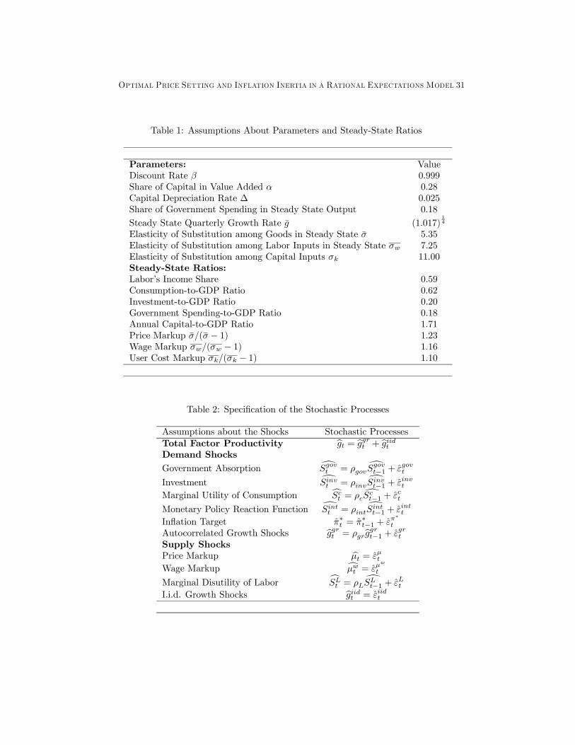
Optimal Price Setting and Inflation Inertia in a Rational Expectations Model 31
Table 1: Assumptions About Parameters and Steady-State Ratios
Parameters: ValueDiscount Rate β 0.999Share of Capital in Value Added α 0.28Capital Depreciation Rate ∆ 0.025Share of Government Spending in Steady State Output 0.18
Steady State Quarterly Growth Rate g (1.017)14
Elasticity of Substitution among Goods in Steady State σ 5.35Elasticity of Substitution among Labor Inputs in Steady State σw 7.25Elasticity of Substitution among Capital Inputs σk 11.00Steady-State Ratios:Labor’s Income Share 0.59Consumption-to-GDP Ratio 0.62Investment-to-GDP Ratio 0.20Government Spending-to-GDP Ratio 0.18Annual Capital-to-GDP Ratio 1.71Price Markup σ/(σ − 1) 1.23Wage Markup σw/(σw − 1) 1.16User Cost Markup σk/(σk − 1) 1.10
Table 2: Specification of the Stochastic Processes
Assumptions about the Shocks Stochastic ProcessesTotal Factor Productivity bgt = bggrt + bgiidtDemand ShocksGovernment Absorption dSgovt = ρgov
dSgovt−1 + εgovt
Investment dSinvt = ρinvdSinvt−1 + εinvt
Marginal Utility of Consumption cSct = ρc dSct−1 + εctMonetary Policy Reaction Function dSintt = ρint
dSintt−1 + εintt
Inflation Target π∗t = π∗t−1 + επ∗
t
Autocorrelated Growth Shocks bggrt = ρgrbggrt−1 + εgrtSupply ShocksPrice Markup bµt = εµtWage Markup cµwt = εµ
w
t
Marginal Disutility of Labor cSLt = ρLdSLt−1 + εLt
I.i.d. Growth Shocks bgiidt = εiidt

Optimal Price Setting and Inflation Inertia in a Rational Expectations Model 32
Table 3: Estimation ResultsParameters
Prior Mean Estimate 90% Interval Density Std
v 0.85 0.90 0.84-0.97 Beta 0.10γ 0.50 0.55 0.41-0.69 Normal 0.10δ 0.66 0.74 0.69-0.78 Beta 0.10δw 0.66 0.55 0.44-0.67 Beta 0.10δk 0.66 0.66 0.50-0.82 Beta 0.10φ 1.00 1.03 0.71-1.34 Normal 0.20φw 1.00 1.00 0.68-1.29 Normal 0.20φk 1.00 1.00 0.68-1.33 Normal 0.20θk 5.00 4.97 3.32-6.69 Normal 1.00θi 50.00 63.87 51.2-77.1 Normal 10.00ξint 0.50 0.85 0.73-0.96 Normal 0.20ξπ 0.50 0.43 0.23-0.62 Normal 0.20
Table 4: Estimation Results ContinuedParameters
Prior Estimate 90% Interval Density Std
ρgov 0.85 0.99 0.98-1.00 Beta 0.10ρinv 0.85 0.71 0.55-0.88 Beta 0.10ρc 0.85 0.75 0.59-0.92 Beta 0.10
ρint 0.85 0.75 0.65-0.86 Beta 0.10ρgr 0.95 0.95 0.93-0.97 Beta 0.01ρL 0.85 0.87 0.74-1.00 Beta 0.10

Optimal Price Setting and Inflation Inertia in a Rational Expectations Model 33
Table 5: Estimation Results ContinuedStandard Deviation of Shocks
Prior Estimate 90% Interval Density std
σεgov 0.025 0.0156 0.0133-0.0180 invg infσεinv 0.2000 0.0638 0.0498-0.0787 invg infσεc 0.0250 0.0631 0.0238-0.1029 invg infσεint 0.0100 0.0036 0.0030-0.0042 invg infσεπ∗ 0.1000 0.0205 0.0173-0.0236 invg infσεiid 0.0010 0.0064 0.0053-0.0073 invg infσεgr 0.2000 0.0948 0.0498-0.1358 invg infσεL 0.0050 0.0062 0.0011-0.0115 invg infσεµ 0.0250 0.0404 0.0288-0.0500 invg infσεµw 0.0250 0.1328 0.0749-0.1942 invg inf
Table 6: Contributions of Shocks to Future Level Changes in Output (N QuartersAhead
Quarters Ahead 1 4 20 40 100
Demand Shocksσεgr 10.6 17.2 43.2 61.7 69.5σεgov 0.46 0.65 0.45 0.41 0.67σεinv 44.8 37.0 26.9 19.7 16.8σεc 16.4 15.5 12.8 7.5 4.8σεint 17.2 16.3 6.0 3.3 2.3σεπ∗ 0.8 0.85 0.56 0.37 0.29
Demand Shocks Sum 93.2 92.2 97.3 98.1 98.6
Supply Shocksσεiid 5.1 6.0 1.7 1.2 0.9σεL 0.04 0.06 0.05 0.06 0.05σεµ 0.9 0.8 0.4 0.3 0.2σεµw 2.0 2.3 0.6 0.3 0.2
Supply Shocks Sum 6.8 7.8 2.7 1.9 1.4

Optimal Price Setting and Inflation Inertia in a Rational Expectations Model 34
Table 7: Comparison of Marginal Likelihoods with BVARs
Marginal Likelihood
Base Case Model (Laplace Approximation) -687.12Base Case Model (MH Replications = 150,000) -686.41
BVAR (1 lag) -734.16BVAR (2 lag) -736.50BVAR (3 lag) -733.16BVAR (4 lag) -725.07BVAR (5 lag) -725.61BVAR (6 lag) -728.81BVAR (7 lag) -730.00BVAR (8 lag) -733.92
Table 8: Comparison of the base-case DSGE model with DSGE models estimatedwith different assumptions
Marginal Likelihood
Base-Case Model -686.4No sticky user costs (φk=0, δk = 0.001) -687.9No upward-sloping MC curve (φ = φw = φk = 0) -705.3No sticky user costs, no upward-sloping MC curve -704.3
Calvo Model, Base-Case -687.6Calvo Model, No sticky user costs -691.8Calvo Model, No upward-sloping MC curve -689.6Calvo Model, No sticky user costs, no. upward-sloping, -690.5

Optimal Price Setting and Inflation Inertia in a Rational Expectations Model 35
Figure 1: Measures of Long-Term Inflation Expectations and Interest Rates
1990 1992 1994 1996 1998 2000 2002 20042
3
4
5
6
7
8
9
2
3
4
5
6
7
8
9
Consensus Forecast Inflation ForecastSurvey of Professional Forecasters Inflation ForecastLivingston Inflation ForecastLong-Term Nominal Interest Rate

Optimal Price Setting and Inflation Inertia in a Rational Expectations Model 36
Figure 2: Measures of Expected Long-Term Growth
1990 1992 1994 1996 1998 2000 2002 2004-2
-1
0
1
2
3
4
5
-2
-1
0
1
2
3
4
5
GDP GrowthConsensus Forecast GDP Growth ForecastSurvey of Professional Forecasters GDP Growth ForecastLivingston GDP Growth Forecast

Optimal Price Setting and Inflation Inertia in a Rational Expectations Model 37
Figure 3: Shock to the Fed Funds Rate (Demand)
10 20 30 40−0.8
−0.6
−0.4
−0.2
0GDP
10 20 30 40−0.6
−0.4
−0.2
0
0.2Consumption
10 20 30 40−2
−1
0
1Investment
10 20 30 40−1
−0.5
0Real Wage
10 20 30 40−0.2
−0.1
0Output per Hour
10 20 30 40−0.5
0
0.5YoY Inflation
10 20 30 40−0.2
0
0.2
0.4
0.6Interest Rate
10 20 30 40−0.5
0
0.5
1Real Interest Rate
10 20 30 40−0.6
−0.4
−0.2
0
0.2Hours Worked

Optimal Price Setting and Inflation Inertia in a Rational Expectations Model 38
Figure 4: Shock to the Inflation Objective (Demand)
10 20 30 400
0.05
0.1
0.15
0.2GDP
10 20 30 400
0.05
0.1Consumption
10 20 30 400
0.1
0.2
0.3
0.4Investment
10 20 30 400
0.1
0.2Real Wage
10 20 30 400
0.01
0.02
0.03Output per Hour
10 20 30 40−0.1
0
0.1YoY Inflation
10 20 30 40−0.1
0
0.1
0.2
0.3Interest Rate
10 20 30 40−0.15
−0.1
−0.05
0
0.05Real Interest Rate
10 20 30 40−0.05
0
0.05
0.1
0.15Hours Worked

Optimal Price Setting and Inflation Inertia in a Rational Expectations Model 39
Figure 5: Shock to Consumption (Demand)
10 20 30 40−0.2
0
0.2
0.4
0.6GDP
10 20 30 40−0.5
0
0.5
1
1.5Consumption
10 20 30 40−1.5
−1
−0.5
0Investment
10 20 30 40−0.2
0
0.2Real Wage
10 20 30 40−0.05
0
0.05Output per Hour
10 20 30 40−0.1
0
0.1YoY Inflation
10 20 30 40−0.1
0
0.1
0.2
0.3Interest Rate
10 20 30 40−0.1
0
0.1
0.2
0.3Real Interest Rate
10 20 30 40−0.2
0
0.2
0.4
0.6Hours Worked

Optimal Price Setting and Inflation Inertia in a Rational Expectations Model 40
Figure 6: Shock to Wage Markup (Supply)
10 20 30 400
0.05
0.1
0.15
0.2GDP
10 20 30 40−0.05
0
0.05
0.1
0.15Consumption
10 20 30 40−0.2
0
0.2
0.4
0.6Investment
10 20 30 40−1
−0.5
0
0.5Real Wage
10 20 30 40−0.2
0
0.2Output per Hour
10 20 30 40−0.1
0
0.1YoY Inflation
10 20 30 40−0.15
−0.1
−0.05
0
0.05Interest Rate
10 20 30 40−0.2
−0.1
0
0.1
0.2Real Interest Rate
10 20 30 40−0.1
0
0.1
0.2
0.3Hours Worked

Optimal Price Setting and Inflation Inertia in a Rational Expectations Model 41
Figure 7: Shock to Price Markup (Supply)
10 20 30 400
0.05
0.1
0.15
0.2GDP
10 20 30 40−0.05
0
0.05
0.1
0.15Consumption
10 20 30 400
0.1
0.2
0.3
0.4Investment
10 20 30 400
0.1
0.2Real Wage
10 20 30 400
0.02
0.04
0.06Output per Hour
10 20 30 40−0.2
0
0.2YoY Inflation
10 20 30 40−0.3
−0.2
−0.1
0
0.1Interest Rate
10 20 30 40−0.3
−0.2
−0.1
0
0.1Real Interest Rate
10 20 30 40−0.05
0
0.05
0.1
0.15Hours Worked

Optimal Price Setting and Inflation Inertia in a Rational Expectations Model 42
Figure 8: Shock to Productivity Level (Supply)
10 20 30 400
0.2
0.4
0.6
0.8GDP
10 20 30 400
0.2
0.4
0.6
0.8Consumption
10 20 30 400
0.5
1Investment
10 20 30 400
0.5
1Real Wage
10 20 30 400
0.5
1Output per Hour
10 20 30 40−0.1
0
0.1YoY Inflation
10 20 30 40−0.15
−0.1
−0.05
0
0.05Interest Rate
10 20 30 40−0.2
−0.1
0
0.1
0.2Real Interest Rate
10 20 30 40−0.3
−0.2
−0.1
0
0.1Hours Worked

Optimal Price Setting and Inflation Inertia in a Rational Expectations Model 43
Figure 9: Shock to Productivity Growth (Demand)
10 20 30 400
0.5
1
1.5GDP
10 20 30 400
0.5
1
1.5Consumption
10 20 30 40−0.5
0
0.5
1Investment
10 20 30 400
0.5
1
1.5Real Wage
10 20 30 400
0.5
1
1.5Output per Hour
10 20 30 40−0.05
0
0.05YoY Inflation
10 20 30 40−0.05
0
0.05
0.1
0.15Interest Rate
10 20 30 40−0.05
0
0.05
0.1
0.15Real Interest Rate
10 20 30 40−0.15
−0.1
−0.05
0
0.05Hours Worked

Optimal Price Setting and Inflation Inertia in a Rational Expectations Model 44
Figure 10: Inflation Target Shock and Inflation Dynamics
0 10 20 300
1
2 delta=0.25 , phi=0.5
0 10 20 300
1
2 delta=0.25 , phi=1
0 10 20 300
1
2 delta=0.25 , phi=2
0 10 20 300
1
2 delta=0.25 , phi=5
0 10 20 300
1
2 delta=0.5 , phi=0.5
0 10 20 300
1
2 delta=0.5 , phi=1
0 10 20 300
1
2 delta=0.5 , phi=2
0 10 20 300
1
2 delta=0.5 , phi=5
0 10 20 300
1
2 delta=0.75 , phi=0.5
0 10 20 300
1
2 delta=0.75 , phi=1
0 10 20 300
1
2 delta=0.75 , phi=2
0 10 20 300
1
2 delta=0.75 , phi=5
0 10 20 300
1
2 delta=0.9 , phi=0.5
0 10 20 300
1
2 delta=0.9 , phi=1
0 10 20 300
1
2 delta=0.9 , phi=2
0 10 20 300
1
2 delta=0.9 , phi=5

Optimal Price Setting and Inflation Inertia in a Rational Expectations Model 45
Figure 11: Estimated Structural Shocks
20 40 60−0.2
−0.1
0
0.1
0.2E_C
20 40 60−0.02
−0.01
0
0.01
0.02E_GIID
20 40 60−0.04
−0.02
0
0.02
0.04E_GOV
20 40 60−0.1
−0.05
0
0.05
0.1E_GROWTH
20 40 60−0.02
−0.01
0
0.01E_INT
20 40 60−0.2
−0.1
0
0.1
0.2E_INV
20 40 60−4
−2
0
2x 10
−4 E_L
20 40 60−0.2
−0.1
0
0.1
0.2E_MU
20 40 60−0.4
−0.2
0
0.2
0.4E_MUW

Optimal Price Setting and Inflation Inertia in a Rational Expectations Model 46
Figure 12: Estimated Inflation Objectives
0 10 20 30 40 50 60 702
2.5
3
3.5
4
4.5