Embed Size (px)
Citation preview
OPTIMAL PROCUREMENT POLICY FOR
COST CONSCIOUS RETAILER
By SICONG HOU
A thesis submitted to the
Graduate School-New Brunswick
Rutgers, The State University of New Jersey
in partial fulfillment of the requirements
for the degree of
Master of Science
Graduate Program in
Operations Research
Written under the direction of
Professor Melike Baykal-Gürsoy
and approved by
________________________
________________________
________________________
New Brunswick, New Jersey
May, 2013
ii
ABSTRACT OF THE THESIS
OPTIMAL PROCUREMENT POLICY FOR
COST CONSCIOUS RETAILER
By SICONG HOU
Thesis Director:
Professor Melike Baykal-Gürsoy
Manufacturers whose products primarily relay on expensive raw materials
need to make well informed procurement decisions in order to reduce their
production costs. Decision making is especially difficult when there is uncertainty
about the raw material cost as well as the product demand. This research considers
an optimum procurement and production planning problem under uncertainty.
Basic raw material is a rare metal with a dynamically and stochastically changing
price. The manufacturer has the dual sourcing option: buy from the spot market; or
to sign long term contracts. Long term contracts can be signed only at the beginning
of every year with a yearly duration. In addition, the contract price depends on the
average spot price during some interval. We first consider a simplified version of the
problem without long-term contract, and assume a base-stock procurement and
inventory control policy. We model the problem as a Markov chain and present
some numerical examples demonstrating the effect of various parameters on the
optimum base-stock value. Then, we investigate a case with dual procurement
option, and present our results.

iii
ACKNOWLEDGEMENT
It is with immense gratitude that I acknowledge the support and help of my
thesis advisor Dr. Melike Baykal-Gürsoy, who continually and convincingly
conveyed a spirit of adventure in regard to research and scholarship, without her
continuous guidance and persistent help this thesis would not have been possible.
I would like to express my appreciation to my committee member and my
program director Dr. Endre Boros for his support and encouragement during the
research.
I would also like to thank Dr. András Prékopa for serving on my thesis
committee and giving me valuable suggestions.
In addition, I take the opportunity to thank Mr. Bora and Mr. Figueroa as well
as all graduate students of Rutgers Center for Operations Research for their support
and help.

iv
DEDICATION
This thesis is dedicated to my parents who have given me the opportunity of
an education from the best institutions and support throughout my life. They have
always stood by me and gave me the strength to carry out my studies.
v
Table of Contents
Abstract .......................................................................................................................................................... ii
Acknowledgements .................................................................................................................................. iii
Dedication .................................................................................................................................................... iv
List of Tables .............................................................................................................................................. vii
List of Figures ...........................................................................................................................................viii
1. Introduction ............................................................................................................................................ 1
2. Literature Review ................................................................................................................................. 3
3. A simplified Markov Chain Model of the Inventory/Production Control of a Cost
Conscious Retailer ..................................................................................................................................... 7
3.1 Assumptions and Notations ...................................................................................................... 7
3.2 Model Description ......................................................................................................................... 9
3.3 Optimization .................................................................................................................................. 17
3.4 Numerical Results ........................................................................................................................ 19
4. A Case Study ......................................................................................................................................... 30
4.1 Introduction ................................................................................................................................... 30
4.2 Data Preparation and Forecasting ........................................................................................ 32
vi
4.3 Modeling .......................................................................................................................................... 46
4.4 Optimization Result .................................................................................................................... 48
5. Conclusions ............................................................................................................................................ 51
Appendix A.................................................................................................................................................. 52
Appendix B .................................................................................................................................................. 55
References ................................................................................................................................................... 59
vii
List of Tables
3.1. Price Inventory transition probability matrix ...................................................................... 8
3.2. Price Inventory transition probability matrix for K=2 .................................................. 12
3.3. Price Inventory transition probability matrix for K=3 .................................................. 12
3.4. Price Inventory transition probability matrix for K=4 .................................................. 13
3.5. Price Inventory transition probability matrix for K=5 and K=6 ............................... 14
3.6. Price Inventory transition probability matrix for 𝐊 ≥ 𝟔 ............................................... 15
3.7. Effect of 𝛑𝐇 and 𝐘𝐇 on K* ............................................................................................................. 20
3.8. Effect of 𝛑𝐇 and 1-p on K* ........................................................................................................... 22
3.9. Effect of 𝛑𝐇 and h on K* ................................................................................................................ 23
3.10: Effect of 1-p and 𝐘𝐇 on K* ......................................................................................................... 25
3.11. Effect of h and 𝐘𝐇 on K* .............................................................................................................. 26
3.12. Effect of h and 1-p on K* ............................................................................................................ 28
3.13. Effect of 𝛑𝐇, 𝐘𝐇, h and p on K* ................................................................................................. 29
4.1. Predicted price from SPSS “autoarima” ................................................................................. 45
4.2: Predicted demand from SPSS “autoarima” .......................................................................... 45
viii
List of Figures
3.1. Visualization of the dependence of K* on 𝛑𝐇 and 𝐘𝐇 ....................................................... 21
3.2. Visualization of the dependence of K* on 𝛑𝐇 and 1-p .................................................... 22
3.3. Visualization of the dependence of K* on 𝛑𝐇 and h ........................................................ 24
3.4. Visualization of the dependence of K* on 1-p and 𝐘𝐇 ...................................................... 25
3.5. Visualization of the dependence of K* on h and 𝐘𝐇 .......................................................... 27
3.6. Visualization of the dependence of K* on h and 1-p ....................................................... 28
4.1. Weekly historical data of spot prices ...................................................................................... 33
4.2. AC and PAC plots of original data ............................................................................................. 34
4.3. 1-differenced and mean subtracted data of spot prices ................................................. 36
4.4. AC and PAC plots of 1-differenced and mean subtracted data .................................... 37
4.5. SPSS “autoarima” fit and forecast ............................................................................................ 40
4.6. Eviews ARMA(1,1) fit and forecast ........................................................................................ 41
4.7. Excel ARMA(3,1) fit and forecast ............................................................................................ 42
4.8. R GARCH fit and forecast ............................................................................................................. 43
1
Chapter 1
Introduction
Procurement problems, particularly direct procurement problems
concerning mainly raw material and production goods, are becoming more and
more prominent in supply chain management these days because they greatly affect
the total expenditure of many companies. This is especially true when the raw
material is an expensive rare metal. This research considers an optimum
procurement and production planning problem under raw material price and
demand uncertainty. The raw material used to produce an intermediate product is a
rare metal with dynamically and stochastically changing prices. The demand for the
intermediate product is also random but reasonably stationary.
The manufacturer has dual sourcing options; they can either buy from the
spot market, or sign a long term forward contract. That is, dual sourcing is
comprised of forward contract buying and spot market buying. Forward contract
buying provides a long term stable supply at a fixed price for a fixed delivery time.
While spot buying, although is more flexible with the delivery times and the order
quantity, is more risky and uncertain. For instance, you might not able to purchase a
large volume when the price is good because other companies already took the
advantage first. According to Zhang et al. (2011), in recent years spot markets have
emerged for a wide variety of commodities, and companies are starting to use it to
2
incorporate with the traditional forward contracts especially in dynamic random
access memory procurements. The market has been a mix of private, bilateral
contracts and spot market trading for years, where 80% of the intermediate
products are sold through a fixed price long term contract.
For large manufacturers, especially in chemical and pharmaceutical
industries whose products primarily relay on expensive raw materials, their
production costs can be largely reduced if good strategies be adopted when making
procurement decisions. However, these complex strategies of decision making are
very difficult considering the demand uncertainty and randomness of the raw
material costs. Most of the mathematical models fail to predict a jump or slump on
the prices because sudden events that cause such a jump or slump to happen are
impossible to predict sometimes. Relatively, the demand of products is also
uncertain but may be easier to predict since we have a more stable requirement for
the materials globally. Thus the strategy that is applied in order to compensate the
possible failure of forecasting raw material price becomes very important for the
dual sourcing scenario.
In Chapter 2, we present the literature survey. Chapter 3 considers a
simplified model of the procedure for a problem without long term contract. The
effect of various parameters on the optimum order quality is investigated. A case in
which both long term contract and spot buying are available is studied in Chapter 4
with real world data and situations. Finally, in Chapter 5, conclusions and future
research are discussed.
3
Chapter 2
Literature Review
Many optimization approaches based on periodic updates have been used in
commodity procurement. Secomandi and Kekre (2009) consider the problem of
reselling the commodity back to the market in the forward process. They suggest
not only to update the forward price, but also to update the demand forecast. Thus
the whole dynamic optimization can provide a better solution overall. Optimal cost
value function is provided through a Markov decision process formulation.
For a typical periodic-review inventory control model with stochastic
demand, Goel and Gutierrez (2012) characterized the optimal procurement policy
and developed a computational algorithm to obtain the optimal policy thresholds.
The model they developed has a total cost consists of procurement cost and a
market-determined economic cost of holding inventory, and this economic cost can
be significantly reduced according to the numerical results from this paper. Also
they considered a dynamic program with a risk-neutral valuation approach for
minimizing the total procurement cost.
In comparing the forward contract with the total order quantity commitment,
the latter is more flexible according to the paper of Zhang, Chen, Hua and Xue
(2011). Hence, it is easier to use it and take advantage of the dual sourcing. In this
4
paper they suppose a stochastic demand and the spot price can be stationary or
non-stationary, but it is independent of the demand process.
Two of the papers focused on a dual sourcing scenario of periodic-review
inventory model. First one by Inderfurth, Kelle and Kleber (2013) assume random
stationary demand and a capacity reservation contract for the sourcing. In this
modeling part, they used dynamic programming recursive equations. However,
when formulating the models, this paper focuses more on the structure analysis,
because of the special reservation capacity decision needed to be considered. The
model can be extended to be optimal for infinite horizon, too. A heuristic approach
is used for determining iterative parameters step by step. The second one by Seifert,
Thonemann and Hausman (2004) mentioned that in these problems the demand
and the spot price are usually positively correlated, and thus assume a bivariate
distribution rather than a normal distribution. Their paper then deals with dynamic
pricing and determines the contract-to-spot ratio for purchases, where in spot
market we need to consider a hedging situation since it allows salvage. Based on the
assumed distribution, we can adjust the multiplier of the deviation to set different
policies for different level of risks you wish to take. Also, a spot price premium case
was studied, as well as a pure contract sourcing case.
Other two papers focused on a multi-period model with a single product.
Nagarajan and Rajagopalan (2009) first consider a comprehensive environment and
the equilibrium order quantities have the special property such that each player
ignores the strategy of his opponent under reasonable conditions on the cost
5
parameters. Secondly, they show that under certain conditions, the equilibrium
quantities in the finite horizon game can be reduced to a multi-period single-
product inventory model for each player. Then they approach to the equilibrium by
proving the deterministic demand identifies a unique Nash equilibrium while
stochastic demand derived from a decoupling result. Thus, the equilibrium
strategies of two players is simply to solve a single-product in n-period stochastic
inventory model with partial backlogging instead of lost sales, where the demand of
non-substituting customers from the current period is back logged to the next
period.
Hwang and Hahn (2000) studied a periodic review inventory model for a
single perishable product and demand rate of the item is dependent on the current
inventory level. The proof first shows some properties about the ordering quantity.
Since the item have a fixed life time, two different kind of order up to values are
introduced depending on the outdated items. They approach to solve the two
different situations by using linear programming and then apply enumeration
method which has a similar approach to dynamic programming.
The last optimal procurement policy paper we reviewed here by Polatoglu
and Sahin (2000), studied a (s,S) type inventory control model under price-
dependent demand relationship. The main difference in the model of this paper is
that the price is a decision variable here and brings two opposing cost-related
effects. The solution approach is also dynamic programming. However, an n-period
pseudo-profit function is introduced instead. And finally, the problem is solved by

6
investigating the critical inventory level of (s,S) under certain sufficient condition.
Some special situations such as No-fixed-ordering-cost, Non-stationary extensions
and deterministic demand are also considered in the end of this paper.
7
Chapter 3
A simplified Markov Chain Model of the Inventory/Production
Control of a Cost Conscious Retailer
In this section our goal is to build a Markov chain model for base-stock type
procurement policies, and then analyze the effects of various parameters on the
optimum order quantity. Dual sourcing will not be considered in this chapter but
will be discussed in detail in Chapter 4.
3.1 Assumptions and Notations
We begin modeling by making some necessary assumptions for the
inventory/production control policy. The procurement policy is adopted depending
on the price level and the inventory on hand. We assume the order of each month’s
operations are as follows: Production facility consumes items from the inventory to
meet demand, notice demand is always met here since we have the minimum
inventory level that is equal to the maximum daily demand. Then we observe the
current price level and the number of items in stock, in order to decide on how
many items to purchase. Lastly, after we finish the purchasing stage, we check our
new inventory level and set it as the next inventory level.
8
To simplify the problem, we assume only two price levels: H, denoting the
state of high price level, and L, denoting the state of low price level. The unit cost for
low price level is denoted as YL and for high price level is denoted as YH.
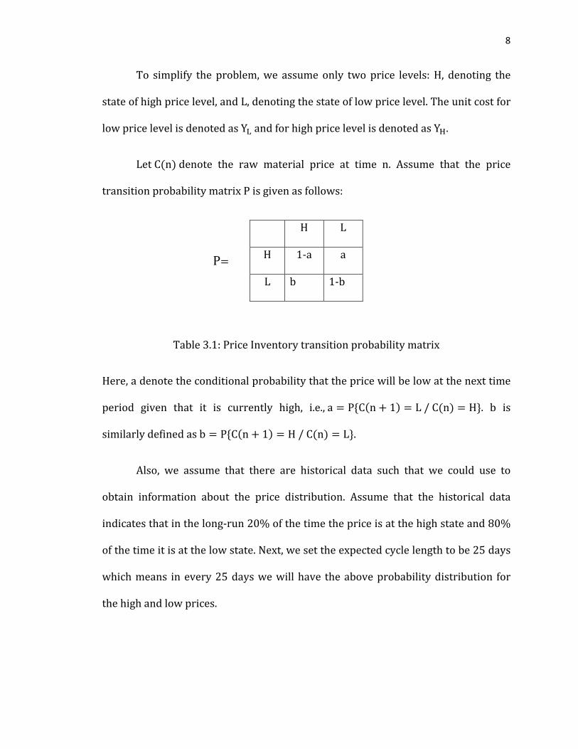
Let C(n) denote the raw material price at time n. Assume that the price
transition probability matrix P is given as follows:
H L
H 1-a a
L b 1-b
Table 3.1: Price Inventory transition probability matrix
Here, a denote the conditional probability that the price will be low at the next time
period given that it is currently high, i.e., a = P{C(n + 1) = L / C(n) = H}. b is
similarly defined as b = P{C(n + 1) = H / C(n) = L}.
Also, we assume that there are historical data such that we could use to
obtain information about the price distribution. Assume that the historical data
indicates that in the long-run 20% of the time the price is at the high state and 80%
of the time it is at the low state. Next, we set the expected cycle length to be 25 days
which means in every 25 days we will have the above probability distribution for
the high and low prices.
P=
9
We assume the demand for raw material is distributed in a very simplified
fashion; demand on day n is equal to 1 item with probability p and 2 items with
probability (1-p). That is, let Dn denote the demand quantity at time n, we have:
P{Dn = 1} = p, P{Dn = 2} = 1 − p
When the price is low, we purchase enough items to stock up to the
maximum inventory of K items. When the price is high, we do not purchase unless
the number of items we have on hand are less than the maximum daily demand.
More specifically, if the price level is high we only purchase when the inventory
level is below 2 and if so, we purchase to bring the inventory level back to the
minimum of 2 items.
Lastly, we assume that the total cost of inventory/production management
consists of the inventory holding cost and the procurement cost, where the holding
cost is $h/day per item and the procurement cost is the total cost of all the
purchases made.
3.2 Model Description
Now we are ready for the modeling of our inventory management
problems. The objective of our model is to optimize the inventory/production policy
we utilized, and therefore to minimize the expected total cost under such a policy.
Later on we will see that the expected total cost is decided by the base-stock value,
10
which is K. However, we would like to obtain the actual values of a and b before we
calculate the expected total cost and start the optimization.
Let πH and πL denote the stationary probability of price states H and L
respectively. In Table 3.1 matrix we can obtain all the transition probabilities
between the states by having the following relations:
�
πH = 0.2 and πL = 0.8a ≥ 0, b ≥ 0
[πH, πL] = [πH, πL] ∗ �1 − a ab 1 − b�
⟹ a = 4b ⋯ ⋯ ⋯ ⋯ ⋯ (1)
and a ≥ 0, b ≥ 0
Next, we use the fact that the cycle length is on the average of 25 days, where
20% of a cycle is at the high state, and 80% of a cycle is at the low state, in order to
calculate the exact a and b values. Let the first day be day 0 and since a cycle is 25
days, next cycle starts at day 25. Consider the probability that the first time a high
state goes to low state; it is exactly the probability for the number of consecutive
days that a high state stay at high, before it goes to low. The corresponding expected
values for the number of consecutive days at the high state before it goes to low is
exactly equal to the total number of days at high state.
P {X=n} = P {the first time H goes to L at day n} = (1 − a)n ∗ a
11
Let X denotes the number of consecutive days at H before it goes to L in one
cycle. Since we know that for a geometrically distributed random variable X, the
expected value is:
E(X) =1 − a
a
It means that the expected number of days at H is equal to 1−aa
as well.
Similarly, we can obtain the expected number of days at L is equal to 1−bb
. Now, we
also know that the expected cycle length is 25days, so:
1 − aa
+1 − b
b= 25 ⋯ ⋯ ⋯ ⋯ ⋯ (2)
We can then obtain a, b values by combining equations (1) and (2) above,
getting results for the price transition probability matrix:
a =20
108, b =
5108
Now we can start to build the detailed model of the inventory control
problem. We want to have this matrix because we can then use it to compute the
expected total cost which is ultimately what we intend to optimize. Let
{C(n)I(n)} n ≥ 0 denote the two-dimensional state, where C(n) is the price state and
I(n) is the inventory on hand at the beginning of nth time period. For example, Hm
denotes the state of high price level with inventory of m items, and similarly Lm
denotes the state of low price level with inventory of m items.
12
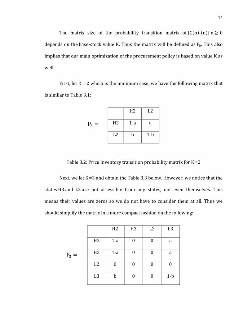
The matrix size of the probability transition matrix of {C(n)I(n)} n ≥ 0
depends on the base-stock value K. Thus the matrix will be defined as Pk This also .
implies that our main optimization of the procurement policy is based on value K as
well.
First, let K =2 which is the minimum case, we have the following matrix that
is similar to Table 3.1:
H2 L2
H2 1-a a
L2 b 1-b
Table 3.2: Price Inventory transition probability matrix for K=2
Next, we let K=3 and obtain the Table 3.3 below. However, we notice that the
states H3 and L2 are not accessible from any states, not even themselves. This
means their values are zeros so we do not have to consider them at all. Thus we
should simplify the matrix in a more compact fashion on the following:
H2 H3 L2 L3
H2 1-a 0 0 a
H3 1-a 0 0 a
L2 0 0 0 0
L3 b 0 0 1-b
P2 =
P3 =
13
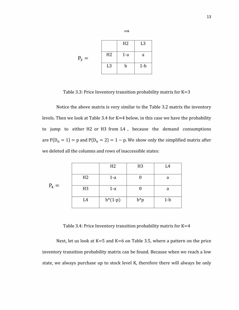
⟹
H2 L3
H2 1-a a
L3 b 1-b
Table 3.3: Price Inventory transition probability matrix for K=3
Notice the above matrix is very similar to the Table 3.2 matrix the inventory
levels. Then we look at Table 3.4 for K=4 below, in this case we have the probability
to jump to either H2 or H3 from L4 , because the demand consumptions
are P{Dn = 1} = p and P{Dn = 2} = 1 − p. We show only the simplified matrix after
we deleted all the columns and rows of inaccessible states:
H2 H3 L4
H2 1-a 0 a
H3 1-a 0 a
L4 b*(1-p) b*p 1-b
Table 3.4: Price Inventory transition probability matrix for K=4
Next, let us look at K=5 and K=6 on Table 3.5, where a pattern on the price
inventory transition probability matrix can be found. Because when we reach a low
state, we always purchase up to stock level K, therefore there will always be only
P3 =
P4 =
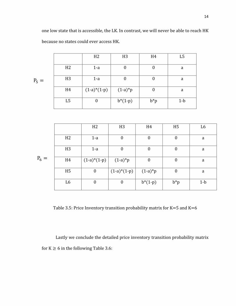
14
one low state that is accessible, the LK. In contrast, we will never be able to reach HK
because no states could ever access HK.
H2 H3 H4 L5
H2 1-a 0 0 a
H3 1-a 0 0 a
H4 (1-a)*(1-p) (1-a)*p 0 a
L5 0 b*(1-p) b*p 1-b
H2 H3 H4 H5 L6
H2 1-a 0 0 0 a
H3 1-a 0 0 0 a
H4 (1-a)*(1-p) (1-a)*p 0 0 a
H5 0 (1-a)*(1-p) (1-a)*p 0 a
L6 0 0 b*(1-p) b*p 1-b
Table 3.5: Price Inventory transition probability matrix for K=5 and K=6
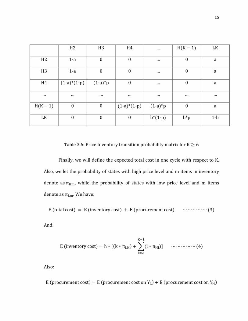
Lastly we conclude the detailed price inventory transition probability matrix
for K ≥ 6 in the following Table 3.6:
P6 =
P5 =
15
H2 H3 H4 … H(K − 1) LK
H2 1-a 0 0 … 0 a
H3 1-a 0 0 … 0 a
H4 (1-a)*(1-p) (1-a)*p 0 … 0 a
… … … … … … …
H(K − 1) 0 0 (1-a)*(1-p) (1-a)*p 0 a
LK 0 0 0 b*(1-p) b*p 1-b
Table 3.6: Price Inventory transition probability matrix for K ≥ 6
Finally, we will define the expected total cost in one cycle with respect to K.
Also, we let the probability of states with high price level and m items in inventory
denote as πHm, while the probability of states with low price level and m items
denote as πLm. We have:
E (total cost) = E (inventory cost) + E (procurement cost) ⋯ ⋯ ⋯ ⋯ ⋯ (3)
And:
E (inventory cost) = h ∗ [(k ∗ πLK) + �(i ∗ πHi
K−1
i=2
)] ⋯ ⋯ ⋯ ⋯ ⋯ (4)
Also:
E (procurement cost) = E (procurement cost on YL) + E (procurement cost on YH)
16
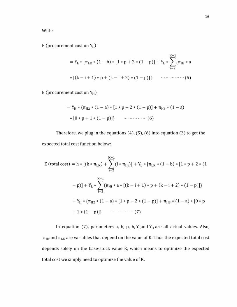
With:
E (procurement cost on YL)
= YL ∗ [πLK ∗ (1 − b) ∗ [1 ∗ p + 2 ∗ (1 − p)] + YL ∗ �{πHi
K−1
i=2
∗ a
∗ [(k − i + 1) ∗ p + (k − i + 2) ∗ (1 − p)]} ⋯ ⋯ ⋯ ⋯ ⋯ (5)
E (procurement cost on YH)
= YH ∗ {πH2 ∗ (1 − a) ∗ [1 ∗ p + 2 ∗ (1 − p)] + πH3 ∗ (1 − a)
∗ [0 ∗ p + 1 ∗ (1 − p)]} ⋯ ⋯ ⋯ ⋯ ⋯ (6)
Therefore, we plug in the equations (4), (5), (6) into equation (3) to get the
expected total cost function below:
E (total cost) = h ∗ [(k ∗ πLK) + �(i ∗ πHi
K−1
i=2
)] + YL ∗ [πLK ∗ (1 − b) ∗ [1 ∗ p + 2 ∗ (1
− p)] + YL ∗ �{πHi
K−1
i=2
∗ a ∗ [(k − i + 1) ∗ p + (k − i + 2) ∗ (1 − p)]}
+ YH ∗ {πH2 ∗ (1 − a) ∗ [1 ∗ p + 2 ∗ (1 − p)] + πH3 ∗ (1 − a) ∗ [0 ∗ p
+ 1 ∗ (1 − p)]} ⋯ ⋯ ⋯ ⋯ ⋯ (7)
In equation (7), parameters a, b, p, h, YLand YH are all actual values. Also,
πHiand πLK are variables that depend on the value of K. Thus the expected total cost
depends solely on the base-stock value K, which means to optimize the expected
total cost we simply need to optimize the value of K.
17
3.3 Optimization
After obtaining the expected total cost function, we will begin this section
with the minimization of the expected total cost and solve the optimal
inventory/production management problem with respect to K. That is, we will be
able to optimize our procurement policy if we can find the optimal value of the base-
stock value K*.
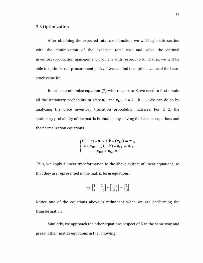
In order to minimize equation (7) with respect to K, we need to first obtain
all the stationary probability of state πHi and πLK, i = 2 … k − 1. We can do so by
analyzing the price inventory transition probability matrices. For K=2, the
stationary probability of the matrix is obtained by solving the balance equations and
the normalization equations.
�(1 − a) ∗ πH2 + b ∗ (πL2) = πH2
a ∗ πH2 + (1 − b) ∗ πL2 = πL2πH2 + πL2 = 1
Thus, we apply a linear transformation to the above system of linear equations, so
that they are represented in the matrix form equations:
⟹ �1 1a −b� ∗ �
πH2πL2
� = �10�
Notice one of the equations above is redundant when we are performing the
transformation.
Similarly, we approach the other equations respect of K in the same way and
present their matrix equations in the following:
18
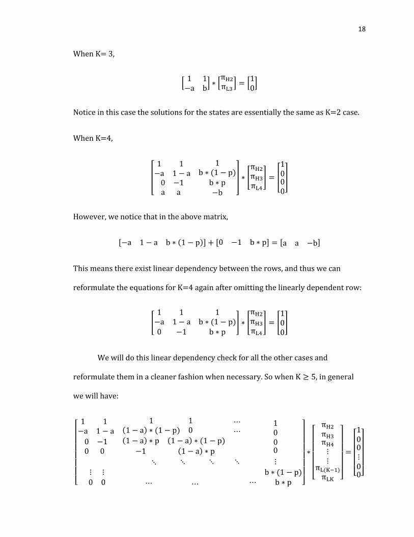
When K= 3,
� 1 1−a b� ∗ �
πH2πL3
� = �10�
Notice in this case the solutions for the states are essentially the same as K=2 case.
When K=4,
�
1 1−a 1 − a
1b ∗ (1 − p)
0 −1a a
b ∗ p−b
� ∗ �πH2πH3πL4
� = �1000
�
However, we notice that in the above matrix,
[−a 1 − a b ∗ (1 − p)] + [0 −1 b ∗ p] = [a a −b]
This means there exist linear dependency between the rows, and thus we can
reformulate the equations for K=4 again after omitting the linearly dependent row:
�1 1 1
−a 1 − a b ∗ (1 − p)0 −1 b ∗ p
� ∗ �πH2πH3πL4
� = �100
�
We will do this linear dependency check for all the other cases and
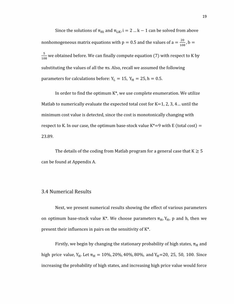
reformulate them in a cleaner fashion when necessary. So when K ≥ 5, in general
we will have:
⎣⎢⎢⎢⎢⎢⎢⎡ 1 1−a 1 − a
1 1(1 − a) ∗ (1 − p) 0
0 −10 0
(1 − a) ∗ p (1 − a) ∗ (1 − p)−1 (1 − a) ∗ p
⋯⋯
1000
⋱ ⋱ ⋱ ⋱ ⋮⋮ ⋮0 0 ⋯ ⋯
b ∗ (1 − p)⋯ b ∗ p ⎦
⎥⎥⎥⎥⎥⎥⎤
∗
⎣⎢⎢⎢⎢⎡
πH2πH3πH4
⋮⋮
πL(K−1)πLK ⎦
⎥⎥⎥⎥⎤
=
⎣⎢⎢⎢⎢⎡100⋮00⎦
⎥⎥⎥⎥⎤
19
Since the solutions of πHi and πLK, i = 2 … k − 1 can be solved from above
nonhomogeneous matrix equations with p = 0.5 and the values of a = 20108
, b =
5108
we obtained before. We can finally compute equation (7) with respect to K by
substituting the values of all the πs. Also, recall we assumed the following
parameters for calculations before: YL = 15, YH = 25, h = 0.5.
In order to find the optimum K*, we use complete enumeration. We utilize
Matlab to numerically evaluate the expected total cost for K=1, 2, 3, 4… until the
minimum cost value is detected, since the cost is monotonically changing with
respect to K. In our case, the optimum base-stock value K*=9 with E (total cost) =
23.89.
The details of the coding from Matlab program for a general case that K ≥ 5
can be found at Appendix A.
3.4 Numerical Results
Next, we present numerical results showing the effect of various parameters
on optimum base-stock value K*. We choose parameters πH, YH, p and h, then we
present their influences in pairs on the sensitivity of K*.
Firstly, we begin by changing the stationary probability of high states, πH and
high price value, YH. Let πH = 10%, 20%, 40%, 80%, and YH=20, 25, 50, 100. Since
increasing the probability of high states, and increasing high price value would force
20
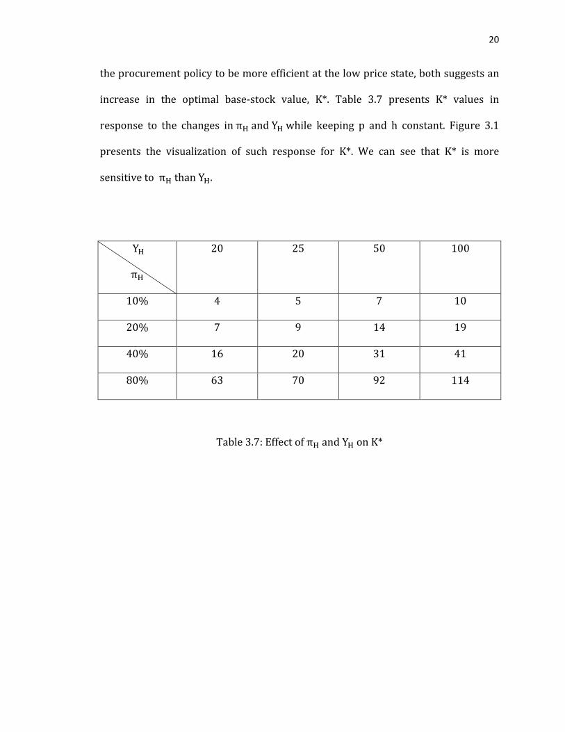
the procurement policy to be more efficient at the low price state, both suggests an
increase in the optimal base-stock value, K*. Table 3.7 presents K* values in
response to the changes in πH and YH while keeping p and h constant. Figure 3.1
presents the visualization of such response for K*. We can see that K* is more
sensitive to πH than YH.
YH
πH
20 25 50 100
10% 4 5 7 10
20% 7 9 14 19
40% 16 20 31 41
80% 63 70 92 114
Table 3.7: Effect of πH and YH on K*
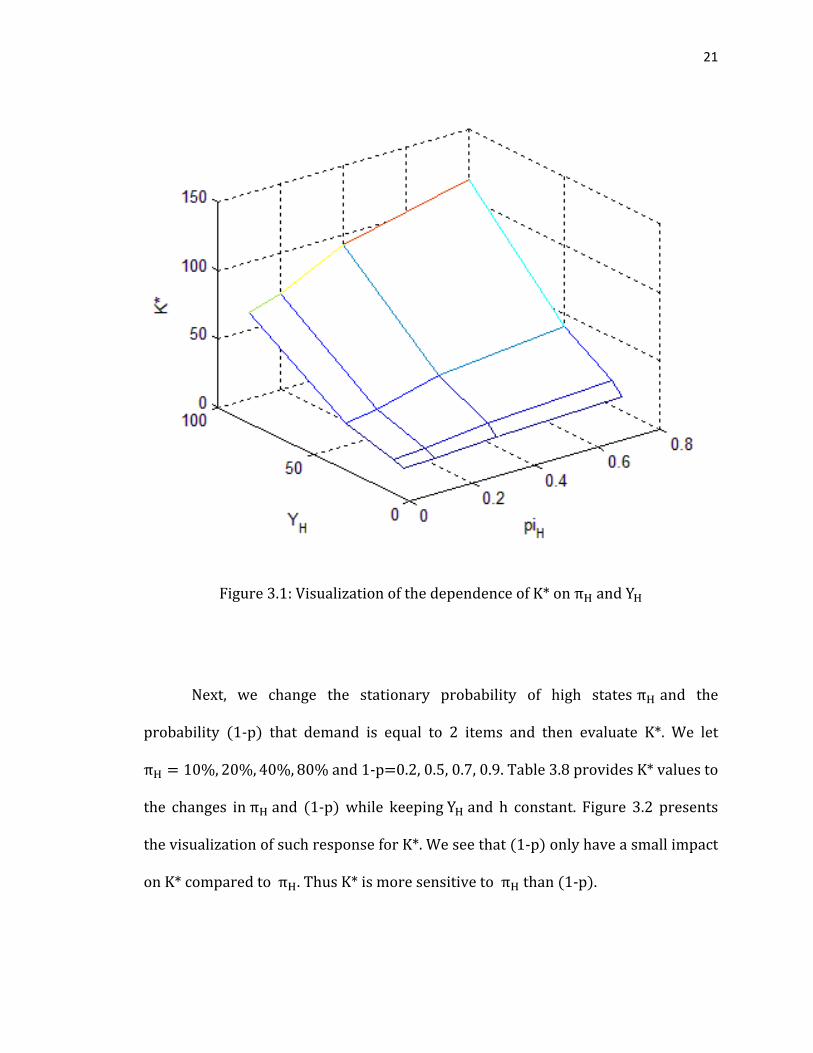
21
Figure 3.1: Visualization of the dependence of K* on πH and YH
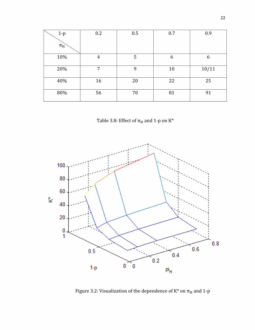
Next, we change the stationary probability of high states πH and the
probability (1-p) that demand is equal to 2 items and then evaluate K*. We let
πH = 10%, 20%, 40%, 80% and 1-p=0.2, 0.5, 0.7, 0.9. Table 3.8 provides K* values to
the changes in πH and (1-p) while keeping YH and h constant. Figure 3.2 presents
the visualization of such response for K*. We see that (1-p) only have a small impact
on K* compared to πH. Thus K* is more sensitive to πH than (1-p).
22
1-p
πH
0.2 0.5 0.7 0.9
10% 4 5 6 6
20% 7 9 10 10/11
40% 16 20 22 25
80% 56 70 81 91
Table 3.8: Effect of πH and 1-p on K*
Figure 3.2: Visualization of the dependence of K* on πH and 1-p
23
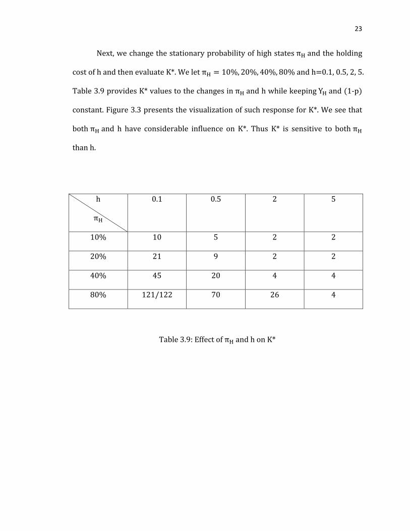
Next, we change the stationary probability of high states πH and the holding
cost of h and then evaluate K*. We let πH = 10%, 20%, 40%, 80% and h=0.1, 0.5, 2, 5.
Table 3.9 provides K* values to the changes in πH and h while keeping YH and (1-p)
constant. Figure 3.3 presents the visualization of such response for K*. We see that
both πH and h have considerable influence on K*. Thus K* is sensitive to both πH
than h.
h
πH
0.1 0.5 2 5
10% 10 5 2 2
20% 21 9 2 2
40% 45 20 4 4
80% 121/122 70 26 4
Table 3.9: Effect of πH and h on K*
24
Figure 3.3: Visualization of the dependence of K* on πH and h
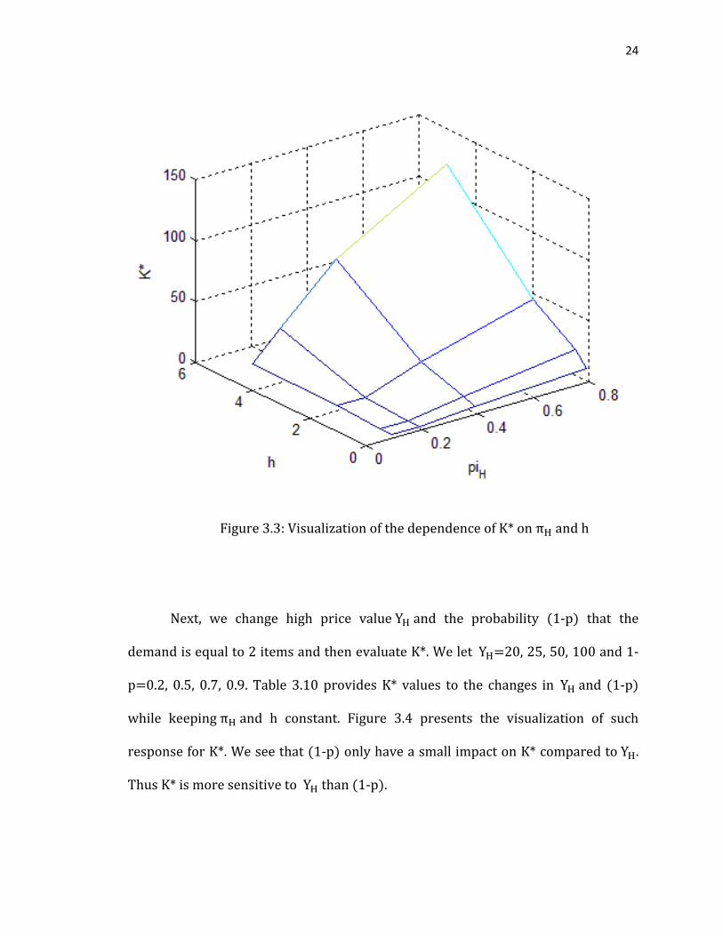
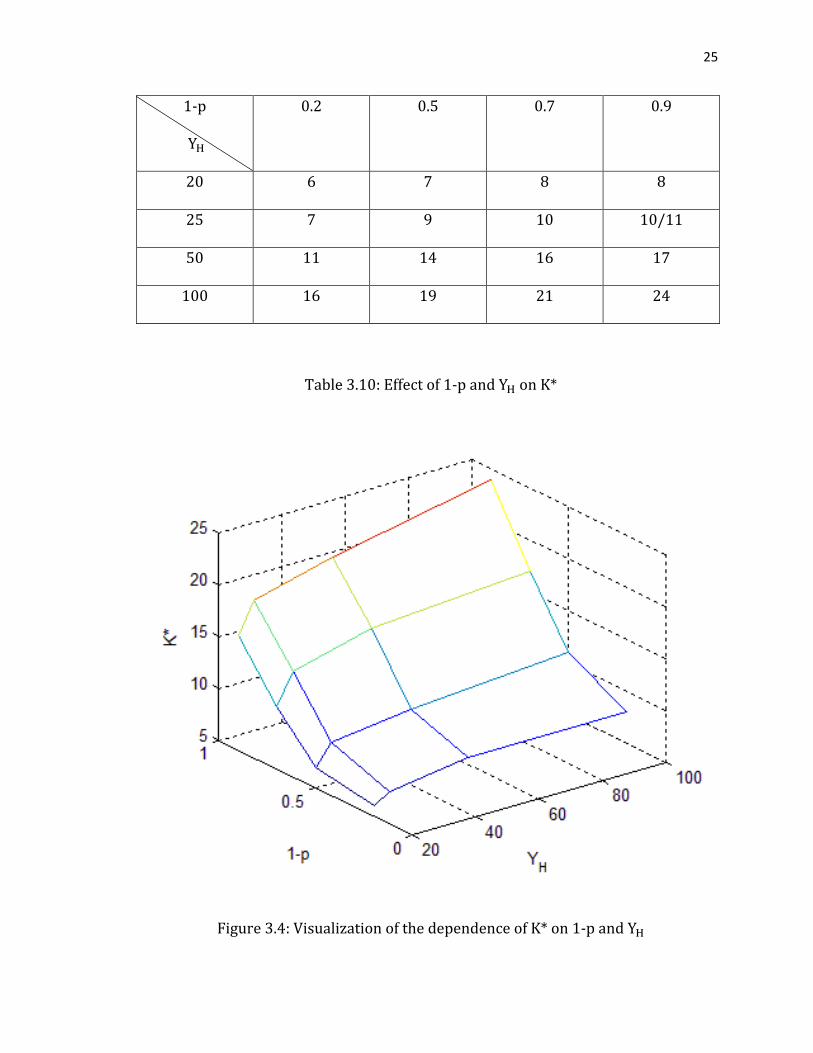
Next, we change high price value YH and the probability (1-p) that the
demand is equal to 2 items and then evaluate K*. We let YH=20, 25, 50, 100 and 1-
p=0.2, 0.5, 0.7, 0.9. Table 3.10 provides K* values to the changes in YH and (1-p)
while keeping πH and h constant. Figure 3.4 presents the visualization of such
response for K*. We see that (1-p) only have a small impact on K* compared to YH.
Thus K* is more sensitive to YH than (1-p).
25
1-p
YH
0.2 0.5 0.7 0.9
20 6 7 8 8
25 7 9 10 10/11
50 11 14 16 17
100 16 19 21 24
Table 3.10: Effect of 1-p and YH on K*
Figure 3.4: Visualization of the dependence of K* on 1-p and YH
26
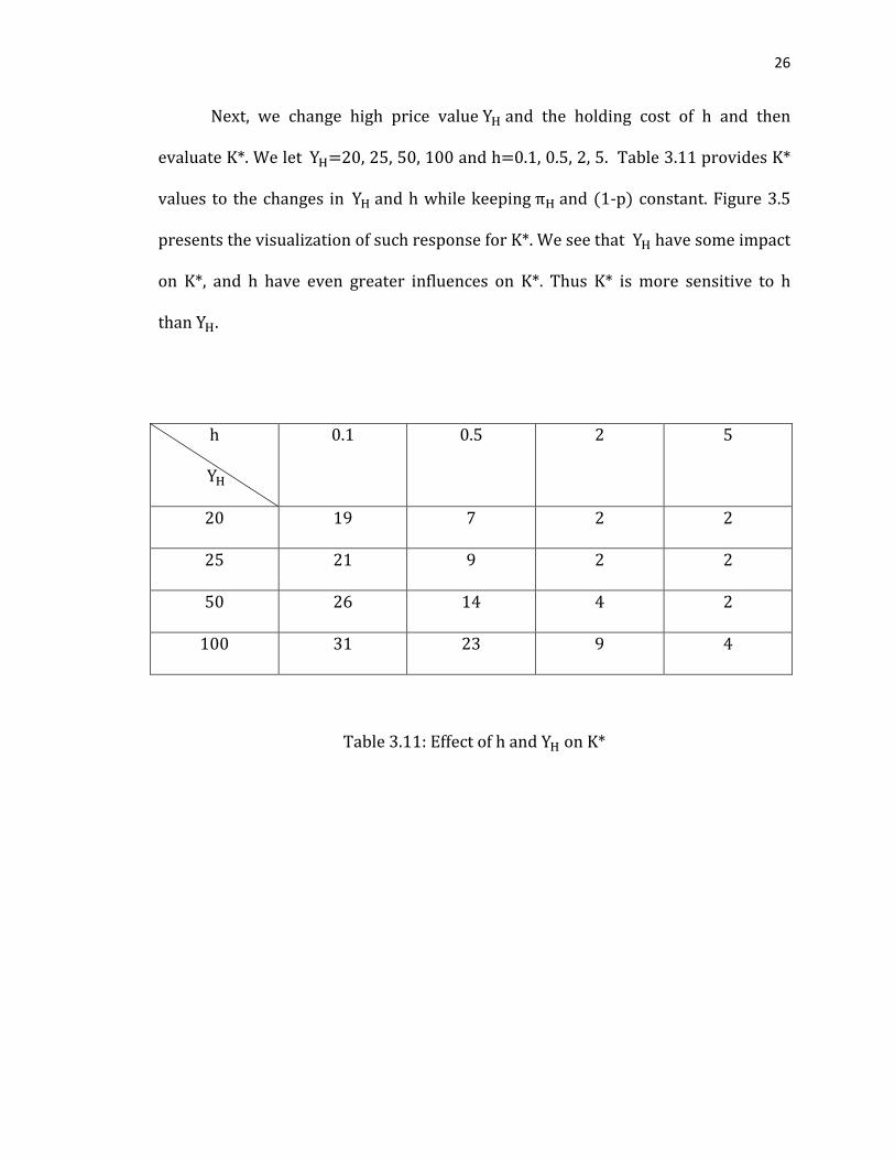
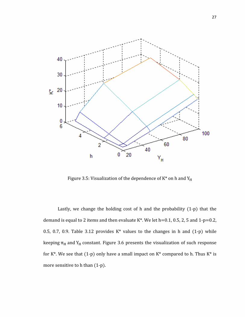
Next, we change high price value YH and the holding cost of h and then
evaluate K*. We let YH=20, 25, 50, 100 and h=0.1, 0.5, 2, 5. Table 3.11 provides K*
values to the changes in YH and h while keeping πH and (1-p) constant. Figure 3.5
presents the visualization of such response for K*. We see that YH have some impact
on K*, and h have even greater influences on K*. Thus K* is more sensitive to h
than YH.
h
YH
0.1 0.5 2 5
20 19 7 2 2
25 21 9 2 2
50 26 14 4 2
100 31 23 9 4
Table 3.11: Effect of h and YH on K*
27
Figure 3.5: Visualization of the dependence of K* on h and YH
Lastly, we change the holding cost of h and the probability (1-p) that the
demand is equal to 2 items and then evaluate K*. We let h=0.1, 0.5, 2, 5 and 1-p=0.2,
0.5, 0.7, 0.9. Table 3.12 provides K* values to the changes in h and (1-p) while
keeping πH and YH constant. Figure 3.6 presents the visualization of such response
for K*. We see that (1-p) only have a small impact on K* compared to h. Thus K* is
more sensitive to h than (1-p).
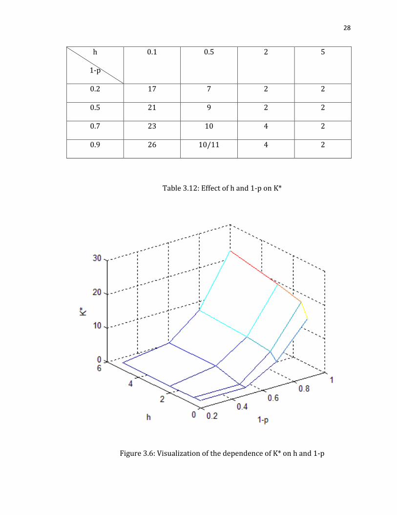
28
h
1-p
0.1 0.5 2 5
0.2 17 7 2 2
0.5 21 9 2 2
0.7 23 10 4 2
0.9 26 10/11 4 2
Table 3.12: Effect of h and 1-p on K*
Figure 3.6: Visualization of the dependence of K* on h and 1-p
29
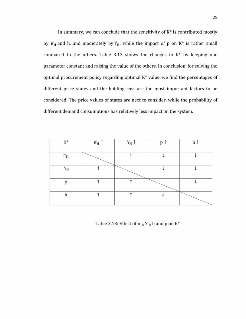
In summary, we can conclude that the sensitivity of K* is contributed mostly
by πH and h, and moderately by YH, while the impact of p on K* is rather small
compared to the others. Table 3.13 shows the changes in K* by keeping one
parameter constant and raising the value of the others. In conclusion, for solving the
optimal procurement policy regarding optimal K* value, we find the percentages of
different price states and the holding cost are the most important factors to be
considered. The price values of states are next to consider, while the probability of
different demand consumptions has relatively less impact on the system.
K* πH ↑ YH ↑ p ↑ h ↑
πH ↑ ↓ ↓
YH ↑ ↓ ↓
p ↑ ↑ ↓
h ↑ ↑ ↓
Table 3.13: Effect of πH, YH, h and p on K*
30
Chapter 4
A Case Study
4.1 Introduction
We consider a company, producing an intermediate material that is
used in manufacturing military as well as consumer products. An expensive rare
metal is required in the production as the raw material. Since the intermediate
material is used in manufacturing military products, we do not allow any back
ordering or lost sales. The procurement problem of rare metal, Y, is to minimize the
total cost of the company including inventory holding, spot buying and contract
buying costs during a finite time horizon.
We have made our case study based on the following assumptions: The
procurement frequency is monthly. Spot buying is a purchase made in the current
month and contract buying is a purchase made at the beginning of every year that
lasts 12 months. That means if we make a long term contract at the beginning of the
year, we pay the total cost at the beginning and receive a delivery every month
throughout the year. Let C(m) denote the spot price at month m, C’(m) denote the
contract price at month m, Q(m) denote the total contract amount for the year of
month m and S(m) denote the amount of spot buying at month m. Assume that the
contract price has a discount of d dollars per kg on the spot price. All purchases are
made at the beginning of the month while demands, D(m), come after the purchases
31
are in the beginning of the month as well. At the end of the month we count the new
inventory level I, also notice all costs at the present have an interest rate of r% as
discount factor and the holding cost are h dollars per kg. It is required that we keep
the inventory level at least twice as large as the last month’s demand. Also, we
assume the inventory level starts with initially 1000kg of rare metal Y, and there is a
capacity limit for spot buying so that the maximum amount that could be bought
every month is 3000kg.
We use a monthly updated linear/dynamic programming model to optimize
this procurement problem. However, some of the data we need are the predicated
values that are coming from a time series autoregressive integrated moving average
(ARIMA) model. The ARIMA model can be used to predict a series of future values
when previous values over a certain time period is available. It fits the distribution
of past data and builds a model to predict future values. More details of the times
series model and ARIMA model can be found in Brockwell & Davis (2002). We use
ARIMA to predict the demand and spot price for a 24month time period in 2010-
2011. We utilize the actual data for those 2 years to validate our forecasting model.
Lastly, we present the optimum procurement policy and compare it to the actual
procurement policy of company X.
32
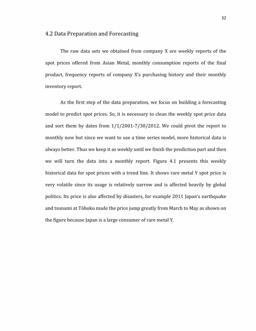
4.2 Data Preparation and Forecasting
The raw data sets we obtained from company X are weekly reports of the
spot prices offered from Asian Metal, monthly consumption reports of the final
product, frequency reports of company X’s purchasing history and their monthly
inventory report.
As the first step of the data preparation, we focus on building a forecasting
model to predict spot prices. So, it is necessary to clean the weekly spot price data
and sort them by dates from 1/1/2001-7/30/2012. We could pivot the report to
monthly now but since we want to use a time series model, more historical data is
always better. Thus we keep it as weekly until we finish the prediction part and then
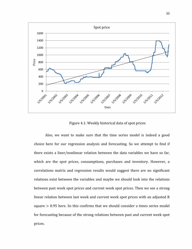
we will turn the data into a monthly report. Figure 4.1 presents this weekly
historical data for spot prices with a trend line. It shows rare metal Y spot price is
very volatile since its usage is relatively narrow and is affected heavily by global
politics. Its price is also affected by disasters, for example 2011 Japan’s earthquake
and tsunami at Tōhoku made the price jump greatly from March to May as shown on
the figure because Japan is a large consumer of rare metal Y.
33
Figure 4.1: Weekly historical data of spot prices
Also, we want to make sure that the time series model is indeed a good
choice here for our regression analysis and forecasting. So we attempt to find if
there exists a liner/nonlinear relation between the data variables we have so far,
which are the spot prices, consumptions, purchases and inventory. However, a
correlations matrix and regression results would suggest there are no significant
relations exist between the variables and maybe we should look into the relations
between past week spot prices and current week spot prices. Then we see a strong
linear relation between last week and current week spot prices with an adjusted R
square > 0.95 here. So this confirms that we should consider a times series model
for forecasting because of the strong relations between past and current week spot
prices.
0
200
400
600
800
1000
1200
1400
1600Pr
ice
Date
Spot price
34
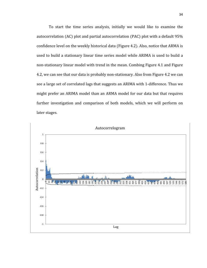
To start the time series analysis, initially we would like to examine the
autocorrelation (AC) plot and partial autocorrelation (PAC) plot with a default 95%
confidence level on the weekly historical data (Figure 4.2). Also, notice that ARMA is
used to build a stationary linear time series model while ARIMA is used to build a
non-stationary linear model with trend in the mean. Combing Figure 4.1 and Figure
4.2, we can see that our data is probably non-stationary. Also from Figure 4.2 we can
see a large set of correlated lags that suggests an ARIMA with 1-difference. Thus we
might prefer an ARIMA model than an ARMA model for our data but that requires
further investigation and comparison of both models, which we will perform on
later stages.
-1
-0.8
-0.6
-0.4
-0.2
0
0.2
0.4
0.6
0.8
1
0 13 26 39 52 65 78 91 104
117
130
143
156
169
182
195
208
221
234
247
260
273
286
299
312
325
338
351
364
377
390
403
416
429
442
455
468
481
494
507
520
533
546
559
572
585
Auto
corr
elat
ion
Lag
Autocorrelogram
35
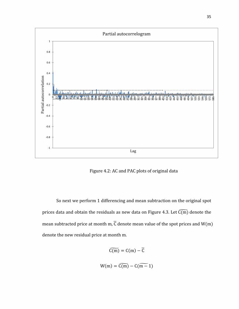
Figure 4.2: AC and PAC plots of original data
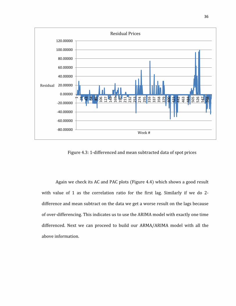
So next we perform 1 differencing and mean subtraction on the original spot
prices data and obtain the residuals as new data on Figure 4.3. Let C(m)� denote the
mean subtracted price at month m, C denote mean value of the spot prices and W(m)
denote the new residual price at month m.
C(m)� = C(m) − C
W(m) = C(m)� − C(m − 1)�
-1
-0.8
-0.6
-0.4
-0.2
0
0.2
0.4
0.6
0.8
1
0 13 26 39 52 65 78 91 104
117
130
143
156
169
182
195
208
221
234
247
260
273
286
299
312
325
338
351
364
377
390
403
416
429
442
455
468
481
494
507
520
533
546
559
572
585
Part
ial a
utoc
orre
latio
n
Lag
Partial autocorrelogram
36
Figure 4.3: 1-differenced and mean subtracted data of spot prices
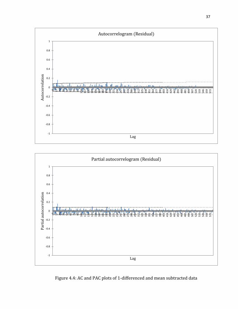
Again we check its AC and PAC plots (Figure 4.4) which shows a good result
with value of 1 as the correlation ratio for the first lag. Similarly if we do 2-
difference and mean subtract on the data we get a worse result on the lags because
of over-differencing. This indicates us to use the ARIMA model with exactly one time
differenced. Next we can proceed to build our ARMA/ARIMA model with all the
above information.
-80.00000
-60.00000
-40.00000
-20.00000
0.00000
20.00000
40.00000
60.00000
80.00000
100.00000
120.00000
1 22 43 64 85 106
127
148
169
190
211
232
253
274
295
316
337
358
379
400
421
442
463
484
505
526
547
568
Residual
Week #
Residual Prices
37
Figure 4.4: AC and PAC plots of 1-differenced and mean subtracted data
-1
-0.8
-0.6
-0.4
-0.2
0
0.2
0.4
0.6
0.8
1
0 13 26 39 52 65 78 91 104
117
130
143
156
169
182
195
208
221
234
247
260
273
286
299
312
325
338
351
364
377
390
403
416
429
442
455
468
481
494
507
520
533
546
559
572
Auto
corr
elat
ion
Lag
Autocorrelogram (Residual)
-1
-0.8
-0.6
-0.4
-0.2
0
0.2
0.4
0.6
0.8
1
0 13 26 39 52 65 78 91 104
117
130
143
156
169
182
195
208
221
234
247
260
273
286
299
312
325
338
351
364
377
390
403
416
429
442
455
468
481
494
507
520
533
546
559
572
Part
ial a
utoc
orre
latio
n
Lag
Partial autocorrelogram (Residual)
38
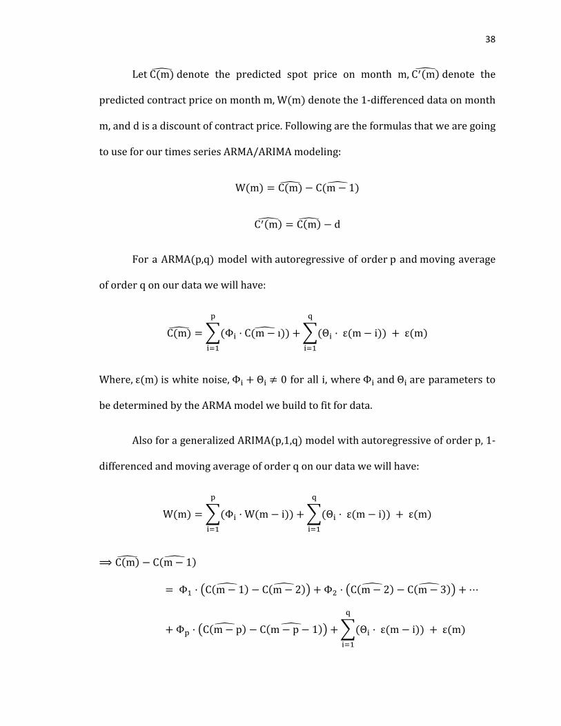
Let C(m)� denote the predicted spot price on month m, C′(m)� denote the
predicted contract price on month m, W(m) denote the 1-differenced data on month
m, and d is a discount of contract price. Following are the formulas that we are going
to use for our times series ARMA/ARIMA modeling:
W(m) = C(m)� − C(m − 1)�
C′(m)� = C(m)� − d
For a ARMA(p,q) model with autoregressive of order p and moving average
of order q on our data we will have:
C(m)� = �(Φi
p
i=1
· C(m − ı)� ) + �(Θi
q
i=1
· ε(m − i)) + ε(m)
Where, ε(m) is white noise, Φi + Θi ≠ 0 for all i, where Φi and Θi are parameters to
be determined by the ARMA model we build to fit for data.
Also for a generalized ARIMA(p,1,q) model with autoregressive of order p, 1-
differenced and moving average of order q on our data we will have:
W(m) = �(Φi
p
i=1
· W(m − i)) + �(Θi
q
i=1
· ε(m − i)) + ε(m)
⟹ C(m)� − C(m − 1)�
= Φ1 · �C(m − 1)� − C(m − 2)� � + Φ2 · �C(m − 2)� − C(m − 3)� � + ⋯
+ Φp · �C(m − p)� − C(m − p − 1)� � + �(Θi
q
i=1
· ε(m − i)) + ε(m)
39
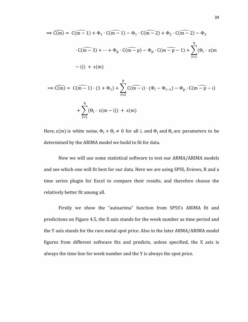
⟹ C(m)� = C(m − 1)� + Φ1 · C(m − 1)� − Φ1 · C(m − 2)� + Φ2 · C(m − 2)� − Φ2
· C(m − 3)� + ⋯ + Φp · C(m − p)� − Φp · C(m − p − 1)� + �(Θi
q
i=1
· ε(m
− i)) + ε(m)
⟹ C(m)� = C(m − 1)� · (1 + Φ1) + � C(m − ı)� · (Φi
p
i=2
− Φi−1) − Φp · C(m − p − ı)�
+ �(Θi
q
i=1
· ε(m − i)) + ε(m)
Here, ε(m) is white noise, Φi + Θi ≠ 0 for all i, and Φi and Θi are parameters to be
determined by the ARIMA model we build to fit for data.
Now we will use some statistical software to test our ARMA/ARIMA models
and see which one will fit best for our data. Here we are using SPSS, Eviews, R and a
time series plugin for Excel to compare their results, and therefore choose the
relatively better fit among all.
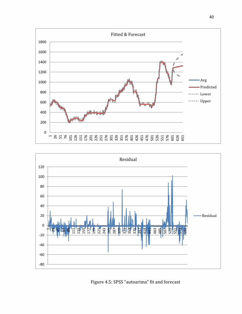
Firstly we show the “autoarima” function from SPSS’s ARIMA fit and
predictions on Figure 4.5, the X axis stands for the week number as time period and
the Y axis stands for the rare metal spot price. Also in the later ARMA/ARIMA model
figures from different software fits and predicts, unless specified, the X axis is
always the time line for week number and the Y is always the spot price.
40
Figure 4.5: SPSS “autoarima” fit and forecast
0
200
400
600
800
1000
1200
1400
1600
1800
1 26 51 76 101
126
151
176
201
226
251
276
301
326
351
376
401
426
451
476
501
526
551
576
601
626
651
Fitted & Forecast
Avg
Predicted
Lower
Upper
-80
-60
-40
-20
0
20
40
60
80
100
120
1 23 45 67 89 111
133
155
177
199
221
243
265
287
309
331
353
375
397
419
441
463
485
507
529
551
573
595
Residual
Residual
41
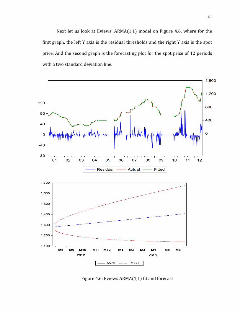
Next let us look at Eviews’ ARMA(1,1) model on Figure 4.6, where for the
first graph, the left Y axis is the residual thresholds and the right Y axis is the spot
price. And the second graph is the forecasting plot for the spot price of 12 periods
with a two standard deviation line.
Figure 4.6: Eviews ARMA(1,1) fit and forecast
42
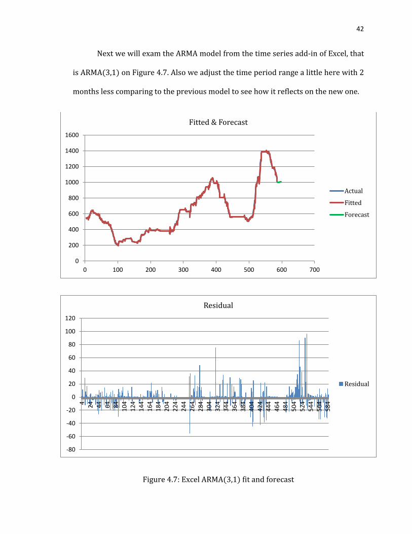
Next we will exam the ARMA model from the time series add-in of Excel, that
is ARMA(3,1) on Figure 4.7. Also we adjust the time period range a little here with 2
months less comparing to the previous model to see how it reflects on the new one.
Figure 4.7: Excel ARMA(3,1) fit and forecast
0
200
400
600
800
1000
1200
1400
1600
0 100 200 300 400 500 600 700
Fitted & Forecast
Actual
Fitted
Forecast
-80
-60
-40
-20
0
20
40
60
80
100
120
4 24 44 64 84 104
124
144
164
184
204
224
244
264
284
304
324
344
364
384
404
424
444
464
484
504
524
544
564
584
Residual
Residual
43
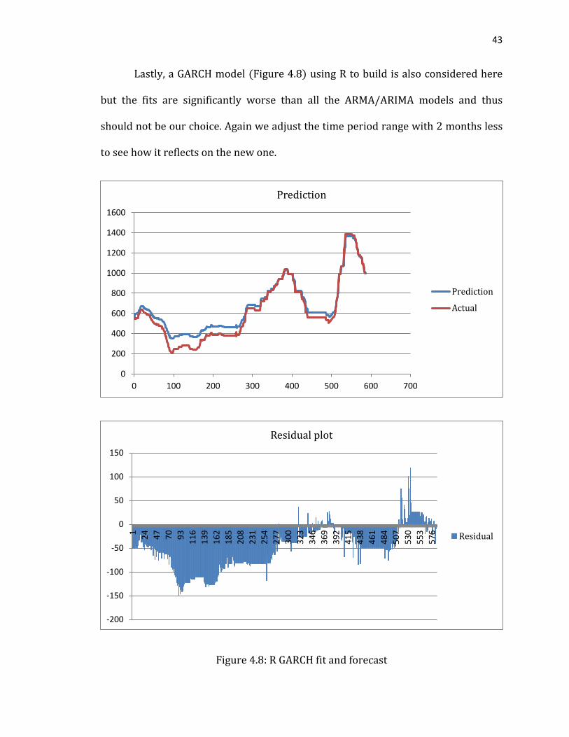
Lastly, a GARCH model (Figure 4.8) using R to build is also considered here
but the fits are significantly worse than all the ARMA/ARIMA models and thus
should not be our choice. Again we adjust the time period range with 2 months less
to see how it reflects on the new one.
Figure 4.8: R GARCH fit and forecast
0
200
400
600
800
1000
1200
1400
1600
0 100 200 300 400 500 600 700
Prediction
Prediction
Actual
-200
-150
-100
-50
0
50
100
150
1 24 47 70 93 116
139
162
185
208
231
254
277
300
323
346
369
392
415
438
461
484
507
530
553
576
Residual plot
Residual

44
In summary, the time series model we choose to use for our forecasting
should not only be a best fit of past data, but also a most accurate and correct model
for forecasting data. Notice that from all of the above models we see a huge misfit
around week 500-540. That is around year 2011 when Tōhoku earthquake and
tsunami happened in Japan and its aftermath affected the market price of rare metal
Y. We understand that such an unpredictable event happened all the time but it
should not affect our model in a general sense. Now considering the fitting part, we
conclude that ARMA(3,1) from Excel and “autoarima” from SPSS have a better
performance. In order to see which forecast data performs better, since year 2010-
2011 are the most unpredictable two years, we take the historical data from 2001-
2009 and let all models to forecast 2010-2011 data to compare them with the actual
data we have. Therefore although both ARMA(3,1) and “autoarima” were providing
models with good fit for past data, “autoarima” from SPSS showed us a better
forecasting ability. Thus we choose “autoarima” function from SPSS to do our
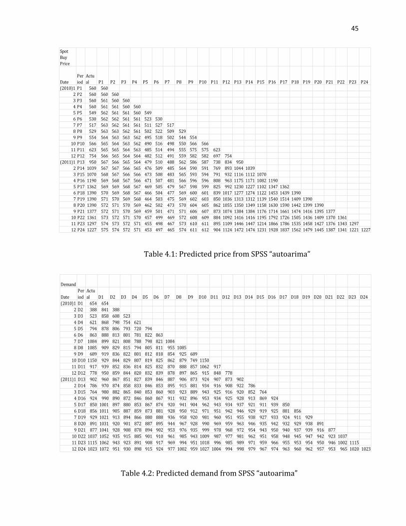
forecasting with the results below on Table 4.1. As you can see, in a long turn, the
price forecasting could make a large error comparing to the actual values. However,
in our dynamic model for optimization we would only require for the next time
period predicted value which usually is accurate enough and acceptable.
We can also do similar analysis on the demand forecasting part which
contains a much smaller historical data set. Since we assume the company is always
going to fulfill the demand, demand values are not as sensitive as the price. Thus we
omit the procedures of the demand forecasting and provide the result directly on
Table 4.2 below.
45
Table 4.1: Predicted price from SPSS “autoarima”
Table 4.2: Predicted demand from SPSS “autoarima”
Spot Buy Price
DatePeriod
Actual P1 P2 P3 P4 P5 P6 P7 P8 P9 P10 P11 P12 P13 P14 P15 P16 P17 P18 P19 P20 P21 P22 P23 P24
(2010)1 P1 560 5602 P2 560 560 5603 P3 560 561 560 5604 P4 560 561 561 560 5605 P5 549 562 561 561 560 5496 P6 530 562 562 561 561 523 5307 P7 517 563 562 561 561 511 527 5178 P8 529 563 563 562 561 502 522 509 5299 P9 554 564 563 563 562 495 518 502 544 554
10 P10 566 565 564 563 562 490 516 498 550 566 56611 P11 623 565 565 564 563 485 514 494 555 575 575 62312 P12 754 566 565 564 564 482 512 491 559 582 582 697 754
(2011)1 P13 950 567 566 565 564 479 510 488 562 586 587 738 834 9502 P14 1039 567 567 566 565 476 509 485 564 590 591 769 893 1044 10393 P15 1070 568 567 566 566 473 508 483 565 593 594 791 932 1116 1112 10704 P16 1190 569 568 567 566 471 507 481 566 596 596 808 963 1175 1171 1082 11905 P17 1362 569 569 568 567 469 505 479 567 598 599 825 992 1230 1227 1102 1347 13626 P18 1390 570 569 568 567 466 504 477 569 600 601 839 1017 1277 1274 1122 1453 1439 13907 P19 1390 571 570 569 568 464 503 475 569 602 603 850 1036 1313 1312 1139 1540 1514 1409 13908 P20 1390 572 571 570 569 462 502 473 570 604 605 862 1055 1350 1349 1158 1630 1590 1442 1399 13909 P21 1377 572 571 570 569 459 501 471 571 606 607 873 1074 1384 1384 1176 1714 1661 1474 1416 1395 1377
10 P22 1361 573 572 571 570 457 499 469 572 608 609 884 1092 1416 1416 1195 1792 1726 1505 1436 1409 1370 136111 P23 1297 574 573 572 571 455 498 467 573 610 611 895 1109 1446 1447 1214 1866 1786 1535 1458 1427 1376 1343 129712 P24 1227 575 574 572 571 453 497 465 574 611 612 904 1124 1472 1474 1231 1928 1837 1562 1479 1445 1387 1341 1221 1227
Demand
DatePeriod
Actual D1 D2 D3 D4 D5 D6 D7 D8 D9 D10 D11 D12 D13 D14 D15 D16 D17 D18 D19 D20 D21 D22 D23 D24
(2010)1 D1 654 6542 D2 388 841 3883 D3 523 858 608 5234 D4 621 868 798 754 6215 D5 794 878 806 793 720 7946 D6 863 888 813 801 781 822 8637 D7 1084 899 821 808 788 798 821 10848 D8 1085 909 829 815 794 805 811 955 10859 D9 689 919 836 822 801 812 818 854 925 689
10 D10 1150 929 844 829 807 819 825 862 879 749 115011 D11 917 939 852 836 814 825 832 870 888 857 1062 91712 D12 778 950 859 844 820 832 839 878 897 865 915 848 778
(2011)1 D13 902 960 867 851 827 839 846 887 906 873 924 907 873 9022 D14 786 970 874 858 833 846 853 895 915 881 934 916 908 922 7863 D15 764 980 882 865 840 853 860 903 923 889 943 925 916 920 852 7644 D16 924 990 890 872 846 860 867 911 932 896 953 934 925 928 913 869 9245 D17 850 1001 897 880 853 867 874 920 941 904 962 943 934 937 921 911 939 8506 D18 856 1011 905 887 859 873 881 928 950 912 971 951 942 946 929 919 925 881 8567 D19 929 1021 913 894 866 880 888 936 958 920 981 960 951 955 938 927 933 924 911 9298 D20 891 1031 920 901 872 887 895 944 967 928 990 969 959 963 946 935 942 932 929 938 8919 D21 877 1041 928 908 878 894 902 953 976 935 999 978 968 972 954 943 950 940 937 939 916 877
10 D22 1037 1052 935 915 885 901 910 961 985 943 1009 987 977 981 962 951 958 948 945 947 942 923 103711 D23 1115 1062 943 923 891 908 917 969 994 951 1018 996 985 989 971 959 966 955 953 954 950 946 1002 111512 D24 1023 1072 951 930 898 915 924 977 1002 959 1027 1004 994 998 979 967 974 963 960 962 957 953 965 1020 1023
46
4.3 Modeling
After we did our data preparation including the data forecasting, we had all
the data we need for the model. Now we have all the data including actual demand,
predicted demand, actual spot price, predicted spot price, actual contract price,
predicted contract price, actual procurement purchases and actual inventory levels.
Notice for the spot price and demand in our dynamic programming, they will not all
be the actual values but as a hybrid of both actual values and predicted values. And
with the updates move on, our dynamic system will substitute the old predicted
values with the recently obtained actual values and require new predicted values
from ARMA/ARIMA forecasting model.
Next, we shall start to build our linear programming model to minimize the
expected total cost of each month.
Total cost of month m:
T(m) = �
C(m) · S(m) + C′(m) · Q(m) + h · I(m),for m is a beginning month of the year
C(m) · S(m) + h · I(m), for m otherwise
C′(m) and Q(m) are determined by the beginning of the year since it is a long term
contract price and will be decide at the beginning of month 1, 13, 25…etc.
The following constraints will ensure the validity of the assumptions.
47
Inventory level of month m:
I(m) = I(m − 1) + S(m) + Q(m) − D(m)
I(m) ≥ 12 D(m − 1)
Procurement policy of month m:
0 ≤ S(m) ≤ 2
Q(m) > 0
Contract buy and spot buy relations at month m:
C′(m) = C(m) − d
With this linear program of every month m, we can then extend it to a multi
period mathematical programming model with the objective of minimizing the total
cost of all time periods in a finite horizon. Let M be the total number of months. Thus,
we have the mathematical programming model as the following.
Minimize the total cost of all M months considering interest rate r:
T(M) = � �1
1 + r�m
[C(m) · S(m) · +h · I(m)]M
m=1
+ � �1
1 + r�f
C′(f) · Q(f)f=1,13,25…
Such that:
I(m) = I(m − 1) + S(m) + Q(m) − D(m)
I(m) ≥12
D(m − 1)
48
C′(m) = C(m) − d
0 ≤ S(m) ≤ 2, Q(m) > 0
Notice that all the values can be imported from our data preparation stage, and then
plugged into the above system starting for m=1…M.
This means we have to run the linear programming repeatedly while
updating the predicted data and plug in new actual data to solve the problem M
times until the end. We approach to do so by using Xpress Mosel while
incorporating it with updated ARIMA models imported from SPSS. Now let us try
our algorithm based on all the assumptions we have made before and test its
efficiency for the year of 2010-2011, since they are the most unpredictable years,
and would sort of serve us as the worst case scenario. In this case M=24 and
January of 2010 will be m=1.
The codes we use to build the above single time period model in Xpress
Mosel can be found in Appendix B, where the spot price C and demand D are in a
hybrid fashion containing both actual values from historical data and predicted
values from ARIMA model.
4.4 Optimization Result
Eventually, we want to compare our optimum procurement policy with the
actual procurement company X made during 2010-2011 and by inserting different
49
interest rate or holding cost we can also simulate the policy under different
scenarios. Here we would like to show one of the most basic scenarios with h = 10,
d = 50 and r = 0.0006. Also, since it is a simulation for year 2010-2011, M = 1…24
and F = 1…2. Since we are doing this linear programming optimization with updates,
only every month’s spot buying strategy will be adopted and the inventory will rely
on the actually demand in the future rather than the predicted values from ARIMA
model. That is, using the new spot price we observe, demand predictions from the
ARIMA model and the policy we have adopted last month via the linear
programming model, we run the linear program to compute a new inventory level,
thus decide on the order quantity. The linear programming model is applied
repeatedly in order to provide the next month’s procurement policy as well as
calculate the new inventory level. Eventually, we will reach our last time period and
then we can consolidate the entire spot buy, contract buy and inventory level
control record for all months.
In summary, by running the above Xpress Mosel model over 24 months with
each time importing a new updated data from ARMA/ARIMA, we have the result for
every month’s spot buying and contract buying amount, as well as the inventory
levels. Finally, the optimum expected total cost is: $15,922,901, with a total
purchase of 21937 kg of rare metal Y and average of $726/kg, the detailed optimal
policy is at the following.
Spot buying quantity of month 1-24: all zeros kg.
Contract buying quantity of year 2010 and 2011: 11167kg and 10770kg.
50
Inventory level of the month 1-24: 1276kg, 1819kg, 2227kg, 2536kg, 2673kg,
2740kg, 2587kg, 2432kg, 2674kg, 2455kg, 2468kg, 2621kg, 2616kg, 2728kg, 2861kg,
2835kg, 2882kg, 2924kg, 2892kg, 2899kg, 2919kg, 2780kg, 2562kg, 2437kg.
When we compare the optimum procurement policy to company X’s actual
purchases, we see that they have made a total purchase of 19983kg of rare metal Y
and total cost of $17,165,381 with average purchase of $ 859/kg, we have spent 7.8%
less on the total cost and 18.3% less per kg on rare metal of Y while doing more
purchasing. Thus, it strongly suggests that our approach would provide
considerable savings for the total cost.
51
Chapter 5
Conclusions
In this thesis, we study various methods for optimal procurement policy
under different circumstances of our own. Firstly, in chapter 3, we use a policy that
its form is given as a base-stock policy and try to find the best base-stock value K*.
Also, we investigate the impact of various parameters on the optimal base-stock
value. Secondly, in chapter 4, we approach a real life scenario where we have to
provide an optimal procurement policy from historical data. We applied time series
modeling to provide raw material price and demand forecasts that will be used in a
mathematical program. This mathematical program is solved recursively by
updating the price and demand forecasts at each time step. In this case study, we
show that inventory/procurement costs can be reduced by implementing our
algorithm. In future, we plan to investigate properties and structure of the optimum
policy for procurement and production planning. We are especially interested in
threshold type policies that are easy to implement.
52
Appendix A
The coding for the expected total cost respect to different values of K in
Matlab when K ≥ 5 is below.
%K >= 5
function total = totalcost(K)
% Parameters
a = 20/108;
b = 5/108;
p = 0.5;
k = K-1;
h = 0.5;
YL = 15;
YH = 25;
% Build the matrix
A = [ones(1,k); zeros(1,k); zeros(k-2,1) (diag(-ones(1,k-2))+diag((1-
a)*p*ones(1,k-3),1)+diag((1-a)*(1-p)*ones(1,k-4),2)) zeros(k-2,1)];
A(2,1) = -a;
A(2,2) = 1-a;
53
A(2,3) = (1-a)*(1-p);
A(k-1,k) = b*(1-p);
A(k,k) = b*p;
B = zeros(k,1);
B(1) = 1;
% Solve all the pi
mypiT = A\B;
mypi = (mypiT)';
display(mypi);
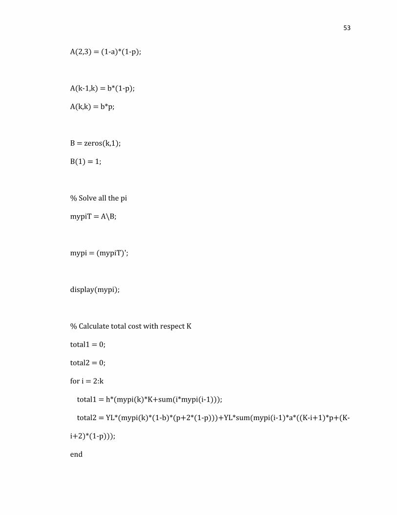
% Calculate total cost with respect K
total1 = 0;
total2 = 0;
for i = 2:k
total1 = h*(mypi(k)*K+sum(i*mypi(i-1)));
total2 = YL*(mypi(k)*(1-b)*(p+2*(1-p)))+YL*sum(mypi(i-1)*a*((K-i+1)*p+(K-
i+2)*(1-p)));
end

54
total3 = YH*(mypi(1)*(1-a)*(p+2*(1-p))+mypi(2)*(1-a)*(1-p));
total = total1 + total2 + total3;
display(K);
55
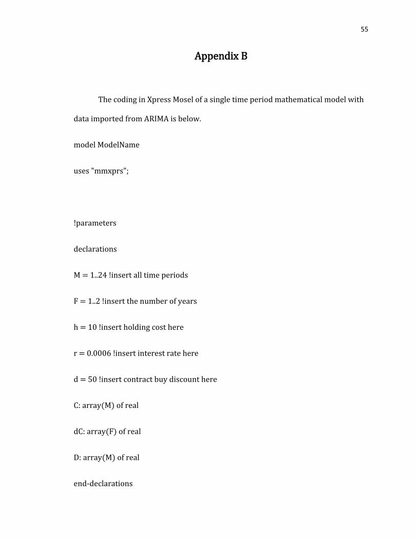
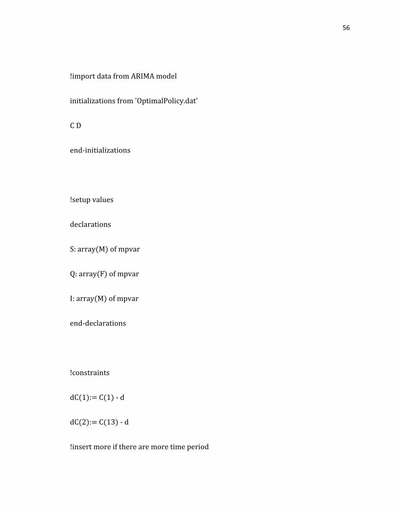
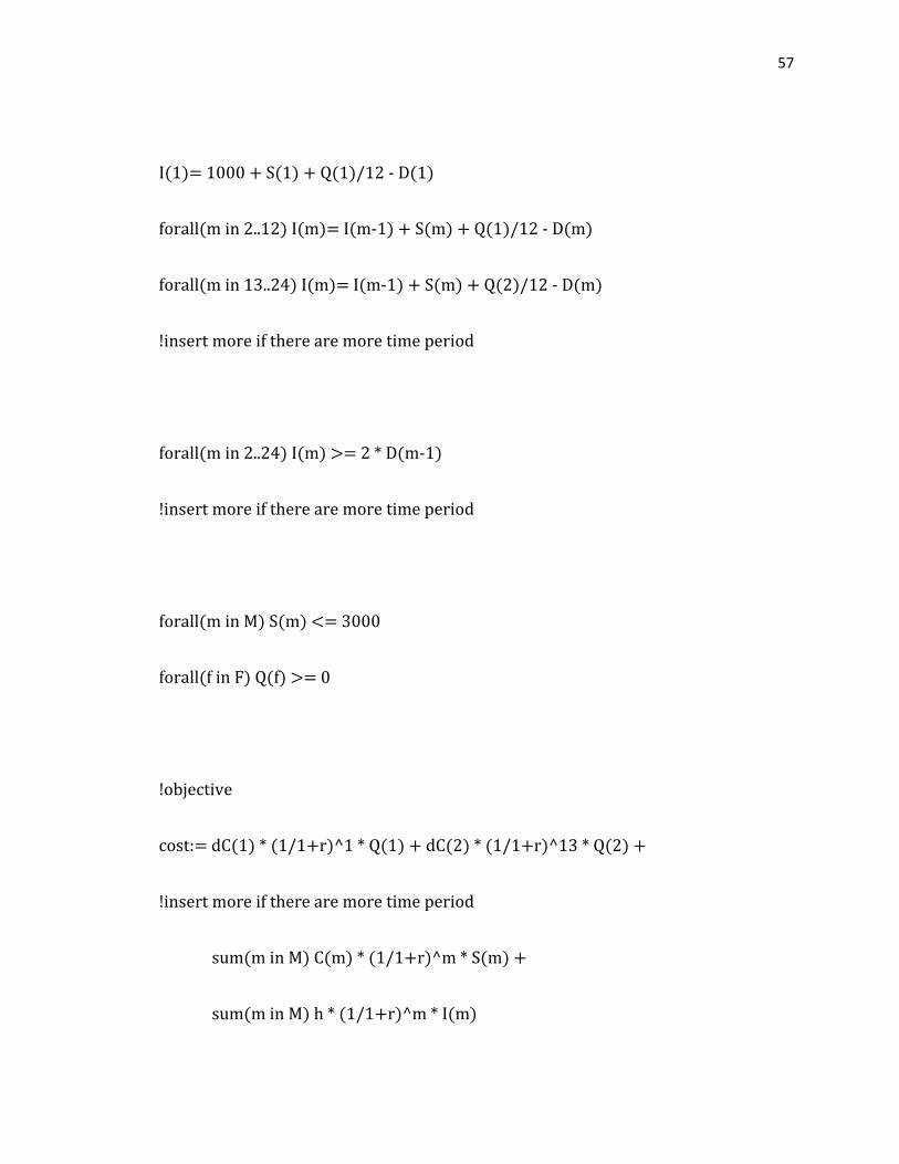
Appendix B
The coding in Xpress Mosel of a single time period mathematical model with
data imported from ARIMA is below.
model ModelName
uses "mmxprs";
!parameters
declarations
M = 1..24 !insert all time periods
F = 1..2 !insert the number of years
h = 10 !insert holding cost here
r = 0.0006 !insert interest rate here
d = 50 !insert contract buy discount here
C: array(M) of real
dC: array(F) of real
D: array(M) of real
end-declarations
56
!import data from ARIMA model
initializations from 'OptimalPolicy.dat'
C D
end-initializations
!setup values
declarations
S: array(M) of mpvar
Q: array(F) of mpvar
I: array(M) of mpvar
end-declarations
!constraints
dC(1):= C(1) - d
dC(2):= C(13) - d
!insert more if there are more time period
57
I(1)= 1000 + S(1) + Q(1)/12 - D(1)
forall(m in 2..12) I(m)= I(m-1) + S(m) + Q(1)/12 - D(m)
forall(m in 13..24) I(m)= I(m-1) + S(m) + Q(2)/12 - D(m)
!insert more if there are more time period
forall(m in 2..24) I(m) >= 2 * D(m-1)
!insert more if there are more time period
forall(m in M) S(m) <= 3000
forall(f in F) Q(f) >= 0
!objective
cost:= dC(1) * (1/1+r)^1 * Q(1) + dC(2) * (1/1+r)^13 * Q(2) +
!insert more if there are more time period
sum(m in M) C(m) * (1/1+r)^m * S(m) +
sum(m in M) h * (1/1+r)^m * I(m)

58
!solve
minimize(cost)
writeln("Begin running model")
writeln("The minimum of the total cost is: ", getobjval)
forall(m in M) writeln("Spot buy quantity of month(", m, "): ", getsol(S(m)))
forall(f in F) writeln("Contract buy quantity of year(", f, "): ", getsol(Q(f)))
forall(m in M) writeln("Inventory level of the month(", m, "): ", getsol(I(m)))
writeln("End running model")
end-model
59
References
Brockwell, P. J., & Davis, R. A. (2002). Introduction to Time Series and Forecasting (2nd ed.). New York: Springer.
Goel, A., & Gutierrez, G. J. (2012). Integrating Commodity Markets in the Optimal Procurement Policies of a Stochastic Inventory System. Social Science Research Network, from http://dx.doi.org/10.2139/ssrn.930486.
Hwang, H., & Hahn, K. (2000). An optimal procurement policy for items with an inventory level-dependent demand rate and fixed lifetime. European Journal of Operational Research, 127(3), 537-545.
Inderfurth, K., Kelle, P., & Kleber, R. (2013). Dual Sourcing Using Capacity Reservation and Spot Market: Optimal Procurement Policy and Heuristic Parameter Determination. European Journal of Operational Research, 225(2), 298-309.
Nagarajan, M., & Rajagopalan, R. S. (2009). A Multi-Period Model of Inventory Competition. Social Science Research Network, from http://dx.doi.org/10.2139/ssrn.1140311.
Polatoglu, H., & Sahin, I. (2000). Optimal procurement policies under price-dependent demand. International Journal of Production Economics, 65(2), 141-171.
Secomandi, N., & Kekre, S. (2009). Commodity Procurement with Demand Forecast and Forward Price Updates. Tepper School of Business, Paper 221.
Seifert, R. W., Thonemann, U. W., & Hausman, W. H. (2004). Optimal procurement strategies for online spot markets. European Journal of Operational Research, 152(3), 781-799.
Zhang, W., Chen, Y., Hua, Z., & Xue, W. (2011). Optimal Policy with a Total Order Quantity Commitment Contract in the Presence of a Spot Market. Journal of Systems Science and Systems Engineering, 20(1), 25-42.