Embed Size (px)
Citation preview
8/6/2019 Optimal Property Management Strategies_Research
http://slidepdf.com/reader/full/optimal-property-management-strategiesresearch 1/25
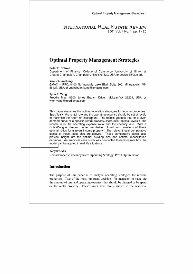
Optimal Property Management Strategies 1
INTERNATIONAL REAL ESTATE REVIEW2001 Vol. 4 No. 1: pp. 1 - 25
Optimal Property Management Strategies
Peter F. ColwellDepartment of Finance, College of Commerce, University of Illinois atUrbana-Champaign, Champaign, Illinois 61820, USA or [email protected]
Yuehchuan KungGMAC – RFC, 8400 Normandale Lake Blvd. Suite 600, Minneapolis, MN55437, USA or [email protected]
Tyler T. YangFreddie Mac, 8200 Jones Branch Drive., McLean,VA 22209, USA [email protected]
This paper examines the optimal operation strategies for income properties.Specifically, the rental rate and the operating expense should be set at levelsto maximize the return on investment. The results suggest that for a givendemand curve of a specific rental property, there exist optimal levels of theincome ratio, the operating expense ratio, and the vacancy rate. With aCobb-Douglas demand curve, we derived closed form solutions of theseoptimal ratios for a given income property. The relevant local comparativestatics of these ratios also are derived. These comparative statics alsoprovide insight into the optimal building size and optimal rehabilitationdecisions. An empirical case study was conducted to demonstrate how the
model can be applied in real life situations.
KeywordsRental Property; Vacancy Rate; Operating Strategy; Profit Optimization
Introduction
The purpose of this paper is to analyze operating strategies for incomeproperties. Two of the most important decisions for managers to make arethe amount of rent and operating expenses that should be charged or be spenton the rental property. These issues were rarely studied in the academic
8/6/2019 Optimal Property Management Strategies_Research
http://slidepdf.com/reader/full/optimal-property-management-strategiesresearch 2/25
2 Colwell, Kung and Yang
literature. In this paper, we attack this problem by assuming that themanager's objective is to maximize the net present value ( NPV ) of theinvestment.
Colwell (1991) indicated that, under a given market condition, a highervacancy rate might actually be preferable to a lower vacancy rate. He used a
downward sloping curve between occupancy rate and gross rental rate toillustrate that, within a relevant range, per-unit rent must fall if occupancy isto rise. A completely occupied building may not provide the maximumpossible net operating income ( NOI ) to the property owner. Colwellconcluded that in maximizing value, achieving a precise balance in incomeand expenses might be more important than reaching 100-percent occupancy.
Chinloy and Maribojoc (1998) used a portfolio of apartment buildings inPortland, Oregon, to test whether managers have flexibility to selectstrategies on expense (overhead, repairs, capital expenditures, taxes andinsurance, and marketing)-rent combinations. They found a positivecorrelation between gross rents and expenses. However, the correlationcoefficients between net rents and expenses are not always positive. NOI
increases with an increase in the marketing expense, but decreases with anincrease in other expenses. They contended that optimization at the margin isnot always achieved. There is scope for increases at the margin in certainexpense categories and reduction in others, though partly mitigated by thelumpiness of investments.
In the next section, we introduce the profit maximization decisions faced byan investor. Algebraic properties of the optimal operating ratios are alsointroduced. In Section 3, we use a Cobb-Douglas demand curve todemonstrate the maximization solution more precisely. Comparative staticsof the closed-form solutions of the optimal strategies are derived in Section 4.From these comparatives, implications regarding the optimal building sizeand optimal rehabilitation strategy are also discussed. An empirical analysis
is conducted and summarized in Section 5. The corresponding optimaloperating ratios and their sensitivities confirm with the algebraic solutions.The last section provides conclusions and possible extensions.
The Optimization Framework
Cannaday and Yang (1995, 1996) discussed real estate investor's optimalfinancial decisions (i.e. the optimal interest rate-discount points combinationand the optimal leverage ratio strategies) of income-producing properties.Both studies focus on income-producing properties, and are based on adiscounted cash flow approach. In this paper, we adopt the identical
8/6/2019 Optimal Property Management Strategies_Research
http://slidepdf.com/reader/full/optimal-property-management-strategiesresearch 3/25
Optimal Property Management Strategies 3
approach. Instead of analyzing the financing decisions, we focus on theinvestment decisions. Specifically, we study the optimal operating strategy interms of setting the levels of rent and operating expenses.
As in most other investment situations, a typical equity investor in the rentalmarket tries to maximize the NPV from investment over a given investment
horizon. For income producing properties, the income consists of the aftertax cash flows ( ATCF ) and the after tax equity reversion ( ATER), while theinitial investment outlay consists of the price of the real estate and theassociated transaction costs incurred in acquiring the property. The ATCF isthe rental income less such associated expenses as expenses for operation andmaintenance, mortgage debt service, and income taxes. The ATER is thefuture sales price less such associated expenses as transaction costs, mortgagerepayment, and capital gains taxes.
To simplify the problem, we ignore tax effects and focus on the pre-tax NPV .Without capital gains taxes, the ATER would be equivalent to the before taxequity reversion ( BTER). Meanwhile, without income taxes, the ATCF
would be the same as the before tax cash flow ( BTCF ).
Without losing generality, we assume that the property is 100% equityfinanced1. When there are no mortgage expenses, the BTCF is the same asthe NOI , which is defined as the effective gross income ( EGI ) less theoperating expenses (OE ). The EGI is the potential gross income (PGI) minusthe vacancy and collection losses. If we further assume that the rent is theonly revenue generated by the property, then the PGI can be computed as the
per unit rent ( Rt ) multiplied by the number of available rental units (Qs) - that
is, the quantity of rental space within a particular property.
The measuring unit for rental space can be dwelling units for residentialproperties or square feet for non-residential properties. When there are no
collection losses, the EGI is equal to R Qd
, where R is the rent (price) perunit of rental space and Qd is the quantity of rental space demanded by
potential renters. Let C =s
Q
OE be the per unit operating expenses, or the cost
incurred by the investor for each unit of available rental space. For a givenphysical property, higher C usually leads to higher quality, and is moreattractive to potential renters.
1 Modigliani and Miller demonstrated through their "proposition I" that in a perfect market, the
capital structure is irrelevant to the value of a firm.
8/6/2019 Optimal Property Management Strategies_Research
http://slidepdf.com/reader/full/optimal-property-management-strategiesresearch 4/25
4 Colwell, Kung and Yang
Collectively, the NOI can be written as R Qd - C Qs. However, Qd , the
quantity demanded, is subject to the physical constraint of Qs, the physical
space available for lease. If Qd is smaller than Qs, Qd is occupied and the
vacancy rate iss
d s
Q
QQ − . On the other hand, if Qd is greater than Qs, only
Qs space can be leased due to the physical constraint and the vacancy ratebeing zero. Therefore, the profit maximization problem is subject to the
constraint: Qd ≤ Qs.
An investor's objective is to maximize the net present value (NPV).Following the above simplifications, the NPV for an income property is thepresent value of the cash flows plus the present value of the equity reversionminus the initial investment.
Max{ Rt ,Ct } NPV = ∑=
+−T
t t
s
t t
d
t t
i
QC Q R
1 )1(+
T
T
i
P
)1( +- P0 (1)
s.t. Qd
t ≤ Qst ,
where i is the investor's required rate of return or cost of capital, which isdetermined exogenously, T is the expected number of periods before theproperty is re-sold, and P0 is the price (cost) initially paid for the property.
In the short run, the supply curve is a vertical line or perfectly inelastic. Onthe other hand, the demand for rental space depends on the rent and the
operating expenses, Qd t [ Rt ,C t ]. On a regular price-quantity plane as shown
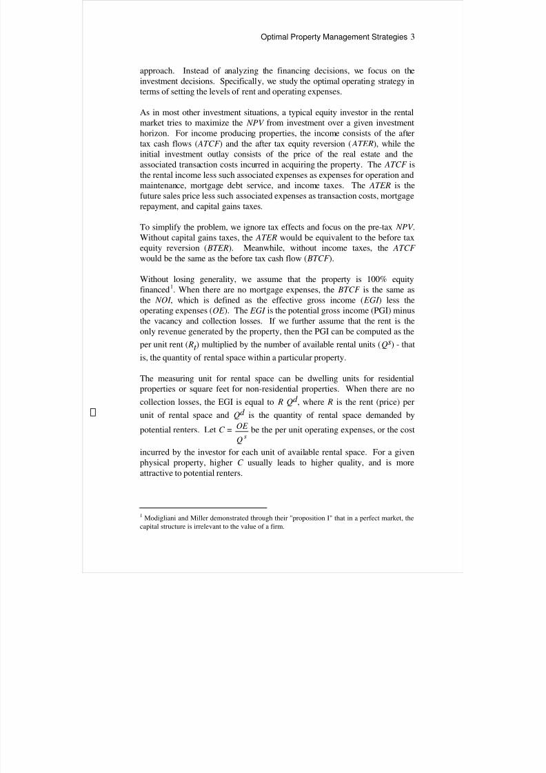
in Figure 1, the change in operating expenses corresponds to a shift in thedemand curve, while the change in rent corresponds to a move along thedemand curve. Given a specific physical property, the quality of the housing
services of each physical rental unit (apartment or house) increases with thediscretional expenses landlords spend to maintain the property and provideextra amenities. Thus, holding rent constant, higher amenities usually lead tohigher demand. As a result, the demand curve shifts out with the operatingexpenses. This is illustrated in Figure 1, when OE increases, and the demandcurve shifts out from the solid curve to the dashed curve. On the other hand,holding operating expenses or the quality of a property constant, if rent levelwas very high, one would expect that decreasing the rent marginally wouldattract higher demand. This represents a move along the demand curve inFigure 1.
8/6/2019 Optimal Property Management Strategies_Research
http://slidepdf.com/reader/full/optimal-property-management-strategiesresearch 5/25
Optimal Property Management Strategies 5
Figure 1 The Demand Curve of a Rental Property
These behaviors lead to the following properties of the demand curve withrespect to R and C :
>∂∂
<∂∂
.0
,0
t
d t
d
C
Q
R
Q
t
t
(2)
Assuming that the demand function is independent of time, all the timesubscript in the demand function can be dropped from Equation (1).Furthermore, assuming that the real estate transaction market isinformationally efficient, real property must be sold at a price equal to the
R2
R1
R*
Rent
Q1s
Qd*
Q2s
QualityImprovement
Quantity
8/6/2019 Optimal Property Management Strategies_Research
http://slidepdf.com/reader/full/optimal-property-management-strategiesresearch 6/25
6 Colwell, Kung and Yang
maximum present value of the future NOI 's2. According to Gordon's rule, thevalue of an investment is the future potential income discounted by theinvestor's required return. Every investor who is interested in purchasing theproperty will operate the property so as to maximize his NPV from theinvestment. When the market is informationally efficient, the winner of thebid for the property at time T must pay a price equal to the maximized
present value of the NOI he is able to obtain from the property. Thus, thefuture sales price, PT , should be the maximized present value of the NOI
discounted by the cost of capital, i.
PT = Max R,C ∑∞
+=
+
−
1 )1(T t t
sd
i
CQ RQ (3)
s.t. Qd ≤ Qs.
Substituting Equation (3) into equation (1), the objective function becomes:
Max R,C
∑
∞
=
+
−
1 )1(t t
sd
i
CQ RQ- P0 =
i
CQ RQ sd −- P0 (4)
s.t. Qd ≤ Qs.
Because P0 is a fixed amount of sunk cost and i is exogenously determinedby the investor’s cost of capital, they are irrelevant to the maximizationproblem of Equation (4). Solving Equation (4) is equivalent to solvingEquation (5):
Max R,C R Qd - C Qs (5)
s.t. Qd - Qs ≤ 0.
Note that Equation (5) is nothing more than the maximization of a single
period's NOI . Under the assumption of a time-independent demand curve,the multiple period model collapses into a single period condition. Investorswould act as if they were myopic.
2 Evans (1991) discussed the meaning of market value and whether market or investment value
represents "real" value. In a soft real estate market, there are not many owners willing to sell at
these lower prices, so in effect, there are not two parties to the assumed transactions. As aresult, one has liquidation values being presented by appraisers in the guise of market values.
In such a case, the informationally efficient real estate transaction market assumption would no
longer be valid.
8/6/2019 Optimal Property Management Strategies_Research
http://slidepdf.com/reader/full/optimal-property-management-strategiesresearch 7/25
Optimal Property Management Strategies 7
Denote the optimal solutions as R* and C
*, as they can be used in computingthe optimal levels for the ratios commonly used in the real estate leasingindustry. First, the optimal vacancy rate can be computed as:
s
d
s
d s
Q
C RQ
Q
QQV
],[1
**** −=
−= . (6)
In reality, if the demand for rental space is high enough, this rate can bebrought down to zero. Figure 1 shows that having a zero vacancy rate may ormay not be the optimal strategy. Suppose the unconstrained optimal quantity
to be leased is Qd * with R*. If the supply is smaller than this Qd *, such as
sQ1 in Figure 1, the constraint is binding. The manager can increase the rent
to R1 and still maintain a zero vacancy rate; yielding a higher NOI . On the
other hand, if supply were greater than Qd *, such ass
Q2 in Figure 1, then the
optimal vacancy rate would be greater than zero, but the profitability alsodecreases. This is consistent with Colwell’s (1991) finding. Of course, bylowering the rent to R2, the manager could bring the vacancy rate down to
zero.
Two other popular operating ratios referred to in the industry are the IncomeRatio ( IR) and the Operating Expense Ratio (OER). Their optimal levelsunder this framework are:
IR* =*
*
PGI
NOI =
s
sd
Q R
QC C RQ R
*
**** ],[ − , and (7)
OER* =*
*
EGI
OE =
],[ ***
*
C RQ R
QC
d
s. (8)
Again, whether the result of Equation (8) is consistent with the rule of thumb
is hard to determine. The example provided in the next section suggests thatthe rule of thumb fails to provide a unique operating strategy.
A Specific Solution
A Cobb-Douglas demand function is used to give a more precise sense of how the above optimal strategies work. The specific form of the demandcurve we choose is:
8/6/2019 Optimal Property Management Strategies_Research
http://slidepdf.com/reader/full/optimal-property-management-strategiesresearch 8/25
8 Colwell, Kung and Yang
Qd =δ
β
α C
RQ −0 , (9)
where Q0 is the total potential demand for rental space if no rent isrequired,α is a scalar that measures the effect of operating strategy on the
quantity of rental space demanded,
β =d
d
RQQ
Q
−0ε is a measure of rent elasticity of demand ( Rε is the rent
elasticity of demand),
δ =d
d
C QQ
Q
−−
0ε is a measure of operating expense elasticity of demand
( C ε is the operating expense elasticity of demand), and
δ β α ,,,0Q > 0.
This Cobb-Douglas demand curve is a flexible and reasonable functionalform to capture the local behavior of the demand curve. The local concavitybehavior is applicable to a wide range of demand curves that satisfy theproperties in Equation (2). In particular, we have:
>=∂∂
<−=∂∂
+
−
.0
,0
1
1
δ
β
δ
β
αδ
αβ
C
R
R
Q
C
R
R
Q
d
d
(10)
Substituting this demand function into Equation (5), we are able to solve forthe optimal level of rent and operating expense, and to obtain insight into thevalidity of the rules of thumb. Because of the existence of the inequalityconstraint, the problem can be solved for two conditions: 1) the constraint isnot binding; and 2) the constraint is binding.
Constraint not binding
When the constraint is not binding, the first order necessary conditions forthe optimization problem are:
=−=∂
∂
=+−=∂
∂
+
+.0
,0)1(
1
1
0
sQC
R
C
NOI
and C
RQ
R
NOI
δ
β
δ
β
αδ
β α (11)
8/6/2019 Optimal Property Management Strategies_Research
http://slidepdf.com/reader/full/optimal-property-management-strategiesresearch 9/25
Optimal Property Management Strategies 9
Solving the simultaneous Equation (11), the optimal rent and optimaloperating expense are found to be:
+=
+=
−
+
−
+
+
+
.
)1(
and,
)1() /(1
1
0*
) /(1
1
0*
1
1
δ β
β
β δ
δ β
δ
δ δ
β α
β α
β
β
δ
δ
s
s
Q
QC
Q
Q R
(12)
To make sure that this solution is indeed the maximum instead of a minimumor a saddle point, we double-check the second order conditions. The three-second order partial derivatives for the NOI are:
+=∂∂
<+−=∂
<+−=∂
+∂
++∂
−∂
.)1(
,0)1(
,0)1(
1
2
21
22
1
2
2
δ
β
δ β
δ
β
β αδ
δ αδ
β αβ
C
R
C R
NOI
and C
R
C
NOI
C
R
R
NOI
(13)
The first two of these second order partial derivatives carry negative signs,and thereby guarantee that the solution set is not a minimum. To ensure thatthe solution is not a saddle point, the necessary condition for the solution tosatisfy is :
22
2
2
2
2
∂∂−
∂
∂
∂∂∂
C C
NOI
C
NOI
R
NOI = β - δ > 0. (14)
This result indicates that δ β > is the only additional requirement to ensure
the Equation (12) solution set is the maximum.Plugging Equation (12) into Equation (9), we find the optimal quantitydemand to be:
Qd * = Q0 β
β
+1> 0. (15)
Recall that the solution set we computed above is for the case in which the
constraint is not binding. For this solution to be an interior solution, Qd *
8/6/2019 Optimal Property Management Strategies_Research
http://slidepdf.com/reader/full/optimal-property-management-strategiesresearch 10/25
10 Colwell, Kung and Yang
must be smaller than the quantity supplied. This is the same as requiring Qs
≥ β
β
+1Q0. The optimal NOI the landlord obtains by using the optimal
strategy ( R*,C *) is found to be:
NOI * =
)(1
1
1
0
)1(
)(δ β
δ
β
β
δ δ
β α
δ β −+
+−
+sQ
Q . (16)
Since δ β > , the NOI * is always greater than zero. This result ensures that
the solution set is not dominated by the trivial solution that R = C = 0.Substituting the solution set into Equations (6), (7), and (8), we find theoperating ratios indicated by the strategy of maximizing the net operatingincome:
=
+
−=
+
−=
.
and,)1(
)(
,
)1(
1
*
0*
0*
β
δ β
δ β β
β
OER
Q
Q IR
Q
QV
s
s
(17)
These optimal ratios demonstrate several interesting points. First, V *, theoptimal vacancy rate is always smaller than or equal to 100 percent becausethe second term of the first line of Equation (17) is always positive. On theother hand, because the physical constraint is not binding, the quantity
demanded must be smaller than Qs. Therefore, for the solution set to be themaximum with the constraint not binding, the quantity of space supplied mustbe greater than the quantity demanded. This criterion prevents the secondterm in the first line of Equation (17) from being greater than 1. That is, the
V * is greater than 0. Otherwise, it belongs to the case where the constraint isbinding. For a given market condition, a larger building is more likely torealize an interior solution. Satisfying this criterion is equivalent to sayingthat the optimal vacancy rate is strictly greater than zero. A zero vacancyrate fails to provide the maximum possible profit. By merely increasing therent level, the landlord can increase the NOI . When the operating expense isadjusted simultaneously, the NOI can be brought to an even higher level.
Second, the income ratio is also between 0 and 1. The relationship β > δ ,which we obtained from Equation (14), guarantees this income ratio to be
8/6/2019 Optimal Property Management Strategies_Research
http://slidepdf.com/reader/full/optimal-property-management-strategiesresearch 11/25
Optimal Property Management Strategies 11
positive. Also, since)1(
)(
)1(
00
β
δ β
β
β
+−
>+
> QQQ
s , the IR* is always less than
1. Finally, the operating expense ratio is always between 0 and 1. It is
obvious that this ratio can never be negative, and given that β > δ , the OER*
is always smaller than 1.
Constraint Binding
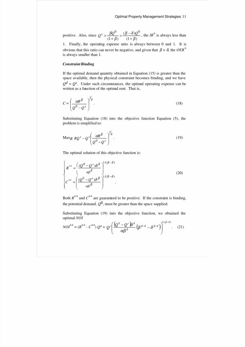
If the optimal demand quantity obtained in Equation (15) is greater than thespace available, then the physical constraint becomes binding, and we have
Qd = Qs. Under such circumstances, the optimal operating expense can bewritten as a function of the optimal rent. That is,
C =δ β α
1
0
− sQQ
R . (18)
Substituting Equation (18) into the objective function Equation (5), the
problem is simplified to:
Max R δ β α
1
0
−−
s
ss
RQ RQ . (19)
The optimal solution of this objective function is:
−=
−=
−
−
.)(
)(
) /(10
**
) /(10
**
δ β
β αβ
β
δ β
δ αβ
δ
δ
δ
s
s
QQC
QQ R
(20)
Both R** and C ** are guaranteed to be positive. If the constraint is binding,
the potential demand, Q0, must be greater than the space supplied.
Substituting Equation (19) into the objective function, we obtained theoptimal NOI
NOI ** = ( R** - C **) Qs =( ) ( )
) /(10
δ β
δ β δ β
β
δ
δ β αβ
δ −
−−
−
− ss QQ
Q . (21)
8/6/2019 Optimal Property Management Strategies_Research
http://slidepdf.com/reader/full/optimal-property-management-strategiesresearch 12/25
12 Colwell, Kung and Yang
This NOI ** is greater than zero because β is greater than δ . Therefore,Equation (21) guarantees the existence of a non-trivial solution.Furthermore, since the constraint is binding, increasing the building sizemarginally implies an increase in NOI . The positive signs on the comparativestatics introduced in the next section confirm this result.
Since the constraint is binding, we know that the space demanded, given the( R**,C **) strategy, equals the space supplied. That is, the optimal vacancy
rate, V **, is zero. In other words, when the demand for rental space is high,
or Q0 >> Qs, maximizing NPV can be achieved by minimizing the vacancyrate.
If the constraint were binding, the quantity demanded would be equal to the
quantity supplied. This condition simplifies the income ratio to be R
C −1 and
the operating expense ratio to be R
C . Substituting Equation (20) into R and
C above, we get:
=
−=
.
,1
**
**
β
δ β
δ
OER
and IR(22)
A constrained condition can be used to explain markets with rent control. Inthose markets, the rent elasticity is less than one, meaning the landlord canincrease NOI by increase rent. This additional constraint leads to a zerovacancy rate. In order to increase NOI , the operating policy is to lower theoperating expenses to the minimum level. As a result, the unit of housingservices provided by each rental unit decreases. The demand curve shiftsdown. Landlords will continue this as long as it does not violate the safetycodes.
To summarize, the objective of maximizing the investor's NPV does providea unique optimal operating strategy for the given demand function. The
physical constraint is likely to be binding when Qs is much smaller than thetotal potential demand for space. The optimal strategy derived in this sectioncan help property managers achieve the highest return on investments.
8/6/2019 Optimal Property Management Strategies_Research
http://slidepdf.com/reader/full/optimal-property-management-strategiesresearch 13/25
Optimal Property Management Strategies 13
Comparative statics
In addition to the optimal operating strategy, investors may also be interested
in the impacts of changes in market conditions (i.e. changes in Q0, Qs,
δ β α and,, ) on the profit maximization rent/expense combinations across
sub-markets or over time. These impacts are analyzed by the comparativestatics. Table 1 presents the signs of all the comparative statics for the NPV
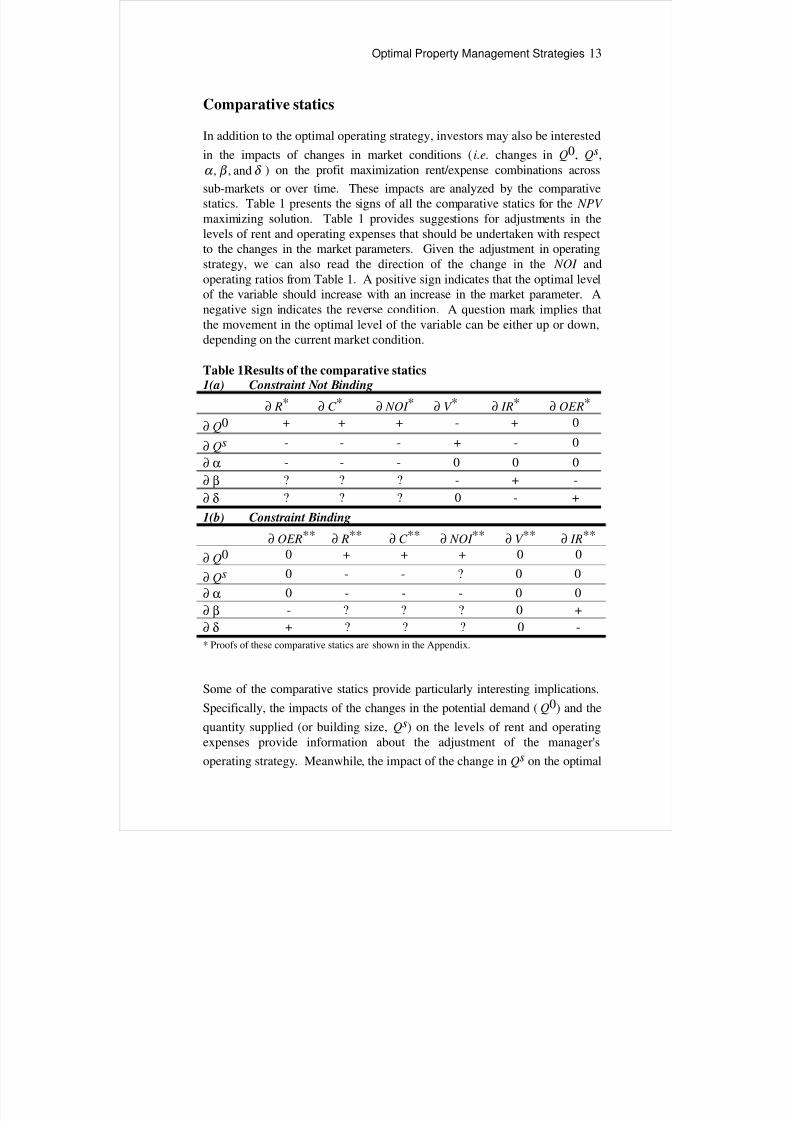
maximizing solution. Table 1 provides suggestions for adjustments in thelevels of rent and operating expenses that should be undertaken with respectto the changes in the market parameters. Given the adjustment in operatingstrategy, we can also read the direction of the change in the NOI andoperating ratios from Table 1. A positive sign indicates that the optimal levelof the variable should increase with an increase in the market parameter. Anegative sign indicates the reverse condition. A question mark implies thatthe movement in the optimal level of the variable can be either up or down,depending on the current market condition.
Table 1Results of the comparative statics1(a) Constraint Not Binding
∂ R* ∂ C * ∂ NOI * ∂ V * ∂ IR* ∂ OER*
∂ Q0 + + + - + 0
∂ Qs - - - + - 0
∂ α - - - 0 0 0
∂ β ? ? ? - + -
∂ δ ? ? ? 0 - +
1(b) Constraint Binding
∂ OER** ∂ R** ∂ C ** ∂ NOI ** ∂ V ** ∂ IR**
∂ Q0 0 + + + 0 0
∂ Qs 0 - - ? 0 0
∂ α 0 - - - 0 0
∂ β - ? ? ? 0 +
∂ δ + ? ? ? 0 -
* Proofs of these comparative statics are shown in the Appendix.
Some of the comparative statics provide particularly interesting implications.
Specifically, the impacts of the changes in the potential demand ( Q0) and the
quantity supplied (or building size, Qs) on the levels of rent and operatingexpenses provide information about the adjustment of the manager's
operating strategy. Meanwhile, the impact of the change in Qs on the optimal
8/6/2019 Optimal Property Management Strategies_Research
http://slidepdf.com/reader/full/optimal-property-management-strategiesresearch 14/25
14 Colwell, Kung and Yang
NOI provides some insight into the optimal development and rehabilitationstrategies.
First, a change in the quantity supplied has the same impact on the optimallevels of rent and operating expense regardless of whether the constraint isbinding. If there is an increase in the quantity of the space available for
lease, then the manager should lower the rent and cut the operating expensein order to achieve a new optimal NOI . It may sound strange that thephysical size of the real property can change. Several conditions could
induce a change in Qs. One example would be if an existing building weretorn down and replaced by a larger or smaller building. Another would bethe case in which a new building was acquired by the management team andas a result, the quantity of total space supply controlled by the same managerwas increased. Yet another case might be the conversion of owner-occupiedspace to renter-occupied space. In accordance with the change in the amountof space under control, the manager should adjust his operating strategy toachieve the new optimal NOI .
Second, an increase in the number of potential renters implies that the
manager should raise the rent and operating expenses regardless of whetherthe constraint is binding or not. In either case, the optimal NOI increases. Itis important for the manager to determine which condition he is facing inorder to make the best adjustment.
Finally, while a greater Qs implies a lower NOI when the constraint is not
binding, the change in the optimal NOI with respect to the change in Qs when
the constraint is binding is indeterminate. The negative sign of sQ
NOI
∂
∂ *in
Table 1(a) shows that a smaller building implies a higher NOI . Since our
demand function does not depend on the Qs, a decrease in Qs decreases total
costs while leaving total revenue unchanged. As a result, the NOI would behigher under such a circumstance. This result suggests that when developinga new rental building, the investor should make the building as small aspossible. However, as the building size decreases, it is more likely that thephysical constraint becomes binding. If the physical constraint holds, weshould focus on the result provided in Table 1(b). The sign of
sQ
NOI
∂
∂ **depends on the amount of space available. Specifically, the sign is
negative if and only if Qs is greater than)(1
)(0
δ β
δ β
−+−Q
, and positive if and
8/6/2019 Optimal Property Management Strategies_Research
http://slidepdf.com/reader/full/optimal-property-management-strategiesresearch 15/25
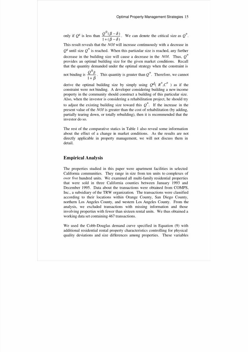
Optimal Property Management Strategies 15
only if Qs is less than)(1
)(0
δ β
δ β
−+−Q
. We can denote the critical size as Q*.
This result reveals that the NOI will increase continuously with a decrease in
Qs until size Q* is reached. When this particular size is reached, any further
decrease in the building size will cause a decrease in the NOI . Thus, Q*
provides an optimal building size for the given market conditions. Recallthat the quantity demanded under the optimal strategy when the constraint is
not binding isβ
β
+1
0Q. This quantity is greater than Q*. Therefore, we cannot
derive the optimal building size by simply using Qd ( R*,C * ) as if theconstraint were not binding. A developer considering building a new incomeproperty in the community should construct a building of this particular size.Also, when the investor is considering a rehabilitation project, he should try
to adjust the existing building size toward this Q*. If the increase in thepresent value of the NOI is greater than the cost of rehabilitation (by adding,partially tearing down, or totally rebuilding), then it is recommended that theinvestor do so.
The rest of the comparative statics in Table 1 also reveal some informationabout the effect of a change in market conditions. As the results are notdirectly applicable in property management, we will not discuss them indetail.
Empirical Analysis
The properties studied in this paper were apartment facilities in selectedCalifornia communities. They range in size from ten units to complexes of over five hundred units. We examined all multi-family residential propertiesthat were sold in three California counties between January 1993 andDecember 1995. Data about the transactions were obtained from COMPS,Inc., a subsidiary of the TRW organization. The transactions were classifiedaccording to their locations within Orange County, San Diego County,northern Los Angeles County, and western Los Angeles County. From theanalysis, we excluded transactions with missing information and thoseinvolving properties with fewer than sixteen rental units. We thus obtained aworking data set containing 467 transactions.
We used the Cobb-Douglas demand curve specified in Equation (9) withadditional residential rental property characteristics controlling for physicalquality deviations and size differences among properties. These variables
8/6/2019 Optimal Property Management Strategies_Research
http://slidepdf.com/reader/full/optimal-property-management-strategiesresearch 16/25
16 Colwell, Kung and Yang
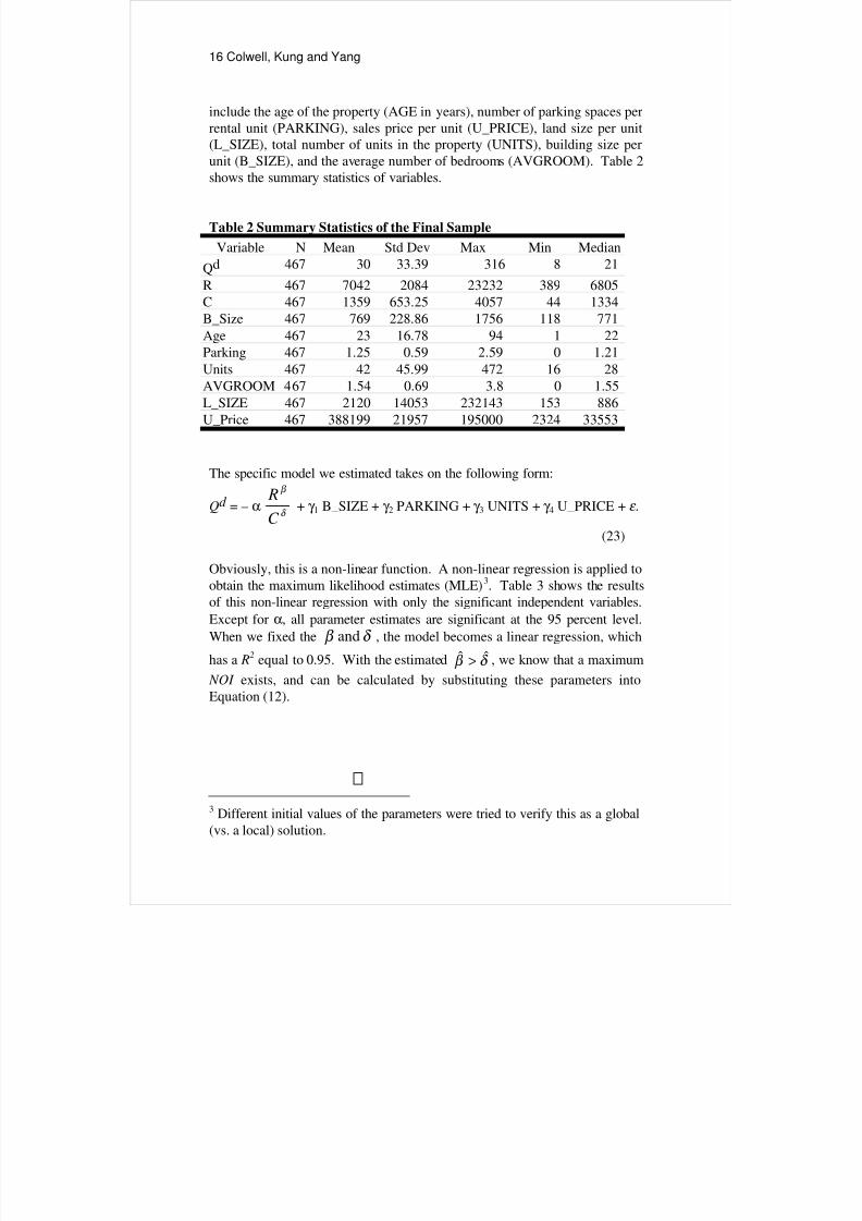
include the age of the property (AGE in years), number of parking spaces perrental unit (PARKING), sales price per unit (U_PRICE), land size per unit(L_SIZE), total number of units in the property (UNITS), building size perunit (B_SIZE), and the average number of bedrooms (AVGROOM). Table 2shows the summary statistics of variables.
Table 2 Summary Statistics of the Final Sample
Variable N Mean Std Dev Max Min Median
Qd 467 30 33.39 316 8 21
R 467 7042 2084 23232 389 6805
C 467 1359 653.25 4057 44 1334
B_Size 467 769 228.86 1756 118 771
Age 467 23 16.78 94 1 22
Parking 467 1.25 0.59 2.59 0 1.21
Units 467 42 45.99 472 16 28
AVGROOM 467 1.54 0.69 3.8 0 1.55
L_SIZE 467 2120 14053 232143 153 886
U_Price 467 388199 21957 195000 2324 33553
The specific model we estimated takes on the following form:
Qd = – α δ
β
C
R+ γ 1 B_SIZE + γ 2 PARKING + γ 3 UNITS + γ 4 U_PRICE + ε .
(23)
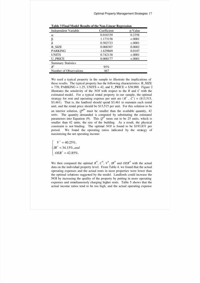
Obviously, this is a non-linear function. A non-linear regression is applied toobtain the maximum likelihood estimates (MLE)3. Table 3 shows the resultsof this non-linear regression with only the significant independent variables.
Except for α, all parameter estimates are significant at the 95 percent level.
When we fixed the δ β and , the model becomes a linear regression, whichhas a R
2 equal to 0.95. With the estimated δ β ˆˆ > , we know that a maximum
NOI exists, and can be calculated by substituting these parameters intoEquation (12).
3 Different initial values of the parameters were tried to verify this as a global(vs. a local) solution.
8/6/2019 Optimal Property Management Strategies_Research
http://slidepdf.com/reader/full/optimal-property-management-strategiesresearch 17/25
8/6/2019 Optimal Property Management Strategies_Research
http://slidepdf.com/reader/full/optimal-property-management-strategiesresearch 18/25
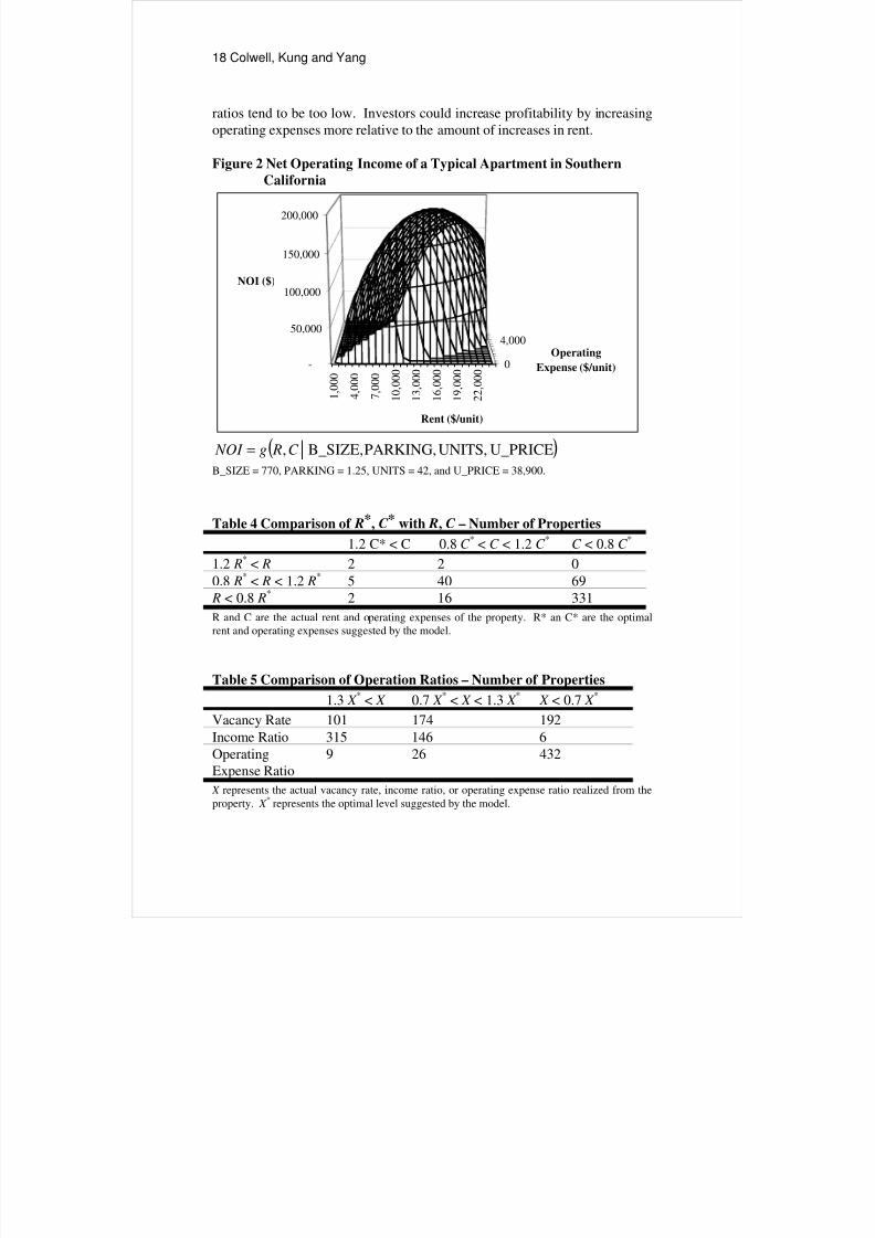
18 Colwell, Kung and Yang
ratios tend to be too low. Investors could increase profitability by increasingoperating expenses more relative to the amount of increases in rent.
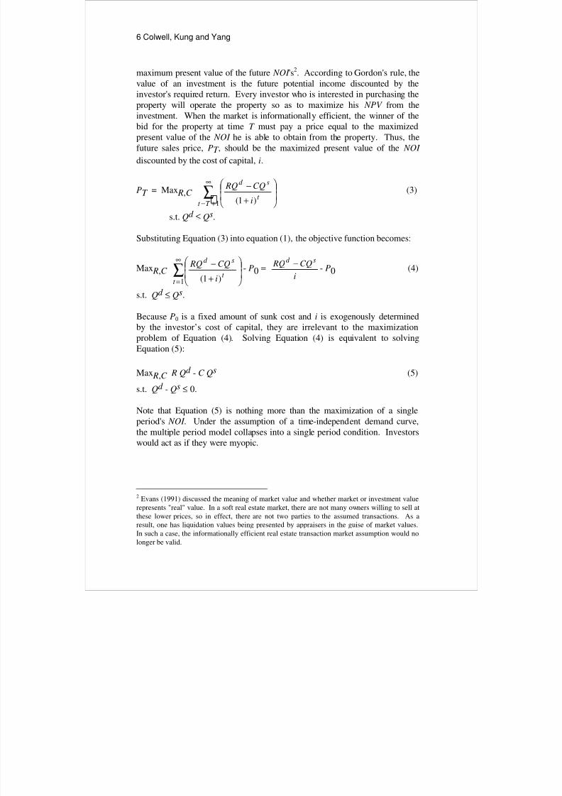
Figure 2 Net Operating Income of a Typical Apartment in SouthernCalifornia
1 ,
0 0 0
4 ,
0 0 0
7 ,
0 0 0
1 0 ,
0 0 0
1 3 ,
0 0 0
1 6 ,
0 0 0
1 9 ,
0 0 0
2 2 ,
0 0 0
0
4,000
-
50,000
100,000
150,000
200,000
NOI ($)
Rent ($/unit)
Operating
Expense ($/unit)
( )U_PRICEUNITS,PARKING,B_SIZE,,C Rg NOI =B_SIZE = 770, PARKING = 1.25, UNITS = 42, and U_PRICE = 38,900.
Table 4 Comparison of R*, C * with R, C – Number of Properties
1.2 C* < C 0.8 C * < C < 1.2 C
*C < 0.8 C
*
1.2 R* < R 2 2 0
0.8 R* < R < 1.2 R
* 5 40 69
R < 0.8 R* 2 16 331
R and C are the actual rent and operating expenses of the property. R* an C* are the optimalrent and operating expenses suggested by the model.
Table 5 Comparison of Operation Ratios – Number of Properties
1.3 X * < X 0.7 X
* < X < 1.3 X *
X < 0.7 X *
Vacancy Rate 101 174 192
Income Ratio 315 146 6
OperatingExpense Ratio
9 26 432
X represents the actual vacancy rate, income ratio, or operating expense ratio realized from the
property. X * represents the optimal level suggested by the model.
8/6/2019 Optimal Property Management Strategies_Research
http://slidepdf.com/reader/full/optimal-property-management-strategiesresearch 19/25
Optimal Property Management Strategies 19
One should notice that the sample represents a recession market. SouthernCalifornia suffered from a prolonged recession in the early 1990’s. Thevacancy rate during this time period tends to be high. Finding ways to attracttenants is a very challenging task. The data observed in this empirical studyreflects this condition. However, our model suggests that there is significantroom for most property managers to improve their performance by resetting
their pricing strategies. Sometimes, higher income ratios and lower operatingexpense ratios may not lead to maximum profitability.
Conclusions
In this paper, we showed that if the demand curve is time independent, theninvestors in rental properties are expected to behave as if they are myopic.That is, the strategy that maximizes the net present value of investment isidentical to maximizing a single period's net operating income.
With a given demand curve, one can algebraically derive the operatingstrategies in terms of setting the levels of rent and operating expenses. We
used a Cobb-Douglas demand curve to demonstrate the process and to studythe properties of such optimal strategies. The impact of changes in marketconditions on NOI over time or across sub-markets care were also revealedby comparative statics. These comparative statics also provided insights intothe adjustment that one can make corresponding to the new environment tobe maintained at the optimal position. These results also implied the idealbuilding size under a specific market. Rehabilitation could be optimal as theincrease in the present value of net operating income exceeds the costs of adjusting the building size.
Cross-sectional multi-family transaction data from southern California wasused to empirically estimate a Cobb-Douglas demand function. Based on theestimated parameters, we found that the actual operating expense and the
actual rent tend to be lower than the optimal levels suggested by the model.On the other hand, the income ratio tends to be too high and the operatingexpense ratio tends to be too low. This suggests that when setting operatingstrategies, property managers should not simply focus on one or two ratios.Sensitivity of the demand (quantity) associated with the rent (price) andoperating expense (quality) are just as important.
This model can also be used when the demand curve is estimated by timeseries data. With proprietary historical performance data, a propertymanager would be able to determine the optimal operating strategy. This isparticularly valuable to managers of short-term lease properties, such ashotels.
8/6/2019 Optimal Property Management Strategies_Research
http://slidepdf.com/reader/full/optimal-property-management-strategiesresearch 20/25
20 Colwell, Kung and Yang
References
Cannaday, R. E. and Yang, T.L. Tyler, (1995), Optimal interest rate-discountpoints combination: strategy for mortgage contract terms, Journal of the
American Real Estate and Urban Economics Association: Real Estate Economics, 23, 1, 65-83.
Cannaday, R. E. and Yang, T.L. Tyler, (1996), Optimal Leverage Strategy:Capital Structure in Real Estate Investments, Journal of Real Estate Finance
and Economics, 13, 3, 263-271.
Chinloy, Peter and Maribojoc, Eric, (1998), Expense and rent strategies inreal estate management, Journal of Real Estate Research, 15, 3, 267-282.
Colwell, Pete F., (1991), Vacancy management, Journal of Property
Management , 56, 3, 42-44.
Evans, Mariwyn, (1991), What is real estate worth?, A debate over themeaning of market value, Journal of Property Management , 56, 3, 46-48.
8/6/2019 Optimal Property Management Strategies_Research
http://slidepdf.com/reader/full/optimal-property-management-strategiesresearch 21/25
Optimal Property Management Strategies 21
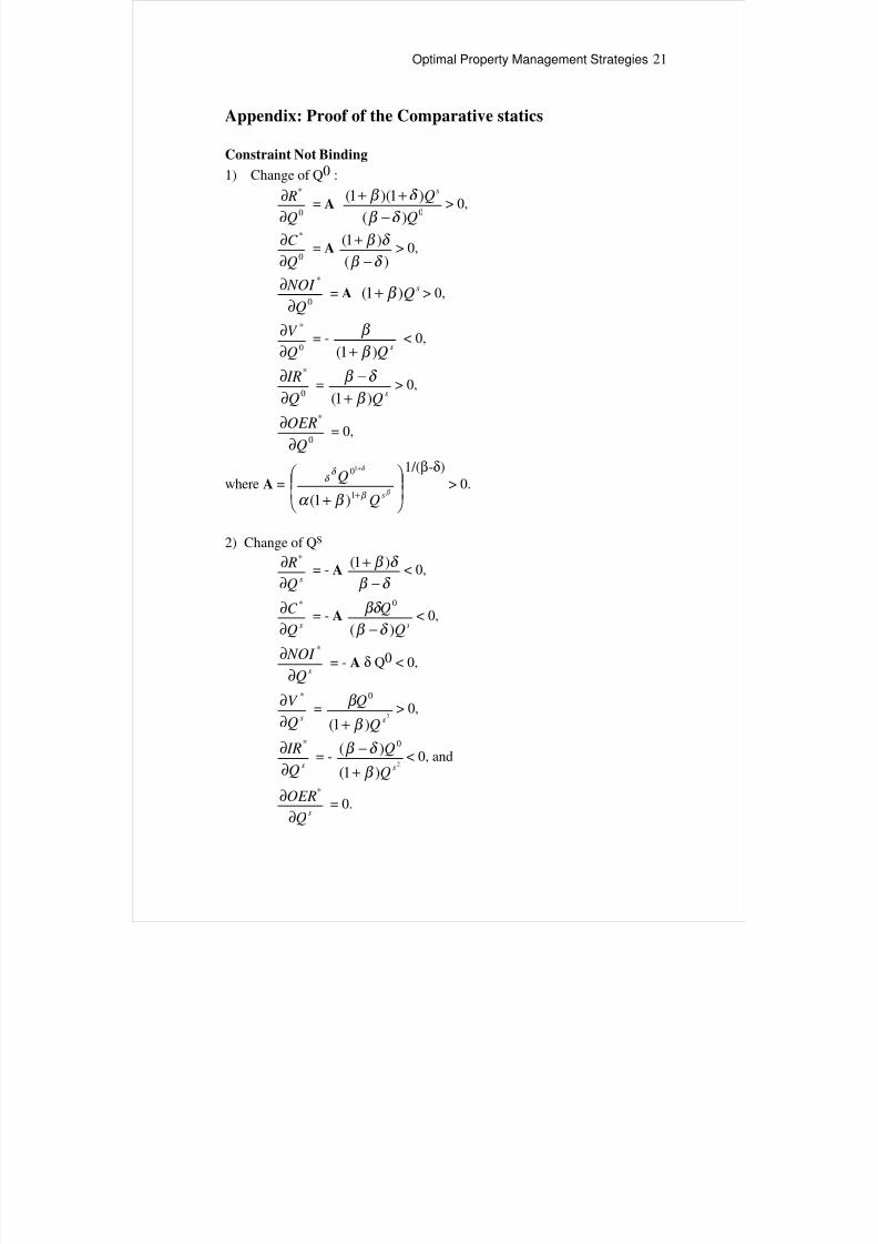
Appendix: Proof of the Comparative statics
Constraint Not Binding
1) Change of Q0 :
0
*
Q
R
∂
∂= A
0
)(
)1)(1(
Q
Qs
δ β
δ β
−
++> 0,
0
*
Q
C
∂∂
= A )(
)1(
δ β
δ β
−+
> 0,
0
*
Q
NOI
∂∂
= A s
Q)1( β + > 0,
0
*
Q
V
∂∂
= -s
Q)1( β
β
+< 0,
0
*
Q
IR
∂∂
=s
Q)1( β
δ β
+−
> 0,
0
*
Q
OER
∂∂
= 0,
where A =
+ +
+
β
δ
β
δ δ
β α sQ
Q1
0
)1(
1 1/(β-δ)
> 0.
2) Change of Qs
sQ
R
∂∂ *
= - A δ β
δ β
−+ )1(
< 0,
sQ
C
∂∂ *
= - A s
Q
Q
)(
0
δ β
βδ
−< 0,
sQ
NOI ∂
∂*
= - A δ Q0 < 0,
sQ
V
∂∂ *
=2
)1(
0
sQ
Q
β
β
+> 0,
sQ
IR
∂∂ *
= -2
)1(
)( 0
sQ
Q
β
δ β
+
−< 0, and
sQ
OER
∂∂ *
= 0.
8/6/2019 Optimal Property Management Strategies_Research
http://slidepdf.com/reader/full/optimal-property-management-strategiesresearch 22/25
22 Colwell, Kung and Yang
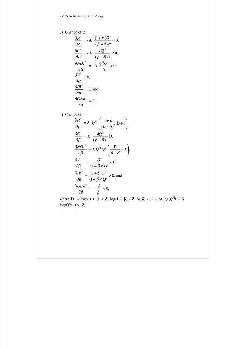
3) Change of α
α ∂∂ * R
= - A α δ β
β
)(
)1(
−+ s
Q< 0,
α ∂∂ *C
= - A α δ β
δ
)(
0
−Q
< 0,
α ∂∂ * NOI
= - A α
sQQ0
< 0,
α ∂∂ *V
= 0,
α ∂∂ * IR
= 0, and
α ∂∂ *OER
= 0.
4) Change of β
β ∂∂*
R = A Qs +−+ 1)(
1 2 Dδ β β ,
β ∂∂ *C
= A 2
0
)( δ β
δ
−Q
D,
β ∂∂ * NOI
= A Q0 Qs
+
−2
δ β
D,
β ∂∂ *V
= -sQ
Q2
0
)1( β +< 0,
β ∂∂ * IR
=sQ
Q2
0
)1(
)1(
β
δ
++
> 0, and
β ∂∂ *OER
= -2β
δ < 0,
where D = log(α) + (1 + δ) log(1 + β) - δ log(δ) - (1 + δ) log(Q0) + δlog(Qs) - (β - δ)
8/6/2019 Optimal Property Management Strategies_Research
http://slidepdf.com/reader/full/optimal-property-management-strategiesresearch 23/25
Optimal Property Management Strategies 23
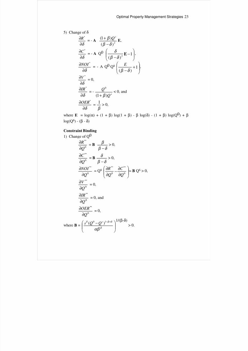
5) Change of δ
δ ∂∂ * R
= - A 2)(
)1(
δ β
β
−+ sQ
E,
δ ∂∂ *C
= - A Q0
−
−1
)( 2E
δ β
δ ,
δ ∂∂ * NOI
= - A Q0 Qs
+
−1
)( δ β
E ,
δ ∂∂ *V
= 0,
δ ∂∂ * IR
= -sQ
Q
)1(
0
β +< 0, and
δ ∂∂ *OER
=β
1> 0,
where E = log(α) + (1 + β) log(1 + β) - β log(δ) - (1 + β) log(Q0) + β
log(Qs) - (β - δ)
Constraint Binding
1) Change of Q0
0
**
Q
R
∂∂
= B δ β
β
−> 0,
0
**
Q
C
∂∂
= B δ β
δ
−> 0,
0
**
Q
NOI
∂∂
= Qs
∂∂
−∂∂
0
**
0
**
Q
C
Q
R= B Qs > 0,
0
**
Q
V
∂∂ = 0,
0
**
Q
IR
∂∂
= 0, and
0
**
Q
OER
∂∂
= 0,
where B =
− +−
β
δ β δ δ
αβ
10 )( sQQ
1/(β-δ)
> 0.
8/6/2019 Optimal Property Management Strategies_Research
http://slidepdf.com/reader/full/optimal-property-management-strategiesresearch 24/25
24 Colwell, Kung and Yang
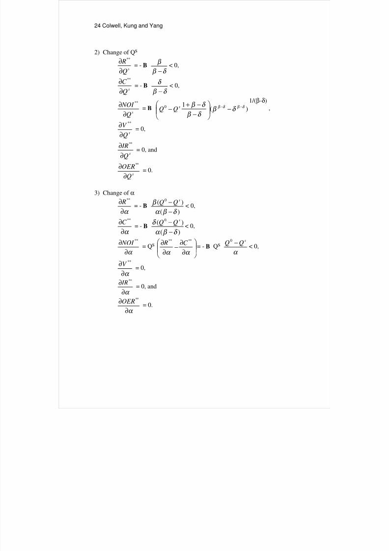
2) Change of Qs
sQ
R
∂∂ **
= - B δ β
β
−< 0,
sQ
C
∂∂ **
= - B δ β
δ
−< 0,
sQ
NOI
∂∂ **
= B )(10 δ β δ β δ β
δ β
δ β −− −
−−+
− sQQ
1/(β-δ)
,
sQ
V
∂∂ **
= 0,
sQ
IR
∂∂ **
= 0, and
sQ
OER
∂∂ **
= 0.
3) Change of α
α ∂∂ ** R
= - B )(
)( 0
δ β α
β
−− s
QQ< 0,
α ∂∂ **C
= - B )(
)( 0
δ β α
δ
−− s
QQ< 0,
α ∂∂ ** NOI
= Qs
∂∂
−∂∂
α α
**** C R= - B Qs
α
sQQ −0
< 0,
α ∂∂ **V
= 0,
α ∂
∂ ** IR
= 0, and
α ∂∂ **OER
= 0.
8/6/2019 Optimal Property Management Strategies_Research
http://slidepdf.com/reader/full/optimal-property-management-strategiesresearch 25/25
Optimal Property Management Strategies 25
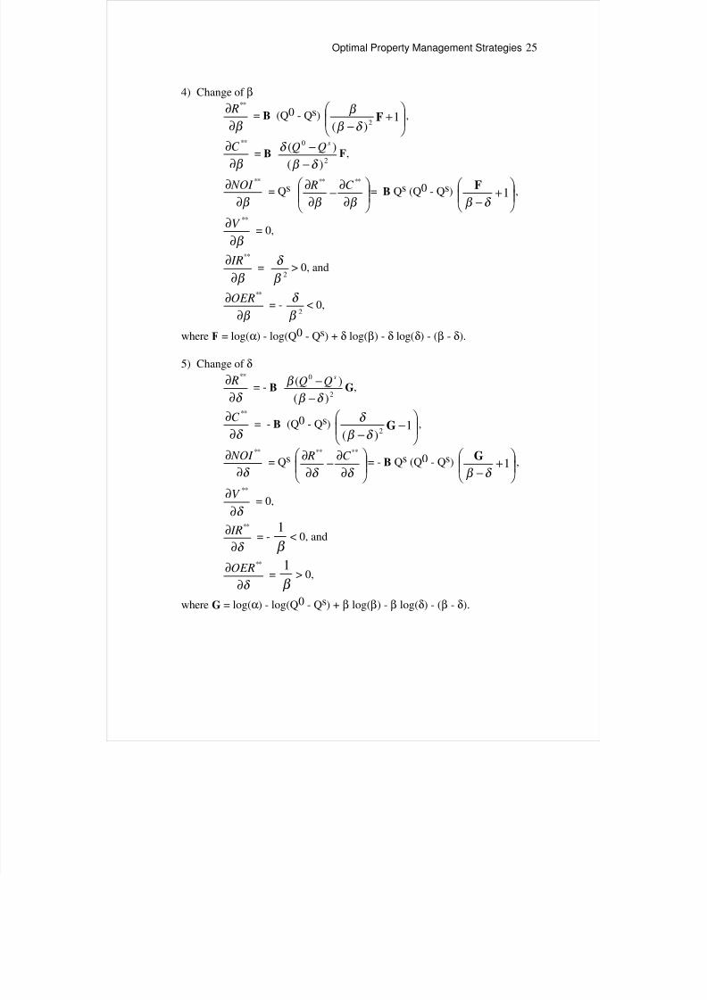
4) Change of β
β ∂∂ ** R
= B (Q0 - Qs)
+
−1
)( 2F
δ β
β ,
β ∂∂ **C
= B 2
0
)(
)(
δ β
δ
−− sQQ
F,
β ∂∂ ** NOI
= Qs
∂∂
−∂∂
β β
**** C R= B Qs (Q0 - Qs)
+
−1
δ β
F,
β ∂∂ **V
= 0,
β ∂∂ ** IR
=2β
δ > 0, and
β ∂∂ **OER
= -2β
δ < 0,
where F = log(α) - log(Q0 - Qs) + δ log(β) - δ log(δ) - (β - δ).
5) Change of δ
δ ∂∂ ** R
= - B 2
0
)(
)(
δ β
β
−− s
QQG,
δ ∂∂ **C
= - B (Q0 - Qs)
−
−1
)( 2G
δ β
δ ,
δ ∂∂ ** NOI
= Qs
∂∂
−∂∂
δ δ
**** C R= - B Qs (Q0 - Qs)
+
−1
δ β
G,
δ ∂∂ **V
= 0,
δ ∂∂ ** IR
= -β 1 < 0, and
δ ∂∂ **OER
=β
1> 0,
where G = log(α) - log(Q0 - Qs) + β log(β) - β log(δ) - (β - δ).