PHYSICAL REVIEW A 90, 033628 (2014)

Optimal quantum control of Bose-Einstein condensates in magnetic microtraps: Comparison ofgradient-ascent-pulse-engineering and Krotov optimization schemes

Georg Jager,1 Daniel M. Reich,2 Michael H. Goerz,2 Christiane P. Koch,2 and Ulrich Hohenester1

1Institut fur Physik, Karl-Franzens-Universitat Graz, Universitatsplatz 5, 8010 Graz, Austria2Theoretische Physik, Universitat Kassel, Heinrich-Plett-Str. 40, 34132 Kassel, Germany

(Received 11 August 2014; published 25 September 2014)

We study optimal quantum control of the dynamics of trapped Bose-Einstein condensates: The targets areto split a condensate, residing initially in a single well, into a double well, without inducing excitation, andto excite a condensate from the ground state to the first-excited state of a single well. The condensate isdescribed in the mean-field approximation of the Gross-Pitaevskii equation. We compare two optimizationapproaches in terms of their performance and ease of use; namely, gradient-ascent pulse engineering (GRAPE)and Krotov’s method. Both approaches are derived from the variational principle but differ in the way thecontrol is updated, additional costs are accounted for, and second-order-derivative information can be included.We find that GRAPE produces smoother control fields and works in a black-box manner, whereas Krotovwith a suitably chosen step-size parameter converges faster but can produce sharp features in the controlfields.

DOI: 10.1103/PhysRevA.90.033628 PACS number(s): 03.75.−b, 37.25.+k, 02.30.Yy

I. INTRODUCTION

Controlling complex quantum dynamics is a recurringtheme in many different areas of atomic, molecular, and optical(AMO) physics and physical chemistry. Recent examplesinclude quantum state preparation [1,2], interferometry [3]and imaging [4,5], or reaction control [6,7]. The central ideaof quantum control is to employ external fields to steer thedynamics in a desired way [8,9]. The fields that realize thedesired dynamics can be determined by optimal control theory(OCT) [10,11]. An expectation value that encodes the targetis then taken to be a functional of the external field which isminimized or maximized. The target can be simply a desiredfinal state [10] or a unitary operator [12], a prescribed valueof energy or position [13], or an experimental signal such as apump-probe trace [14].

The algorithms that can be employed for optimizing thetarget functional broadly fall into two categories—those wherechanges in the field are determined solely by evaluatingthe functional, such as simplex algorithms [13,15], and thosethat utilize derivative information, such as Krotov’s method[16,17] or gradient-ascent pulse engineering (GRAPE) [18],possibly combined with quasi-Newton methods [19,20]. Thesolutions that one obtains typically depend not only on thetarget functional but also on the specific algorithm that isemployed and the initial-guess field. This is due to the fact thatnumerical optimization is always a local search which may findone of possibly many optimal solutions or get stuck in a localextremum. It is thus important to understand which featuresof an optimal control solution are due to the optimizationprocedure and which reflect truly physical properties of thequantum system.

For example, when seeking to identify, by use of optimalcontrol theory, the quantum speed limit, i.e., the shortestpossible time in which a quantum operation can be carriedout [21], the answer should be independent of the algorithm.Moreover, in view of employing calculated solutions in anexperiment, conditions such as limited power, limited timeresolution, or limited bandwidth need to be met. The way in

which the various optimization approaches can accommodatesuch requirements differ greatly.

Here, we study control of a Bose-Einstein condensate in amagnetic microtrap, comparing several variants of a GRAPE-type algorithm [22,23] with Krotov’s method [16,17,24]. Weconsider two targets—splitting the condensate, which residesinitially in the ground state of a single well, into a double well,without inducing excitation, and exciting the condensate fromthe ground to the first-excited state of a single well. The latteris important for stimulated processes in matter waves, whereasthe former presents a crucial step in interferometry [25–27].A challenging aspect of controlling a condensate is thenonlinearity of the equation of motion which can compromiseor even prevent convergence of the optimization [17]. Thetwo methods tackle this problem in different ways: GRAPEby computing the search direction for new control fieldswithin the framework of Lagrange parameters and submittingthe optimal control search to generic minimization routines[22,28], Krotov’s method by accounting for the nonlinearityof the equations of motion in the monotonicity conditionswhen constructing the algorithm [16,17,24]. Furthermore, themethods differ in the way in which additional requirementssuch as smoothness of the control can be accounted for. Wecompare the two optimization approaches with respect to thesolutions they yield as well as their performance and ease ofuse. Our study extends an earlier comparison of GRAPE-typealgorithms with Krotov’s method [19] that was concerned withthe linear Schrodinger equation and with finite-size (spin-type)quantum systems.

Our paper is organized as follows: After introducing theequation of motion for the condensate dynamics togetherwith the control targets in Sec. II, we briefly review the twooptimization schemes in Sec. III. Section IV presents ourresults for wave-function splitting and shaking. Moreover, weinvestigate the influence of the nonlinearity, the performanceof the two algorithms, and the smoothness of the optimizedcontrol in Secs. IV B to IV D. Our conclusions are presentedin Sec. V.

1050-2947/2014/90(3)/033628(9) 033628-1 ©2014 American Physical Society

JAGER, REICH, GOERZ, KOCH, AND HOHENESTER PHYSICAL REVIEW A 90, 033628 (2014)

II. MODEL AND OPTIMIZATION PROBLEM

In this paper we consider a quasi-one-dimensional (quasi-1D) condensate residing in a magnetic confinement potentialV (x,λ(t)) that can be controlled by some external controlparameter λ(t) [2,22,23,29]. We describe the condensatedynamics within the mean-field framework of the Gross-Pitaevskii equation, where ψ(x,t) is the condensate wavefunction, normalized to one, whose time evolution is governedby [30] (� = 1)

i∂ψ (x,t)

∂t=

[− 1

2M

∂2

∂x2+ V (x,λ (t) ) + κ|ψ (x,t) |2

]×ψ (x,t) . (1)

The first term on the right-hand side is the operator for thekinetic energy, the second one is the confinement potential,and the last term is the nonlinear atom-atom interaction inthe mean-field approximation. M is the atom mass and κ isthe strength of the nonlinear atom-atom interactions, whichis related to the effective one-dimensional interaction strengthU0 and the number of atoms N through κ = U0(N − 1) [31].

We can now formulate our optimal control problem.Suppose that the condensate is initially described by the wavefunction ψ(x,0) = ψ0(x) and the potential is varied in thetime interval [0,T ]. We are now seeking for an optimal timevariation of λ(t) that brings the terminal wave function ψ(x,T )as close as possible to a desired wave function ψd (x). To ratethe success for a given control, we introduce the cost function

JT (ψ(T )) = 12 [1 − |〈ψd |ψ(T )〉|2], (2)

which becomes zero when the terminal wave function matchesthe desired one up to an arbitrary phase. Optimal control theoryaims at a λOCT(t) that minimizes Eq. (2).

III. OPTIMIZATION METHODS

In this paper, we apply two different optimal-controlapproaches; namely, a gradient-ascent-pulse-engineering(GRAPE) scheme [18] and Krotov’s method [16,17,24], whichis discussed separately below. An overview of the controlapproaches is given in Table I.

A. GRAPE: Functional and optimization scheme

The GRAPE scheme for Bose-Einstein condensates hasbeen presented in detail elsewhere [22,23,29,32], for this

reason we only briefly introduce the working equations.Experimentally, strong variations of the control parameter aredifficult to achieve. Therefore, we add to the cost function anadditional term [22,33,34],

J (ψ(T ),λ) = JT (ψ(T )) + γ

2

∫ T

0[λ(t)]2dt. (3)

Mathematically, the additional term penalizes strong variationsof the control parameter and is needed to make the OCTproblem well posed [22,33,34]. Through γ it is possible toweight the relative importance of wave-function matchingand control smoothness. Below, we set γ � 1 such that J

is dominated by the terminal cost JT .In order to bring the system from the initial state ψ0 to

the terminal state ψ(T ) we have to fulfill the Gross-Pitaevskiiequation, which enters as a constraint in our optimizationproblem. The constrained optimization problem can be turnedinto an unconstrained one by means of Lagrange multipliersp(x,t), whose time evolution is governed by [22]

ip =(

− 1

2M

∂2

∂x2+ V (x,λ(t)) + 2κ|ψ |2

)p + κψ2p∗, (4)

subject to the terminal condition p(T ) = i〈ψd |ψ(T )〉ψd . Theoptimal control problem is then composed of the Gross-Pitaevskii equation (1) and Eq. (4), which must be fulfilledsimultaneously together with [22]

γ λ = −Re〈p|∂V

∂λ|ψ〉 (5)

for the optimal control. This expression differs from standardGRAPE [18] and results from minimizing changes in thecontrol; cf. Eq. (3).

This set of equations can be also employed for a nonoptimalcontrol where Eq. (5) is not fulfilled. In this case Eq. (1) issolved forwards in time and Eq. (4) backwards in time, andthe search direction ∇λJ for an improved control is calculatedfrom one of the Eqs. [22,23,34]:

∇λJ = −γ λ − Re〈p|∂V

∂λ|ψ〉 for L2 norm, (6)

− d2

dt2[∇λJ ] = −γ λ − Re〈p|∂V

∂λ|ψ〉 for H 1 norm. (7)

These two expressions are obtained by interpreting, on theright-hand side of Eq. (3), the integral

∫ T

0 [λ]2dt = 〈λ,λ〉L2 =〈λ,λ〉H 1 in terms of an L2 or H 1 norm [31,34]. The H 1 norm

TABLE I. Optimization approaches used in this paper. For each algorithm, we specify whether a line search is used, which free parameteris available to influence the optimization, the order of the derivative for the determination of the new control parameter, the penalty term thatis added to Eq. (2), with �λ = λ − λref , the equation for the cost function, the type of the update of the control, and the update equation usedin our simulations.

Line Free Penalty UpdateAlgorithm search parameter Deriv. Penalty equation Update equation

GRAPE grad L2 Yes γ 1 λ2 Eq. (3) Concurrent Eq. (6)GRAPE grad H1 Yes γ 1 λ2 Eq. (3) Concurrent Eq. (7)GRAPE BFGS L2 Yes γ 2 λ2 Eq. (3) Concurrent Eq. (6)GRAPE BFGS H1 Yes γ 2 λ2 Eq. (3) Concurrent Eq. (7)Krotov No k 1 (�λ)2 Eq. (9) Sequential Eq. (10)KBFGS No k 2 (�λ)2 Eq. (9) Sequential Eq. (38) of Ref. [20]

033628-2

OPTIMAL QUANTUM CONTROL OF BOSE-EINSTEIN . . . PHYSICAL REVIEW A 90, 033628 (2014)

implies that one additionally has to solve a Poisson equation;see the derivative operator on the left-hand side of Eq. (7). Thisgenerally results in a much smoother time dependence of thecontrol parameters while the additional numerical effort forsolving the Poisson equation is negligible. As for an optimalcontrol, both Eqs. (6) and (7) yield ∇λJ = 0.

Here we solve the optimal control equations using theMatlab toolbox OCTBEC [23]. The ground and desired statesof the Gross-Pitaevskii equation are computed by using theoptimal damping algorithm [23,35]. The control parametersare obtained iteratively by using either a conjugate gradientmethod (GRAPE grad), which only uses first-order informa-tion, or a quasi-Newton Broyden-Fletcher-Goldfarb-Shanno(BFGS) scheme [36] (GRAPE BFGS), which also takesinto account second-order information via an approximatedHessian. In both cases, the optimization employs a line searchto determine the optimal step size in the direction of a givengradient. The pulse update is calculated for all time pointssimultaneously, making the GRAPE schemes concurrent.

B. Krotov’s method: Functional and optimization scheme

Krotov’s method [16] provides an alternative optimalcontrol implementation. The main idea is to add to Eq. (2)a vanishing term [16,17,24], which is chosen such that theminimum of the new function is also a minimum of J .However, for nonoptimal λ(t) one can devise a scheme thatalways gives a new control corresponding to a lower costfunction. Thus, Krotov’s method leads to a monotonicallyconvergent optimization algorithm that is expected to exhibitmuch faster convergence.

Our implementation closely follows Refs. [17,20,24].Specifically, the cost reads

J (ψ(T ),λ) = JT (ψ(T )) +∫ T

0

[λ (t) − λref (t)]2

S (t)dt, (8)

where the reference field λref(t) is typically chosen to be thecontrol from the previous iteration [37]. The second term inEq. (8) penalizes changes in the control from one iteration tothe next and ensures that, as an optimum is approached, thevalue of the functional is increasingly determined by only JT .S(t) = ks(t) is a shape function that controls the turning onand off of the control fields, k is a step-size parameter, ands(t) ∈ [0,1] is bound between 0 and 1.

Let ψ (i)(t) and λ(i)(t) denote the wave function and controlparameter, respectively, in the ith iteration of the optimalcontrol loop. To get started, we first solve for an initialguess λ(0)(t) the Gross-Pitaevskii equation (1) and the adjointequation (4) for the costate p(t), which is backward propagatedin time with the same terminal condition as in GRAPE in orderto obtain ψ (0)(t) and p(0)(t). In the next step, we solve theGross-Pitaevskii equation simultaneously with the equationfor the new control field

λ(i+1)(t)

= λ(i)(t) + S(t)Re〈p(i)(t)|[∂V

∂λ

]λ(i+1)(t)

|ψ (i+1)(t)〉

+ Reσ (t)

2i〈�ψ(t)|

[∂V

∂λ

]λ(i+1)(t)

|ψ (i+1)(t)〉, (9)

where ψ (i+1)(t) is obtained by propagating ψ(t = 0) forwardin time using the updated pulse.1 The fact that ψ (i+1)(t) appearson the right-hand side of the update equation implies that theupdate at a given time t depends on the updates at all earliertimes, making Krotov’s method sequential. This type of updatemakes it nonstraightforward to include a cost term on thederivative of the control as in Eq. (3), since the derivative at agiven time t requires knowledge of past and future values ofψ(t).

The last term in Eq. (9) with �ψ(t) = ψ (i+1)(t) − ψ (i)(t)is generally needed to ensure convergence in presence of thenonlinear mean-field term κ|ψ(t)|2 of the Gross-Pitaevskiiequation. Convergence is achieved through a proper choiceof σ (t) [17,24]. In this work we neglect this additionalcontribution for simplicity, as it is of only minor importancefor the moderate κ values of our present concern.

The derivative ∂V /∂λ in Eq. (9) has to be computed forλ(i+1)(t), thus leading to an implicit equation for λ(i+1)(t).When k is chosen sufficiently small, such that the controlparameter varies only moderately from one iteration to thenext, one can obtain the new control fields approximately from

λ(i+1)(t) ≈ λ(i)(t) + S(t)Re〈p(i)(t)|[∂V

∂λ

]λ(i)(t)

|ψ (i+1)(t)〉.

(10)

Otherwise one can employ an iterative Newton scheme for thecalculation of λ(i+1)(t), as briefly described in Appendix A. Inall our simulations we found Eq. (10) to provide sufficientlyaccurate results. Once the new wave functions ψ (i+1)(t) andcontrol parameters λ(i+1)(t) are computed, we get the adjointvariables p(i+1)(t) through the solution of Eq. (4) and continuewith the Krotov optimization loop until the cost functionJ is small enough or a certain number of iterations isexceeded.

As a variant, we also use a combination of Krotov’smethod with the BFGS method (KBFGS) [20]. It includes anapproximated Hessian via the Krotov gradient as an additionalterm in the update equation (9). However, for technical reasonsand differently from the GRAPE BFGS algorithm, no linesearch is employed.

IV. RESULTS

In this paper, we consider two control problems. The firstone is condensate splitting, where the condensate initiallyresides in one well which is subsequently split into a doublewell. In our simulations we employ the confinement potentialof Lesanovsky et al. [38] where the control parameter λ(t)is associated with a radio frequency magnetic field [22]. Theobjective is to bring at the terminal time T the condensatewave function to the ground state of the double-well potential.

1The costates of this work and of Ref. [24] are related throughp = iχ . With this definition the adjoint equation (4) and the terminalcondition p(T ) are the same for GRAPE and Krotov. As consequence,the scalar products on the right-hand side of Eq. (9) involve the realpart rather than the imaginary part.

033628-3

JAGER, REICH, GOERZ, KOCH, AND HOHENESTER PHYSICAL REVIEW A 90, 033628 (2014)P

ositi

on (μ

m)

0 0.5 1 1.5 2 2.5 3 3.5 4

−2

0

2

Time (ms)

Pos

ition

(μm

)

0 0.5 1 1.5 2 2.5 3 3.5 4

−2

0

2

0 0.5 1

0 0.5 1Density (a.u.)

0 0.5 1 1.5 2 2.5 3 3.5 40

0.5

1

Con

trol

GRAPE BFGS H1Krotovshape function

(a)

(b)

(c)

(d)

Krotov

(e)

GRAPE BFGS H1

FIG. 1. (Color online) Wave-function splitting through the trans-formation of the confinement potential from a single to a double well.(a) The solid lines report the control parameters λ(t) for the GRAPEand Krotov optimizations, respectively. The potential is held constantafter the terminal time T = 2 ms. The dashed line shows the shapefunction s(t) of Eq. (8) used in our version of Krotov’s method, scaledby a factor of 0.4 for better visibility. (b), (c) Density plots of thecondensate density n(x,t) = |ψ(x,t)|2 during the splitting. The solidlines show the confinement potentials at three selected times and thetime variation of the potential minima. (d), (e) Terminal (solid lines)and desired (dashed lines) densities, which are indistinguishable. Inthe optimization we set γ = 10−6 and k = 10−3.

In the second control problem the condensate wave functionis excited from the ground to the first-excited state of a single-well potential. The confinement potential is an anharmonicsingle-well potential; details and a parametrized form of V (x)can be found in Refs. [2,23,29]. The shakeup is achieved bydisplacing the potential origin according to V (x − λ(t)), whereλ(t) now corresponds to the position of the potential minimum,i.e., through wave-function shaking. Experimental realizationsof such shaking protocols have been reported in Refs. [2,3,29].

In our simulations, GRAPE and Krotov start with the sameinitial guess. The terminal time is set to T = 2 ms throughout.Unless stated differently, we use a nonlinearity κ/� = 2π ×250 Hz (κ = π/2 for units with � = 1 and time measured inmilliseconds, as used in our simulations [23]).

A. Splitting vs shaking

Figure 1(a) shows the controls obtained from our GRAPEand Krotov optimizations for condensate splitting, togetherwith [Figs. 1(b) and 1(c)] the density maps of the condensatewave function. The potential is held constant after the terminaltime T = 2 ms of the control process. Figures 1(d) and 1(e)show the square moduli of the terminal (solid lines) anddesired (dashed lines) condensate wave functions, which arealmost indistinguishable, thus demonstrating the success ofboth control protocols. This can be also seen from the densitymaps which show no time variations at later times, when thepotential is held constant, in accordance to the fact that the

0 20 40 60 80 10010

−5

10−4

10−3

10−2

10−1

Number of solved equations

Cos

t

GRAPE BFGS H1 (κ = π/2)Krotov (κ = π/2)GRAPE BFGS H1 (κ = 2 π)Krotov (κ = 2 π)

FIG. 2. (Color online) Cost function versus number of solvedequations (either Gross-Pitaevskii or adjoint equation) for GRAPEand Krotov. For GRAPE, one optimization iteration consists ofnumerous solutions of the Gross-Pitaevskii equation (1) during a linesearch, which are followed by a solution of the adjoint equation (4)once a minimum is found, to obtain a new search direction ∇λJ .For Krotov one optimization iteration consists of a Gross-Pitaevskiisolution, subject to Eq. (10), and a subsequent solution of theadjoint equation (4). In our simulations we use k = 10−3. Thedashed lines report results of simulations with a larger nonlinearityκ/� = 2π × 1000 Hz. In the legend we report the κ values inunits used in our simulations, with � = 1 and time measured inmilliseconds [23].

terminal wave function is the ground state of the double-welltrap.

Figure 2 compares the efficiency of the GRAPE and Krotovoptimizations. We plot the cost function JT versus the numbern of equations solved during optimization. For both GRAPEand Krotov, n counts the solutions of either the Gross-Pitaevskii or the adjoint equation. The actual computer runtimes depend on the details of the numerical implementationbut are comparable for both schemes. As can be seen in Fig. 2,in the GRAPE optimization the cost function decreases in largesteps after a given number of solved equations, whereas inthe Krotov optimization JT decreases continuously. The costevolution of GRAPE can be attributed to the BFGS searchalgorithm, where a line search is performed along a givensearch direction. Once the minimum is found, the step isaccepted (JT drops) and a new search direction is obtainedthrough the solution of the adjoint equation. In contrast,the Krotov algorithm is constructed such that JT decreasesmonotonically in each iteration step. Altogether, GRAPE andKrotov optimizations perform equally well.

In comparison to condensate splitting, the shakeup processis a considerably more complicated control problem. Figure 3shows the optimized control parameters as well as the timeevolution of the condensate densities. Both GRAPE andKrotov succeed comparably well. Regarding the control fields,the GRAPE one is smoother than the Krotov one, due to thepenalty term on λ(t) in Eq. (3). From Fig. 4 we observe thata much higher number of optimization iterations is needed, incomparison to wave-function splitting, for both optimizationmethods to significantly reduce JT . Initially, JT decreasesmore rapidly for the Krotov optimization, but after a largernumber n of solved equations, say around n ∼ 600, GRAPEperforms better.

033628-4

OPTIMAL QUANTUM CONTROL OF BOSE-EINSTEIN . . . PHYSICAL REVIEW A 90, 033628 (2014)P

ositi

on (μ

m)

0 0.5 1 1.5 2 2.5 3 3.5 4

−1

0

1

Time (ms)

Pos

ition

(μm

)

0 0.5 1 1.5 2 2.5 3 3.5 4

−1

0

1

0 1 2

0 1 2Density (a.u.)

0 0.5 1 1.5 2 2.5 3 3.5 4

−0.5

0

0.5

Con

trol

GRAPE BFGS H1Krotovshape function

(a)

(d)

Krotov

(b)

(c) (e)

GRAPE BFGS H1

FIG. 3. (Color online) Same as Fig. 1 but for shaking process.

B. Influence of nonlinearity

We investigate the influence of the nonlinear atom-atominteraction on the convergence of the optimization loop. Thedashed lines in Fig. 2 report results for splitting simulationswith a larger nonlinearity κ/� = 2π × 1000 Hz. While theGRAPE convergence depends only weakly on κ , Krotovconverges significantly slower for larger κ values.

Things are different for the shaking shown in Fig. 4. Whilethe GRAPE performance again depends only weakly on κ ,Krotov converges faster with increasing κ . Because of thelack of a line search in the Krotov algorithm, the convergencebehavior is far more dependent on specific features of thecontrol landscape which depend strongly on κ .

C. Convergence behavior

Next, we inquire into the details of the convergence proper-ties for the optimization of the shakeup process. By comparingGRAPE with Krotov, we will identify the advantages anddisadvantages of the respective optimization methods.

Figure 5(a) shows the terminal cost function JT versusthe number of solved equations of motion n for the differentGRAPE schemes. It is evident that the conjugate gradientsolutions reach a plateau after a certain number of iterations.In contrast, the BFGS solutions decrease significantly even atlater stages of the optimization. We attribute this behaviorto the use of the second-order-derivative information. TheGRAPE BFGS scheme, which estimates the Hessian of J

in addition to ∇λJ , can take larger steps to cross flat regionsof J , contrary to the (first-order) GRAPE gradient scheme,which gets stuck.

Figure 5(b) shows the control fields for the GRAPEBFGS schemes. Although both optimization strategies per-form equally well, the solutions obtained with the H 1 normare smoother and probably better suited for experimentalimplementation.

Figures 6(a) and 6(b) present JT versus n and the controlparameters for the Krotov optimization, respectively. The solidline with k = 0.005 in Fig. 6(a) is identical to the one shown

0 50 100

10−2

10−1

100

Number of solved equations

Cos

t

GRAPE BFGS H1 κ = π/2Krotov κ = π/2GRAPE BFGS H1 κ = 2πKrotov κ = 2π

400 600 800

FIG. 4. (Color online) Same as Fig. 2 but for shaking process.We use k = 5 × 10−3.

in Fig. 4. When we increase k (black line), the cost functiondrops more rapidly. However, we found that larger k values canlead to sharp variations in λ(t) which might be problematic forexperimental implementations, as is discussed in more detailbelow.

In Fig. 6 we additionally display results for a simulationusing a combination of Krotov’s method with the BFGSscheme (KBFGS) [20]. The performance of KBFGS is similarto the simpler optimization procedure of Eq. (10), a findingin accordance with Ref. [20]. We attribute this to the fact thatwithin the Krotov scheme only a small portion of the controllandscape is explored, because the monotonic convergenceenforces small control updates, in contrast to GRAPE wherelarger regions are scanned by the line search. As consequence,the improvement in the Krotov search direction via the Hessianis minimal.

Finally, the dashed line for adaptive k shows results foran optimization that starts with a small k value, whichsubsequently increases in each iteration until the cost decreasesby a desired amount (here 2.5%) within one iteration. This k

value is then kept constant for the rest of the optimization.The idea behind this strategy is that the choice of k is crucialfor convergence, but the optimal value is different for eachproblem. Generally, finding a suitable value for k requiressome trial and error.

D. Features of the control

For many experimental implementations it is indispensableto use smooth control parameters. In the following weinvestigate the smoothness of the optimal controls obtainedby the different optimization methods.

Figure 7(a) shows for GRAPE BFGS H1 the evolution of theλ(t) values during optimization. One observes that, during thefirst few iterations, the characteristic features of λ(t) emerge,which then become refined in the course of further iterations.Figure 7(b) reports the power spectra (square moduli of Fouriertransforms) of the λ(t) history during optimization. During thefirst, say, 20 iterations the Fourier-transformed control pa-rameter λ(ν) spectrally broadens, indicating the emergence ofsharp features during optimization. With increasing iterationsthe spectral width of λ(ν) remains approximately constant.

Results of the GRAPE BFGS L2 optimization are shownin Figs. 7(c) and 7(d). We observe that, in contrast to theH1 results, λ(t) acquires sharp features during optimization,

033628-5

JAGER, REICH, GOERZ, KOCH, AND HOHENESTER PHYSICAL REVIEW A 90, 033628 (2014)

0 100 200 300 400 500 600 700 80010

−3

10−2

10−1

100

Number of solved equations

Cos

t

GRAPE BFGS H1GRAPE BFGS L2GRAPE grad H1GRAPE grad L2

0 0.5 1 1.5 2

−0.6

−0.4

−0.2

0

0.2

0.4

0.6

Time (ms)

Con

trol

GRAPE BFGS H1GRAPE BFGS L2

(b)

(a)

FIG. 5. (Color online) (a) Cost function versus number of solvedequations for conjugate gradient (grad) and BFGS optimizationschemes, and for search directions obtained from Eqs. (6) and (7)with H 1 or L2 norm, respectively. (b) Optimal control parametersλ(t) for BFGS solutions.

as also reflected by the broad power spectrum. This isbecause initially the gradient ∇λJ , which determines thesearch direction for improved control parameters, exhibitsstrong variations. These variations are washed out in the H1optimization through the solution of the Poisson equation [seeEq. (7)], leading to significantly smoother control parameters.

In GRAPE, the user must additionally provide the weight-ing factor γ of Eq. (3) that determines the relative importanceof terminal cost and control smoothness. For the problemsunder study, we found that the performance of GRAPE doesnot depend sensitively on the value of γ , and we usually usea small value such that the cost is dominated by the terminalcost.

Figures 8(a) and 8(c) show the λ(t) history during a Krotovoptimization for different step sizes k, and Figs. 8(b) and 8(d)report the corresponding power spectra. In comparison tothe GRAPE BFGS H1 optimization, the power spectra aresignificantly broader, in particular for the larger k values. Thisis due to the fact that, in the functional used for the Krotovoptimization, there is no penalty term that enforces smoothnessof the control (and thus a narrow spectrum).

The choice of the step size k is rather critical for theKrotov performance. With increasing k the cost functiondecreases more rapidly during optimization. However, valuesof k that are too large can lead to numerical instabilities. Theseinstabilities result from the discretization of the update equa-tion; mathematically, Krotov is only guaranteed to convergemonotonically for any value of k if the control problem iscontinuous.

One might wonder whether a combination of both ap-proaches would give the best of two worlds. In Fig. 9 we

20 40 60 80 100 120 140 160 18010

−2

10−1

Number of solved equations

Cos

t

Krotov (k = 0.01)Krotov (k = 0.005)KBFGS (k = 0.005)Krotov (adaptive k)

0 0.5 1 1.5 2−0.5

0

0.5

Time (ms)

Con

trol

Krotov (k = 0.01)Krotov (k = 0.005)

(a)

(b)

FIG. 6. (Color online) Same as Fig. 5 but for Krotov optimiza-tion. We investigate the influence of different mixing parameters k

between the old and new control fields [see Eq. (10)], as well asa scheme with an adaptive k choice (see text for details). KBFGSreports the optimization result for a combination of Krotov’s methodwith BFGS [20].

present results for simulations where we start with a Krotovoptimization and switch to GRAPE after a given number ofiterations. As can be seen, the performance of this combinedoptimization does not offer a particular advantage over genuineGRAPE or Krotov optimizations. This is probably due todifferences between the optimal control fields λ(t) obtainedby the two approaches, such that λ(t) needs to be significantlymodified when changing from one scheme to the other. Inaddition, the BFGS search algorithm of GRAPE uses theinformation of previous iterations in order to estimate theHessian of the control space, and this information is missingwhen changing schemes.

V. CONCLUSIONS AND OUTLOOK

Based on the two examples investigated in the previoussection; namely, wave-function splitting and shaking in amagnetic microtrap, we now set out to analyze the advantagesand disadvantages of the GRAPE and Krotov optimizationmethods which are tied to the functional that is minimized ineach case.

First, when the optimization converges fast to an optimalsolution, such as for wave-function splitting investigated inSec. IV A, both optimization algorithms perform equally well,even without carefully tuning the free parameters γ or k. Forsuch problems, the choice of algorithm is a matter of personalpreference. On the other hand, for optimization problems withslow convergence, such as wave-function shaking, more carehas to be taken. Specifically, there are significant differencesbetween the two algorithms in terms of free parameters vsspeed of convergence as well as possible cost functionals vsfeatures of the obtained optimal control.

033628-6

OPTIMAL QUANTUM CONTROL OF BOSE-EINSTEIN . . . PHYSICAL REVIEW A 90, 033628 (2014)

0 0.5 1 1.5 2

−0.5

0.5

Time (ms)

Con

trol

GRAPE BFGS H1

Initial guess

Iteration 15

Iteration 30

Frequency (kHz)

Itera

tions

−75 0 75

1

10

20

300.01

0.1

1

0 0.5 1 1.5 2

Time (ms)

GRAPE BFGS L2

Initial guess

Iteration 15

Iteration 40

Frequency (kHz)−75 0 75

1

10

20

30

40

(c)(a)

(b) (d)

FIG. 7. (Color online) (a), (c) Evolution of control parameters during the optimization process for GRAPE. (b), (d) Density plot of powerspectra of the control parameters displayed in panels (a) and (c). We use a logarithmic color scale. In panels (b) and (d) the numbers ofiterations are chosen such that the final cost function JT becomes approximately 10−2, the numbers of solved equations (see Figs. 2 and 4) areapproximately (b) 500 and (d) 700.

While GRAPE BFGS utilizes a line search to ensuremonotonic convergence and to obtain the optimal step sizein each iteration, the speed of convergence in Krotov’s methodis mainly determined by the free parameter k. On the one handthis means that GRAPE BFGS works better “out of the box”since it automatically determines the best step size in eachstep. On the other hand, the convergence is slowed down dueto the necessity of a line search.

It is also evident from our results that both algorithmsyield controls with features that can be understood in terms ofadditional costs introduced in the functional. For GRAPE weuse a cost that penalizes a large derivative of the control whichresults in smooth controls in the end. For Krotov’s method weemploy a penalty on changes in the amplitude of the control

in each iteration. Correspondingly, this leads to controls thathave a smaller integrated intensity and come at the cost of aless smooth control.

In principle it is conceivable to modify the Krotov algorithmto take into account an additional cost term on the derivativeof the control. While we conjecture that this will lead tocontrols that are comparable with those obtained in the GRAPEframework, the necessary modification of the Krotov algorithmis beyond the scope of the current work.

In the context of controlling Bose-Einstein condensateswith experimentally smooth controls, the optimization withthe GRAPE BFGS method, a functional enforcing smoothness,and use of the H 1 norm appears to be the method of choice. Itis a black-box scheme with practically no problem-dependent

0 0.5 1 1.5 2

−0.5

0.5

Time (ms)

Con

trol

Krotov (k = 0.005)

Initial guessIteration 150Iteration 300

Frequency (kHz)

Itera

tions

−75 0 75

1

100

200

300

0 0.5 1 1.5 2

Time (ms)

Krotov ( k = 0.01)

Initial guessIteration 100Iteration 200

Frequency (kHz)−75 0 75

1

100

200

1

0.1

0.01

(c)(a)

(b) (d)

FIG. 8. (Color online) Same as Fig. 7 but for Krotov optimization. The numbers of solved equations are (b) 600 and (d) 400.

033628-7

JAGER, REICH, GOERZ, KOCH, AND HOHENESTER PHYSICAL REVIEW A 90, 033628 (2014)

100 200 300 400 500 60010

−3

10−2

10−1

100

Number of solved equations

Cos

t

GRAPE BFGS H1Krotov (k = 0.005)GRAPE after 13 Krotov iterationsGRAPE after 25 Krotov iterations

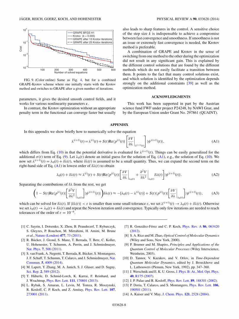
FIG. 9. (Color online) Same as Fig. 4, but for a combinedGRAPE-Krotov scheme where one initially starts with the Krotovmethod and switches to GRAPE after a given number of iterations.

parameters, it gives the desired smooth control fields, and itworks for various nonlinearity parameters κ .

In contrast, the Krotov optimization without an appropriatepenalty term in the functional can converge faster but usually

also leads to sharp features in the control. A sensitive choiceof the step size k is indispensable to achieve a compromisebetween fast convergence and smoothness. If smoothness is notan issue or extremely fast convergence is needed, the Krotovmethod is preferable.

A combination of GRAPE and Krotov in the sense ofswitching from one method to the other during the optimizationdid not result in any significant gain. This is explained bythe different control solutions that are found by the differentmethods which do not easily facilitate a transition betweenthem. It points to the fact that many control solutions exist,and which solution is identified by the optimization dependsstrongly on the additional constraints [39] as well as theoptimization method.

ACKNOWLEDGMENTS

This work has been supported in part by the Austrianscience fund FWF under project P24248, by NAWI Graz, andby the European Union under Grant No. 297861 (QUAINT).

APPENDIX

In this appendix we show briefly how to numerically solve the equation

λ(i+1)(t) = λ(i)(t) + S(t)Re〈p(i)(t)|[∂V

∂λ

∣∣∣∣λ(i+1)(t)

]|ψ (i+1)(t)〉, (A1)

which differs from Eq. (10) in that the potential derivative is evaluated for λ(i+1)(t). Things can be easily generalized for theadditional σ (t) term of Eq. (9). Let λ0(t) denote an initial guess for the solution of Eq. (A1), e.g., the solution of Eq. (10). Wenow set λ(i+1)(t) = λ0(t) + δλ(t), where δλ(t) is assumed to be a small quantity. Thus, we can expand the second term on theright-hand side of Eq. (A1) in lowest order of δλ(t) to obtain

λ0(t) + δλ(t) ≈ λ(i)(t) + S(t)Re〈p(i)(t)|[∂V

∂λ

∣∣∣∣λ0(t)

+ ∂2V

∂λ2

∣∣∣∣λ0(t)

δλ(t)

]|ψ (i+1)(t)〉. (A2)

Separating the contributions of δλ from the rest, we get(1 − S(t)Re〈p(i)(t)|

[∂2V

∂λ2

∣∣∣∣λ0(t)

]|ψ (i+1)(t)〉

)δλ(t) ≈ −[λ0(t) − λ(i)(t)] + S(t)〈p(i)(t)|

[∂V

∂λ

∣∣∣∣λ0(t)

]|ψ (i+1)(t)〉, (A3)

which can be solved for δλ(t). If |δλ(t)| < ε is smaller than some small tolerance ε, we set λ(i+1)(t) → λ0(t) + δλ(t). Otherwisewe set λ0(t) → λ0(t) + δλ(t) and repeat the Newton iteration until convergence. Typically only few iterations are needed to reachtolerances of the order of ε = 10−6.

[1] C. Sayrin, I. Dotsenko, X. Zhou, B. Peaudecerf, T. Rybarczyk,S. Gleyzes, P. Rouchon, M. Mirrahimi, H. Amini, M. Bruneet al., Nature (London) 477, 73 (2011).

[2] R. Bucker, J. Grond, S. Manz, T. Berrada, T. Betz, C. Koller,U. Hohenester, T. Schumm, A. Perrin, and J. Schmiedmayer,Nat. Phys. 7, 508 (2011).

[3] S. van Frank, A. Negretti, T. Berrada, R. Bucker, S. Montangero,J. F. Schaff, T. Schumm, T. Calarco, and J. Schmiedmayer, Nat.Commun. 5, 4009 (2014).

[4] M. Lapert, Y. Zhang, M. A. Janich, S. J. Glaser, and D. Sugny,Sci. Rep. 2, 589 (2012).

[5] T. Haberle, D. Schmid-Lorch, K. Karrai, F. Reinhard, andJ. Wrachtrup, Phys. Rev. Lett. 111, 170801 (2013).

[6] L. Rybak, S. Amaran, L. Levin, M. Tomza, R. Moszynski,R. Kosloff, C. P. Koch, and Z. Amitay, Phys. Rev. Lett. 107,273001 (2011).

[7] R. Gonzalez-Ferez and C. P. Koch, Phys. Rev. A 86, 063420(2012).

[8] S. A. Rice and M. Zhao, Optical Control of Molecular Dynamics(Wiley and Sons, New York, 2000).

[9] P. Brumer and M. Shapiro, Principles and Applications of theQuantum Control of Molecular Processes (Wiley Interscience,Weinheim, 2003).

[10] D. Tannor, V. Kazakov, and V. Orlov, in Time-DependentQuantum Molecular Dynamics, edited by J. Broeckhove andL. Lathouwers (Plenum, New York, 1992), pp. 347–360.

[11] J. Werschnik and E. K. U. Gross, J. Phys. B: At., Mol. Opt. Phys.40, R175 (2007).

[12] J. P. Palao and R. Kosloff, Phys. Rev. Lett. 89, 188301 (2002).[13] P. Doria, T. Calarco, and S. Montangero, Phys. Rev. Lett. 106,

190501 (2011).[14] A. Kaiser and V. May, J. Chem. Phys. 121, 2528 (2004).

033628-8

OPTIMAL QUANTUM CONTROL OF BOSE-EINSTEIN . . . PHYSICAL REVIEW A 90, 033628 (2014)

[15] T. Caneva, T. Calarco, and S. Montangero, Phys. Rev. A 84,022326 (2011).

[16] A. Konnov and V. Krotov, Autom. Remote Control (Engl.Transl.) 60, 1427 (1999).

[17] S. E. Sklarz and D. J. Tannor, Phys. Rev. A 66, 053619 (2002).[18] N. Khaneja, T. Reiss, C. Kehlet, T. Schulte-Herbruggen, and

S. J. Glaser, J. Magn. Reson. 172, 296 (2005).[19] S. Machnes, U. Sander, S. J. Glaser, P. de Fouquieres,

A. Gruslys, S. Schirmer, and T. Schulte-Herbruggen, Phys. Rev.A 84, 022305 (2011).

[20] R. Eitan, M. Mundt, and D. J. Tannor, Phys. Rev. A 83, 053426(2011).

[21] T. Caneva, M. Murphy, T. Calarco, R. Fazio, S. Montangero,V. Giovannetti, and G. E. Santoro, Phys. Rev. Lett. 103, 240501(2009).

[22] U. Hohenester, P. K. Rekdal, A. Borzi, and J. Schmiedmayer,Phys. Rev. A 75, 023602 (2007).

[23] U. Hohenester, Comput. Phys. Commun. 185, 194 (2014).[24] D. M. Reich, M. Ndong, and C. P. Koch, J. Chem. Phys. 136,

104103 (2012).[25] Y. Shin, M. Saba, T. A. Pasquini, W. Ketterle, D. E. Pritchard,

and A. E. Leanhardt, Phys. Rev. Lett. 92, 050405 (2004).[26] T. Schumm, S. Hofferberth, L. M. Andersson, S. Wildermuth,

S. Groth, I. Bar-Joseph, J. Schmiedmayer, and P. Kruger, Nat.Phys. 1, 57 (2005).

[27] J. Grond, U. Hohenester, I. Mazets, and J. Schmiedmayer, NewJ. Phys. 12, 065036 (2010).

[28] A. P. Peirce, M. A. Dahleh, and H. Rabitz, Phys. Rev. A 37,4950 (1988).

[29] R. Bucker, T. Berrada, S. van Frank, T. Schumm, J. F. Schaff,J. Schmiedmayer, G. Jager, J. Grond, and U. Hohenester,J. Phys. B: At., Mol. Opt. Phys. 46, 104012 (2013).

[30] A. Leggett, Rev. Mod. Phys. 73, 307 (2001).[31] J. Grond, G. von Winckel, J. Schmiedmayer, and U. Hohenester,

Phys. Rev. A 80, 053625 (2009).[32] G. Jager and U. Hohenester, Phys. Rev. A 88, 035601 (2013).[33] A. Borzi and U. Hohenester, SIAM J. Sci. Comput. 30, 441

(2008).[34] G. von Winckel and A. Borzi, Inverse Probl. 24, 034007

(2008).[35] C. M. Dion and E. Cances, Comput. Phys. Commun. 177, 787

(2007).[36] D. P. Bertsekas, Nonlinear Programming (Athena Scientific,

Cambridge,1999).[37] J. P. Palao and R. Kosloff, Phys. Rev. A 68, 062308 (2003).[38] I. Lesanovsky, T. Schumm, S. Hofferberth, L. M. Andersson,

P. Kruger, and J. Schmiedmayer, Phys. Rev. A 73, 033619(2006).

[39] J. P. Palao, D. M. Reich, and C. P. Koch, Phys. Rev. A 88, 053409(2013).

033628-9