Embed Size (px)
Citation preview

Astin Bulletin 41(2), 547-574. doi: 10.2143/AST.41.2.2136988 © 2011 by Astin Bulletin. All rights reserved.
OPTIMAL REINSURANCE REVISITED –POINT OF VIEW OF CEDENT AND REINSURER
BY
WERNER HÜRLIMANN
ABSTRACT
It is known that the partial stop-loss contract is an optimal reinsurance form under the VaR risk measure. Assuming that market premiums are set according to the expected value principle with varying loading factors, the optimal rein-surance parameters of this contract are obtained under three alternative single and joint party reinsurance criteria: (i) strong minimum of the total retained loss VaR measure; (ii) weak minimum of the total retained loss VaR measure and maximum of the reinsurer’s expected profi t; (iii) weak minimum of the total retained loss VaR measure and minimum of the total variance risk meas-ure. New conditions for fi nancing in the mean simultaneously the cedent’s and the reinsurer’s required VaR economic capital are revealed for situations of pure risk transfer (classical reinsurance) or risk and profi t transfer (design of internal reinsurance or reinsurance captive owned by the captive of a corporate fi rm).
KEYWORDS
Optimal reinsurance, reinsurance captive, risk and profi t transfer, partial stop-loss, economic capital, VaR, expected value principle, loading factor, mean fi nancing property
1. INTRODUCTION
Reinsurance is an important risk transfer instrument that leads to a more effective risk management through reduction of required economic capital. Optimal reinsurance is a widely discussed and complex actuarial topic that fi nds a great variety of different answers. There are two kinds of optimization problems:
P1) Find the optimal reinsurance form under given criteria for a given set of ceded and/or retained loss functions.
P2) For a given optimal reinsurance form, that is a solution to problem P1, determine the optimal reinsurance parameters (e.g. optimal retention, expected profi t, reinsurance price, etc.) under given criteria.
94838_Astin41-2_10_Hurlimann.indd 54794838_Astin41-2_10_Hurlimann.indd 547 2/12/11 08:332/12/11 08:33

548 W. HÜRLIMANN
Concerning problem P1 early results have shown that the stop-loss contract is an optimal reinsurance form under the variance risk measure by minimizing the variance of a portfolio’s retained loss for a fi xed reinsurance premium (e.g. Borch (1960), Kahn (1961), Arrow (1963/74), Ohlin (1969), etc.), which yield optimality under the cedent’s point of view. By minimizing the variance of a portfolio’s ceded loss for a fi xed reinsurance premium, Vajda (1962) has iden-tifi ed the quota-share contract as optimal reinsurance form, which yield opti-mality under the reinsurer’s point of view. Obviously, there is a confl ict of interests between the parties involved in a reinsurance program. As pointed out by Borch (1969) “an arrangement which is very attractive to one party may be quite unacceptable to the other”. Since publication of Borch’s seminal work (see Borch (1990) for collected papers), optimal solutions for both the cedent and the reinsurer have scarcely been discussed, although some papers devoted to joint optimality criteria have been published (e.g. Ignatov et al. (2004), Kaishev and Dimitrova (2006), Dimitrova and Kaishev (2010)).
In recent years various solutions to problem P1 and P2 under the value-at-risk measure (VaR) and the conditional value-at-risk measure (CVaR) have been obtained (e.g. Cai and Tan (2007), Cai et al. (2008), Bernard and Tian (2009), Cheung (2010), Chi and Tan (2010)). In the present paper, we show that within this framework it is possible to determine solutions that are opti-mal from the cedent’s and reinsurer’s point of views. Alternatively, we obtain optimal solutions under the total variance risk measure (sum of the ceded and retained variance of the loss) considered earlier by the author (in particular Hürlimann (1994a/b, 1996, 1999)).
The paper is organized as follows. Section 2 recalls the necessary and suf-fi cient conditions for the existence of the optimal reinsurance form under the VaR risk measure as fi rst identifi ed by Cai et al.(2008). The Sections 3 and 4 are devoted to the optimal design of the partial stop-loss contract with ceded loss function f(x) = a(x – d)+, a ! (0,1], d > 0, which is an optimal reinsurance form under the VaR risk measure. We assume throughout that the market premium and the reinsurance premium are set according to the expected value principle with varying loading factors. Proposition 3.1 determines the optimal reinsurance parameters by minimizing the VaR measure of the total retained loss for an arbitrary confi dence level (strong minimum). Proposition 3.2 pro-poses an alternative solution by minimizing the VaR measure of the total retained loss for a suffi ciently high confi dence level (weak minimum) and by maximizing the reinsurer’s expected profi t. A third optimal solution is found in Proposition 4.1 under a weak minimum of the total retained loss VaR measure and a minimum of the total variance risk measure. Interesting and useful conditions for fi nancing in the mean simultaneously the cedent’s and the reinsurer’s required economic capital are derived for situations of pure risk transfer (classical reinsurance) or risk and profi t transfer (design of internal reinsurance or reinsurance captive owned by the captive of a corporate fi rm). Section 5 illustrates the obtained results for a lognormal and a gamma approx-imate distribution of the loss. Section 6 summarizes and concludes.
94838_Astin41-2_10_Hurlimann.indd 54894838_Astin41-2_10_Hurlimann.indd 548 2/12/11 08:332/12/11 08:33

OPTIMAL REINSURANCE REVISITED 549
2. OPTIMAL REINSURANCE FORMS UNDER THE VAR RISK MEASURE
A reinsurance contract determines the rules according to which premium pay-ments and unearned premium reserves, as well as claim payments, case reserves and IBNR reserves are split between the ceding and the reinsurance compa-nies. In a simplifi ed approach let S be the (aggregate) loss of an insurance portfolio, which is supposed to be insured against a market premium P.We assume that S is a non-negative integrable random variable with cumula-tive distribution FS (x) = P(S # x), survival distribution FS (x) = 1 – FS (x), and positive mean m = E [S ] > 0. We assume that FS (x) is strictly increasing and continuous on (0, 3), with a possible jump at 0. The quantile function of S is defi ned and denoted by QS(u) = inf {x : FS (x) $ u}. The stop-loss transform of S is denoted by pS(x) = E [(S – x)+]. We use that pS(x) = FS (x) · mS(x), where mS(x) denotes the mean excess function. Let Sr, Sc be the loss random variables representing the reinsurer’s loss and the cedent’s loss in the presence of reinsurance such that S = Sc + Sr holds, and denote the expected values of these losses by mr = E [Sr], mc = E[Sc ]. We assume that the market premium and the reinsurance premium Pr are set according to the expected value principle such that
P = (1 + q) m, Pr = (1 + qr) mr, (2.1)
where q is the market loading factor without reinsurance, and qr is the loading factor of the reinsurer. Note that this assumption is in agreement with actu-arial practice, where usually either the reinsurance premium or the reinsurance loading factor is predetermined. Then, the cedent’s retained premium andthe corresponding (implicit) loading factor qc are determined by Pc = P – Pr = (1 + qc) mc. Given an insured loss (q, S) and the reinsurance loading factor qr, the actuarial problem of optimal reinsurance is to determine, under given criteria, the optimal reinsurance premium Pr = (1 + qr) mr, or equivalently, either the optimal retained premium Pc = P – Pr or the cedent’s loading factor qc = q – (qr – q) mr / (m – mr).
The VaR and CVaR of a random variable X at the confi dence level a ! (0,1) are defi ned as VaRa [X ] = QX(a) and CVaRa[X ] = E [X |X > VaRa[X ] ] respec-tively. Let f (x) be a real, increasing and convex function on (0, 3), which satis-fi es 0 # f (x) # x, called ceded loss function, such that Sr = f (S ) representsthe ceded loss. The set of all possible ceded loss functions is denoted as C.The reinsurance premium corresponding to f ! C is denoted by Pr
f(S) = (1 + qr) E [ f(S )]. The total retained loss, which is the sum of the cedent’s loss and the reinsurance premium, is denoted by Tc
f(S) = S – f (S ) + Prf(S). The
optimal reinsurance problems of type P1 studied by Cai et al. (2008) and Cheung (2010) are stated as follows:
c c c c ((S S S S( ( ) .min minaR T VaR T aR T aR Ta a a af C f C=
! !
f f*f *f) )V V=) , CVC8 8B B8 8B B
(2.2)
94838_Astin41-2_10_Hurlimann.indd 54994838_Astin41-2_10_Hurlimann.indd 549 2/12/11 08:332/12/11 08:33
550 W. HÜRLIMANN
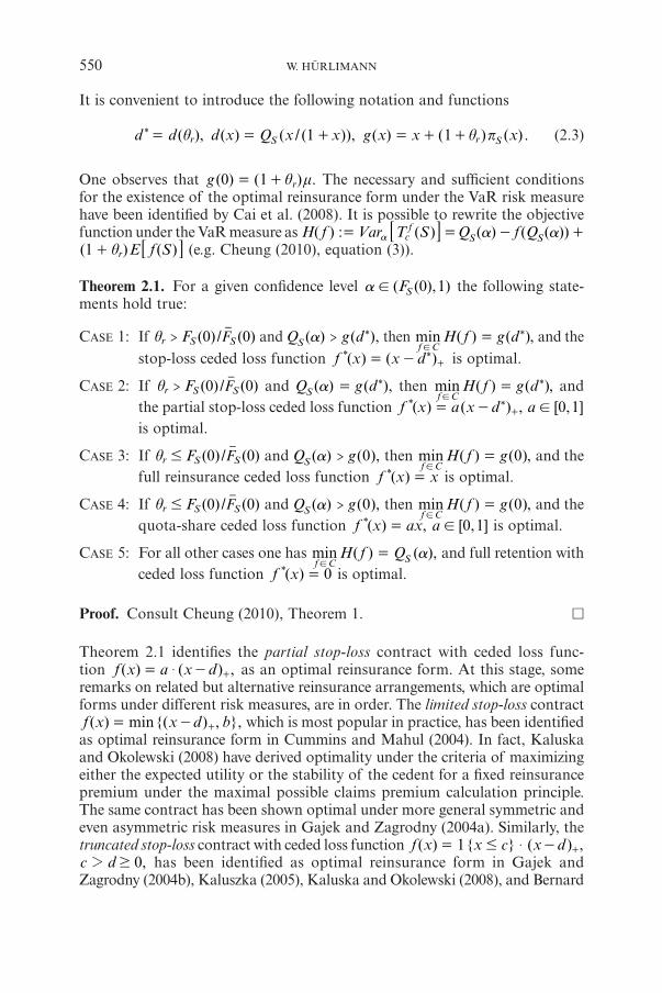
It is convenient to introduce the following notation and functions
x Sq= Sr r( ()( ), ( ( / (1 ), ) ( ) ) .d d d x Q g x x xp= + = + +q ) x 1* (2.3)
One observes that q( ) ( ) .g 0 r m= +1 The necessary and suffi cient conditions for the existence of the optimal reinsurance form under the VaR risk measure have been identifi ed by Cai et al. (2008). It is possible to rewrite the objective function under the VaR measure as c( a( )S S(Sa a) ( ( ))H Var T Q f Q= - +f )f := 8 B
r(1 ) ( )E f S+ q 7 A (e.g. Cheung (2010), equation (3)).
Theorem 2.1. For a given confi dence level Sa ( ( ), )0 1! F the following state-ments hold true:
CASE 1: If r (0) / (0)F> S Sq F and a( )S (> dQ g *), then ( (d) ,min g *=f C!
)H f and the stop-loss ceded loss function +d((f x x *= -) )* is optimal.
CASE 2: If r (0) / (0)F> S Sq F and a( )S (dQ g *= ), then ( (d) ,min g *=f C!
)H f and the partial stop-loss ceded loss function ,d( ( ) [ , ]f x a a 0 1* != - +) x* is optimal.
CASE 3: If r ( ) / ( )F 0 0S S#q F and a( )S (Q g 0> ), then ( () ,min g 0=f C!
)H f and the full reinsurance ceded loss function (f x x=)* is optimal.
CASE 4: If r ( ) / ( )F 0 0S S#q F and a( )S (Q g 0> ), then ( () ,min g 0=f C!
)H f and the quota-share ceded loss function ( , [ , ]f x ax a 0 1!=)* is optimal.
CASE 5: For all other cases one has S( a) ( ),min Q=f C!
H f and full retention with ceded loss function (f x 0=)* is optimal.
Proof. Consult Cheung (2010), Theorem 1. ¡
Theorem 2.1 identifi es the partial stop-loss contract with ceded loss func-tion ,d(f a= +x) -$ ( )x as an optimal reinsurance form. At this stage, some remarks on related but alternative reinsurance arrangements, which are optimal forms under different risk measures, are in order. The limited stop-loss contract
,d( {( ) },minf b= - +x) x which is most popular in practice, has been identifi ed as optimal reinsurance form in Cummins and Mahul (2004). In fact, Kaluska and Okolewski (2008) have derived optimality under the criteria of maximizing either the expected utility or the stability of the cedent for a fi xed reinsurance premium under the maximal possible claims premium calculation principle. The same contract has been shown optimal under more general symmetric and even asymmetric risk measures in Gajek and Zagrodny (2004a). Similarly, the truncated stop-loss contract with ceded loss function d-( { } ( ) ,f x c1 #= +x x) $
0,c d2 $ has been identifi ed as optimal reinsurance form in Gajek and Zagrodny (2004b), Kaluszka (2005), Kaluska and Okolewski (2008), and Bernard
94838_Astin41-2_10_Hurlimann.indd 55094838_Astin41-2_10_Hurlimann.indd 550 2/12/11 08:332/12/11 08:33
OPTIMAL REINSURANCE REVISITED 551
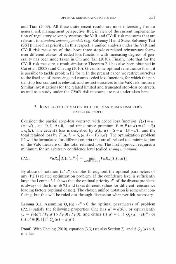
and Tian (2009). All these quite recent results are most interesting from a general risk management perspective. But, in view of the current implementa-tion of regulatory solvency systems, the VaR and CVaR risk measures that are relevant to standard solvency models (e.g. Solvency II and Swiss Solvency Test (SST)) have fi rst priority. In this respect, a unifi ed analysis under the VaR and CVaR risk measures of the above three stop-loss related reinsurance forms over different classes of ceded loss functions with increasing degrees of gen-erality has been undertaken in Chi and Tan (2010). Finally, note that for the CVaR risk measure, a result similar to Theorem 2.1 has also been obtained in Cai et al. (2008) and Cheung (2010). Given some optimal reinsurance form, it is possible to tackle problem P2 for it. In the present paper, we restrict ourselves to the fi xed set of increasing and convex ceded loss functions, for which the par-tial stop-loss contract is relevant, and restrict ourselves to the VaR risk measure. Similar investigations for the related limited and truncated stop-loss contracts, as well as a study under the CVaR risk measure, are not undertaken here.
3. JOINT PARTY OPTIMALITY WITH THE MAXIMUM REINSURER’SEXPECTED PROFIT
Consider the partial stop-loss contract with ceded loss function (f a=x) $d( ) , [0,1], 0,a d >!- +x and reinsurance premium r r rq( , ) ( )P P a d= = +1
( .a dSp ) The cedent’s loss is described by d( , ( )S a d S a Sc $- - +=) and the total retained loss by c rc( , ) ( , ) ( , ) .T a d S a d P a d= + The optimization problem P2 will be formulated for different criteria that are all related to a minimization of the VaR measure of the total retained loss. The fi rst approach requires a minimum for an arbitrary confi dence level (called strong minimum)
(P2.1) ,c cd ( , )a d( ) minVaR T a VaR Ta a* *
[ , ]a d0 1 0>! ,=8 7B A
By abuse of notation , d( )a* * denotes throughout the optimal parameters of any (P2.1) related optimization problem. If the confi dence level is suffi ciently large the Lemma 3.1 shows that the optimal priority d* of the diverse problems is always of the form r( )d q and takes different values for different reinsurance loading factors (optimal or not). The chosen unifi ed notation is somewhat con-fusing, but this will be ruled out through discussion whenever felt necessary.
Lemma 3.1. Assuming S da( )Q 0> >* the optimal parameters of problem (P2.1) satisfy the following properties. One has rd ( )d* = q , or equivalently
r (d d() / ) (0) / (0),F F>* *S S S S=q FF and either (i) a 1* = if S (da( )Q g> *) or
(ii) ! [ , ]a 0 1* if S (da( ) .Q g *= )
Proof. With Cheung (2010), equation (3.3) (see also Section 2), and if S da( ) ,Q > one has
94838_Astin41-2_10_Hurlimann.indd 55194838_Astin41-2_10_Hurlimann.indd 551 2/12/11 08:332/12/11 08:33

552 W. HÜRLIMANN
S S
S
c ( (
(
r
r
a a
a
, ,a a q
q
(( ) ) ) ) )
( ) ( ) ) .
(
(1 )
h d VaR T d Q a Q d a
a d d Qa
a S
S
$
$ $
= - -
= + +
= + +
+ -
( )
1
1 d
p
p7 7
7
A A
A
The minimum depends upon the partial derivatives (use that ( )x = ( )xdxd
S S-p F )
S (r raq q( ) ( ) ), 1 ( ) ( ) .h d d Q h a da S d S$= + + - = - +1 1 Fp " ,
The necessary fi rst order condition h 0d = implies that r (d1 1 / ),*S+ =q F or
equivalently ( (r F d d) / ) .* *S S=q F By defi nition of the function d (x) in (2.3) this
is equivalent to rd = .(d* q ) Now, for rd d ( ),d *= = q one has by defi nition of (x)g in (2.3) that
( S S( (a a(d d= da ) ) ),h m Q g Q* * *S+ - = -)
and similarly S (a a, (a d d( ) ( ) ) .h a g Q* *$ $= + -) 1
If h 0<a then ,a d( )h * is strictly decreasing, hence ,a 1* = and if ah 0= any ! [ ]a 1* ,0 is optimal. In both cases one has , ,c (d d d( ) ( )VaR T a h a ga
* * * * *= = )8 B as in Theorem 2.1. ¡
Similarly to the above, the optimal cedent’s loading factor is denoted by c .q* The next result describes the complete solution of problem P2 with respect to criterion (P2.1). The obtained result is a reformulation of the Cases 1 and 2 of Theorem 2.1.
Proposition 3.1. Given an insured loss ( ),Sq and a reinsurance loadingfactor satisfying r(0) / (0) ,F <S S !q qF assume that c0 ,# # qq* as well as
S (a m) / ( ) .Q 0> SF Then, the optimal ceded partial stop-loss function (f x =)*
d d!( ) , [0,1] ,a a 0>* * * *- + ,$ x under criterion (P2.1) is completely described by the following conditions. The optimal priority is given by rd ( )d* != q
max( , ]d0 ,* where maxd * is the unique solution of the implicit equation
(C1.1) S (amax max( ) ) .d m d QS+ =* *
The loading factors are necessarily given by and must satisfy the inequalities
(C1.2)
( )( )
( )( )
( )( )
dd
dd
dd
c
c
( )
( )
rr
r rr
( )
( )
dd
d
d
d
pmax
max
maxmax
,
, , ,max
Fd
aa
Fd
0 0 < <<
<
*
*
*
**
* *
* *
*
**
S
S
S
S
S
S
S
S
S
S
# #
#
qm
mm
qmm
=-
=
-=
-= =
*
*
q qq q
q q q qq q#
p
pp
pp
-
- -
m,
d0
F
F
*
*
*** 4
94838_Astin41-2_10_Hurlimann.indd 55294838_Astin41-2_10_Hurlimann.indd 552 2/12/11 08:332/12/11 08:33

OPTIMAL REINSURANCE REVISITED 553
and the optimal partial stop-loss factor ! [ , ]a 0 1* is determined as follows:
(C1.3)
c
c=
r
d
d
max
maxmax
,
( )[0,1], .
a
d
dd
1 0 < <
*
*
*
S
$ !
qq q m
-
-=
q *
*
,*
**
p
Z
[
\
]]
]]
Proof. By Lemma 3.1 and its proof one has = rd ( )d* q and +( (d dd ) .g m* * *S=)
One has (! 0,dd max]* * because (g x) is strictly increasing. Since the function
S(a(x) )h S= (x m x Q+ ) - is strictly increasing on S(a( ))0,Q with (aS )( )h 0>Q and S (a( ) (0) ( ) )0 0h Q 0<S S$ $m= -F F by assumption, the solution to (C1.1) is unique. On the other hand, the decomposition r cP P P= + is equivalent to the equality (here for the optimal solution)
c c= r (( ) ( ) ) .d* *Sq m q- -q * *q pa (3.1)
Assume for the moment that c r,<#q q* q which will be shown below. If d max0 d< <* * one must have 1* =a by the Case 1 of Theorem 2.1, which shows
the fi rst formula in (C1.3). The fi rst formula in (C1.2) follows from (3.1). If d maxd* = * the second formula in (C1.3) follows also from (3.1). Since 1*#a the equation (3.1) implies the inequality cr ( () ( )),d d* *
S S# q mm- -q q * pp which implies the fi rst inequality for cq* in the second formula in (C1.2). Moreover, using the assumption c ,#q q* one obtains from the same inequality that r#q q and more stringently r<q q by the assumption r ,! qq hence c r<#q q q* . ¡
Remarks 3.1.
(i) The condition c r<#q q q* means that the reinsurer covers stop-loss rein-surance at a higher loading factor than the cedent. In fact, if cq q=* either the optimal priority is the unique solution (! 0,dd max)* * of r ( )d*
Sqm = q p (if it exists) or one must have 0* =a (no reinsurance) in case d maxd* = * . Excluding the fi rst situation as a singular exception, reinsurance occurs only if the strict inequality c r<<q q q* holds. In fact, the inequality c r<q q* has been derived in the Appendix of Hürlimann (2010) by means of “ordering of risks” considerations. The assumption r ! qq is not restric-tive. Indeed, if cr !q q=q * the equality (3.1) is only possible for the choice
1, 0* *= =da of full reinsurance (excluded by assumption), and the remaining possibility cr q q= =q * contradicts the inequality c r<q q* .
(ii) The pure stop-loss case 1* =a is somewhat ambiguous. While the cedent’s loading factor is uniquely determined as a function of the optimal priority through S ( r rd q( ))Q* = +q 1/ , the reinsurance loading factor varies in the range r max max( (0) / (0), ( )/ ( )]F F d dS S S S!q F F* * . However, this fact may beof practical value, because the reinsurance loading factor can usually be
94838_Astin41-2_10_Hurlimann.indd 55394838_Astin41-2_10_Hurlimann.indd 553 2/12/11 08:332/12/11 08:33

554 W. HÜRLIMANN
chosen by the reinsurer (see also the comment (i) of the Remarks 3.2). Extending the optimality criterion taking into account the reinsurer’s point of view will resolve this ambiguity and yield well-defi ned optimal reinsur-ance loading factors that are denoted rq* (by abuse of notation).
A drawback of the obtained optimal design is the fact that it only provides optimality from the cedent’s point of view. To overcome this possibly unre-alistic limitation we consider alternative optimization criteria, which takeinto account both the cedent’s and reinsurer’s point of views. Our considera-tions will include a solvency perspective. We take into account the required VaR economic capitals of both parties and compare them to their under-writing expected profi ts. The retained VaR economic capital for a given con-fi dence level a depends only upon the centered retained loss and it is defi ned by mc= -a [ [ ]EC VaRac c
VaR ]S S: . One has the relationship
c cra [ [ [ ,EC VaR P VaR EGa ac c rm m= - = -VaR ]S T T- -] ] (3.2)
where
rrr( , )EG EG a d Pr r Sm= = - = q ( )dap (3.3)
denotes the reinsurer’s expected profi t. Since the VaR measure is additive for comonotonic random variables, and ,Sc rS are comonotonic, the ceded VaR economic capital at the confi dence level a is defi ned and determined by
m c=a a a[ [ ] [ ] [EC VaR EC ECS a rr r - = SVaR VaR VaRS -] ]S: , (3.4)
where ma [ [ ]EC VaRS a= -VaR S] represents the VaR economic capital without reinsurance. For later use we introduce also the retained expected profi t defi ned and denoted by
c -( , ) ( ( )) .EG EG a d P a dc c c c Sm m= = -= q p (3.5)
Before proceeding with alternatives let us mention the following interesting and useful properties. We use the notations , ,cd dr cr( ), ( ),S S S S* * * *= =a a* *
, ,d dr c( ), ( )EG EG EG EG* * * *r c= =a a** .
Corollary 3.1. Under the assumptions of Proposition 3.1 the reinsurer’s expected profi t of the optimal design, as a function of the ceded VaR economic capital, is given by
S (a(a r ) ) .EG EC S m d Q* *S= + -VaR
r d* +* 8 B (3.6)
94838_Astin41-2_10_Hurlimann.indd 55494838_Astin41-2_10_Hurlimann.indd 554 2/12/11 08:332/12/11 08:33

OPTIMAL REINSURANCE REVISITED 555
Moreover, in the special case S (a)P Q= (percentile premium calculation principle), the retained expected profi t, as a function of the retained VaR economic capital, is given by
c S (a d (ac ) .EG EC S * *S= - - mVaR Q d** )+8 B (3.7)
Proof. By the proof of Lemma 3.1, one has for the optimal design cTVaRa =*8 B
(d )g * . Substituting this and (3.2) into (3.4) one gets
c S (T a (da ar r r[ ] ) ) .EC S EC VaR EG Q g EGa*m- + = - +VaR VaR S= + * ** *8 8B B
Since ( (d d d) )g m* * *S= + one obtains (3.6). In the special case one has
S S S( ( (
c
a a a( (d d
Sa a a
c
r
r
[ ]
) ) ) ) ),
EC EC EC S
Q EG g Q EG g Q* *m
-
= - - + - = + -
VaR VaR VaRS=
*
*
*
*8 8B B
where the last equality follows from the relationship S (a)Q Pm m- = - =
c rEG EG+* *. ¡
The interpretation of Corollary 3.1 is quite instructive from an economic point of view. For this purpose we need a concept that describes the fact that a given deterministic quantity is fi nanced in the mean by another stochastic quantity.
Defi nition 3.1. A deterministic liability L is weakly (strongly) mean fi nanced by a stochastic profi t G if the mean inequality G $[ ]E L (mean equality
LG[ ]E = ) holds.
In the Case 2 of Theorem 2.1, i.e. d maxd* = * , Corollary 3.1 simplifi es by equa-tion (C1.1) to the relationships a rrEG EC SVaR=* *8 B and cacEG EC SVaR=* *8 B. From an economic management perspective the fi rst one means that the reinsurer’s required VaR economic capital is strongly mean fi nanced by the reinsurer’s profi t
rG P Sr r= - . Even more, in the mentioned special case, the cedent’s required VaR economic capital is also strongly mean fi nanced, namely by the cedent’s profi t c cG P Sc = - . In practice, these situations might be unrealistic. First, the special case implies that the market premium S (a)P Q= , which is set according to the percentile premium calculation principle, might not be competitive. Second, a reinsurer’s might not enter into such a zero-sum profi t strategy and opt for higher expected profi t at the cost of higher required economic capital.
Fortunately, the relationship (3.2) suggests at least two further optimization problems. First, one sees that minimizing c[VaRa T ] and maximizing EGr ren-ders actually ca [EC SVaR ] minimum. This can be formulated as single party optimization problem (point of view of cedent):
94838_Astin41-2_10_Hurlimann.indd 55594838_Astin41-2_10_Hurlimann.indd 555 2/12/11 08:332/12/11 08:33

556 W. HÜRLIMANN
(P2.1’) , d ca a( ) ( ,minEC S EC S a* *[ , ],a dc 0 1 0! $
VaR VaRa )d=8 7B A
The optimal solution of this problem coincides with full reinsurance.
Corollary 3.2. Assume S (a)Q > m. Given an insured loss ( , )q S and the reinsur-ance loading factor rq , the optimal ceded partial stop-loss function (f x * $=) a*
$d d( ) , [0,1], 0* * *!- +x a , under criterion (P2.1’) is full reinsurance, i.e. 1, =d= 0* *a .
Proof. With Cheung (2010), equation (3.3), (see also Section 2), and (3.3), rewrite (3.2) as
d
d
S S
S S
( (
( (
c c ra a
a a
qa [ [ ) ( ) ) ( ) ( )
) ( ) ) ( ) .
EC S VaR EG Q a d
EG Q a d
a r S
r S
m
m m
- - - + +
- - = - - + -
+
+
VaR T Q
Q
1 a
a
=] ] -= p
p
Since this expression does not contain the variable rq , one sees that problem (P2.1’) is formally identical to the minimization problem cVaR m{ ( , )] }[min T a da[ , ],a d0 1 0
-! $
for a vanishing reinsurance loading factor r 0=q . Since S (a) ( )Q g 0> m= , the result follows from Case 3 of Theorem 2.1. ¡
A second meaningful two party optimization problem (point of view of cedent and reinsurer) is to minimize for a suffi ciently high confi dence level the VaR measure of the total retained loss and maximize the reinsurer’s expected profi t:
(P2.2) ,c d( ) ( , )minVaR T EG a da* *
( , ],a d r0 1 0>!
a =8 B for a suffi ciently high confi dence level a ,
, d( ) ( , )maxEG EG a d* *, ],(r
a dr0 1 0>
=!
a
To distinguish it from the strong minimum required by criterion (P2.1) the less stringent minimum in (P2.2) is called weak minimum. The slightly restricted optimization problem with a fi xed partial stop-loss factor ( , ]a 0 1! is consid-ered in Proposition 3.2 while Corollary 3.3 handles the unrestricted problem. As already stated in the comment (ii) of the Remarks 3.1 the obtained optimal reinsurance loading factors are denoted rq*.
Proposition 3.2. Given an insured loss ( , )Sq , assume that c r0 , !# #q q q q* * , and S (a d)Q 0> >* . Assume that the density function (x( ) 0f x >S S�) = F and its derivative (x)fS� exist for all x 0> . Then, the optimal ceded partial stop-loss function d d( ( ) ,f x a 0>* *$= - +) x , for fi xed ( , ]a 0 1! , under criterion (P2.2) is completely described as follows. A local maximum for the reinsurer’s
94838_Astin41-2_10_Hurlimann.indd 55694838_Astin41-2_10_Hurlimann.indd 556 2/12/11 08:332/12/11 08:33

OPTIMAL REINSURANCE REVISITED 557
expected profi t exists at the optimal priority = rd ( )d 0>* q* , if and only if the implicit equation
(C2.1) ( ( ( (d d d d) ) ) )f m F* * * *S S S S$ $= F
has a solution and one has
(C2.2) (( ( (d d d) ( 3 )) ) ) ( ) .f F df d 0>* * *S S S S S$ $ $ $- - �2 F p
The optimal reinsurance loading factor is necessarily given by
(C2.3) r((
((
dd
))
))
.F F
00
>*
*
S
S
S
Sq =*
F F
The optimal cedent’s loading factor is determined by and satisfi es the inequality
(C2.4) (
(d
dc
rr
))
aa
0 .*
*
S
S 1# #qm q
q q=-
-
ppq*
**
m
Proof. The necessary condition (C2.3) of optimality, that is r ( )d( ) / ,F dS S=q F has been shown in Lemma 3.1. It follows that r( , ) ( )EG a d dr S= =q ap
( ) ( )a F d m dS S$ $ . For ease of notation, set .( )d( ) ( ) ( ) ( )h d f d d F dS S S S2
$ $= -p F
Since (S )( ( )m x x xS S=) /p F , a calculation shows that 2( )d( , ) ( )
.dEG a d
ah dr
S2
2= $
F
A necessary condition for the existence of a local maximum is herewith (C2.1).
Further, using that (d )h 0* = at the optimal priority, one obtains EGd
r
d d
22
2=
=2
*
(d )
2(�
.ad
h*
*
S )$
F A second order suffi cient condition for a local maximum is here-
with ( ( ( (d d d d) ( ) ) )f= (d-) (2 3 ) )h d 0<* * * * *S S S S S-� p�f F$ $ $ F , which yields
condition (C2.2). The expression for the cedent’s loading factor in (C2.4) fol-lows from the equality (3.1) and the inequalities for the loading factors are shown as in the proof of Proposition 3.1. ¡
For a variable partial stop-loss factor ( , ]a 0 1! the optimal design is deter-mined as follows.
Corollary 3.3. Under the assumptions of Proposition 3.2 and variable stop-loss factor ( , ]a 0 1! the optimal design under criterion (P2.2) has a ceded stop-loss function df ( ( ) , 0x >* *= - + d) x , and is determined as follows. If it exists, the optimal priority rd = ( 0d >* q )* is solution of the implicit equation (C2.1) and (C2.2) must hold. Moreover, the optimal reinsurance loading factor is given by (C2.3) and the remaining loading factors satisfy the conditions
94838_Astin41-2_10_Hurlimann.indd 55794838_Astin41-2_10_Hurlimann.indd 557 2/12/11 08:332/12/11 08:33

558 W. HÜRLIMANN
(C2.4’) c(
rr(
( ((d
dd
dd
S
))),
))
.F
<*
*
*
*
*S S
S
S#m q q q
mqm q
=-
-=
p * **
pp
F
Proof. By the proof of Lemma 3.1 one has a(d d[ ( , ] ) ( )VaR a a g 1a* *
c $ $= + -T
S (a) .Q This is minimum, and d ( (F d d( ) ) )EG a m* * *r S S$ $=,a is maximum,
exactly when a 1= . The conditions (C2.4’) follow from (C2.4) through rear-rangement by setting a 1= . ¡
Remarks 3.2.
(i) In Proposition 3.2 and Corollary 3.3 the optimal reinsurance loading fac-tor is by (C2.3) a predetermined function of the optimal priority. If d* is very large, then rq* will be very large, which will be unrealistic in practice. In contrast to this, in Proposition 3.1 the reinsurance loading factor can be fi xed by the reinsurer, which is in agreement with practice. But then, unless (aS(d ) )g * = Q with d maxd* = * , one has (aS(d ) )g <* Q and only the pure stop-loss contract can be optimal by the Case 1 of Theorem 2.1. Based on reinsurance market data, it might be interesting to analyze whether Proposition 3.2 and Corollary 3.3 can generate unrealistic practical situations. As alternatives, it is still possible to consider similar optimization problems for the (optimal) limited and truncated stop-loss contracts men-tioned at the end of Section 2.
(ii) Corollary 3.3 proposes a method to identify the unknown optimal priority in Case 1 of Theorem 2.1. The optimal priority in (C2.1) can be reinterpreted as fi xed point of the quantile function
( SS
SS S( (
((
d d ddd
1) ))))
hhh* * *
*
*
S$= =00
Q Qm ,f p (3.8)
where
S S((S
SS
S( )x( )))
{ }, ( ) ( )( )
{ ( )},ln lnh xx
f xh x x
xxdx
d
Sdxd
S1
= = = =0
p p- -FF
F (3.9)
denote respectively the hazard rate function (also called failure rate, degree zero stop-loss rate), and the degree one stop-loss rate, (see Hürlimann (2000), Section 2).
(iii) Existence and uniqueness of the local maximum defi ned by (C2.1)-(C2.2) remain to be discussed. The numerical optimal priorities obtained in Sec-tion 5 are all uniquely determined. In general, it is felt that the fi xed point equation (3.8) might be helpful for resolving the open existence question using appropriate conditions for such equations. Uniqueness depends upon the number of sign changes of the function ( )h d in the proof of Proposition 3.2. Both questions have so far not been analyzed and go beyond the scope of the present investigation.
94838_Astin41-2_10_Hurlimann.indd 55894838_Astin41-2_10_Hurlimann.indd 558 2/12/11 08:332/12/11 08:33

OPTIMAL REINSURANCE REVISITED 559
4. JOINT PARTY OPTIMALITY WITH THE MINIMUM OF THE TOTAL
VARIANCE RISK MEASURE
From now on we will assume that the loss S has a fi nite variance [Var SS ]s =2 and we defi ne and denote the stop-loss transform of degree two by (x),S2p =
E +2( )x-S7 A. The stop-loss transform variance is defi ned and denoted by
S .2( ) ( ) ( )x x x,S S2s p= -2 pInstead of maximizing the reinsurer’s expected profi t besides minimizing in
a weak sense the total retained loss VaR, one might consider stabilization of the total variance of the retained and ceded loss. It is generally recognized that an appropriate reinsurance program should minimize unexpected fl uctuations and produce value through more stable insurance results (e.g. Venter (2001)). Suppose unexpected fl uctuations are measured using the variance, and thatthe unexpected total fl uctuations associated to the splitting of a risk in several components is measured using the total variance risk measure defi ned by the sum of the component variances. In the reinsurance situation this risk measure is defi ned and denoted by
S, ,S Sc c c$R S ar S ar S Cov S2S r r rs= -2V V+=6 6 6 6@ @ @ @ (4.1)
An alternative to (P2.2) is therefore the following optimization criterion (weak minimum of the cedent’s VaR measure of the total retained loss and minimum of the total variance risk measure):
(P2.3) , ( ,dc c a( ) )minVaR T VaR T da a* *
( , ]a d0 1 0>!
a,
=7 6A @ for all suffi ciently high con-fi dence levels a ,
, , ( , ( ,d d a a( ), ( ) ), )minR S S R S d S d* * * *( , ]S r a d S c rc 0 1 0>!
a a,
=7 6A @
We consider optimization under the restricted criterion (P2.3) for a fi xed par-tial stop-loss factor ( , ]a 0 1! . The “conjugate” or dual stop-loss transform defi ned by ((p ) )x x xS Sm= - + p and the dual mean excess function ( )xSm defi ned by ((p m) ( ) )Fx x xS S $= S are used.
Proposition 4.1. Given an insured loss ( ),Sq with fi nite variance Ss2 , assume
that c r0 , !# #q q q q* * , and (aS d) 0> >*Q . Assume that the density function ( )x( 0f x >S S) �= F exists for all x 0> . Then, the optimal ceded partial stop-
loss function d df ( ( ) ,x a 0>* *$= - +) x , for fi xed ( , ]a 0 1! , under criterion (P2.3) is completely described as follows. A local minimum for the total vari-ance of the retained and ceded loss exists at the optimal priority (d qrd = ) 0>* ,*
if and only if, ( , ]a 121
! , the implicit equation
(C3.1) ( (d d( 1) ) ) ,m 0* *S$ - =2 Sma - ,
has a solution and one has
94838_Astin41-2_10_Hurlimann.indd 55994838_Astin41-2_10_Hurlimann.indd 559 2/12/11 08:332/12/11 08:33

560 W. HÜRLIMANN
(C3.2) ( ( ( (d d d dS2 ) ) ) 2 ) .F f a 0>* * * * *S S S$ $ $ $m- - +a d pF ^ h
The optimal reinsurance loading factor is necessarily given by
(C3.3) r((dd
S S))
( )( )
.F F
00
>*
*S Sq =*
F F
The optimal cedent’s loading factor is determined by and satisfi es the inequality
(C3.4) c(
(rr
dd
0)
).<
*
*
S
S# #q
mqm q
q q=-
-
aa*
**
pp
Proof. The necessary condition (C3.3) has been shown in Lemma 3.1. According to (4.1) the total variance risk measure is minimal exactly when the covariance between the retained and ceded loss is maximum. To obtain an expression for this quantity, use that = ( ) , ( )S S a d a dc r$ $- - = -+ +S S S to get
,S Cov Varc $S , ( ) ( )
( ) ( ) .
Cov S d a d
a E d a d
a
,
r
S S S2
$
$ $ p
= - - -
= - - +
+ +
+ ( ) ( )
S S
S d dS am-2p p
8 7 7
7
B A A
A
$
$
.
.
But, one has ( )dd+( ) ( ) ( ) ( )E d d d dE d, SS2$ $ p- - + -= = ++ +S S S2 pS6 @ 7 A . Inserted in the preceding curly bracket one obtains
c, ( ) ( ) ( ( )) ( ) ( )
( ),
Cov S S a a d d d d a
a h d
1 1,r S S S S2$ $ $
$
p m= - + - + - -
=
( )dp p 2p8 B % /
with S=( )d a (p( ) ( ) ( ) )h d d dS S$ $s- +21 p . A necessary condition for a local maximum is (d =)h 0*� . Using that = = =S�� �S (p( ), ) ( ), ( )d d F d dS S S s- 2( )d Fp
2 ( ) ( )F d dS S- p one obtains
a2 ( )
1
- S
S
p( ) ( ) ( ) ( ) ( ) ( ) ( )
( ) ( ) (2 ) ( ) ( )
h d a F d d d d F d d
a F d d m d d
S S S S S
S S
$
$ $
= - - +
= - - Sm
� 1
,a
p pF
F
#
#
-
-
which implies the condition (C3.1). One notes that the condition ( , ]a 121
! is necessary for a local minimum. Indeed, if a 2
1# then ( )d = 0�h can only be
fulfi lled if (Sp )d 0# . Since (Sp )d is strictly increasing and (p ) 00S = onehas (Sp )d 0< for all d 0> and thus ( )d = 0�h is impossible for a 2
1# .
A second order suffi cient condition for a local maximum is (d ) 0h <*� . Since 1)( S ( )d d) {( ( ) ( ) ( )}a F d d dS S S$= -2 p- p�h a F one gets further
94838_Astin41-2_10_Hurlimann.indd 56094838_Astin41-2_10_Hurlimann.indd 560 2/12/11 08:332/12/11 08:33
OPTIMAL REINSURANCE REVISITED 561
1)(-
1) 2a
S S
S
p
p
( ) (2 ( ) ( ) ( ) ( )) ( ) ( ) ( ) ( )
( ) ( ( ) ( )) ( ) ( )
d a a d d F d d f d d F d d
a f d d d F d d
S S S S S S
S S S S
$
$
= - + -
= + -(2 ,
f p
p-a
F F
F
h� #
#
-
-
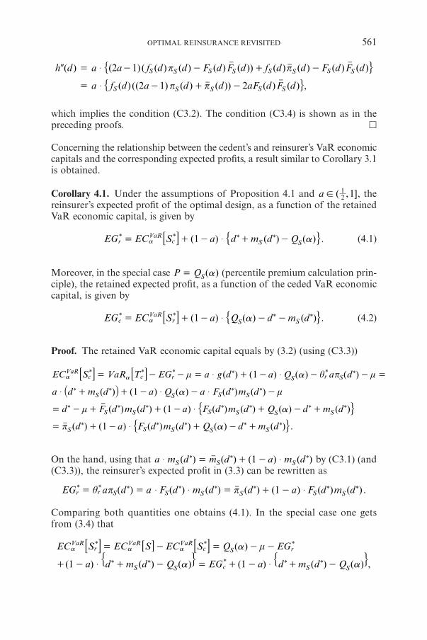
which implies the condition (C3.2). The condition (C3.4) is shown as in the preceding proofs. ¡
Concerning the relationship between the cedent’s and reinsurer’s VaR economic capitals and the corresponding expected profi ts, a result similar to Corollary 3.1 is obtained.
Corollary 4.1. Under the assumptions of Proposition 4.1 and ( , ]a 121
! , the reinsurer’s expected profi t of the optimal design, as a function of the retained VaR economic capital, is given by
(ac S )aSar ) ( .EG EC m d Q* *S$- + -VaR )= * ( d+ 1* 8 B # - (4.1)
Moreover, in the special case (aS )P = Q (percentile premium calculation prin-ciple), the retained expected profi t, as a function of the ceded VaR economic capital, is given by
(aSa drSac ) ) ( .EG EC m d* *S$- - -VaR )Q= * (+ 1* 8 B # - (4.2)
Proof. The retained VaR economic capital equals by (3.2) (using (C3.3))
(
(
(
(
c c a
a
a
a
(S
S
S
S
ra
a
a
a
(
( ( (
( ( ( ( (
( ( ( (
d d
d d d d
d d d d d d d
d d d d d
S
S Ta r
p
) ( ) ) )
) ( ) ) ) )
) ) ( ) ) ) ) )
) ( ) ) ) ) ) .
EC VaR EG a g
a m a F m
m F m m
F m m
a* *
* * * *
* * * * * * *
* * * * *
S
S S S
S S S S
S S S S
$ $
$ $ $
$
$
m q m
m
m
= - - = + - - - =
+ + - - -
= - + + - + - +
= + - + - +
aVaR Q
Q
Q
Q
1
1
1
1
* * **
F
p
_ i
8 8B B
#
#
-
-
On the hand, using that ( ( (d d a d) ) (1 ) )a m m* * *S S$ $= + -Sm by (C3.1) (and
(C3.3)), the reinsurer’s expected profi t in (3.3) can be rewritten as
(r ( ( ( ( (d d d d d dr p) ) ) ) (1 ) ) .EG a F m a F m* * * * * *S S S S S S$q= = = + -a* )$* $p
Comparing both quantities one obtains (4.1). In the special case one gets from (3.4) that
(
( (
c a
a a
S
S S
r
((d d dm
a a a r
c
)
( ) ) ) ( ) ) ) ,
EC S EC S EC S EG
a m EG a1 1* * * *S S$ $
m= - -
+ - + - = - + -
VaR VaR VaR Q
Q d Q
-* * =
+
*
*
8 7 8B A B
$ $. .
94838_Astin41-2_10_Hurlimann.indd 56194838_Astin41-2_10_Hurlimann.indd 561 2/12/11 08:332/12/11 08:33

562 W. HÜRLIMANN
where the last equality follows from the relationship (aS ) Pm m- = - =Qc rEG EG+* *. ¡
Remarks 4.1.
(i) The conditions (C3.1) and (C3.2) for the pure stop-loss contract a 1= have been further discussed and analyzed in Hürlimann (1999). The results in Corollary 4.1 are new. They provide an alternative to Corollary 3.3for identifying the unknown optimal priority in Case 1 of Theorem 2.1 (see point (iii) of the Remarks 3.2). Moreover, they suggest further appli-cation in risk management:
(ii) Consider “internal reinsurance” in a (re)insurance company or a “reinsur-ance captive” owned by a corporate business fi rm that acts as insurer either directly or via another direct insurance captive. The property
ca rEC EGS =VaR * *7 A means that the cedent’s required VaR economic capital is strongly mean fi nanced by the reinsurer’s profi t. What does this mean in practice? Let split the insurance loss of a fi rm between a direct insurance captive (acting as cedent) and a reinsurance captive in this optimal way. Since a reinsurance captive does not need to generate profi t from their reinsurance business, its profi t can be transferred to the direct insurance captive that covers herewith in the mean its required VaR economic cap-ital. As a consequence only the VaR economic capital of the reinsurance captive must be reserved by the fi rm. Though the reinsurer’s requiredVaR economic capital, given by ( (Sr a dp )EC S *
Sm- -a )VaR * Q=7 A , may be quite important, it is clearly less than the required VaR economic capital
(aSa [ ] )EC S m= -VaR Q for the original loss faced without a reinsurance arrangement. Though this implies a release of required VaR economic capital this is not a surprise per se because the premium for the original loss will include and fi nance in the mean the reinsurer’s profi t. Therefore, from an economic point of view the release of economical capital is just transferred to the original premium without a priori any economic benefi t.
(iii) In continuation of the discussion in (ii), in the special case of Corollary 4.1, the reinsurer’s VaR economic capital also coincides with the retained expected profi t. In this situation an overall strongly mean fi nancing strategy for an internal reinsurance or for a two party captive structure (direct insur-ance captive and reinsurance captive) can be designed by exchanging the profi ts between cedent and reinsurer. Setting the market premium equal to the percentile premium (aS )P = Q fulfi lls automatically the VaR eco-nomic capital requirements of both the cedent and the reinsurer. In this optimal way, the required VaR economic capital of a fi rm is not only mean fi nanced but also mean self-fi nanced by the cedent’s and reinsurer’s profi ts. Again, this is not a surprise because the VaR economic capital of the original loss is already strongly mean fi nanced by the original profi t in virtue of the equality (aSG S a[ ] ) [ ]E E EC Sm= = - =] VaRQ[ -P , and a splitting of the original loss does not make any difference in the overall.
94838_Astin41-2_10_Hurlimann.indd 56294838_Astin41-2_10_Hurlimann.indd 562 2/12/11 08:332/12/11 08:33

OPTIMAL REINSURANCE REVISITED 563
The created value or relevance of the reinsurance splitting strategy is beforehand risk theoretical (also in the situation (ii) above). Indeed, under the optimal strategy, the total insurance loss fl uctuations are minimized in terms of the total variance risk measure. By defi nition (4.1) these fl uc-tuations are clearly less than the original insurance loss fl uctuations as measured by the variance.
The next result states useful suffi cient conditions for the existence of a solution to (C3.1).
Proposition 4.2. Assume the distribution (x)FS of the loss is strictly increasing and continuous on ( , )0 3 and has fi nite mean m and variance Ss
2 . Two cases are distinguished.
Case 1: a 1=
If m( )FS 21
$ then there exists d $ m such that ( ) ( ) ( )g d F d dS S= -pS p( ) ( ) 0.d dS =F
Case 2: ( , ]a 121
!
If the squared coeffi cient of variation satisfi es the inequality SS=k <
22
ms
f p
a2amm
( , ) ( )) ( )
1C a FF
11 2
S
S2
m =-
- --
(1e o then there exists d0 < # m such that
1) S p( ) (2 ( ) ( ) ( ) ( )g d F d d d d 0S S S= - - =a p F .
Proof. Case 1 is Theorem 4 in Hürlimann (1999). Its elementary probabilistic proof is based on the inequality of Bowers (1969)
S m2( ) ( ) ( )d dS 21
# s m+ - - -2 dp ,` j
which is now used in a similar way to show Case 2. First, one observes that if a > 2
1 there exists d >1 m such that ( )F d a1 2 1< <S 1 / , hence (remember that ((p ) )x x xS Sm= - + p )
2 ( )a d m- S( ) 1 ( ) ( ) ( ) 0.g d F d d d <S S1 1 1 1= - - - Fp7 A
By continuity of the function ( )g d it suffi ces to show the existence of 0 < d d<2 1# m such that ( )g d 02 $ . Let d0 < # m and note that m( ) ( )F d F <S S#
( ) 1 2F d a<S 1 / . It follows that
d da a2 2S S m m( ) ( ) ( ) ( ) ( ) ( ) ( ) ( ) ( ) .g d d F d d F d1 1S S S S$= - - - - - - pF Fm p m7 7A A
By the above inequality of Bowers a suffi cient condition for ( )g d 0$ is
94838_Astin41-2_10_Hurlimann.indd 56394838_Astin41-2_10_Hurlimann.indd 563 2/12/11 08:332/12/11 08:33

564 W. HÜRLIMANN
S dm m mm
( ) ( ) ( )( )
( ),aFF
1 21
S
S21 2
#s + - - ---
-d d2 m` ej o or equivalently
S d2#a
m mm
( ) ( )) ( )
( ) .aF
11 2
S
S2s + --
- --d F
2 (1me o
By defi nition of ( , )C a m , which is non-negative for all ( , ]a 121
! , the preceding inequality is further equivalent to (a,CS )d # m s m- / . With the made assumption, any (a,CS! 0, )d2 s m/-m_ A satisfi es the inequality ( )g d 02 $ . Case 2 is shown. ¡
To complete the results, we show that it is not possible to minimize the total variance risk measure through simultaneous variation of the partial stop-loss factor and the priority (a dual version of Theorem 2 in Hürlimann (1999)).
Proposition 4.3. Given is a loss S with fi nite variance Ss2 . The bi-dimensional
optimization problem , , , ,a a( (d d d dc c( ), ( ) ), )minCov Cov S S* * * *( , ]r a d r0 1 0>
=!
S a S a,
8 7B A
for the partial stop-loss function df ( ( ) , ( , ],x a a d0 1 0>$ != - +) x has no solution unless a 1= .
Proof. The covariance between the retained and ceded loss reads ,S SrCov c =6 @
( , )h a d with S( ,a a $ p) { ) ( ) ( ) ( )}h d a d d dS S$ $s= - +2(1 p (see the proof of Proposition 4.1). A calculation shows that the fi rst order conditions h h 0a d= = for a maximum over the domain ( , ], ,a d0 1 0>! are equivalent to the equations (the expression for hd is found in the proof of Proposition 4.1)
S Sp p( ) ( ) ( ) ( ), ( ) ( ) ( ) ( ) ( ) .d d d F d d d d1 1S S S S S$ $ $ $ $s = =2 p p2 2- - Fa a (4.3)
Solve both equations for the unknown parameter a and equate the obtained expressions to get the condition
S2
S
( )( )( )
.dd
F dSSs =2
F$ ( )dp (4.4)
Applying the generalized inequality of Kremer (1990) (see Hürlimann (1994a, 1997a/b)) one has
S2
S
( )( )( )
.dd
F dSS$s2
F$ ( )dp (4.5)
Since there is in general strict inequality only the equality case must be con-sidered. In this situation we argue as in Case 2 of the proof of Theorem 2 in Hürlimann (1999). ¡
94838_Astin41-2_10_Hurlimann.indd 56494838_Astin41-2_10_Hurlimann.indd 564 2/12/11 08:332/12/11 08:33

OPTIMAL REINSURANCE REVISITED 565
5. CASE STUDY
Two frequently encountered distributions used to approximate the aggregate loss of an insurance portfolio are the lognormal and gamma distributions.We note that it is very natural to choose a log-normal distribution as it is compliant with the Solvency II non-life SCR standard formula. The gamma distribution can be justifi ed as limiting distribution of a compound Poisson distribution with gamma distributed claim size (e.g. Hürlimann(2002), Theo-rem 2). For simplicity only these loss distributions are considered in the present case study.
5.1. Lognormal distribution of the loss
Suppose that the loss has a lognormal survival distribution (x uS = F) (( ) / ),x t-lnF (x)F the standard normal distribution, whose parameters satisfy the relation-
ships
kS+ m( ) ( ) , .,ln ln k1 SS2
21t t mu= = - =2 s
(5.1)
Besides the distribution function, full optimization calculations depend upon the specifi cation of the density, its fi rst derivative, the quantile functionand the stop-loss transform. These functions are determined by the following formulas:
(S ( (S S
( ) ( ) ( )
) , ( ) ( ( )) ) .
ln ln
exp exp
f x xx x x
x f x
u u x x x x
1 1
21
S S S
S1 2 2
$ $ $
$ $ $
t tu
t tu t
t t p tF
= - = - - +
= - = - --Q
,
) $m F F
$�( ),x,f �( )xf F= fc c
c
m m
m
(5.2)
5.2. Gamma distribution of the loss
Suppose that the loss has a gamma survival distribution x;( $(xS G) )g= bF , (x; )G g the incomplete gamma function, whose parameters satisfy the relation-
ships
S S
, , .k k
k1 1S
S
$g b
m m= = =2 2
s (5.3)
Full optimization specifi cation is based on the following formulas:
=( )x
( (
1
$
(h
$S
$ (x
S
(
(x
�
G
) ; ( ) ( , ),
( ), ) ; ) ( ) .
f x x h x x ex f
u x x x x1
S
x
S S
S
1
1 1
$ $
$ $
b b g bg
b p m b
G
G
= = - --
= = -
g- -
- -
;
;
g
g
)
)Q
$),g
F+g
f d n
(5.4)
94838_Astin41-2_10_Hurlimann.indd 56594838_Astin41-2_10_Hurlimann.indd 565 2/12/11 08:332/12/11 08:33

566 W. HÜRLIMANN
5.3. Numerical implementation and illustration
To illustrate the risk management application of the obtained results we con-sider lognormal (lnN) and Gamma (G) distributed losses with a fi xed mean
100m = and varying coeffi cient of variation j. ,k 0 05S = $ j = 1, 2, 3, 4, 5.The market premium is set according to the percentile or the standard devia-tion premium calculation principle. We consider the optimal partial stop-loss contract under the three optimality criteria (P2.1), (P2.2) and (P2.3) for the four different cases:
Case 1: (aS ),P a 1= =Q
Case 2: 3 , 1( )P akS $ m= =+1
Case 3: (aS ), .P a 0 75= =Q
Case 4: 3( ) , .P k a 0 75S $ m= + =1
To fi x ideas the confi dence level is set at a 99.5%= , which is regulatory com-pliant with Solvency II. In the ambiguous situation a 1= of criterion (P2.1), which allows for varying reinsurance loading factors, only the extreme reinsur-ance loading factor r Smax max( ) ( )F d dS=q / F* * is chosen in the numerical illustra-tion. In the Cases 1 and 3 the market loading factor without reinsurance equals
(aS( ) )q m m= -Q / , and in the Cases 2 and 4 it is equal to 3kSq = . Note that for the lognormal distribution with .k 0 145S = the two market premiums approximately coincide, that is S 3(0.995) (1 kS, m+Q $) . This correspondsto the distribution used to calibrate the Solvency II standard non-life SCR formula.
Numerical implementation is straightforward, especially if it is done with the aid of a computer algebra system (e.g. MATHCAD). For example, to fi nd the optimal pair , qrd( )* * of problem (P2.2) for a distribution function (x)FS one proceeds as follows. Ensure fi rst that the related probabilistic functions
( )x , (aS ( (x x( � ) ), )f x mS S S S) ,, Q pf are available (formulas (5.2) and (5.4) in the illustration). Then, according to Proposition 3.2, one solves the implicit equation (C2.1) using a suitable software functionality (e.g. the “solver” in MATHCAD). If the condition (C2.2) for d* and the assumption (aS d) > *Q are satisfi ed a local maximum has been found. The optimal loading factors c,r( )q q* * are obtained from the expressions in (C2.2) and (C.3).
5.4. Mean fi nancing properties: risk transfer versus risk and profi t transfer
Besides calculation of the economic capital and expected profi t for the cedent and reinsurer, we compare the mean fi nancing properties of the optimal solutions under the three optimality criteria. We do this for two kinds of risk sharing arrangements. The fi rst one is classical reinsurance. This is a pure risk transfer (RT) under which the reinsurer takes over the ceded loss against a predeter-mined reinsurance premium. The second one is an alternative risk and profi t
94838_Astin41-2_10_Hurlimann.indd 56694838_Astin41-2_10_Hurlimann.indd 566 2/12/11 08:332/12/11 08:33
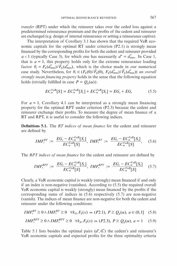
OPTIMAL REINSURANCE REVISITED 567
transfer (RPT) under which the reinsurer takes over the ceded loss against a predetermined reinsurance premium and the profi ts of the cedent and reinsurer are exchanged (e.g. design of internal reinsurance or setting a reinsurance captive).
The interpretation of Corollary 3.1 has shown that the required VaR eco-nomic capitals for the optimal RT under criterion (P2.1) is strongly mean fi nanced by the corresponding profi ts for both the cedent and reinsurer provided a 1< (typically Case 3), for which one has necessarily d maxd* = * . In Case 1, that is a 1= , this property holds only for the extreme reinsurance loading factor r Smax max( ) ( )F d dS=q / F* * , which is the choice made in our numericalcase study. Nevertheless, for (0),r S Smax max(0) ( ) ( ))(F F d dS S!q // F F* * an overall strongly mean fi nancing property holds in the sense that the following equation holds (trivially fulfi lled in case (aS )P = Q ):
a a a[ ] [ ] [ ]EC EC EC EG EGc c rr+ +SVaR VaR VaR S= =S (5.5)
For a 1= , Corollary 4.1 can be interpreted as a strongly mean fi nancing property for the optimal RPT under criterion (P2.3) because the cedent and reinsurer exchange their profi ts. To measure the degree of mean fi nance of a RT and RPT, it is useful to consider the following indices.
Defi nitions 5.1. The RT indices of mean fi nance for the cedent and reinsurer are defi ned by
= =rc : :a
a
a
a
[ ][ ]
,[ ]
[ ],IMF
ECEG EC
IMFEC
EG ECc c r- - rVaR
VaR
VaR
VaRRT RT
S SS S
(5.6)
The RPT indices of mean fi nance for the cedent and reinsurer are defi ned by
= =rc : :a
a
a
a
[ ][ ]
,[ ]
[ ]IMF
ECEG EC
IMFEC
EG ECcRPT r RPT c- - rVaR
VaR
VaR
VaR
S SS S
(5.7)
Clearly, a VaR economic capital is weakly (strongly) mean fi nanced if and only if an index is non-negative (vanishes). According to (5.5) the required overall VaR economic capital is weakly (strongly) mean fi nanced by the profi ts if the corresponding sums of indices in (5.6) respectively (5.7) are non-negative(vanish). The indices of mean fi nance are non-negative for both the cedent and reinsurer under the following conditions:
(c r aS, (k (x PS60 0 ) 2.1), ), (0,1]IMF IMF F P aS +/$ $ $ !RT RT Q (5.8)
(c r aS, (k (x PS6 ) . ), ),IMF IMF F P a0 0 2 3 1S +/$ $ $ =RPT RPT Q (5.9)
Table 5.1 lists besides the optimal pairs , qrd( )* * the cedent’s and reinsurer’s VaR economic capitals and expected profi ts for the three optimality criteria
94838_Astin41-2_10_Hurlimann.indd 56794838_Astin41-2_10_Hurlimann.indd 567 2/12/11 08:332/12/11 08:33

568 W. HÜRLIMANN
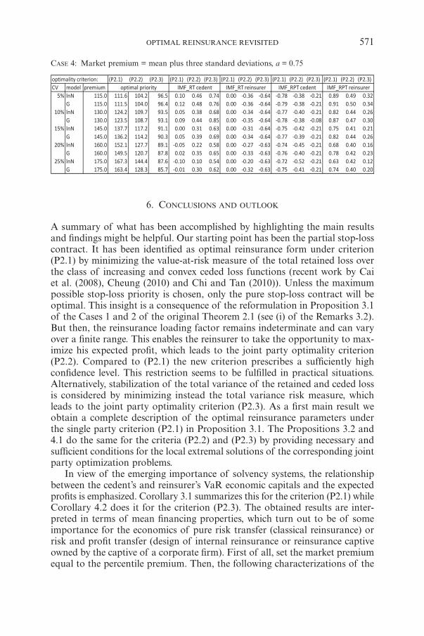
under the four Cases. Table 5.2 displays the corresponding indices of mean fi nance. The abbreviation CV for coeffi cient of variation is used in the Tables and discussion.
The most important properties and dependencies can be read off from the Tables as follows:
(1) The optimal pairs , qrd( )* * depend on the loss distribution but not on the market premium, and depend on the partial stop-loss factor a only under (P2.3). For criterion (P2.1) the values of , rd q* * are the highest possible ones (extreme reinsurance loading factor) but any other values satisfying
qrd max0 ( )d d< * #= * * could have been chosen as already explained in the text.
(2) The optimal pairs , qrd( )* * for criterion (P2.1) are similar for the lognormal and gamma distributions. For the criteria (P2.2)-(P2.3) they differ more and more by increasing CV. In particular, qr
* increases much faster under a lognormal distribution than under a gamma distribution by increasing CV for the criterion (P2.2).
(3) The optimal priority is increasing with increasing CV except for criterion (P2.3), a = 0.75. In this situation it is decreasing with increasing CV.
(4) The optimal reinsurance loading factor is increasing with increasing CV for the criteria (P2.2)-(P2.3), but it is decreasing with increasing CV for criterion (P2.1).
(5) The properties of the optimal priority solving the equation (C3.1) for criterion (P2.3) are instructive. In case a 1= the optimal priority is close to the mean but above it, in agreement with Case 1 of Proposition 4.2 and the observations already made in former papers (e.g. Hürlimann (1994b), Hürlimann (1999), Section 4). For ( , ]a 12
1! the optimal priority is less
than the mean, in agreement with Case 2 of Proposition 4.2. One can argue that a priority less than the mean is not meaningful, as donein Hürlimann(1999), hence only the pure stop-loss case a 1= might be practical.
(6) For fi xed a the VaR economic capitals of the cedent and reinsurer aswell as the reinsurer’s expected profi ts do not depend upon the market premium but depend on the loss distribution. The expected profi t ofthe cedent depends on a, the market premium and the loss distribution. Maximizing the reinsurer’s expected profi t under criterion (P2.2) requires a high increase of economic capital for a moderate increase in expected profi t when compared to criterion (P2.1). However, the corresponding reinsurance premiums are much more competitive for criterion (P2.2) in this situation (much smaller reinsurance loading factors).
(7) The overall VaR economic capital is strongly mean fi nanced by the profi ts in the Cases 1 and 3 under all criteria. Since (aS )P = Q this is a trivial property. Accordingly, in the Cases 2 and 4, the same weak property only holds for those smaller CV’s satisfying (aS )P > Q .
94838_Astin41-2_10_Hurlimann.indd 56894838_Astin41-2_10_Hurlimann.indd 568 2/12/11 08:332/12/11 08:33

OPTIMAL REINSURANCE REVISITED 569
(8) The cedant’s and reinsurer’sVaR economic capitals are strongly mean fi nanced by their own profi ts (Cases 1 and 3 for the RT under criterion (P2.1)) respectively by their exchanged profi ts (Case 1 for the RPT under criterion (P2.3)). The same weak properties hold in the Cases 2 and 4 for the RT, respectively Case 2 for the RPT, provided the CV’s are suffi ciently small to satisfy (aS )P > Q .
TABLE 5.1
ECONOMIC CAPITAL AND EXPECTED PROFIT FOR OPTIMAL PAIRS , qrd( )* *
CASE 1: Market premium = percentile premium to confi dence level 99.5%, a = 1
CASE 2: Market premium = mean plus three standard deviations, a = 1
CASE 3: Market premium = percentile premium to confi dence level 99.5%, a = 0.75
94838_Astin41-2_10_Hurlimann.indd 56994838_Astin41-2_10_Hurlimann.indd 569 2/12/11 08:332/12/11 08:33

570 W. HÜRLIMANN
CASE 4: Market premium = mean plus three standard deviations, a = 0.75
TABLE 5.2
INDICES OF MEAN SELF-FINANCE FOR OPTIMAL RT AND RPT
CASE 1: Market premium = percentile premium to confi dence level 99.5%, a = 1
CASE 3: Market premium = percentile premium to confi dence level 99.5%, a = 0.75
CASE 2: Market premium = mean plus three standard deviations, a = 1
94838_Astin41-2_10_Hurlimann.indd 57094838_Astin41-2_10_Hurlimann.indd 570 2/12/11 08:332/12/11 08:33
OPTIMAL REINSURANCE REVISITED 571
6. CONCLUSIONS AND OUTLOOK
A summary of what has been accomplished by highlighting the main results and fi ndings might be helpful. Our starting point has been the partial stop-loss contract. It has been identifi ed as optimal reinsurance form under criterion (P2.1) by minimizing the value-at-risk measure of the total retained loss over the class of increasing and convex ceded loss functions (recent work by Caiet al. (2008), Cheung (2010) and Chi and Tan (2010)). Unless the maximum possible stop-loss priority is chosen, only the pure stop-loss contract will be optimal. This insight is a consequence of the reformulation in Proposition 3.1 of the Cases 1 and 2 of the original Theorem 2.1 (see (i) of the Remarks 3.2). But then, the reinsurance loading factor remains indeterminate and can vary over a fi nite range. This enables the reinsurer to take the opportunity to max-imize his expected profi t, which leads to the joint party optimality criterion (P2.2). Compared to (P2.1) the new criterion prescribes a suffi ciently high confi dence level. This restriction seems to be fulfi lled in practical situations. Alternatively, stabilization of the total variance of the retained and ceded loss is considered by minimizing instead the total variance risk measure, which leads to the joint party optimality criterion (P2.3). As a fi rst main result we obtain a complete description of the optimal reinsurance parameters under the single party criterion (P2.1) in Proposition 3.1. The Propositions 3.2 and 4.1 do the same for the criteria (P2.2) and (P2.3) by providing necessary and suffi cient conditions for the local extremal solutions of the corresponding joint party optimization problems.
In view of the emerging importance of solvency systems, the relationship between the cedent’s and reinsurer’s VaR economic capitals and the expected profi ts is emphasized. Corollary 3.1 summarizes this for the criterion (P2.1) while Corollary 4.2 does it for the criterion (P2.3). The obtained results are inter-preted in terms of mean fi nancing properties, which turn out to be of some importance for the economics of pure risk transfer (classical reinsurance) or risk and profi t transfer (design of internal reinsurance or reinsurance captive owned by the captive of a corporate fi rm). First of all, set the market premium equal to the percentile premium. Then, the following characterizations of the
CASE 4: Market premium = mean plus three standard deviations, a = 0.75
94838_Astin41-2_10_Hurlimann.indd 57194838_Astin41-2_10_Hurlimann.indd 571 2/12/11 08:332/12/11 08:33

572 W. HÜRLIMANN
GRAPH 6.1: Comparison of the pure stop-loss optimal risk transfer strategies
optimal risk transfer strategies can be formulated (consequences of the Corol-laries 3.1 and 4.1):
(1) Consider an optimal pure risk transfer agreement under criterion (P2.1). The cedent’s and reinsurer’s required VaR economic capitals are both strongly mean fi nanced by their profi ts, if and only if, the maximum optimal stop-loss priority is chosen. Moreover, in this situation, the cedent’s VaR economic capital is minimum and the reinsurer’s expected profi t is maximum only for the pure stop-loss contract.
(2) Consider an optimal risk and profi t transfer agreement under criterion (P2.3). The cedent’s and reinsurer’s required VaR economic capitals are both strongly mean fi nanced by their exchanged profi ts, if and only if, the pure stop-loss contract is chosen. Moreover, in this situation, the cedent’s VaR economic capital is minimum and the total variance of the retained and ceded loss is minimum.
To illustrate, assume a percentile market premium and that the characterizing property in (1) and (2) holds. It is remarkable to observe additionally thatthe optimal cedent’s and reinsurer’s expected profi ts under the criteria (P2.1) and (P2.3) are very close, especially for the lower coeffi cients of variation.The Graph 6.1 illustrates this fi nding for the lognormal insurance loss distribution. The big difference lies in the optimal priorities and reinsurance loading factors,
94838_Astin41-2_10_Hurlimann.indd 57294838_Astin41-2_10_Hurlimann.indd 572 2/12/11 08:332/12/11 08:33

OPTIMAL REINSURANCE REVISITED 573
which turn out to be much larger under criterion (P2.1). In particular, higher retained VaR economic capitals are required under (P2.1).
Finally, on cannot conclude without giving a brief outlook for possible work. Besides the CVaR risk measure, also called tail conditional expectation (CTE) risk measure, other important risk measures can be considered. For example, in the class of tail preserving risk measures, one fi nds the right-tail risk measure by Wang (1998) (see also Hürlimann (2004)) and the lookback risk measure (e.g. Hürlimann (1998/2003/2004)). Future research on this topic should include other optimal reinsurance forms like the limited and truncated stop-loss contracts (comments of Section 2) and the excess-of-loss reinsurance contract studied in Meng and Zhang (2010).
ACKNOWLEGEMENTS
The author is very grateful to the referees for careful reading, helpful comments and suggestions for improved proofs, results and presentation.
REFERENCES
ARROW, K. (1963) Uncertainty and the Welfare Economics of Medical Care. The American Economic Review 53, 941-73.
ARROW, K. (1974) Optimal Insurance and Generalized Deductibles. Scandinavian Actuarial Journal, 1-42.
BERNARD, C. and TIAN, W. (2009) Optimal reinsurance arrangements under tail risk measures. Journal of Risk and Insurance 76(3), 709-725.
BORCH, K.H. (1960) An attempt to determine the optimum amount of stop-loss reinsurance. Transactions of the 16th International Congress of Actuaries, 2, 579-610.
BORCH, K.H. (1969) The optimal reinsurance treaty. ASTIN Bulletin 5(2), 293-297.BORCH, K.H. (1990) Economics of Insurance. Advanced Textbooks in Economics, 29. North-
Holland.BOWERS, N.L. (1969) An upper bound for the net stop-loss premium. Transactions of the Society
of Actuaries XIX, 211-216.CAI, J. and TAN, K.S. (2007) Optimal retention for a stop-loss reinsurance under the VaR and
CTE risk measures. ASTIN Bulletin 37(1), 93-112.CAI, J., TAN, K.S., WENG, C. and ZHANG, Y. (2008) Optimal reinsurance under VaR and CTE
risk measures. Insurance: Mathematics and Economics 43, 185-196.CHI, Y. and TAN, K.S. (2010) Optimal reinsurance under VaR and CVaR risk measures: a simpli-
fi ed approach. Working paper SSRN id=1578622.CHEUNG, K.C. (2010) Optimal reinsurance revisited – a geometric approach. ASTIN Bulletin 40(1),
221-239.CUMMINS, J.D. and MAHUL, O. (2004) The demand for insurance with an upper limit on cover-
age. The Journal of Risk and Insurance 71(2), 253-264.DIMITROVA, D.S. and KAISHEV, V.K. (2010) Optimal joint survival reinsurance: an effi cient fron-
tier approach. Insurance: Mathematics and Economics 47(1), 27-35.GAJEK, L. and ZAGRODNY, D. (2004a) Optimal reinsurance under general risk measures. Insur-
ance: Mathematics and Economics 34(2), 227-240.GAJEK, L. and ZAGRODNY, D. (2004b) Reinsurance arrangements maximizing insurer’s survival
probability. The Journal of Risk and Insurance 71(3), 421-435.HÜRLIMANN, W. (1994a) Splitting risk and premium calculation. Bulletin of the Swiss Association
of Actuaries, 167-97.
94838_Astin41-2_10_Hurlimann.indd 57394838_Astin41-2_10_Hurlimann.indd 573 2/12/11 08:332/12/11 08:33

574 W. HÜRLIMANN
HÜRLIMANN, W. (1994b) From the inequalities of Bowers, Kremer and Schmitter to the total stop-loss risk. Proceedings 25th International ASTIN Colloquium, Cannes.
HÜRLIMANN, W. (1996) Mean-variance portfolio theory under portfolio insurance. In: Albrecht, P. (Ed.). Aktuarielle Ansätze für Finanz-Risiken. Proceedings 6th International AFIR Collo-quium, Nürnberg, vol. 1, 347-374. Verlag Versicherungswirtschaft, Karlsruhe.
HÜRLIMANN, W. (1997a) An elementary unifi ed approach to loss variance bounds. Bulletin of the Swiss Association of Actuaries, 73-88.
HÜRLIMANN, W. (1997b). Fonctions extrémales et gain fi nancier. Elemente der Math. 52, 152-168.HÜRLIMANN, W. (1998) Inequalities for lookback option strategies and exchange risk modelling.
Proc. 1st Euro-Japanese Workshop on Stochastic Risk Modelling for Insurance, Finance, Production and Reliability. Available at http://sites.google.com/site/whurlimann/
HÜRLIMANN, W. (1999) Non-optimality of a linear combination of proportional and non-proportional reinsurance. Insurance: Mathematics and Economics 24, 219-227.
HÜRLIMANN, W. (2000) Higher-degree stop-loss transforms and stochastic orders (I) theory. Blätter der Deutschen Gesellschaft für Versicherungsmathematik XXIV(3), 449-463.
HÜRLIMANN, W. (2002) Economic risk capital allocation from top down. Blätter der Deutschen Gesellschaft für Versicherungsmathematik 25(4), 885-891.
HÜRLIMANN, W. (2003) An economic risk capital allocation for lookback fi nancial losses. Available at http://sites.google.com/site/whurlimann/
HÜRLIMANN, W. (2004) Distortion risk measures and economic capital. North American Actuarial Journal 8(1), 86-95.
HÜRLIMANN, W. (2010) Case study on the optimality of some reinsurance contracts. Bulletin of the Swiss Association of Actuaries, 2, 71-91.
IGNATOV, Z.G., KAISHEV, V.K. and KRACHUNOV, R.S. (2004) Optimal retention levels, given the joint survival of cedent and reinsurer. Scandinavian Acturarial Journal 6, 401-430.
KAHN, P.M. (1961) Some remarks on a recent paper by Borch. ASTIN Bulletin 1(5), 265-72.KAISHEV, V.K. and DIMITROVA, D.S. (2006). Excess of loss reinsurance under joint survival
optimality. Insurance: Mathematics and Economics 39(3), 376-389.KALUSZKA, M. (2005) Truncated stop-loss as optimal reinsurance agreement in one-period models.
ASTIN Bulletin 35(2), 337-349.KALUSZKA, M. and OKOLEWSKI, A. (2008) An extension of Arrow’s result on optimal reinsurance
contract. Journal of Risk and Insurance 75(2), 275-288.KREMER, E. (1990) An elementary upper bound for the loading of a stop-loss cover. Scandinavian
Actuarial Journal, 105-108.MENG, H. and ZHANG, X. (2010) Optimal risk control for the excess of loss reinsurance policies.
ASTIN Bulletin 40(1), 179-197.OHLIN, J. (1969) On a class of measures of dispersion with application to optimal reinsurance.
ASTIN Bulletin 5, 249-66.VAJDA, S. (1962) Minimum variance reinsurance. ASTIN Bulletin 2(2), 257-260.VENTER, C.G. (2001) Measuring value in reinsurance. Seminar on Reinsurance, Handouts, Casualty
Actuarial Society, http://www.casact.net/pubs/forum/01sforum/01sf179.pdfWANG, S. (1998) An actuarial index of the right-tail risk. North American Actuarial Journal 2(2),
88-101.
WERNER HÜRLIMANN
FRSGlobal SwitzerlandSeefeldstrasse 69CH-8008 ZürichE-mail: [email protected]: http://sites.google.com/site/whurlimann/
94838_Astin41-2_10_Hurlimann.indd 57494838_Astin41-2_10_Hurlimann.indd 574 2/12/11 08:332/12/11 08:33