Embed Size (px)
Citation preview
Journal of Macroeconomics 26 (2004) 183–209
www.elsevier.com/locate/econbase
Optimal fiscal and monetary policyunder imperfect competition
Stephanie Schmitt-Groh�e a,c,d,*, Mart�ın Uribe b,d
a Department of Economics, Rutgers University, New Brunswick, NJ 08901, USAb Department of Economics, University of Pennsylvania, Philadelphia, PA 19104, USA
c NBER, Cambridge, MA, USAd CEPR, London, UK
Received 21 April 2003; accepted 1 August 2003
Available online 7 January 2004
Abstract
This paper studies optimal fiscal and monetary policy under imperfect competition in a sto-
chastic, flexible-price, production economy without capital. It shows analytically that in this
economy the nominal interest rate acts as an indirect tax on monopoly profits. Unless the so-
cial planner has access to a direct 100% tax on profits, he will always find it optimal to deviate
from the Friedman rule by setting a positive and time-varying nominal interest rate. The dy-
namic properties of the Ramsey allocation are characterized numerically. As in the perfectly
competitive case, the labor income tax is remarkably smooth, whereas inflation is highly vol-
atile and serially uncorrelated. An exact numerical solution method to the Ramsey conditions
is proposed.
� 2003 Elsevier Inc. All rights reserved.
JEL classification: E52; E61; E63
Keywords: Optimal fiscal and monetary policy; Imperfect competition; Friedman rule; Profit taxes
1. Introduction
In the existing literature on optimal monetary policy two distinct branches have
developed that deliver diametrically opposed policy recommendations concerning
* Corresponding author. Address: Department of Economics, Duke University, P.O. Box 90097,
Durham, NC 27708, USA. Tel.: +1-919-660-1889; fax: +1-919-684-8974.
E-mail addresses: [email protected], [email protected] (S. Schmitt-Groh�e), [email protected].
edu (M. Uribe).
0164-0704/$ - see front matter � 2003 Elsevier Inc. All rights reserved.
doi:10.1016/j.jmacro.2003.11.002
184 S. Schmitt-Groh�e, M. Uribe / Journal of Macroeconomics 26 (2004) 183–209
the long-run and cyclical behavior of prices and interest rates. One branch follows
the theoretical framework laid out in Lucas and Stokey (1983). It studies the joint
determination of optimal fiscal and monetary policy in flexible-price environments
with perfect competition in product and factor markets. In this group of papers,
the government’s problem consists in financing an exogenous stream of publicspending by choosing the least disruptive combination of inflation and distortionary
income taxes. The criterion under which policies are evaluated is the welfare of the
representative private agent. A basic result of this literature is the optimality of the
Friedman rule. A zero opportunity cost of money has been shown to be optimal
under perfect-foresight in a variety of monetary models, including cash-in-advance,
money-in-the-utility function, and shopping-time models. 1
In a significant contribution to the literature, Chari et al. (1991) characterize opti-
mal monetary and fiscal policy in stochastic environments. They prove that theFriedman rule is also optimal under uncertainty: the government finds it optimal
to set the nominal interest rate at zero at all dates and all states of the world. In addi-
tion, Chari et al. show that income tax rates are remarkably stable over the business
cycle, and that the inflation rate is highly volatile and serially uncorrelated. Under
the Ramsey policy, the government uses unanticipated inflation as a lump-sum tax
on financial wealth. The government is able to do this because public debt is assumed
to be nominal and non-state-contingent. Thus, inflation plays the role of a shock ab-
sorber of unexpected adverse fiscal shocks.On the other hand, a more recent literature focuses on characterizing optimal
monetary policy in environments with nominal rigidities and imperfect competi-
tion. 2 Besides its emphasis on the role of price rigidities and market power, this lit-
erature differs from the earlier one described above in two important ways. First, it
assumes, either explicitly or implicitly, that the government has access to (endoge-
nous) lump-sum taxes to finance its budget. An important implication of this
assumption is that there is no need to use unanticipated inflation as a lump-sum
tax; regular lump-sum taxes take up this role. Second, the government is assumedto be able to implement a production (or employment) subsidy so as to eliminate
the distortion introduced by the presence of monopoly power in product and factor
markets.
A key result of this literature is that the optimal monetary policy features an infla-
tion rate that is zero or close to zero at all dates and all states. 3 In addition, the nom-
inal interest rate is not only different from zero, but also varies significantly over the
1 See, for example, Chari et al. (1991), Correia and Teles (1996), Guidotti and V�egh (1993), and
Kimbrough (1986).2 See, for example, Erceg et al. (2000), Gal�ı and Monacelli (2000), Khan et al. (2000), and Rotemberg
and Woodford (1999).3 In models where money is used exclusively as a medium of account or when money enters in an
additively separable way in the utility function, the optimal inflation rate is typically strictly zero. Khan
et al. (2000) show that when a non-trivial transaction role for money is introduced, the optimal inflation
rate lies between zero and the one called for by the Friedman rule. However, in calibrated model
economies, they find that the optimal rate of inflation is in fact very close to zero and smooth.
S. Schmitt-Groh�e, M. Uribe / Journal of Macroeconomics 26 (2004) 183–209 185
business cycle. The reason why price stability turns out to be optimal in environ-
ments of the type described here is straightforward: the government keeps the price
level constant in order to minimize (or completely eliminate) the costs introduced by
inflation under nominal rigidities.
This paper is the first step of a larger research project that aims to incorporate in aunified framework the essential elements of the two approaches to optimal policy de-
scribed above. Specifically, in this paper we build a model that shares three elements
with the earlier literature: (a) The only source of regular taxation available to the
government is distortionary income taxes. In particular, the fiscal authority cannot
adjust lump-sum taxes endogenously in financing its outlays. (b) Prices are fully flex-
ible. (c) The government cannot implement production subsidies to undo distortions
created by the presence of imperfect competition. At the same time, our model shares
with the more recent body of work on optimal monetary policy the assumption thatproduct markets are not perfectly competitive. In particular, we assume that each
firm in the economy is the monopolistic producer of a differentiated good. An
assumption maintained throughout this paper that is common to all of the papers
cited above (except for Lucas and Stokey, 1983) is that the government has the abil-
ity to fully commit to the implementation of announced fiscal and monetary policies.
In our imperfectly competitive economy, profits represent the income to a fixed
‘‘factor,’’ namely, monopoly rights. It is therefore optimal for the Ramsey planner
to tax profits at a 100% rate. Realistically, however, governments cannot implementa complete confiscation of this type of income. The main finding of our paper is that
under this restriction the Friedman rule ceases to be optimal. The Ramsey planner
resorts to a positive nominal interest rate as an indirect way to tax profits. The nom-
inal interest rate represents an indirect tax on profits because households must hold
(non-interest-bearing) fiat money in order to convert income into consumption. In-
deed, we find that the Ramsey allocation features an increasing relationship between
the nominal interest rate and monopoly profits. Under the assumption of no profit
taxation and for plausible calibrations of other structural parameters of the modeleconomy, we find that as the profit share increases from 0% to 25%, the optimal
average nominal interest rate increases continuously from 0% to 8% per year. In
addition, the interest rate is time varying and its volatility is increasing in the degree
of monopoly power.
The second central result of our study is that while the first moments of inflation,
the nominal interest rate, and tax rates are sensitive to the degree of market power in
the Ramsey allocation, the cyclical properties of these variables under imperfect
competition are similar to those arising in perfectly competitive environments. Inparticular, it is optimal for the government to smooth tax rates and to make the
inflation rate highly volatile. Thus, as in the case of perfect competition, the govern-
ment uses variations in the price level as a state-contingent tax on financial wealth.
The remainder of the paper is organized in five sections. Section 2 describes the eco-
nomic environment and defines a competitive equilibrium. Section 3 presents the pri-
mal form of the equilibrium and shows that it is equivalent to the definition of
competitive equilibrium given in Section 2. Section 4 establishes the first central result
of this paper. Namely, the fact that the Friedman rule is not optimal when monopoly
186 S. Schmitt-Groh�e, M. Uribe / Journal of Macroeconomics 26 (2004) 183–209
profits cannot be fully confiscated. Section 5 analyzes the business-cycle properties of
Ramsey allocations. It first presents a novel numerical method for solving the exact
conditions of the Ramsey problem. It then describes the calibration of the model
and presents the quantitative results. Section 6 presents some concluding remarks.
2. The model
In this section we develop a simple infinite-horizon production economy with
imperfectly competitive product markets. Prices are assumed to be fully flexible
and asset markets complete. The government finances an exogenous stream of pur-
chases by levying distortionary income taxes and printing money.
2.1. The private sector
Consider an economy populated by a large number of identical households. Each
household has preferences defined over processes of consumption and leisure and de-
scribed by the utility function
E0
X1t¼0
btUðct; htÞ; ð1Þ
where ct denotes consumption, ht denotes labor effort, b 2 ð0; 1Þ denotes the sub-
jective discount factor, and E0 denotes the mathematical expectation operator con-
ditional on information available in period 0. The single-period utility function U is
assumed to be increasing in consumption, decreasing in effort, strictly concave, and
twice continuously differentiable.
In each period tP 0, households can purchase two types of financial assets: fiat
money, Mt, and one-period, state-contingent, nominal assets, Dtþ1, that pay one unit
of currency in a particular state of period t þ 1. Money holdings are motivated byassuming that they facilitate consumption purchases. Specifically, consumption pur-
chases are subject to a proportional transaction cost sðvtÞ that depends on the house-
hold’s money-to-consumption ratio, or consumption-based money velocity,
vt ¼PtctMt
; ð2Þ
where Pt denotes the price of the consumption good in period t. The transaction cost
function satisfies the following assumption:
Assumption 1. The function sðvÞ satisfies: (a) sðvÞ is non-negative and twice contin-
uously differentiable; (b) there exists a level of velocity v > 0, to which we refer as the
satiation level of money, such that sðvÞ ¼ s0ðvÞ ¼ 0; (c) ðv� vÞs0ðvÞ > 0 for v 6¼ v; and(d) 2s0ðvÞ þ vs00ðvÞ > 0 for all vP v.
Assumption 1(a) states that the transaction cost is smooth. Assumption 1(b) en-
sures that the Friedman rule, i.e., a zero nominal interest rate, need not be associated
S. Schmitt-Groh�e, M. Uribe / Journal of Macroeconomics 26 (2004) 183–209 187
with an infinite demand for money. It also implies that both the transaction cost and
the distortion it introduces vanish when the nominal interest rate is zero. Assump-
tion 1(c) guarantees that money velocity is always greater than or equal to the sati-
ation level. As will become clear shortly, Assumption 1(d) ensures that the demand
for money is decreasing in the nominal interest rate. (Note that Assumption 1(d) isweaker than the more common assumption of strict convexity of the transaction cost
function.)
The consumption good ct is assumed to be a composite good made of a
continuum of intermediate differentiated goods. The aggregator function is of the
Dixit–Stiglitz type. Each household is the monopolistic producer of one variety of
intermediate goods. The intermediate goods are produced using a linear technology,
zt~ht, that takes labor, ~ht, as the sole input and is subject to an exogenous productivity
shock, zt. The household hires labor from a perfectly competitive market. The de-mand for the intermediate input is of the form YtdðptÞ, where Yt denotes the level
of aggregate demand and pt denotes the relative price of the intermediate good in
terms of the composite consumption good. The demand function dð�Þ is assumed
to be decreasing and to satisfy dð1Þ ¼ 1 and d 0ð1Þ < �1. 4 The monopolist sets the
price of the good it supplies taking the level of aggregate demand as given, and is
constrained to satisfy demand at that price, that is,
4 Th
zt~ht P YtdðptÞ: ð3Þ
Finally, we assume that each period the household receives profits from financialinstitutions in the amount Pt. The household takes Pt as exogenous. We introducethe variablePt because we want to allow for the possibility that in equilibrium only a
fraction of the transactions costs be true resource (or shoe-leather) costs. We do so
by assuming that part of the transaction cost is rebated to the public in a lump-sum
fashion. We motivate this rebate by assuming that part of the transaction cost rep-
resent pure profits of financial institutions owned (in equal shares) by the public.
The flow budget constraint of the household in period t is then given by
Ptct½1þ sðvtÞ� þMt þ Etrtþ1Dtþ1 6Mt�1 þ Dt þ Pt½ptYtdðptÞ � wt~ht�
þ ð1� stÞPtwtht þPt; ð4Þ
where wt is the real wage rate and st is the labor income tax rate. The variable rtþ1
denotes the period-t price of a claim to one unit of currency in a particular state of
period t þ 1 divided by the probability of occurrence of that state conditional oninformation available in period t. The left-hand side of the budget constraint rep-
resents the uses of wealth: consumption spending, including transactions costs,
money holdings, and purchases of interest-bearing assets. The right-hand side shows
the sources of wealth: money and contingent claims acquired in the previous period,
profits from the sale of the differentiated good, after-tax labor income, and profits
received from financial institutions.
e restrictions on dð1Þ and d 0ð1Þ are necessary for the existence of a symmetric equilibrium.
188 S. Schmitt-Groh�e, M. Uribe / Journal of Macroeconomics 26 (2004) 183–209
In addition, the household is subject to the following borrowing constraint that
prevents it from engaging in Ponzi schemes:
limj!1
Etqtþjþ1ðDtþjþ1 þMtþjÞP 0; ð5Þ
at all dates and under all contingencies. The variable qt represents the period-zero
price of one unit of currency to be delivered in a particular state of period t dividedby the probability of occurrence of that state given information available at time 0
and is given by
qt ¼ r1r2 � � � rt
with q0 � 1.The household chooses the set of processes fct; ht; ~ht; pt; vt;Mt;Dtþ1g1t¼0, so as to
maximize (1) subject to (2)–(5), taking as given the set of processes fYt; Pt;wt;rtþ1; st; ztg1t¼0 and the initial condition M�1 þ D0.
Let the multiplier on the flow budget constraint be kt=Pt. Then the first-order con-
ditions of the household’s maximization problem are (2)–(5) holding with equality
and
Ucðct; htÞ ¼ kt½1þ sðvtÞ þ vts0ðvtÞ�; ð6Þ
�Uhðct; htÞUcðct; htÞ
¼ ð1� stÞwt
1þ sðvtÞ þ vts0ðvtÞ; ð7Þ
v2t s0ðvtÞ ¼ 1� Etrtþ1; ð8Þ
ktPtrtþ1 ¼ b
ktþ1
Ptþ1
; ð9Þ
pt þdðptÞd 0ðptÞ
¼ wt
zt: ð10Þ
The interpretation of these optimality conditions is straightforward. The first-order
condition (6) states that the transaction cost introduces a wedge between the mar-
ginal utility of consumption and the marginal utility of wealth. The assumed form of
the transaction cost function ensures that this wedge is zero at the satiation point vand increasing in money velocity for v > v. Eq. (7) shows that both the labor income
tax rate and the transaction cost distort the consumption/leisure margin. Given the
wage rate, households will tend to work less and consume less the higher is s or thesmaller is vt. Eq. (8) implicitly defines the household’s money demand function. Notethat Etrtþ1 is the period-t price of an asset that pays one unit of currency in every
state in period t þ 1. Thus Etrtþ1 represents the inverse of the risk-free gross nominal
interest rate. Formally, letting Rt denote the gross risk-free nominal interest rate,
we have
Rt ¼1
Etrtþ1
:
S. Schmitt-Groh�e, M. Uribe / Journal of Macroeconomics 26 (2004) 183–209 189
Our assumptions about the form of the transactions cost function imply that the
demand for money is strictly decreasing in the nominal interest rate and unit elastic
in consumption. Eq. (9) represents a standard pricing equation for one-step-ahead
nominal contingent claims. Finally, Eq. (10) states that firms set prices so as to
equate marginal revenue, pt þ dðptÞ=d 0ðptÞ, to marginal cost, wt=z.
2.2. The government
The government faces a stream of public consumption, denoted by gt, that is
exogenous, stochastic, and unproductive. These expenditures are financed by levying
labor income taxes at the rate st, by printing money, and by issuing one-period, risk-
free, nominal obligations, which we denote by Bt. The government’s sequential bud-
get constraint is then given by
Mt þ Bt ¼ Mt�1 þ Rt�1Bt�1 þ Ptgt � stPtwtht
for tP 0. The monetary/fiscal regime consists in the announcement of state-con-
tingent plans for the nominal interest rate and the tax rate, fRt; stg.
2.3. Equilibrium
We restrict attention to symmetric equilibria where all households charge the
same price for the good they produce. As a result, we have that pt ¼ 1 for all t. Itthen follows from the fact that all firms face the same wage rate, the same technology
shock, and the same production technology, that they all hire the same amount of
labor. That is, ~ht ¼ ht. Also, because all firms charge the same price, we have that
the marginal revenue of the individual monopolist, given by the left-hand side of
(10), is constant and equal to 1þ 1=d 0ð1Þ. Letting
g ¼ d 0ð1Þdenote the equilibrium value of the elasticity of demand faced by the monopolist and
l the equilibrium gross markup of prices to marginal cost, we have that
l ¼ g1þ g
: ð11Þ
The equilibrium gross markup approaches unity as the demand elasticity becomes
perfectly elastic (g ! �1) and approaches infinity as the demand elasticity becomes
unit elastic (g ! �1).
Because all households are identical, in equilibrium there is no borrowing or lend-
ing among them. Thus, all interest-bearing asset holdings by private agents are in the
form of government securities. That is,
Dt ¼ Rt�1Bt�1
at all dates and all contingencies. In equilibrium, it must be the case that the nominal
interest rate is non-negative,
Rt P 1:
190 S. Schmitt-Groh�e, M. Uribe / Journal of Macroeconomics 26 (2004) 183–209
Otherwise pure arbitrage opportunities would exist and households’ demand for
consumption would not be well defined.
Finally, as explained earlier, we assume that only a fraction a 2 ½0; 1� of the trans-action cost represents a true resource cost. The rest of the costs are assumed to be
pure profits of financial institutions owned by the public. Thus, in equilibrium
Pt ¼ ð1� aÞctsðvtÞ:
We are now ready to define an equilibrium. A competitive equilibrium as a set of
plans fct; ht;Mt;Bt; vt;wt; kt; Pt; qt; rtþ1g satisfying the following conditions:
Ucðct; htÞ ¼ kt½1þ sðvtÞ þ vts0ðvtÞ�; ð12Þ
�Uhðct; htÞUcðct; htÞ
¼ ð1� stÞwt
1þ sðvtÞ þ vts0ðvtÞ; ð13Þ
v2t s0ðvtÞ ¼
Rt � 1
Rt; ð14Þ
ktrtþ1 ¼ bktþ1
PtPtþ1
; ð15Þ
Rt ¼1
Etrtþ1
P 1; ð16Þ
1þ gg
¼ wt
zt; ð17Þ
Mt þ Bt þ stPtwtht ¼ Rt�1Bt�1 þMt�1 þ Ptgt; ð18Þ
limj!1
Etqtþjþ1ðRtþjBtþj þMtþjÞ ¼ 0; ð19Þ
qt ¼ r1r2 � � � rt with q0 ¼ 1; ð20Þ
½1þ asðvtÞ�ct þ gt ¼ ztht; ð21Þ
vt ¼ Ptct=Mt; ð22Þ
given policies fRt; stg, exogenous processes fzt; gtg, and the initial condition.
R�1B�1 þM�1. The optimal fiscal and monetary policy is the process fRt; stg asso-
ciated with the competitive equilibrium that yields the highest level of utility to the
representative household, that is, that maximizes (1). As is well known, the planner
will always find it optimal to confiscate the entire initial financial wealth of the
household by choosing a policy consistent with an infinite initial price level, P0 ¼ 1.This is because such a confiscation amounts to a non-distortionary lump-sum tax.
To avoid this unrealistic feature of optimal policy, we restrict the initial price level to
be arbitrarily given.
S. Schmitt-Groh�e, M. Uribe / Journal of Macroeconomics 26 (2004) 183–209 191
To find the optimal policy, it is convenient to use a simpler representation of the
competitive equilibrium known as the primal form. We turn to this task next.
3. Ramsey allocations
In this section we analytically derive the first central result of this paper. Namely,
that the Friedman rule ceases to be optimal when product markets are imperfectly
competitive. We begin by deriving the primal form of the competitive equilibrium.
Then we state the Ramsey problem. And finally we characterize optimal fiscal and
monetary policy.
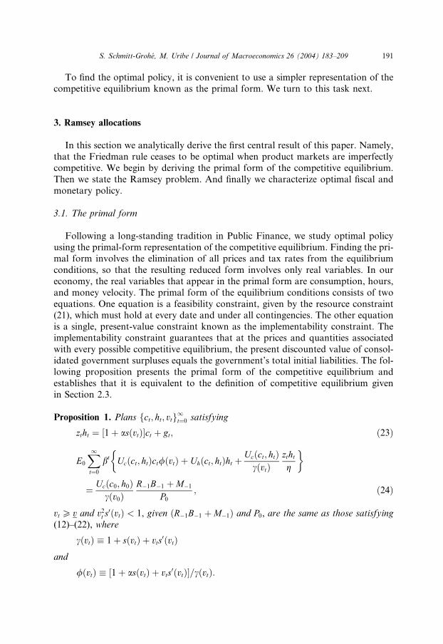
3.1. The primal form
Following a long-standing tradition in Public Finance, we study optimal policy
using the primal-form representation of the competitive equilibrium. Finding the pri-
mal form involves the elimination of all prices and tax rates from the equilibrium
conditions, so that the resulting reduced form involves only real variables. In our
economy, the real variables that appear in the primal form are consumption, hours,
and money velocity. The primal form of the equilibrium conditions consists of two
equations. One equation is a feasibility constraint, given by the resource constraint(21), which must hold at every date and under all contingencies. The other equation
is a single, present-value constraint known as the implementability constraint. The
implementability constraint guarantees that at the prices and quantities associated
with every possible competitive equilibrium, the present discounted value of consol-
idated government surpluses equals the government’s total initial liabilities. The fol-
lowing proposition presents the primal form of the competitive equilibrium and
establishes that it is equivalent to the definition of competitive equilibrium given
in Section 2.3.
Proposition 1. Plans fct; ht; vtg1t¼0 satisfying
ztht ¼ ½1þ asðvtÞ�ct þ gt; ð23Þ
E0
X1t¼0
bt Ucðct; htÞct/ðvtÞ�
þ Uhðct; htÞht þUcðct; htÞcðvtÞ
zthtg
�
¼ Ucðc0; h0Þcðv0Þ
R�1B�1 þM�1
P0; ð24Þ
vt P v and v2t s0ðvtÞ < 1, given ðR�1B�1 þM�1Þ and P0, are the same as those satisfying
(12)–(22), where
cðvtÞ � 1þ sðvtÞ þ vts0ðvtÞ
and/ðvtÞ � ½1þ asðvtÞ þ vts0ðvtÞ�=cðvtÞ:
192 S. Schmitt-Groh�e, M. Uribe / Journal of Macroeconomics 26 (2004) 183–209
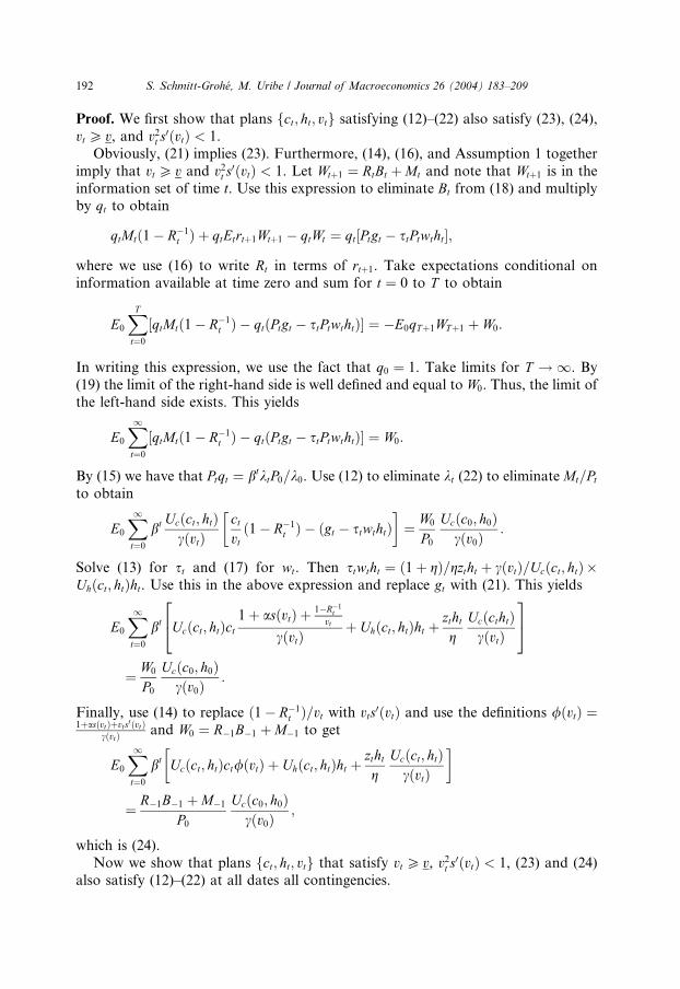
Proof. We first show that plans fct; ht; vtg satisfying (12)–(22) also satisfy (23), (24),
vt P v, and v2t s0ðvtÞ < 1.
Obviously, (21) implies (23). Furthermore, (14), (16), and Assumption 1 together
imply that vt P v and v2t s0ðvtÞ < 1. Let Wtþ1 ¼ RtBt þMt and note that Wtþ1 is in the
information set of time t. Use this expression to eliminate Bt from (18) and multiplyby qt to obtain
qtMtð1� R�1t Þ þ qtEtrtþ1Wtþ1 � qtWt ¼ qt½Ptgt � stPtwtht�;
where we use (16) to write Rt in terms of rtþ1. Take expectations conditional oninformation available at time zero and sum for t ¼ 0 to T to obtain
E0
XTt¼0
½qtMtð1� R�1t Þ � qtðPtgt � stPtwthtÞ� ¼ �E0qTþ1WTþ1 þ W0:
In writing this expression, we use the fact that q0 ¼ 1. Take limits for T ! 1. By
(19) the limit of the right-hand side is well defined and equal to W0. Thus, the limit of
the left-hand side exists. This yields
E0
X1t¼0
½qtMtð1� R�1t Þ � qtðPtgt � stPtwthtÞ� ¼ W0:
By (15) we have that Ptqt ¼ btktP0=k0. Use (12) to eliminate kt (22) to eliminate Mt=Ptto obtain
E0
X1t¼0
bt Ucðct; htÞcðvtÞ
ctvtð1
�� R�1
t Þ � ðgt � stwthtÞ�¼ W0
P0
Ucðc0; h0Þcðv0Þ
:
Solve (13) for st and (17) for wt. Then stwtht ¼ ð1þ gÞ=gztht þ cðvtÞ=Ucðct; htÞ�Uhðct; htÞht. Use this in the above expression and replace gt with (21). This yields
E0
X1t¼0
bt Ucðct; htÞct1þ asðvtÞ þ 1�R�1
tvt
cðvtÞ
24 þ Uhðct; htÞht þ
zthtg
UcðcthtÞcðvtÞ
35
¼ W0
P0
Ucðc0; h0Þcðv0Þ
:
Finally, use (14) to replace ð1� R�1t Þ=vt with vts0ðvtÞ and use the definitions /ðvtÞ ¼
1þasðvtÞþvts0ðvtÞcðvtÞ and W0 ¼ R�1B�1 þM�1 to get
E0
X1t¼0
bt Ucðct; htÞct/ðvtÞ�
þ Uhðct; htÞht þzthtg
Ucðct; htÞcðvtÞ
�
¼ R�1B�1 þM�1
P0
Ucðc0; h0Þcðv0Þ
;
which is (24).
Now we show that plans fct; ht; vtg that satisfy vt P v, v2t s0ðvtÞ < 1, (23) and (24)
also satisfy (12)–(22) at all dates all contingencies.
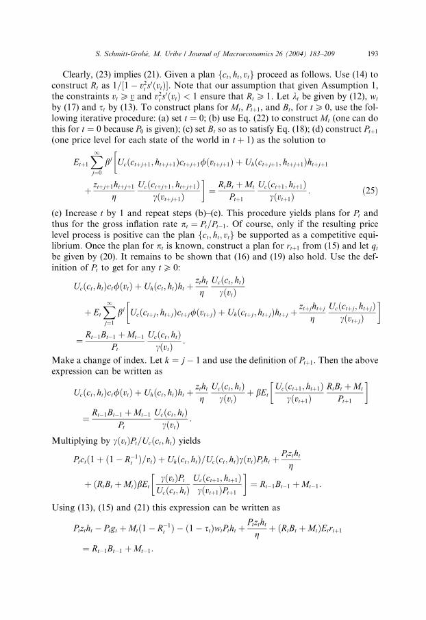
S. Schmitt-Groh�e, M. Uribe / Journal of Macroeconomics 26 (2004) 183–209 193
Clearly, (23) implies (21). Given a plan fct; ht; vtg proceed as follows. Use (14) to
construct Rt as 1=½1� v2t s0ðvtÞ�. Note that our assumption that given Assumption 1,
the constraints vt P v and v2t s0ðvtÞ < 1 ensure that Rt P 1. Let kt be given by (12), wt
by (17) and st by (13). To construct plans for Mt, Ptþ1, and Bt, for tP 0, use the fol-
lowing iterative procedure: (a) set t ¼ 0; (b) use Eq. (22) to construct Mt (one can dothis for t ¼ 0 because P0 is given); (c) set Bt so as to satisfy Eq. (18); (d) construct Ptþ1
(one price level for each state of the world in t þ 1) as the solution to
Etþ1
X1j¼0
bj Ucðctþjþ1; htþjþ1Þctþjþ1/ðvtþjþ1Þ�
þ Uhðctþjþ1; htþjþ1Þhtþjþ1
þ ztþjþ1htþjþ1
gUcðctþjþ1; htþjþ1Þ
cðvtþjþ1Þ
�¼ RtBt þMt
Ptþ1
Ucðctþ1; htþ1Þcðvtþ1Þ
: ð25Þ
(e) Increase t by 1 and repeat steps (b)–(e). This procedure yields plans for Pt andthus for the gross inflation rate pt ¼ Pt=Pt�1. Of course, only if the resulting price
level process is positive can the plan fct; ht; vtg be supported as a competitive equi-librium. Once the plan for pt is known, construct a plan for rtþ1 from (15) and let qtbe given by (20). It remains to be shown that (16) and (19) also hold. Use the def-
inition of Pt to get for any tP 0:
Ucðct; htÞct/ðvtÞ þ Uhðct; htÞht þzthtg
Ucðct; htÞcðvtÞ
þ Et
X1j¼1
bj Ucðctþj; htþjÞctþj/ðvtþjÞ�
þ Uhðctþj; htþjÞhtþj þztþjhtþj
gUcðctþj; htþjÞ
cðvtþjÞ
�
¼ Rt�1Bt�1 þMt�1
Pt
Ucðct; htÞcðvtÞ
:
Make a change of index. Let k ¼ j� 1 and use the definition of Ptþ1. Then the above
expression can be written as
Ucðct; htÞct/ðvtÞ þ Uhðct; htÞht þzthtg
Ucðct; htÞcðvtÞ
þ bEtUcðctþ1; htþ1Þ
cðvtþ1ÞRtBt þMt
Ptþ1
� �
¼ Rt�1Bt�1 þMt�1
Pt
Ucðct; htÞcðvtÞ
:
Multiplying by cðvtÞPt=Ucðct; htÞ yields
Ptctð1þ ð1� R�1t Þ=vtÞ þ Uhðct; htÞ=Ucðct; htÞcðvtÞPtht þ
Ptzthtg
þ ðRtBt þMtÞbEtcðvtÞPt
Ucðct; htÞUcðctþ1; htþ1Þcðvtþ1ÞPtþ1
� �¼ Rt�1Bt�1 þMt�1:
Using (13), (15) and (21) this expression can be written as
Ptztht � Ptgt þMtð1� R�1t Þ � ð1� stÞwtPtht þ
Ptzthtg
þ ðRtBt þMtÞEtrtþ1
¼ Rt�1Bt�1 þMt�1:
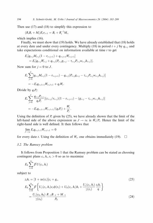
194 S. Schmitt-Groh�e, M. Uribe / Journal of Macroeconomics 26 (2004) 183–209
Then use (17) and (18) to simplify this expression to
ðRtBt þMtÞEtrtþ1 ¼ Bt þ R�1t Mt;
which implies (16).
Finally, we must show that (19) holds. We have already established that (18) holds
at every date and under every contingency. Multiply (18) in period t þ j by qtþj and
take expectations conditional on information available at time t to get
Et½qtþjMtþjð1� rtþjþ1Þ þ qtþjþ1Wtþjþ1�¼ Et½qtþjWtþj þ qtþjðPtþjgtþj � stþjPtþjwtþjhtþjÞ�:
Now sum for j ¼ 0 to J .
Et
XJ
j¼0
½qtþjMtþjð1� rtþjþ1Þ � qtþjðPtþjgtþj � stþjPtþjwtþjhtþjÞ�
¼ �EtqtþJþ1WtþJþ1 þ qtWt :
Divide by qtPt:
Et
XJ
j¼0
qtþjPtþj
qtPt½ðctþj=vtþjÞð1� rtþjþ1Þ � ðgtþj � stþjwtþjhtþjÞ�
¼ �EtqtþJþ1WtþJþ1=ðqtPtÞ þWt
Pt:
Using the definition of Pt given by (25), we have already shown that the limit of theleft-hand side of the above expression as J ! 1 is Wt=Pt. Hence the limit of the
right-hand side is well defined. It then follows that
limJ!1
EtqtþJþ1WtþJþ1 ¼ 0
for every date t. Using the definition of Wt , one obtains immediately (19). h
3.2. The Ramsey problem
It follows from Proposition 1 that the Ramsey problem can be stated as choosingcontingent plans ct; ht; vt > 0 so as to maximize
E0
X1t¼0
btUðct; htÞ
subject to
ztht ¼ ½1þ asðvtÞ�ct þ gt; ð23Þ
E0
X1t¼0
bt Ucðct; htÞct/ðvtÞ�
þ Uhðct; htÞht þUcðct; htÞcðvtÞ
zthtg
�
¼ Ucðc0; h0Þcðv0Þ
R�1B�1 þM�1
P0ð24Þ
S. Schmitt-Groh�e, M. Uribe / Journal of Macroeconomics 26 (2004) 183–209 195
and v2t s0ðvtÞ < 1, taking as given ðM�1 þ R�1B�1Þ=P0 and the exogenous stochastic
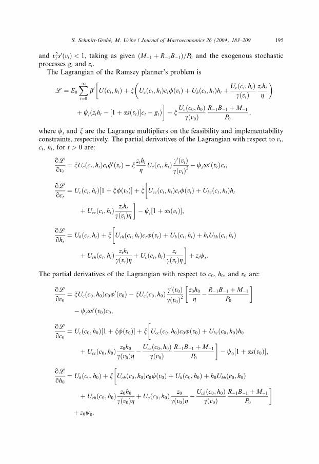
processes gt and zt.The Lagrangian of the Ramsey planner’s problem is
L ¼ E0
X1t¼0
bt Uðct; htÞ�
þ n Ucðct; htÞct/ðvtÞ�
þ Uhðct; htÞht þUcðct; htÞcðvtÞ
zthtg
�
þ wtðztht � ½1þ asðvtÞ�ct � gtÞ�� n
Ucðc0; h0Þcðv0Þ
R�1B�1 þM�1
P0;
where wt and n are the Lagrange multipliers on the feasibility and implementability
constraints, respectively. The partial derivatives of the Lagrangian with respect to vt,ct, ht, for t > 0 are:
oL
ovt¼ nUcðct; htÞct/0ðvtÞ � n
zthtg
Ucðct; htÞc0ðvtÞcðvtÞ2
� wtas0ðvtÞct;
oL
oct¼ Ucðct; htÞ½1þ n/ðvtÞ� þ n Uccðct; htÞct/ðvtÞ
�þ Uhcðct; htÞht
þ Uccðct; htÞztht
cðvtÞg
�� wt½1þ asðvtÞ�;
oL
oht¼ Uhðct; htÞ þ n Uchðct; htÞct/ðvtÞ
�þ Uhðct; htÞ þ htUhhðct; htÞ
þ Uchðct; htÞztht
cðvtÞgþ Ucðct; htÞ
ztcðvtÞg
�þ ztwt:
The partial derivatives of the Lagrangian with respect to c0, h0, and v0 are:
oL
ov0¼ nUcðc0; h0Þc0/0ðv0Þ � nUcðc0; h0Þ
c0ðv0Þcðv0Þ2
z0h0g
�� R�1B�1 þM�1
P0
�
� wtas0ðv0Þc0;
oL
oc0¼ Ucðc0; h0Þ½1þ n/ðv0Þ� þ n Uccðc0; h0Þc0/ðv0Þ
�þ Uhcðc0; h0Þh0
þ Uccðc0; h0Þz0h0cðv0Þg
� Uccðc0; h0Þcðv0Þ
R�1B�1 þM�1
P0
�� w0½1þ asðv0Þ�;
oL
oh0¼ Uhðc0; h0Þ þ n Uchðc0; h0Þc0/ðv0Þ
�þ Uhðc0; h0Þ þ h0Uhhðc0; h0Þ
þ Uchðc0; h0Þz0h0cðv0Þg
þ Ucðc0; h0Þz0
cðv0Þg� Uchðc0; h0Þ
cðv0ÞR�1B�1 þM�1
P0
�
þ z0w0:
196 S. Schmitt-Groh�e, M. Uribe / Journal of Macroeconomics 26 (2004) 183–209
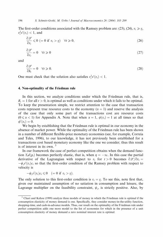
The first-order conditions associated with the Ramsey problem are: (23), (24), vt P v,v2t s
0ðvtÞ < 1, and
5 C
consum
shoppi
perfect
consum
oL
ovt6 0 ð¼ 0 if vt > vÞ 8tP 0; ð26Þ
oL
oct¼ 0 8tP 0 ð27Þ
and
oL
oht¼ 0 8tP 0: ð28Þ
One must check that the solution also satisfies v2t s0ðvtÞ < 1.
4. Non-optimality of the Friedman rule
In this section, we analyze conditions under which the Friedman rule, that is,
Rt ¼ 1 for all t > 0, is optimal as well as conditions under which it fails to be optimal.
To keep the presentation simple, we restrict attention to the case that transactioncosts represent true resource costs to the economy (a ¼ 1) and reserve the analysis
of the case that only some part of the transactions cost are resource costs
(06 a < 1) for Appendix A. Note that when a ¼ 1, /ðvtÞ ¼ 1 at all times so that
/0ðvtÞ ¼ 0.
We begin by establishing that the Friedman rule is optimal in our economy in the
absence of market power. While the optimality of the Friedman rule has been shown
in a number of different flexible-price monetary economies (see, for example, Correia
and Teles, 1996), to our knowledge, it has not previously been established for atransactions cost based monetary economy like the one we consider; thus this result
is of interest in its own. 5
In our framework the case of perfect competition obtains when the demand func-
tion YtdðptÞ becomes perfectly elastic, that is, when g ¼ �1. In this case the partial
derivative of the Lagrangian with respect to vt for t > 0 becomes oL=ovt ¼�wts
0ðvtÞct so that the first-order condition of the Ramsey problem with respect to
velocity is
�wts0ðvtÞct 6 0 ð¼ 0 if vt > vÞ:
The only solution to this first-order condition is vt ¼ v. To see this, note first that,
given our maintained assumption of no satiation in consumption and leisure, the
Lagrange multiplier on the feasibility constraint, wt, is strictly positive. Also, by
hari and Kehoe (1999) analyze three models of money in which the Friedman rule is optimal if the
ption elasticity of money demand is one. Specifically, they consider money-in-the-utility function,
ng-time, and cash-in-advance models. Thus, our result on the optimality of the Friedman rule under
competition adds one more model to the list of economies for which in the presence of a unit
ption elasticity of money demand a zero nominal interest rate is optimal.
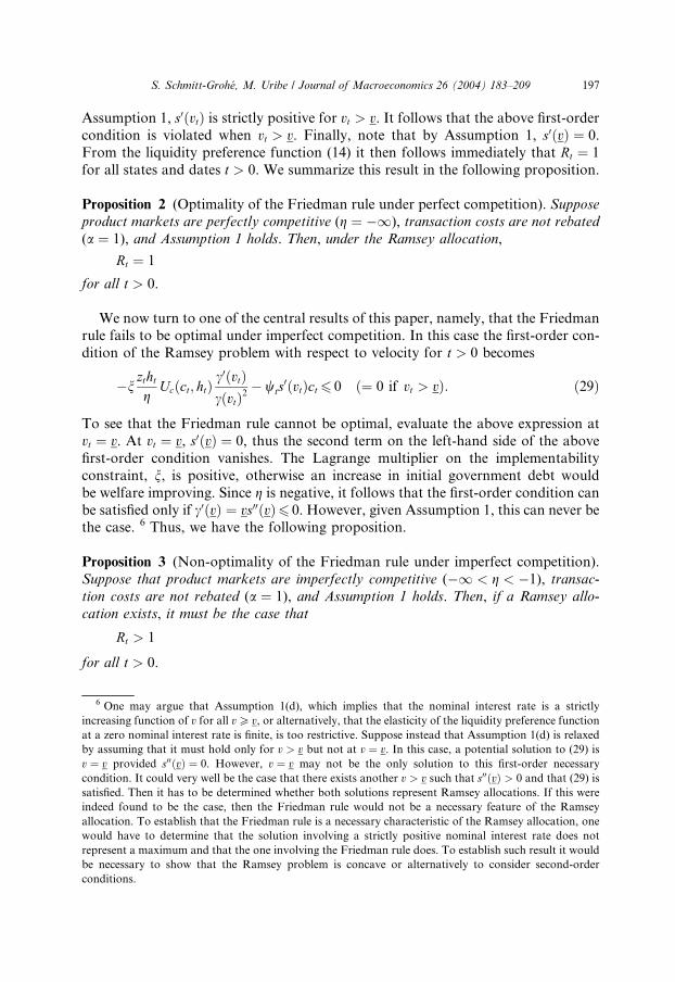
S. Schmitt-Groh�e, M. Uribe / Journal of Macroeconomics 26 (2004) 183–209 197
Assumption 1, s0ðvtÞ is strictly positive for vt > v. It follows that the above first-ordercondition is violated when vt > v. Finally, note that by Assumption 1, s0ðvÞ ¼ 0.
From the liquidity preference function (14) it then follows immediately that Rt ¼ 1
for all states and dates t > 0. We summarize this result in the following proposition.
Proposition 2 (Optimality of the Friedman rule under perfect competition). Supposeproduct markets are perfectly competitive (g ¼ �1), transaction costs are not rebated(a ¼ 1), and Assumption 1 holds. Then, under the Ramsey allocation,
6 O
increas
at a ze
by assu
v ¼ vcondit
satisfie
indeed
allocat
would
represe
be nec
condit
Rt ¼ 1
for all t > 0.
We now turn to one of the central results of this paper, namely, that the Friedman
rule fails to be optimal under imperfect competition. In this case the first-order con-
dition of the Ramsey problem with respect to velocity for t > 0 becomes
�nzthtg
Ucðct; htÞc0ðvtÞcðvtÞ2
� wts0ðvtÞct 6 0 ð¼ 0 if vt > vÞ: ð29Þ
To see that the Friedman rule cannot be optimal, evaluate the above expression at
vt ¼ v. At vt ¼ v, s0ðvÞ ¼ 0, thus the second term on the left-hand side of the above
first-order condition vanishes. The Lagrange multiplier on the implementability
constraint, n, is positive, otherwise an increase in initial government debt would
be welfare improving. Since g is negative, it follows that the first-order condition can
be satisfied only if c0ðvÞ ¼ vs00ðvÞ6 0. However, given Assumption 1, this can never bethe case. 6 Thus, we have the following proposition.
Proposition 3 (Non-optimality of the Friedman rule under imperfect competition).
Suppose that product markets are imperfectly competitive (�1 < g < �1), transac-tion costs are not rebated (a ¼ 1), and Assumption 1 holds. Then, if a Ramsey allo-cation exists, it must be the case that
Rt > 1
for all t > 0.
ne may argue that Assumption 1(d), which implies that the nominal interest rate is a strictly
ing function of v for all vP v, or alternatively, that the elasticity of the liquidity preference function
ro nominal interest rate is finite, is too restrictive. Suppose instead that Assumption 1(d) is relaxed
ming that it must hold only for v > v but not at v ¼ v. In this case, a potential solution to (29) is
provided s00ðvÞ ¼ 0. However, v ¼ v may not be the only solution to this first-order necessary
ion. It could very well be the case that there exists another v > v such that s00ðvÞ > 0 and that (29) is
d. Then it has to be determined whether both solutions represent Ramsey allocations. If this were
found to be the case, then the Friedman rule would not be a necessary feature of the Ramsey
ion. To establish that the Friedman rule is a necessary characteristic of the Ramsey allocation, one
have to determine that the solution involving a strictly positive nominal interest rate does not
nt a maximum and that the one involving the Friedman rule does. To establish such result it would
essary to show that the Ramsey problem is concave or alternatively to consider second-order
ions.
198 S. Schmitt-Groh�e, M. Uribe / Journal of Macroeconomics 26 (2004) 183–209
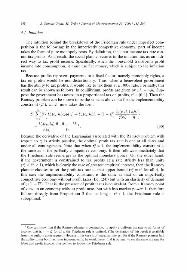
4.1. Intuition
The intuition behind the breakdown of the Friedman rule under imperfect com-
petition is the following: In the imperfectly competitive economy, part of income
takes the form of pure monopoly rents. By definition, the labor income tax rate can-not tax profits. As a result, the social planner resorts to the inflation tax as an indi-
rect way to tax profit income. Specifically, when the household transforms profit
income into consumption, it must use fiat money, which is subject to the inflation
tax.
Because profits represent payments to a fixed factor, namely monopoly rights, a
tax on profits would be non-distortionary. Thus, when a benevolent government
has the ability to tax profits, it would like to tax them at a 100% rate. Formally, this
result can be shown as follows. In equilibrium, profits are given by ztht � wtht. Sup-pose the government has access to a proportional tax on profits, spt 2 ½0; 1�. Then the
Ramsey problem can be shown to be the same as above but for the implementability
constraint (24), which now takes the form
7 O
incom
from t
the ab
labor a
E0
X1t¼0
bt Ucðct; htÞct/ðvtÞ�
þ Uhðct; htÞht þ ð1� spt ÞUcðct; htÞcðvtÞ
zthtg
�
¼ Ucðc0; h0Þcðv0Þ
R�1B�1 þM�1
P0: ð30Þ
Because the derivative of the Lagrangian associated with the Ramsey problem with
respect to spt is strictly positive, the optimal profit tax rate is one at all dates and
under all contingencies. Note that when spt ¼ 1, the implementability constraint is
the same as in the perfectly competitive economy. It then follows immediately that
the Friedman rule reemerges as the optimal monetary policy. On the other hand,
if the government is constrained to tax profits at a rate strictly less than unity
(spt < sp < 1), which is clearly the case of greatest empirical interest, then the Ramseyplanner chooses to set the profit tax rate at that upper bound (spt ¼ sp for all t). Inthis case the implementability constraint is the same as that of an imperfectly
competitive economy without profit taxes (Eq. (24)) but with an elasticity of demand
of g=ð1� spÞ. That is, the presence of profit taxes is equivalent, from a Ramsey point
of view, to an economy without profit taxes but with less market power. It therefore
follows directly from Proposition 3 that as long a sp < 1, the Friedman rule is
suboptimal. 7
ne can show that if the Ramsey planner is constrained to apply a uniform tax rate to all forms of
e, that is, st ¼ spt for all t, the Friedman rule is optimal. (The derivation of this result is available
he authors upon request.) However, this case is of marginal interest, for if the Ramsey planner had
ility to set both tax rates independently, he would never find it optimal to set the same tax rate for
nd profit income, thus neither to follow the Friedman rule.
S. Schmitt-Groh�e, M. Uribe / Journal of Macroeconomics 26 (2004) 183–209 199
5. Dynamic properties of Ramsey allocations
In this section we characterize numerically the dynamic properties of Ramsey
allocations. We begin by proposing a solution method that does not rely on any type
of approximation of the non-linear Ramsey conditions. Then we describe the cali-bration of the model. Finally, we present the quantitative results.
5.1. Solution method
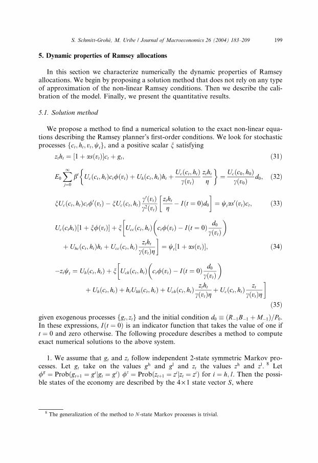
We propose a method to find a numerical solution to the exact non-linear equa-
tions describing the Ramsey planner’s first-order conditions. We look for stochastic
processes fct; ht; vt;wtg, and a positive scalar n satisfying
8 Th
ztht ¼ ½1þ asðvtÞ�ct þ gt; ð31Þ
E0
X1j¼0
bt Ucðct; htÞct/ðvtÞ�
þ Uhðct; htÞht þUcðct; htÞcðvtÞ
zthtg
�¼ Ucðc0; h0Þ
cðv0Þd0; ð32Þ
nUcðct; htÞct/0ðvtÞ � nUcðct; htÞc0ðvtÞc2ðvtÞ
zthtg
�� Iðt ¼ 0Þd0
�¼ wtas
0ðvtÞct; ð33Þ
UcðcthtÞ½1þ n/ðvtÞ� þ n Uccðct; htÞ ct/ðvtÞ��
� Iðt ¼ 0Þ d0cðvtÞ
�
þ Uhcðct; htÞht þ Uccðct; htÞztht
cðvtÞg
�¼ wt½1þ asðvtÞ�; ð34Þ
�ztwt ¼ Uhðct; htÞ þ n Uchðct; htÞ ct/ðvtÞ��
� Iðt ¼ 0Þ d0cðvtÞ
�
þ Uhðct; htÞ þ htUhhðct; htÞ þ Uchðct; htÞztht
cðvtÞgþ Ucðct; htÞ
ztcðvtÞg
�
ð35Þ
given exogenous processes fgt; ztg and the initial condition d0 � ðR�1B�1 þM�1Þ=P0.In these expressions, Iðt ¼ 0Þ is an indicator function that takes the value of one if
t ¼ 0 and zero otherwise. The following procedure describes a method to compute
exact numerical solutions to the above system.
1. We assume that gt and zt follow independent 2-state symmetric Markov pro-cesses. Let gt take on the values gh and gl and zt the values zh and zl. 8 Let
/g ¼ Probðgtþ1 ¼ gijgt ¼ giÞ /z ¼ Probðztþ1 ¼ zijzt ¼ ziÞ for i ¼ h; l. Then the possi-
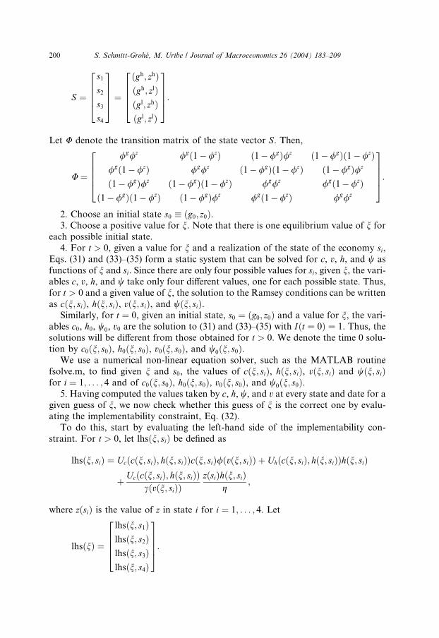
ble states of the economy are described by the 4 · 1 state vector S, where
e generalization of the method to N -state Markov processes is trivial.
200 S. Schmitt-Groh�e, M. Uribe / Journal of Macroeconomics 26 (2004) 183–209
S ¼
s1s2s3s4
26664
37775 ¼
ðgh; zhÞðgh; zlÞðgl; zhÞðgl; zlÞ
26664
37775:
Let U denote the transition matrix of the state vector S. Then,
U¼
/g/z /gð1�/zÞ ð1�/gÞ/z ð1�/gÞð1�/zÞ/gð1�/zÞ /g/z ð1�/gÞð1�/zÞ ð1�/gÞ/z
ð1�/gÞ/z ð1�/gÞð1�/zÞ /g/z /gð1�/zÞð1�/gÞð1�/zÞ ð1�/gÞ/z /gð1�/zÞ /g/z
26664
37775:
2. Choose an initial state s0 � ðg0; z0Þ.3. Choose a positive value for n. Note that there is one equilibrium value of n for
each possible initial state.
4. For t > 0, given a value for n and a realization of the state of the economy si,Eqs. (31) and (33)–(35) form a static system that can be solved for c, v, h, and w as
functions of n and si. Since there are only four possible values for si, given n, the vari-ables c, v, h, and w take only four different values, one for each possible state. Thus,
for t > 0 and a given value of n, the solution to the Ramsey conditions can be written
as cðn; siÞ, hðn; siÞ, vðn; siÞ, and wðn; siÞ.Similarly, for t ¼ 0, given an initial state, s0 ¼ ðg0; z0Þ and a value for n, the vari-
ables c0, h0, w0, v0 are the solution to (31) and (33)–(35) with Iðt ¼ 0Þ ¼ 1. Thus, the
solutions will be different from those obtained for t > 0. We denote the time 0 solu-
tion by c0ðn; s0Þ, h0ðn; s0Þ, v0ðn; s0Þ, and w0ðn; s0Þ.We use a numerical non-linear equation solver, such as the MATLAB routine
fsolve.m, to find given n and s0, the values of cðn; siÞ, hðn; siÞ, vðn; siÞ and wðn; siÞfor i ¼ 1; . . . ; 4 and of c0ðn; s0Þ, h0ðn; s0Þ, v0ðn; s0Þ, and w0ðn; s0Þ.
5. Having computed the values taken by c, h, w, and v at every state and date for agiven guess of n, we now check whether this guess of n is the correct one by evalu-
ating the implementability constraint, Eq. (32).
To do this, start by evaluating the left-hand side of the implementability con-
straint. For t > 0, let lhsðn; siÞ be defined as
lhsðn; siÞ ¼ Ucðcðn; siÞ; hðn; siÞÞcðn; siÞ/ðvðn; siÞÞ þ Uhðcðn; siÞ; hðn; siÞÞhðn; siÞ
þ Ucðcðn; siÞ; hðn; siÞÞcðvðn; siÞÞ
zðsiÞhðn; siÞg
;
where zðsiÞ is the value of z in state i for i ¼ 1; . . . ; 4. Let
lhsðnÞ ¼
lhsðn; s1Þlhsðn; s2Þlhsðn; s3Þlhsðn; s4Þ
26664
37775:
S. Schmitt-Groh�e, M. Uribe / Journal of Macroeconomics 26 (2004) 183–209 201
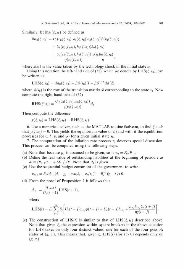
Similarly, let lhs0ðn; s0Þ be defined as
lhs0ðn; s0Þ ¼ Ucðc0ðn; s0Þ; h0ðn; s0ÞÞc0ðn; s0Þ/ðv0ðn; s0ÞÞ
þ Uhðc0ðn; s0Þ; h0ðn; s0ÞÞh0ðn; s0Þ
þ Ucðc0ðn; s0Þ; h0ðn; s0ÞÞcðv0ðn; s0ÞÞ
zðs0Þh0ðn; s0Þg
;
where zðs0Þ is the value taken by the technology shock in the initial state s0.Using this notation the left-hand side of (32), which we denote by LHSðn; s0Þ, can
be written as
LHSðn; s0Þ ¼ lhs0ðn; s0Þ þ bUðs0ÞðI � bUÞ�1lhsðnÞ;
where Uðs0Þ is the row of the transition matrix U corresponding to the state s0. Now
compute the right-hand side of (32)
RHSðn; s0Þ ¼Ucðc0ðn; s0Þ; h0ðn; s0ÞÞ
cðv0ðn; s0ÞÞd0:
Then compute the difference
yðn; s0Þ ¼ LHSðn; s0Þ �RHSðn; s0Þ:
6. Use a numerical solver, such as the MATLAB routine fsolve.m, to find n suchthat yðn; s0Þ ¼ 0. This yields the equilibrium value of n (and with it the equilibrium
processes for c, h, v, and w) for a given initial state s0.7. The computation of the inflation rate process pt deserves special discussion.
This process can be computed using the following steps.
(a) Note that because p0 is assumed to be given, so is p0 ¼ P0=P�1.
(b) Define the real value of outstanding liabilities at the beginning of period t asdt � ðRt�1Bt�1 þMt�1Þ=Pt. Note that d0 is given.
(c) Use the sequential budget constraint of the government to write
ptþ1 ¼ Rt=dtþ1½dt þ gt � stwtht � ct=vtð1� R�1t Þ�; tP 0:
(d) From the proof of Proposition 1 it follows that
dtþ1 ¼cðvtþ1Þ
Ucðt þ 1ÞLHSðt þ 1Þ;
where
LHSðtÞ ¼ Et
X1j¼0
bj Ucðt�
þ jÞctþj/ðt þ jÞ þ Uhðt þ jÞhtþj þztþjhtþjUcðt þ jÞ
gcðt þ jÞ
�:
(e) The construction of LHSðtÞ is similar to that of LHSðn; s0Þ described above.
Note that given n, the expression within square brackets in the above equationfor LHS takes on only four distinct values, one for each of the four possible
states of ðgt; ztÞ. This means that, given n, LHSðtÞ (for t > 0) depends only on
ðgt; ztÞ.
202 S. Schmitt-Groh�e, M. Uribe / Journal of Macroeconomics 26 (2004) 183–209
We now put this method to work by computing the dynamic properties of the
Ramsey allocation in a simple calibrated economy.
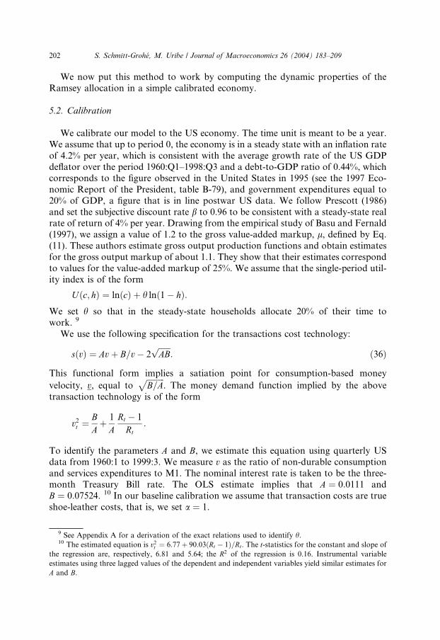
5.2. Calibration
We calibrate our model to the US economy. The time unit is meant to be a year.
We assume that up to period 0, the economy is in a steady state with an inflation rate
of 4.2% per year, which is consistent with the average growth rate of the US GDP
deflator over the period 1960:Q1–1998:Q3 and a debt-to-GDP ratio of 0.44%, which
corresponds to the figure observed in the United States in 1995 (see the 1997 Eco-
nomic Report of the President, table B-79), and government expenditures equal to
20% of GDP, a figure that is in line postwar US data. We follow Prescott (1986)
and set the subjective discount rate b to 0.96 to be consistent with a steady-state realrate of return of 4% per year. Drawing from the empirical study of Basu and Fernald
(1997), we assign a value of 1.2 to the gross value-added markup, l, defined by Eq.
(11). These authors estimate gross output production functions and obtain estimates
for the gross output markup of about 1.1. They show that their estimates correspond
to values for the value-added markup of 25%. We assume that the single-period util-
ity index is of the form
9 Se10 T
the reg
estima
A and
Uðc; hÞ ¼ lnðcÞ þ h lnð1� hÞ:
We set h so that in the steady-state households allocate 20% of their time towork. 9
We use the following specification for the transactions cost technology:
sðvÞ ¼ Avþ B=v� 2ffiffiffiffiffiffiAB
p: ð36Þ
This functional form implies a satiation point for consumption-based money
velocity, v, equal toffiffiffiffiffiffiffiffiffiB=A
p. The money demand function implied by the above
transaction technology is of the form
v2t ¼BAþ 1
ARt � 1
Rt:
To identify the parameters A and B, we estimate this equation using quarterly US
data from 1960:1 to 1999:3. We measure v as the ratio of non-durable consumption
and services expenditures to M1. The nominal interest rate is taken to be the three-
month Treasury Bill rate. The OLS estimate implies that A ¼ 0:0111 and
B ¼ 0:07524. 10 In our baseline calibration we assume that transaction costs are true
shoe-leather costs, that is, we set a ¼ 1.
e Appendix A for a derivation of the exact relations used to identify h.he estimated equation is v2t ¼ 6:77þ 90:03ðRt � 1Þ=Rt. The t-statistics for the constant and slope of
ression are, respectively, 6.81 and 5.64; the R2 of the regression is 0.16. Instrumental variable
tes using three lagged values of the dependent and independent variables yield similar estimates for
B.
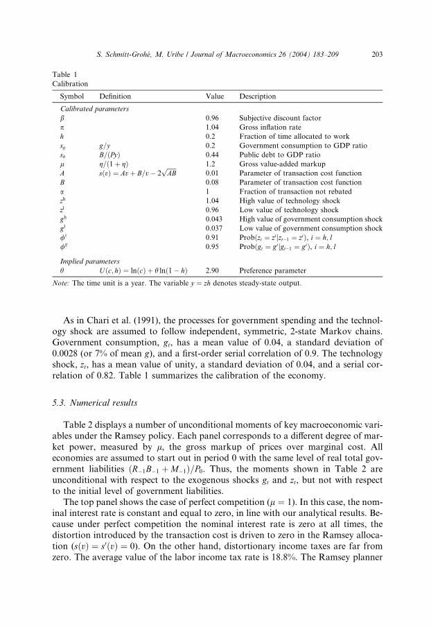
Table 1
Calibration
Symbol Definition Value Description
Calibrated parameters
b 0.96 Subjective discount factor
p 1.04 Gross inflation rate
h 0.2 Fraction of time allocated to work
sg g=y 0.2 Government consumption to GDP ratio
sb B=ðPyÞ 0.44 Public debt to GDP ratio
l g=ð1þ gÞ 1.2 Gross value-added markup
A sðvÞ ¼ Avþ B=v� 2ffiffiffiffiffiffiAB
p0.01 Parameter of transaction cost function
B 0.08 Parameter of transaction cost function
a 1 Fraction of transaction not rebated
zh 1.04 High value of technology shock
zl 0.96 Low value of technology shock
gh 0.043 High value of government consumption shock
gl 0.037 Low value of government consumption shock
/z 0.91 Probðzt ¼ zijzt�1 ¼ ziÞ, i ¼ h; l/g 0.95 Probðgt ¼ gijgt�1 ¼ giÞ, i ¼ h; l
Implied parameters
h Uðc; hÞ ¼ lnðcÞ þ h lnð1� hÞ 2.90 Preference parameter
Note: The time unit is a year. The variable y ¼ zh denotes steady-state output.
S. Schmitt-Groh�e, M. Uribe / Journal of Macroeconomics 26 (2004) 183–209 203
As in Chari et al. (1991), the processes for government spending and the technol-ogy shock are assumed to follow independent, symmetric, 2-state Markov chains.
Government consumption, gt, has a mean value of 0.04, a standard deviation of
0.0028 (or 7% of mean g), and a first-order serial correlation of 0.9. The technology
shock, zt, has a mean value of unity, a standard deviation of 0.04, and a serial cor-
relation of 0.82. Table 1 summarizes the calibration of the economy.
5.3. Numerical results
Table 2 displays a number of unconditional moments of key macroeconomic vari-
ables under the Ramsey policy. Each panel corresponds to a different degree of mar-
ket power, measured by l, the gross markup of prices over marginal cost. All
economies are assumed to start out in period 0 with the same level of real total gov-
ernment liabilities ðR�1B�1 þM�1Þ=P0. Thus, the moments shown in Table 2 are
unconditional with respect to the exogenous shocks gt and zt, but not with respect
to the initial level of government liabilities.
The top panel shows the case of perfect competition (l ¼ 1). In this case, the nom-inal interest rate is constant and equal to zero, in line with our analytical results. Be-
cause under perfect competition the nominal interest rate is zero at all times, the
distortion introduced by the transaction cost is driven to zero in the Ramsey alloca-
tion (sðvÞ ¼ s0ðvÞ ¼ 0). On the other hand, distortionary income taxes are far from
zero. The average value of the labor income tax rate is 18.8%. The Ramsey planner
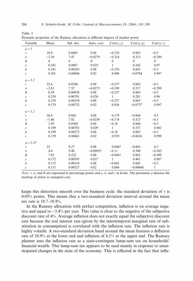
Table 2
Dynamic properties of the Ramsey allocation at different degrees of market power
Variable Mean Std. dev. Auto. corr. Corrðx; yÞ Corrðx; gÞ Corrðx; zÞl¼ 1
s 18.8 0.0491 0.88 )0.276 0.865 )0.5p )3.39 7.47 )0.0279 )0.214 0.315 )0.299R 0 0 0 0 0 0
y 0.241 0.0087 0.825 1 0.242 0.97
h 0.241 0.00243 0.88 )0.276 0.865 )0.5c 0.201 0.00846 0.82 0.948 )0.0784 0.997
l¼ 1.1
s 22.6 0.0296 0.88 )0.237 0.865 )0.5p )2.81 7.52 )0.0273 )0.199 0.317 )0.299R 0.59 0.00938 0.88 )0.237 0.865 )0.5y 0.219 0.00781 0.826 1 0.281 0.96
h 0.219 0.00254 0.88 )0.237 0.865 )0.5c 0.179 0.00752 0.82 0.936 )0.0757 0.997
l¼ 1.2
s 26.6 0.042 0.88 0.179 )0.864 0.5
p )1.46 7.92 )0.0239 )0.174 0.323 )0.3R 1.95 0.0369 0.88 )0.18 0.864 )0.5y 0.199 0.00701 0.829 1 0.337 0.942
h 0.199 0.00273 0.88 )0.18 0.865 )0.5c 0.159 0.00661 0.82 0.919 )0.0616 0.998
l¼ 1.35
s 33 0.27 0.88 0.0447 )0.865 0.5
p 4.4 9.48 )0.00953 )0.11 0.349 )0.305R 7.83 0.222 0.88 )0.0447 0.862 )0.499y 0.172 0.00595 0.837 1 0.461 0.887
h 0.172 0.00318 0.88 )0.045 0.865 )0.5c 0.131 0.00527 0.82 0.884 )0.00668 1
Note: s, p, and R are expressed in percentage points and y, h, and c in levels. The parameter l denotes the
markup of prices to marginal cost.
204 S. Schmitt-Groh�e, M. Uribe / Journal of Macroeconomics 26 (2004) 183–209
keeps this distortion smooth over the business cycle; the standard deviation of s is0.05% points. This means that a two-standard deviation interval around the mean
tax rate is 18.7–18.9%.
In the Ramsey allocation with perfect competition, inflation is on average nega-
tive and equal to )3.4% per year. This value is close to the negative of the subjective
discount rate of 4%. Average inflation does not exactly equal the subjective discount
rate because the real interest rate (given by the intertemporal marginal rate of sub-
stitution in consumption) is correlated with the inflation rate. The inflation rate is
highly volatile. A two-standard deviation band around the mean features a deflationrate of 10.9% at the lower end and inflation of 4.1% at the upper end. The Ramsey
planner uses the inflation rate as a state-contingent lump-sum tax on households’
financial wealth. This lump-sum tax appears to be used mainly in response to unan-
ticipated changes in the state of the economy. This is reflected in the fact that infla-
S. Schmitt-Groh�e, M. Uribe / Journal of Macroeconomics 26 (2004) 183–209 205
tion displays a near zero serial correlation. 11 The high volatility and low persistence
of the inflation rate stands in sharp contrast to the smooth and highly persistent
behavior of the labor income tax rate. Our results on the dynamic properties of
the Ramsey economy under perfect competition are consistent with those obtained
by Chari et al. (1991). 12
As soon as one moves away from the assumption of perfect competition, the
Friedman rule ceases to be optimal. A central result of Table 2 is that the average
optimal nominal interest rate is an increasing function of the profit share, which
in our economy is related to the markup by the function ðl� 1Þ=l. 13 As the markup
increases from 1 to 1.35, or the profit share increases from 0% to 25%, the average
nominal interest rate increases from 0% to 7.8% per year.
Because when the interest rate increases so do interest savings from the issuance of
money, one might be led to believe that as the markup increases the governmentmight lower income tax rates to compensate for the increase in seignorage revenue.
However, as Table 2 shows, this is not the case here. The average labor income tax
rate increases sharply from 18.8% to 33.3% as the markup rises from 0% to 35%. The
reason for the Ramsey planner’s need to increase tax rates when the markup goes up
is that the labor income tax base falls as both employment and wages fall as the econ-
omy becomes less competitive. Indeed employment falls from 0.24 to 0.17 and wages
fall from 1 to 0.74 as l increases from 1 to 1.35.
Another result that emerges from inspection of Table 2 is that, unlike under per-fect competition, in the presence of market power the Ramsey planner chooses not to
keep the nominal interest rate constant along the business cycle. Although small, the
volatility of the nominal interest rate increases with the markup. The standard devi-
ation of the nominal interest rate increases to 22 basis points as the degree of market
power increases from 0% to 35%. In addition, the nominal interest rate is highly per-
sistent, with a serial correlation of 0.88, highly correlated with government pur-
chases, with a correlation coefficient of 0.86, and negatively correlated with the
technology shock, with a correlation of )0.5.
11 The observation that in the Ramsey equilibrium inflation acts as a lump-sum tax on wealth was, to
our knowledge, first made by Chari et al. (1991) and has recently been stressed by Sims (2001).12 The main quantitative difference in results is that Chari et al. find a standard deviation of inflation of
19.93% points which is more than twice the value we report in Table 2. The source of this discrepancy may
lie in the fact that Chari et al. use a different solution method. One might think that the disparity could be
due to the fact that the models incorporate different motivations for the demand for money. We assume
that money reduces transactions costs, whereas Chari et al. use a cash–credit goods model. However, since
in both frameworks the Friedman rule is optimal, the monetary distortion vanishes in both setups and thus
should not play any role for the properties of the Ramsey allocation. Of course, the two models might
imply different values for the average ratio of money to GDP. Since money is one component of
households’ financial wealth, which in turn is the tax base of the state-contingent lump-sum tax embodied
in inflation, the different money demand specifications may in principle explain the difference in the
volatility of inflation. However, we experimented using the steady-state money-to-GDP and the debt-to-
GDP ratios used by Chari et al. and found that the volatility of inflation is not significantly different from
the value we report in Table 2.13 Profits and monopoly power need not be related in this way. For instance, in the presence of fixed
costs the average profit share can be significantly smaller than ðl� 1Þ=l.
206 S. Schmitt-Groh�e, M. Uribe / Journal of Macroeconomics 26 (2004) 183–209
Finally as in the case of perfect competition, tax rates are little volatile and per-
sistent and inflation is highly volatile and almost serially uncorrelated.
6. Summary and conclusion
In this paper we have characterized optimal fiscal and monetary policy in an econ-
omy with market power in product markets. The study was conducted within a stan-
dard stochastic, dynamic, monetary economy with production but no capital. The
production technology is assumed to be subject to exogenous stochastic productivity
shocks. The government finances an exogenous and stochastic stream of government
purchases by issuing money, levying distortionary income taxes, and issuing bonds.
Public debt takes the form of nominal, non-state-contingent government obligations.In this economy, under perfect competition the Friedman rule is optimal. The cen-
tral result of this paper is that once pure profits are introduced through imperfect
competition, the Friedman rule ceases to be optimal. Indeed, the nominal interest
rate increases with the profit share. In addition, in the presence of pure monopoly
rents, the optimal nominal interest rate is time varying and its unconditional volatil-
ity increases with the magnitude of such rents.
A number of important properties of the Ramsey allocation under perfect compe-
tition are, however, robust to the introduction of market power. In particular,regardless of the degree of monopoly power the income tax rate displays very little
volatility and is highly persistent. By contrast, the inflation rate is highly volatile and
nearly serially uncorrelated. This shows that as in the case of perfect competition,
under monopoly power the government uses the inflation rate as a state-contingent,
lump-sum tax on total financial wealth. This lump-sum tax allows the government to
refrain from changing distortionary taxes in response to adverse government pur-
chases or productivity shocks.
In conducting the analysis of optimal fiscal and monetary policy we restricted atten-tion to a specific motivation for the demand for money. Namely, one in which money
reduces transaction costs associated with purchases of final goods.We conjecture, how-
ever, that our central result regarding the breakdown of the Friedman rule in the pres-
ence of imperfect competition holds in any monetary model where inflation acts as a
tax on income or consumption. This is the case because as long as profit tax rates
are bounded away from 100%, which is arguably the most realistic case, a benevolent
government will have an incentive to use inflation as an indirect way to tax profits.
This paper can be extended in several directions. A natural one, which we persuein Schmitt-Groh�e and Uribe (in press), is to introduce nominal rigidities in the form
of sticky prices. One motivation for considering such an extension is that under price
flexibility the Ramsey allocation calls for highly volatile inflation rates. This aspect
of the optimal policy regime is at odds with conventional wisdom about the desir-
ability of price stability. Sticky prices may contribute to bringing down the optimal
degree of inflation volatility. In Schmitt-Groh�e and Uribe (in press), we show that
the incorporation of sticky prices into a model like the one analyzed in this paper
introduces a significant modification in the primal form of the Ramsey problem. Spe-
S. Schmitt-Groh�e, M. Uribe / Journal of Macroeconomics 26 (2004) 183–209 207
cifically, under sticky prices and non-state-contingent nominal government debt, it is
no longer the case that the implementability constraint takes the form of a single in-
tertemporal restriction. Instead, it is replaced by a sequence of constraints like (24),
one for each date and state of the world. This modification of the Ramsey problem is
similar to the one that takes place in real models in which real public debt is re-stricted to be non-state-contingent like the one studied by Aiyagari et al. (2002).
More broadly, because imperfect competition is an essential element of modern
general equilibrium formulations of sticky-price models, the present study can be
viewed as an intermediate step in the quest for understanding the properties of opti-
mal fiscal and monetary policy in models with sluggish nominal price adjustment.
Acknowledgements
We would like to thank Chuck Carlstrom and Harald Uhlig for comments.
Appendix A
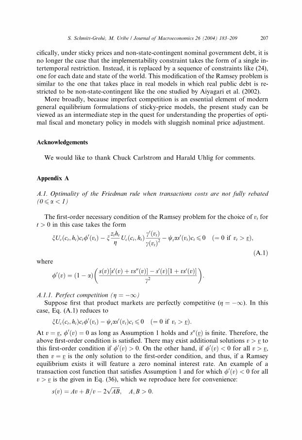
A.1. Optimality of the Friedman rule when transactions costs are not fully rebated
(06 a < 1)
The first-order necessary condition of the Ramsey problem for the choice of vt fort > 0 in this case takes the form
nUcðct; htÞct/0ðvtÞ � nzthtg
Ucðct; htÞc0ðvtÞcðvtÞ2
� wtas0ðvtÞct 6 0 ð¼ 0 if vt > vÞ;
ðA:1Þ
where/0ðvÞ ¼ ð1� aÞ sðvÞ½s0ðvÞ þ vs00ðvÞ� � s0ðvÞ½1þ vs0ðvÞ�c2
� �:
A.1.1. Perfect competition (g ¼ �1)
Suppose first that product markets are perfectly competitive (g ¼ �1). In this
case, Eq. (A.1) reduces to
nUcðct; htÞct/0ðvtÞ � wtas0ðvtÞct 6 0 ð¼ 0 if vt > vÞ:
At v ¼ v, /0ðvÞ ¼ 0 as long as Assumption 1 holds and s00ðvÞ is finite. Therefore, theabove first-order condition is satisfied. There may exist additional solutions v > v tothis first-order condition if /0ðvÞ > 0. On the other hand, if /0ðvÞ < 0 for all v > v,then v ¼ v is the only solution to the first-order condition, and thus, if a Ramsey
equilibrium exists it will feature a zero nominal interest rate. An example of a
transaction cost function that satisfies Assumption 1 and for which /0ðvÞ < 0 for all
v > v is the given in Eq. (36), which we reproduce here for convenience:
sðvÞ ¼ Avþ B=v� 2ffiffiffiffiffiffiAB
p; A;B > 0:
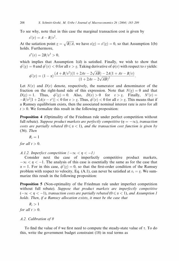
208 S. Schmitt-Groh�e, M. Uribe / Journal of Macroeconomics 26 (2004) 183–209
To see why, note that in this case the marginal transaction cost is given by
s0ðvÞ ¼ A� B=v2:
At the satiation point v ¼ffiffiffiffiffiffiffiffiffiB=A
p; we have sðvÞ ¼ s0ðvÞ ¼ 0, so that Assumption 1(b)
holds. Furthermore,
s00ðvÞ ¼ 2B=v3 > 0;
which implies that Assumption 1(d) is satisfied. Finally, we wish to show that
/0ðvÞ ¼ 0 and /0ðvÞ < 0 for all v > v. Taking derivative of /ðvÞwith respect to v yields:
/0ðvÞ ¼ ð1� aÞ ðAþ B=v2Þð1þ 2Av� 2ffiffiffiffiffiffiAB
pÞ � 2Að1þ Av� B=vÞ
ð1þ 2Av� 2ffiffiffiffiffiffiAB
pÞ2
:
Let NðvÞ and DðvÞ denote, respectively, the numerator and denominator of the
fraction on the right-hand side of this expression. Note that NðvÞ ¼ 0 and thatDðvÞ ¼ 1. Thus, /0ðvÞ ¼ 0. Also, DðvÞ > 0 for v > v. Finally, N 0ðvÞ ¼�B=v2½1þ 2Aðv� vsÞ� < 0 for v > v. Thus, /0ðvÞ < 0 for all v > v. This means that if
a Ramsey equilibrium exists, then the associated nominal interest rate is zero for all
t > 0. We formalize this result in the following proposition:
Proposition 4 (Optimality of the Friedman rule under perfect competition without
full rebate). Suppose product markets are perfectly competitive (g ¼ �1), transactioncosts are partially rebated (06 a < 1), and the transaction cost function is given by(36). Then
Rt ¼ 1
for all t > 0.
A.1.2. Imperfect competition (�1 < g < �1)
Consider next the case of imperfectly competitive product markets,
�1 < g < �1. The analysis of this case is essentially the same as for the case that
a ¼ 1. For in this case, /0ðvÞ ¼ 0, so that the first-order condition of the Ramsey
problem with respect to velocity, Eq. (A.1), can never be satisfied at vt ¼ v. We sum-
marize this result in the following proposition:
Proposition 5 (Non-optimality of the Friedman rule under imperfect competition
without full rebate). Suppose that product markets are imperfectly competitive(�1 < g < �1), transaction costs are partially rebated (06 a < 1), and Assumption 1
holds. Then, if a Ramsey allocation exists, it must be the case that
Rt > 1
for all t > 0.
A.2. Calibration of h
To find the value of h we first need to compute the steady-state value of s. To do
this, write the government budget constraint (18) in real terms as
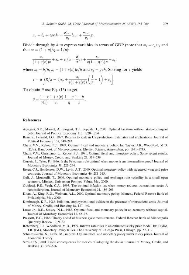
S. Schmitt-Groh�e, M. Uribe / Journal of Macroeconomics 26 (2004) 183–209 209
mt þ bt þ stwtht ¼Rt�1
ptbt�1 þ
mt�1
ptgt:
Divide through by h to express variables in terms of GDP (note that mt ¼ ct=vt andthat w ¼ ð1þ gÞ=g ¼ 1=l):
scð1þ sðvÞÞvþ sb þ st=l ¼ R
psb þ
scvð1þ sðvÞÞpþ sg;
where sb ¼ b=h, sc ¼ ð1þ sðvÞÞc=h and sg ¼ g=h. Solving for s yields
s ¼ l ðR=p�
� 1Þsb þsc
vð1þ sðvÞÞ1
p
�� 1
�þ sg
�:
To obtain h use Eq. (13) to get
h ¼ 1� scðvÞ
1þ sðvÞsc
1þ gg
1� hh
:
References
Aiyagari, S.R., Marcet, A., Sargent, T.J., Sepp€al€a, J., 2002. Optimal taxation without state-contingent
debt. Journal of Political Economy 110, 1220–1254.
Basu, S., Fernald, J.G., 1997. Returns to scale in US production: Estimates and implications. Journal of
Political Economy 105, 249–283.
Chari, V.V., Kehoe, P.J., 1999. Optimal fiscal and monetary policy. In: Taylor, J.B., Woodford, M.D.
(Eds.), Handbook of Macroeconomics. Elsevier Science, Amsterdam, pp. 1671–1745.
Chari, V.V., Christiano, L., Kehoe, P.J., 1991. Optimal fiscal and monetary policy: Some recent results.
Journal of Money, Credit, and Banking 23, 519–539.
Correia, I., Teles, P., 1996. Is the Friedman rule optimal when money is an intermediate good? Journal of
Monetary Economics 38, 223–244.
Erceg, C.J., Henderson, D.W., Levin, A.T., 2000. Optimal monetary policy with staggered wage and price
contracts. Journal of Monetary Economics 46, 281–313.
Gal�ı, J., Monacelli, T., 2000. Optimal monetary policy and exchange rate volatility in a small open
economy, Mimeo., Universitat Pompeu Fabra, May 2000.
Guidotti, P.E., V�egh, C.A., 1993. The optimal inflation tax when money reduces transactions costs: A
reconsideration. Journal of Monetary Economics 31, 189–205.
Khan, A., King, R.G., Wolman, A.L., 2000. Optimal monetary policy, Mimeo., Federal Reserve Bank of
Philadelphia, May 2000.
Kimbrough, K.P., 1986. Inflation, employment, and welfare in the presence of transactions costs. Journal
of Money, Credit, and Banking 18, 127–140.
Lucas Jr., R.E., Stokey, N.L., 1983. Optimal fiscal and monetary policy in an economy without capital.
Journal of Monetary Economics 12, 55–93.
Prescott, E.C., 1986. Theory ahead of business cycle measurement. Federal Reserve Bank of Minneapolis
Quarterly Review 10, 9–22.
Rotemberg, J.J., Woodford, M.D., 1999. Interest rate rules in an estimated sticky price model. In: Taylor,
J.B. (Ed.), Monetary Policy Rules. The University of Chicago Press, Chicago, pp. 57–119.
Schmitt-Groh�e, S., Uribe, M., in press. Optimal fiscal and monetary policy under sticky prices. Journal of
Economic Theory.
Sims, C.A., 2001. Fiscal consequences for mexico of adopting the dollar. Journal of Money, Credit, and
Banking 33, 597–616.