1

Optimal Scheduling of Battery Charging StationServing Electric Vehicles Based on Battery Swapping

Xiaoqi Tan, Guannan Qu, Bo Sun, Na Li, and Danny H.K. Tsang

Abstract—A battery charging station (BCS) is a chargingfacility that supplies electric energy for recharging electricvehicles’ depleted batteries (DBs). A BCS has a certain numberof charging bays and maintains a dynamic inventory of fully-charged batteries (FBs). This paper studies a BCS schedul-ing (BCSS) problem whose target is to schedule the chargingprocesses of the charging bays such that the charging cost isminimized while satisfying the FB demand. Specifically, the BCSSproblem has two types of operations: i) loading DBs into thecharging bays and then unloading them to the FB inventorywhen they are fully-charged, and ii) controlling the chargingrate of each charging bay. We formulate the BCSS problemas a mixed-integer program with quadratic battery degradationcost. A generalized Benders decomposition algorithm is thendeveloped to solve the problem efficiently. The salience of thedeveloped algorithm is that i) each charging bay can solve itsown subproblem separately, and ii) each subproblem can befurther partitioned into multiple simple quadratic programmingproblems, and thus the algorithm facilitates an efficient parallelimplementation. We perform extensive real data simulation tovalidate the optimization model and demonstrate the efficiencyof the proposed algorithm.

Index Terms—Battery Charging Station, Charging Scheduling,Electric Vehicles, Generalized Benders Decomposition, BatterySwapping

NOMENCLATURE

AcronymsBCS Battery Charging StationBCSS Battery Charging Station SchedulingBDC Battery Degradation CostBSS Battery Swapping StationCB Charging BayDB Depleted BatteryEPC Electricity Purchasing CostFB Fully-Charged BatterySoC State-of-Charge of batteriesIndices and Parametersα The minimum level of SoC for a battery to be

regarded as fully-charged.∆T The length of each time slot.ηb Charging efficiency of the b-th CB.B Set of all CBs.Gb(·) The battery degradaction cost function.T Set of time slots {0, · · · , T − 1}.CBb The b-th CB.θ The capacity of batteries.B Total number of charging bays.

X. Tan, B. Sun, and D.H.K. Tsang are with the Department of Electronicand Computer Engineering, Hong Kong University of Science and Technol-ogy, Hong Kong (E-mail: {xtanaa, bsunaa, eetsang}@ust.hk). Guannan Quand Na Li are with the School of Engineering and Applied Science, HarvardUniversity (E-mail: gqu@g.harvard.edu, lina@seas.harvard.edu).

b Index for CBs.C Transmission line capacitydt FB demand at time tFt Total number of FBs at time t.Lt Non-battery load at time slot tpt Electricity price at time slot t.rmaxb Maximum charging rate of CBb.sb,t SoC of the battery in CBb at time t.snewb,t SoC of the newly-loaded battery in CBb at t.sinitialb Initial SoC of battery in CBb.T Total number of time slots.Decision Variablesrb,t Continuous decision variable: charging rate of the

battery in CBb at time slot t.ub,t Binary decision variable: ‘1’ if the battery in CBb

at time t is unloaded; ‘0’ otherwise.

I. INTRODUCTION

As the adoption rate of electric vehicles (EVs) is increasing,there is a growing demand for fast and convenient energyrefueling services. Currently, EV energy refueling is mainlyperformed by several well-known charging methods, such asslow charging at home [1] and fast charging at public chargingstations [2]. However, many EVs, especially electric buses andtaxis, have started to support swappable batteries [3], [4], andthis facilitates an alternative EV energy refueling method, i.e.,the battery-swapping method [5], [6].

Compared to the long charging time of existing chargingmethods (usually in hours), with the battery-swapping methodan EV can swap its depleted battery (DB) for a fully-chargedbattery (FB) one at a battery swapping station (BSS) withinseveral minutes [3], or even in tens of seconds [6]. Theswapped DBs from different BSSs can be gathered togetherand recharged at a centralized battery charging station (BCS),which thus forms a gigantic battery energy storage system.It is believed that if appropriately planned and managed, thebattery-swapping technology can not only benefit EV ownerswith a fast energy refueling service [7], but it can also provideenormous flexibility for grid operators to perform critical taskssuch as load balancing [8] and renewable energy integration[9], [10], thus reducing carbon emissions [11] and improvingthe efficiency and stability of power systems [12].

A. Related Work

Undoubtedly, successful implementation of an EV energyrefueling system based on battery swapping necessitates awell-designed scheduling strategy for BCSs. To this end,an increasing amount of research from the communities ofpower engineering (e.g., [13]–[17]) and operations research

2

(e.g., [18]–[20]) has started to investigate the modeling andscheduling of BCSs from different perspectives. For exam-ple, in [16], the authors studied the optimal cost-effectiveoperation of a BCS with an uncertain electricity price anduncertain FB demand, and services such as battery-to-gridand battery-to-battery were discussed. Recently, the authorsof [17] investigated the optimal charging scheduling of a BCSserving electric buses. Since the operation of electric busesis usually predictable, they assumed that each charging bay(CB) in the BCS had a fixed and known battery-swappingrequest. In [18], the optimal charging and discharging policiesfor maximizing the expected total profit over a fixed timehorizon were proposed. Different from [18], the authors of[19] investigated the joint optimization of the battery chargingand purchasing strategies for a single BCS and a networkof BCSs. Therefore, the long-term investment in batteriesand the short-term operational cost could be balanced. Thework in this paper is also particularly related to [20], inwhich the authors defined the scheduling of a BCS as anew inventory management problem. The main task of thisinventory management problem was the development of anoptimal charging strategy that optimizes the correspondingobjective and satisfies the FB demand simultaneously.

Despite the aforementioned work, the following three im-portant aspects of a BCS have not been fully investigated bythe existing work in a unified framework.

• Charging rates are continuously-controllable. As men-tioned in our previous work [21], the fixed chargingrate is easier to be implemented because it only re-quires a simple on/off switching control. However, it isalso much less flexible for providing grid services. Incomparison, the continuously-controllable charging rateis more flexible although it requires more sophisticatedcharging devices. For the sake of simplicity, the chargingrates were assumed to be fixed in many existing worksuch as [19], [20]. However, with the advancement ofbattery technology, it is becoming more practical andimportant to have a scheduling method for BCS withcontinuously-controllable charging rates. We consider ageneral optimization framework for the scheduling ofBCS must take this factor into account.

• FBs should have minimum energy levels. It might beacceptable to provide a half-charged battery for an EVunder some special circumstances. However, in general,it is better to ensure that the state-of-charge (SoC) ofa FB is close to fully-charged. To this end, both theauthors of [16] and [20] introduced a weighted penaltyterm in the corresponding objective to penalize thoseunbalanced battery capacities. Unfortunately, there is nosystematic way to tune the weighting parameters in theobjective function to strike an optimal balance betweenthe charging cost (usually in the unit of dollar) and theartificial penalty (usually has no unit). Moreover, eventhe optimal weighting parameter can be found, it is stilldifficult to ensure a good battery-swapping service amongall EVs since the SoCs of FBs are not guaranteed toexceed a certain minimum energy level.

• The number of CBs is limited and FBs should bewarehoused. For a BCS in practice [3], [22], the totalnumber of CBs is usually limited and much smaller thanthe total number of batteries. Once a battery is fully-charged, this battery must be unloaded from the corre-sponding CB and then stored in a warehouse (i.e., theFB inventory). Meanwhile, a new battery will be loadedto this CB to continue the charging process. However,most existing work neglected such type of operation inreality. For instance, it was implicitly assumed in [16],[17], [20] that each battery is connected with a CB andthe battery will serve an EV immediately after beingunloaded from the corresponding CB. Therefore, the FBscannot be warehoused, which thus deviates from the realoperation of some BCSs in practice. In fact, it is therequirement of keeping a dynamic FB inventory with alimited number of CBs that makes the scheduling of BCSchallenging: if the loading/unloading action happens veryfrequently for the purpose of accumulating more FBs inthe FB inventory, then the charging control is less flexiblesince the charging duration of each battery is very short.As a consequence, the charging cost (e.g., the batterydegradation cost) will increase. In contrast, if the load-ing/unloading action happens very slowly for the purposeof reducing charging cost, the FB inventory may not beable to satisfy the FB demand. Therefore, the BCS opera-tor needs to carefully schedule the loading/unloading andcharging decisions such that the optimal tradeoff can beachieved. To the best of our knowledge, this tradeoff hasnot been investigated by all the aforementioned literature.

Motivated by the aforementioned work and the above threeimportant factors of a BCS, this paper tries to propose ageneral optimization framework for the scheduling of a singleBCS. Specifically, we focus on the following BCS scheduling(BCSS) problem: Given the electricity price (e.g., the day-ahead market) and FB demand at known epochs during afixed time horizon (e.g., a day), how should the BCS op-erator minimize the total charging cost by controlling theloading/unloading decisions and the charging rates of all CBsto satisfy the FB demand with warehoused FBs in the dynamicFB inventory?

B. Contribution of This Paper

Motivated by the above question, this paper proposes ageneral optimization framework for the BCSS problem. Mean-while, we also develop an efficient algorithm for solving theBCSS problem by leveraging its special structural property. Insummary, this paper makes the following contributions.

First, we propose to formulate the novel BCSS problem asa mixed-integer program (MIP), in which the binary actionsrepresent the loading/unloading of batteries and the continuousactions denote the batteries’ charging rates. Our proposedmodel considers the fact that the SoC of FBs should exceeda predetermined minimum threshold, the number of CBs islimited, and the FBs should be warehoused in the dynamicFB inventory. To the best of our knowledge, our proposedBCSS problem has not been studied by all the aforementioned

3

literature. We expect that the proposed model can be a uni-fied framework for many possible future extensions such asintegrating renewable energy into the power grid with BCSs,providing ancillary services by the aggregated DBs in the BCS,etc.

Second, we propose an efficient algorithm for solving theBCSS problem. Our proposed BCSS problem is very difficultto be solved directly due to its mixed-integer nature andthe strong coupling between binary and continuous decisionvariables, especially when it is in large scale. Therefore, thesecond part of this paper focuses on solving the BCSS problemby leveraging its special structural property. Specifically, weobserve that the BCSS problem has a highly decomposablestructure when fixing the binary decision variables. Therefore,the generalized Benders decomposition (GBD) is applied tosolve the BCSS problem in an iterative manner. The salientfeature of our algorithm is that the Benders subproblem canbe solved efficiently by a highly parallel algorithm.

C. Organization of The Paper

The rest of the paper is organized as follows. We presentthe details of the system model and formulation of the BCSSproblem in Section II. We then present the proposed algorithmin Section III. As the main feature of the proposed algorithm,the decomposable structure of the Benders subproblem anda specifically-designed parallel algorithm are discussed inSection IV. Numerical simulation and discussion are presentedin Section V. We finally conclude our paper in Section VI withpotential future work.

II. SYSTEM MODEL AND PROBLEM FORMULATION

In this section, we introduce the details of the system modeland then present the formulation of the BCSS problem.

A. Details of the System Model

As shown in Fig. 1, the system considered in this paperconsists of four parts, namely, i) the power system, ii) thecentralized BCS, which further includes the FB Inventory, theDB Inventory, the Control Center, and the Charging Bays, iii)the multiple geographically distributed BSSs, and iv) thetransportation system. The BSSs provide battery-swappingservice for EVs by first unloading a DB from an EV and thenloading a FB into this EV, namely, FBs will be consumed byEVs and DBs will be collected by BSSs. The DBs collectedby BSSs will be delivered back to the DB inventory andwait for charging service. Therefore, the batteries (includingboth DBs and FBs) are circulating between the centralizedBCS and multiple geographically distributed BSSs throughthe transportation system. Note that the power system supplieselectricity for the CBs and the Control Center is responsiblefor all the communication and computation tasks.

Recall that this paper focuses on the BCSS problem, whichaims to investigate the optimal charging scheduling of thecentralized BCS shown in Fig. 1. In particular, the chargingscheduling is performed as follows: a DB will be loaded to oneof the CBs if that CB is idle, and then it begins to recharge.

Charging Bays FB Inventory

DB Inventory

Power System

Control Center

price loading

unloading

new DBs

FB demand

…

Geographically Distributed BSSs

…

Transportation System

(Battery Delivery Service)

BSS 1 BSS K

Fig. 1. The system model of a centralized BCS and multiple geographicallydistributed BSSs. The centralized BCS is comprised of four components: theFB Inventory, the DB Inventory, the Control Center, and the Charging Bays.

After being fully-charged, the FB will be unloaded from thecorresponding CB and then warehoused in the FB inventory.As we mentioned before, the objective of the BCSS problemis to transform DBs into FBs with the minimum charging cost.

Before leaving this subsection, it is worth pointing out thatour proposed BCSS problem is primarily motivated by thescenario when the DB inventory has enough DBs while theinitial number of FBs in the FB inventory is not enough toserve the total FB demand. Our model is not suitable for thecases when the FB inventory is full of FBs or equivalently, theDB inventory has very few or no DBs1, since in these casesthe charging scheduling of the BCS becomes less urgent andsometimes even unnecessary. Meanwhile, the specific deliverystrategy of DBs and FBs in the transportation system is beyondthe scope of this paper. As a rational approximation, weassume that the loading/unloading of batteries in the CBs isinstantaneous compared to the long charging time. Meanwhile,it is also practical to assume that both the DB inventory andthe FB inventory are capable of warehousing all the batteriesavailable with no capacity constraint.

B. The BCSS Problem

1) Individual Constraints on Each CB: To denote theoperation of when to load/unload which CB, we introduce abinary decision variable ub,t as

ub,t = {0, 1},∀b ∈ B,∀t ∈ T ∪ {T}. (1)

Specifically, when ub,t = 1, the battery in CBb will beunloaded at time t, and a new DB will then be loaded into thisCB to start its charging process. Otherwise, when ub,t = 0,the current battery will be kept in CBb for time slot t, and nonew DB will be loaded into CBb. Based on this definition, theSoC of the battery in CBb at time t, i.e., sb,t, evolves as

sb,t+1 = sb,t(1− ub,t) + ηbrb,t + snewb,t ub,t,∀t ∈ T , (2)

where the charging rate rb,t cannot exceed the power rating:

0 ≤ rb,t ≤ rmaxb ,∀b ∈ B,∀t ∈ T . (3)

1There are two main factors that determine whether or not the DB inventorywill have enough DBs most of the time during the scheduling horizon, i.e., i)the initial numbers of FBs and DBs, and ii) the ratio of the number of CBsto the number of EVs. For example, if initially both the FB inventory and theDB inventory have a limited number of batteries, and the ratio of the numberof CBs to the number of EVs is very large, then the DB inventory is highlylikely to be empty very soon.

4

t

sb,t

0.9

u b,0

=0

u b,1

=0

u b,2

=0

u b,3

=0

u b,4

=1

u b,5

=0

u b,6

=0

u b,7

=0

u b,8

=0

u b,9

=1

u b,10=

0

0

sb,0

1

sb,1

2

sb,2

3

sb,3

4

sb,4

5

sb,5

6

sb,6

7

sb,7

8

sb,8

9

sb,9

10

sb,10

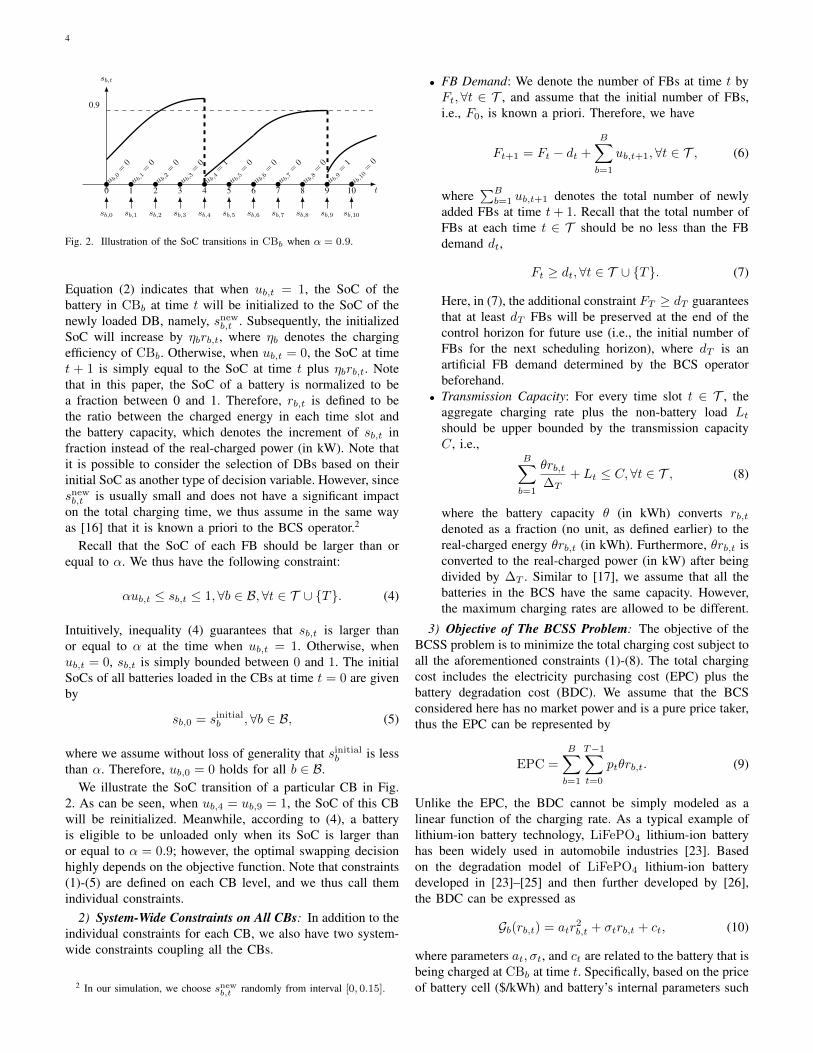
Fig. 2. Illustration of the SoC transitions in CBb when α = 0.9.

Equation (2) indicates that when ub,t = 1, the SoC of thebattery in CBb at time t will be initialized to the SoC of thenewly loaded DB, namely, snew

b,t . Subsequently, the initializedSoC will increase by ηbrb,t, where ηb denotes the chargingefficiency of CBb. Otherwise, when ub,t = 0, the SoC at timet + 1 is simply equal to the SoC at time t plus ηbrb,t. Notethat in this paper, the SoC of a battery is normalized to bea fraction between 0 and 1. Therefore, rb,t is defined to bethe ratio between the charged energy in each time slot andthe battery capacity, which denotes the increment of sb,t infraction instead of the real-charged power (in kW). Note thatit is possible to consider the selection of DBs based on theirinitial SoC as another type of decision variable. However, sincesnewb,t is usually small and does not have a significant impact

on the total charging time, we thus assume in the same wayas [16] that it is known a priori to the BCS operator.2

Recall that the SoC of each FB should be larger than orequal to α. We thus have the following constraint:

αub,t ≤ sb,t ≤ 1,∀b ∈ B,∀t ∈ T ∪ {T}. (4)

Intuitively, inequality (4) guarantees that sb,t is larger thanor equal to α at the time when ub,t = 1. Otherwise, whenub,t = 0, sb,t is simply bounded between 0 and 1. The initialSoCs of all batteries loaded in the CBs at time t = 0 are givenby

sb,0 = sinitialb ,∀b ∈ B, (5)

where we assume without loss of generality that sinitialb is less

than α. Therefore, ub,0 = 0 holds for all b ∈ B.We illustrate the SoC transition of a particular CB in Fig.

2. As can be seen, when ub,4 = ub,9 = 1, the SoC of this CBwill be reinitialized. Meanwhile, according to (4), a batteryis eligible to be unloaded only when its SoC is larger thanor equal to α = 0.9; however, the optimal swapping decisionhighly depends on the objective function. Note that constraints(1)-(5) are defined on each CB level, and we thus call themindividual constraints.

2) System-Wide Constraints on All CBs: In addition to theindividual constraints for each CB, we also have two system-wide constraints coupling all the CBs.

2 In our simulation, we choose snewb,t randomly from interval [0, 0.15].

• FB Demand: We denote the number of FBs at time t byFt,∀t ∈ T , and assume that the initial number of FBs,i.e., F0, is known a priori. Therefore, we have

Ft+1 = Ft − dt +

B∑

b=1

ub,t+1,∀t ∈ T , (6)

where∑Bb=1 ub,t+1 denotes the total number of newly

added FBs at time t+ 1. Recall that the total number ofFBs at each time t ∈ T should be no less than the FBdemand dt,

Ft ≥ dt,∀t ∈ T ∪ {T}. (7)

Here, in (7), the additional constraint FT ≥ dT guaranteesthat at least dT FBs will be preserved at the end of thecontrol horizon for future use (i.e., the initial number ofFBs for the next scheduling horizon), where dT is anartificial FB demand determined by the BCS operatorbeforehand.

• Transmission Capacity: For every time slot t ∈ T , theaggregate charging rate plus the non-battery load Ltshould be upper bounded by the transmission capacityC, i.e.,

B∑

b=1

θrb,t∆T

+ Lt ≤ C,∀t ∈ T , (8)

where the battery capacity θ (in kWh) converts rb,tdenoted as a fraction (no unit, as defined earlier) to thereal-charged energy θrb,t (in kWh). Furthermore, θrb,t isconverted to the real-charged power (in kW) after beingdivided by ∆T . Similar to [17], we assume that all thebatteries in the BCS have the same capacity. However,the maximum charging rates are allowed to be different.

3) Objective of The BCSS Problem: The objective of theBCSS problem is to minimize the total charging cost subject toall the aforementioned constraints (1)-(8). The total chargingcost includes the electricity purchasing cost (EPC) plus thebattery degradation cost (BDC). We assume that the BCSconsidered here has no market power and is a pure price taker,thus the EPC can be represented by

EPC =

B∑

b=1

T−1∑

t=0

ptθrb,t. (9)

Unlike the EPC, the BDC cannot be simply modeled as alinear function of the charging rate. As a typical example oflithium-ion battery technology, LiFePO4 lithium-ion batteryhas been widely used in automobile industries [23]. Basedon the degradation model of LiFePO4 lithium-ion batterydeveloped in [23]–[25] and then further developed by [26],the BDC can be expressed as

Gb(rb,t) = atr2b,t + σtrb,t + ct, (10)

where parameters at, σt, and ct are related to the battery that isbeing charged at CBb at time t. Specifically, based on the priceof battery cell ($/kWh) and battery’s internal parameters such

5

as voltage, current, and SoC, all of these three parameters canbe determined3. Therefore, the total BDC can be calculated as

BDC =

B∑

b=1

T−1∑

t=0

Gb(rb,t) (11)

Therefore, based on the EPC model and the BDC model, theBCSS problem can be formally formulated as the followingoptimization problem:

(BCSS)

{min EPC + BDC

s.t. (1)− (8),(12)

variables: {rb,t}∀b∈B,∀t∈T , {ub,t}∀b∈B,∀t∈T \{0}∪{T}.A quick observation for Problem (12) is that all constraints

are linear except (2), which consists of multiplication betweencontinuous and binary decision variables. Moreover, from(4) we can see that ub,t = 1 is feasible if and only ifα ≤ sb,t ≤ 1. Meanwhile, the SoC transition in (2) showsthat sb,t depends on rb,t′ with t′ ≤ t. Therefore, all therb,t′ with t′ ≤ t are strongly coupled with ub,t. The mixed-integer nature, the nonlinearity of the SoC transition, and thestrong coupling effect between the binary and the continuousdecision variables make Problem (12) difficult to solve. Thefollowing two sections aim to present a computationally-tractable algorithm to solve Problem (12). Before leaving thissection, the following two remarks provide some justificationabout the generality and feasibility issue of the BCSS problem.

Remark 1 (Generality of the BCSS Problem). Note that theBCSS problem is a mixed-integer nonlinear program (MINLP).In particular, when we adopt the quadratic BDC model (11)for typical LiFePO4 lithium-ion batteries, the BCSS problembecomes a mixed-integer quadratic program (MIQP). Consid-ering the wide application of LiFePO4 in EVs, we focus on thequadratic BDC model (11) in this paper and aim to solve theMIQP problem (12) hereinafter. However, it is worth pointingout that our BCSS problem can be any general MIP when othernonlinear/linear battery degradation models are introduced orother application scenarios are considered4. Meanwhile, ourproposed algorithm in the following sections is independentof the quadratic BDC model, as long as the objective functionof the MINLP problem is convex.

Remark 2 (Feasibility of the BCSS Problem). It is possiblethat the proposed BCSS problem is infeasible if the FB demandis very high. However, we consider that this is a planningproblem that should ensure the BCSS problem is feasiblebefore our proposed scheduling problem. For example, theBCS operator has to make a feasible commitment with BSSssuch that the total FB demand is within the capability of theBCS, or the BCS operator has to prepare enough FBs suchthat a given FB demand can be satisfied. Since the planningof a proper BCS is not the focus of this paper, we assumethat the BCSS problem is already feasible and focus on thescheduling aspect by proposing an efficient algorithm.

3The detailed expressions for ab,t, σb,t, and cb,t are referred to [26].4For instance, in addition to the cost minimization model proposed in

Problem (12), the BCS operator can also control the aggregate charging rateof the BCS to provide grid services such as peak-shaving and/or frequencyregulation service, etc.

III. AN EXACT ALGORITHM BASED ONGENERALIZED BENDERS DECOMPOSITION

In this section, we first show how to transform Problem (12)into a standard MIQP problem. We then propose to solve theMIQP problem with the GBD approach.

A. Standard MIQP Representation

We first represent the nonlinear constraint (2) as equivalentlinear constraints. Similar to [27] , for any b ∈ B and t ∈T ∪{T}, we define yb,t = sb,t(1−ub,t) as an auxiliary variableand rewrite (2) as

sb,t+1 = yb,t + ηbrb,t + snewb,t ub,t, t ∈ T . (13)

To preserve the equivalence between (13) and (2), the auxiliaryvariable yb,0 should be equal to sb,0 since ub,0 = 0 holds forall b ∈ B. Meanwhile, for all t ∈ T \{0} ∪ {T}, yb,t mustsatisfy the following linear inequalities :

yb,t ≤ yb,t−1 + ηbrb,t−1 + snewb,t−1ub,t−1, (14a)

yb,t ≥ yb,t−1 + ηbrb,t−1 + snewb,t−1ub,t−1 − ub,t, (14b)

yb,t ≤ 1− ub,t, (14c)yb,t ≥ 0. (14d)

The equivalence between (13)-(14d) and (2) can be checkedas follows: If ub,t = 0, constraints (14a) and (14b) guaranteethat yb,t = yb,t−1 + ηbrb,t−1 + snew

b,t−1ub,t−1 = sb,t = sb,t(1−ub,t), and in this case, constraints (14c) and (14d) are inactive.Otherwise, if ub,t = 1, constraints (14c) and (14d) guaranteethat yb,t = 0 = sb,t(1− ub,t), and similarly, constraints (14a)and (14b) are inactive. Therefore, constraints (13)-(14d) areindeed equivalent to (2). By utilizing this equivalence, wesubstitute (13) into constraint (4) and get the following twolinear inequality constraints for all t ∈ T \{0} ∪ {T}:

yb,t−1 + ηbrb,t−1 + snewb,t−1ub,t−1 ≤ 1, (15a)

yb,t−1 + ηbrb,t−1 + snewb,t−1ub,t−1 ≥ αub,t. (15b)

After the above transformation, (2) and (4) can be equiva-lently represented by (14a)-(15b). For compactness, we de-fine the following vectors to represent the decision vari-ables: rᵀb =

(rb,0, · · · , rb,T−1

),yᵀb =

(yb,1, · · · , yb,T

), and

uᵀb = (ub,1, · · · , ub,T ),∀b ∈ B. Thus, the above five linear

constraints (14a)-(14c), (15a), and (15b) can be combined intoone linear constraint as follows:

Abrb + Dbyb + Ebub ≤ fb,∀b ∈ B, (16)

where matrices {Ab}∀b∈B, {Db}∀b∈B, and {Eb}∀b∈B, andvector {fb}∀b∈B can be readily obtained by the correspondingcoefficients in (14a)-(14c), (15a), and (15b). Similarly, we canrepresent constraints (6), (7), and (8) as

B∑

b=1

Gbub ≥ d,

B∑

b=1

rb ≤ g, (17)

where matrix Gb consists of only 0 and 1, d = (dt)∀t, and g =( (C−Lt)∆T

θ

)∀t. Note that the first inequality constraint in (17)

corresponds to (6) and (7), and the second one corresponds to(8). Therefore, Problem (12) can be finally represented as a

6

standard MIQP problem with all linear constraints as follows:

min

B∑

b=1

[1

2rᵀbQbrb + pᵀrb

](18a)

s.t. (16) and (17), (18b)

0 ≤ rb ≤ rmaxb ,yb ≥ 0,ub ∈ {0, 1}T×1,∀b ∈ B, (18c)

variables: rb,yb,ub,∀b ∈ B, (18d)

where Qb is a diagonal matrix, p is the vector compoundedby θpt∆T and the linear term in Gb(rb,t), and rmax

b is a T ×1vector with all entries equal to rmax

b .After the above representation, Problem (18) can be directly

solved by commercial solvers such as Gurobi [34]. However,according to our numerical experiment, the computationaltime for directly solving Problem (18) with Gurobi 6.5.0[34] increases significantly even when B is larger than 50(details will be discussed in Section V). Therefore, instead ofdirectly solving Problem (18) with Gurobi, we will proposea more efficient algorithm by further exploiting the specialstructure of Problem (18). In particular, similar to [28], theGBD algorithm will be applied here and its details will bepresented in the following subsection. Note that in this paperwe focus on obtaining the exact solution of Problem (12).Those who are interested in obtaining an approximate solutionwith commercial solvers are referred to Appendix A.

B. The GBD Algorithm

In GBD, Problem (18) is partitioned into a master problemand a sub-problem. The resulting master problem is solved bya cutting plane algorithm in which, at each iteration, the binaryvariable of the master problem is first determined and the sub-problem is solved by fixing the binary variable. If the sub-problem is feasible and bounded, an optimality cut is addedto the master problem; otherwise a feasibility cut is added. Anupper bound can be computed from the feasible sub-problemand a lower bound can be obtained from the master problem.The process continues until an optimal solution is found or theoptimality gap is smaller than a given threshold. The wholeframework is presented in the following five steps:Step-1 (Initialization): Select a convergence

tolerance parameter ε ≥ 0. Set UB =∞ and LB = −∞. Setthe initial cut coefficients Φ1

b = Φ1b = 0, and Ψ1

b = Ψ1b = 0,

∀b ∈ B. Initialize K = 1 and L = 1 to count the numbers ofoptimality constraints and feasibility constraints, respectively.Step-2 (Master Problem): Solve the following

master problem:

minu,z

z

s.t.[Φk

1 , · · · ,ΦkB

]u +

B∑

b=1

Ψkb ≤ z,∀k = 1, · · · ,K, (19)

[Φ`

1, · · · , Φ`B

]u +

B∑

b=1

Ψ`b ≤ 0,∀` = 1, · · · , L, (20)

[G1, · · · ,GB

]u ≥ d,u ∈ {0, 1}T×B , (21)

where uᵀ = (uᵀ1 , · · · ,uᵀ

B). Let (uK , zK) be the optimalsolution, and set LB = zK . Terminate if UB ≤ LB + ε.

As will become clear later on, constraint (19) denotes the setof optimality cuts, which will push the lower bound LB closerto the optimal objective value of Problem (18). Meanwhile,constraint (20) represents the set of feasibility cuts, whichwill make uK more feasible for the sub-problem defined inProblem (22). In each iteration, the master problem will havea solution that is greater than or equal to the solution of theprevious iteration (i.e., the sequence of LB is non-decreasing).This is because constraints (19) and (20) will keep shrinkingthe space for searching u with the increase of K and L.Step-3 (Sub-problem): Given uK from Step-2,

Problem (18) reduces to a continuous optimization problemdefined on rb and yb,∀b ∈ B as follows:

Fsub(uK) = minrb,yb

B∑

b=1

[1

2rᵀbQbrb + pᵀrb

](22a)

s.t. Abrb + Dbyb ≤ fb −EbuKb ,∀b ∈ B, (22b)

B∑

b=1

rb ≤ g, (22c)

0 ≤ rb ≤ rmaxb ,yb ≥ 0,∀b ∈ B. (22d)

Problem (22) is often referred to as the Bender’s sub-problem, or sub-problem for short [29], [30]. Determinationof whether Problem (22) is feasible or not for a given uK canbe done by any Phase I algorithm. In particular, Floudas et al.in [30] proposed to solve the following linear programmingproblem:

Ffc(uK) = minrb,yb,δb

B∑

b=1

eᵀδb (23a)

s.t. Abrb + Dbyb ≤ fb −EbuKb + δb,∀b ∈ B, (23b)

B∑

b=1

rb ≤ g, (23c)

0 ≤ rb ≤ rmaxb ,yb ≥ 0, δb ≥ 0,∀b ∈ B, (23d)

where e = (1, 1, · · · , 1)ᵀ. Specifically, the feasibility of thesub-problem can be checked as follows: If Ffc(uK) = 0, uK

is feasible for the sub-problem. Otherwise, if Ffc(uK) > 0,the sub-problem is infeasible. Depending on the feasibility ofthe sub-problem, we have the following two steps.Step-4 (Optimality Cuts): If the sub-problem

(22) is feasible, let {rKb }∀b be its optimal primal solution andlet Fsub(uK) be the optimal objective value. Furthermore, wedualize constraint (22b) with Lagrange multiplier {λb}∀b andlet {λKb }∀b be the optimal dual solution. Note that the sub-problem is a convex optimization problem and constraint (22b)is separable in rb and uKb . Therefore, based on the standardconvex optimization theory, Fsub(uK) can be given as

Fsub(uK) =[ΦK+1

1 , · · · ,ΦK+1B

]uK +

B∑

b=1

ΨK+1b , (24)

7

where the two coefficients ΦK+1b and ΨK+1

b are computedbased on the optimal primal and dual variables as

ΦK+1b =

⟨λKb ,Eb

⟩,∀b ∈ B, (25)

ΨK+1b =

1

2

(rKb

)ᵀQbr

Kb + pᵀrKb +

⟨λKb ,Abr

Kb + Dby

Kb − fb

⟩,∀b ∈ B, (26)

We store (uK , (rKb )∀b) as the incumbent if Fsub(uK) isless than UB, and update the upper bound UB = Fsub(uK).If UB ≤ LB + ε, then we can claim that (uK , (rKb )∀b) is theoptimal solution for Problem (18) and terminate. Otherwise,increase K by 1 and go to Step-2.Step-5 (Feasibility Cuts): If the sub-problem

(22) is infeasible, then the feasibility cuts must be addedto the master problem. In particular, let {rLb }∀b, {yLb }∀b,and {δLb }∀b be the optimal primal solution for Problem (23),and let {λLb }∀b be the optimal dual solution associated withconstraint (23b). Since Problem (23) is a linear program, itsoptimal objective value Ffc(uK) is equivalent to the optimalobjective value of its dual problem written as follows:

Ffc(uK) =[ΦL+1

1 , · · · , ΦL+1B

]uK +

B∑

b=1

ΨL+1b , (27)

where the coefficients can be computed as

ΦL+1b =

⟨λLb ,Eb

⟩,∀b ∈ B, (28)

ΨL+1b =

⟨λLb ,Abr

Lb + Dby

Lb − fb

⟩,∀b ∈ B. (29)

After calculating the above two coefficients, increase L by 1and go to Step-2.

According to [29], the upper bound UB and the lowerbound LB will eventually converge to the same point if theoptimal solution is found, or become extremely close to eachother if the ε-optimal solution is located.5 It is worth pointingout that after performing the linearization in Section III-A,constraint (22b) is separable between uKb and rb, and linearin uKb . As a result, both the optimality cuts (19) and thefeasibility cuts (20) can be expressed as linear functions ofuKb . Therefore, the master problem remains as a mixed-integerlinear programming (MILP) problem (with only one contin-uous decision variable z). Transforming the original MIQPproblem into a series of MILP problems can significantly savethe computational time, as demonstrated by our simulationresults in Section V.

Note that in Step-4, we need to solve sub-problem (22)to obtain the optimal primal variable (rKb )∀b as well assolve its dual problem to obtain the optimal dual variable(λKb )∀b. Solving both the primal and dual of the sub-problemwith generic convex optimization solvers is definitely feasible.However, since we need to iteratively solve the sub-problem,solving this problem in an accurate and efficient way is criticalto the overall performance of the GBD method. Therefore, inthe next section, we will propose an efficient parallel algorithmfor solving the sub-problem.

5Note that as we mentioned in Step-2, the sequence of LB is non-decreasing. However, the sequence of the upper bound UB is not necessarilyto be non-increasing. More detailed explanation is referred to in [29].

IV. SOLVING SUB-PROBLEM (22) IN PARALLEL

In this section, we leverage the special decomposable struc-ture of the BCSS problem and propose an efficient parallelalgorithm for solving sub-problem (22). Our parallel algorithmconsists of two key procedures: i) the sub-problem is firstdecomposed into multiple individual sub-problems at each CBlevel based on dual decomposition (Subsection IV-A), and ii)each individual sub-problem is further partitioned into mul-tiple independent simple optimization problems (SubsectionIV-B). However, as some of the constraints are eliminatedduring the decomposition and partition processes, and thuswe further need to synthesize all the required dual variablesassociated with these constraints for calculating the optimalitycuts (Subsection IV-C). Lastly, we will discuss the parallelimplementation of our algorithm in Subsection IV-D.

A. Dual Decomposition of the Sub-Problem

Note that if we relax constraint (22c) with Lagrangemultiplier π, then all the CBs are decoupled. Specifi-cally, we have the Lagrange function L(r,y,uK ,π) =∑Bb=1

∑T−1t=0

[Gb(rb,t) + ptθrb,t∆T + πtrb,t

]− ∑T−1

t=0 πtgt,and thus the dual function can be written as G(π) =minr,y

L(r,y,uK ,π) =∑Bb=1 Sb(π)− 〈π,g〉, where Sb(π) is

the optimal objective value for the following individual sub-problem (I-Sub)6

(I-Sub) : minrb,yb

T−1∑

t=0

[Gb(rb,t) + (ptθ∆T + πt)rb,t

]

s.t. yb,t+1 ≤ yb,t + ηbrb,t + snewb,t u

Kb,t,∀t ∈ T , (λ1,b,t)

yb,t+1 ≥ yb,t + ηbrb,t + snewb,t u

Kb,t − uKb,t+1,∀t ∈ T , (λ2,b,t)

yb,t ≤ 1− uKb,t,∀t ∈ T ∪ {T}, (λ3,b,t)

yb,t + ηbrb,t + snewb,t u

Kb,t ≤ 1,∀t ∈ T ∪ {T}, (λ4,b,t)

yb,t + ηbrb,t + snewb,t u

Kb,t ≥ αuKb,t+1,∀t ∈ T ∪ {T}, (λ5,b,t)

0 ≤ rb,t ≤ rmaxb , yb,t+1 ≥ 0,∀t ∈ T ,

where the first five constraints correspond to constraint (22b)or equivalently (14a)-(14c) and (15a)-(15b), and the lastone constraint corresponds to constraint (22d). Note thatλ1,b,t, · · · , λ5,b,t are the respective dual variables associatedwith each corresponding constraint. Meanwhile, these five dualvariables are the respective entries of λb defined in Step-4,i.e., λb = (λ1,b,t, · · · , λ5,b,t)∀t.

The dual problem of the I-Sub problem is

maxπ

G(π), s.t. π ≥ 0, (30)

and the update of π at iteration n can follow the projectedgradient method:

π(n+ 1) =

[π(n) + σ

(B∑

b=1

rb(n)− g

)]+

. (31)

Since the I-Sub problem is a convex optimization problem, theLagrange multiplier π is guaranteed to converge to the optimalsolution, as long as the step-size σ is sufficiently small.

6By individual, we mean this optimization problem is defined at eachindividual CB level.

8

t

sb,t

α

snewb,t1

t = t1 t = t2

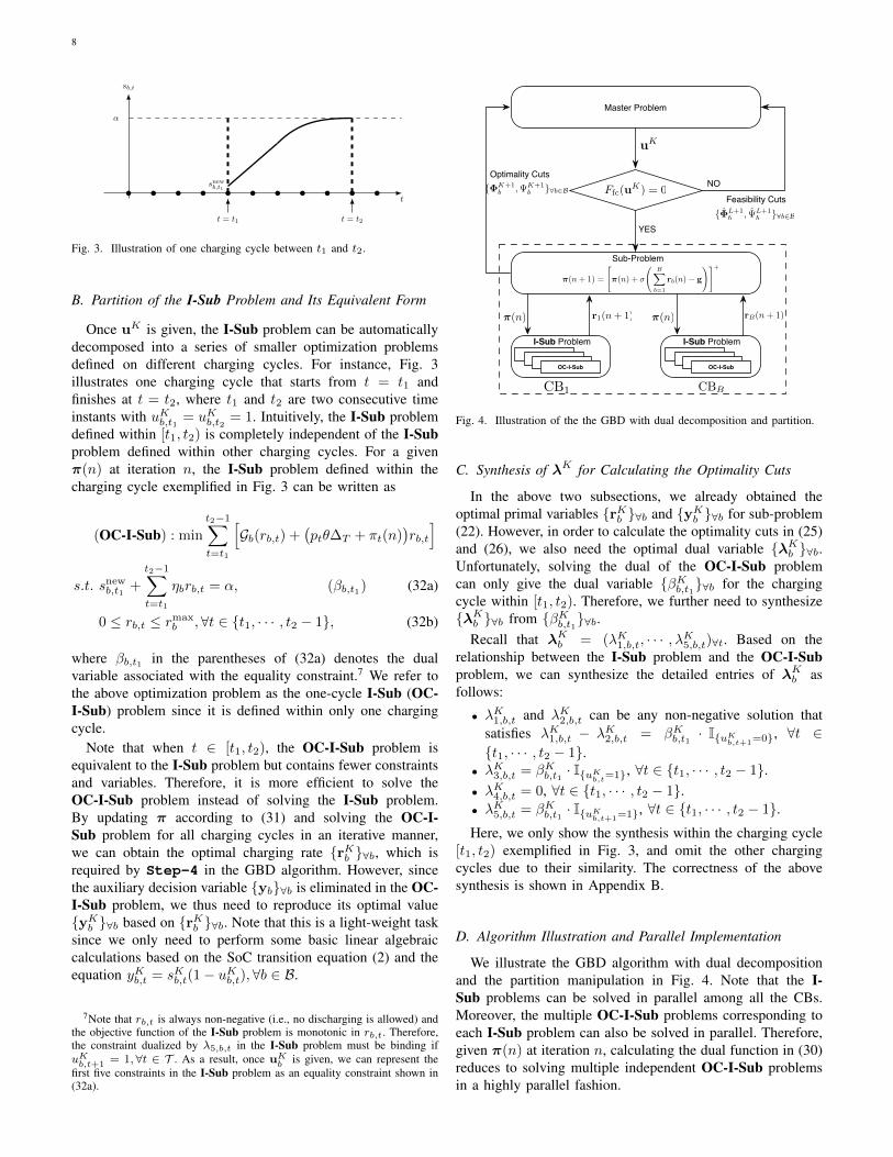
Fig. 3. Illustration of one charging cycle between t1 and t2.

B. Partition of the I-Sub Problem and Its Equivalent Form

Once uK is given, the I-Sub problem can be automaticallydecomposed into a series of smaller optimization problemsdefined on different charging cycles. For instance, Fig. 3illustrates one charging cycle that starts from t = t1 andfinishes at t = t2, where t1 and t2 are two consecutive timeinstants with uKb,t1 = uKb,t2 = 1. Intuitively, the I-Sub problemdefined within [t1, t2) is completely independent of the I-Subproblem defined within other charging cycles. For a givenπ(n) at iteration n, the I-Sub problem defined within thecharging cycle exemplified in Fig. 3 can be written as

(OC-I-Sub) : min

t2−1∑

t=t1

[Gb(rb,t) +

(ptθ∆T + πt(n)

)rb,t

]

s.t. snewb,t1 +

t2−1∑

t=t1

ηbrb,t = α, (βb,t1) (32a)

0 ≤ rb,t ≤ rmaxb ,∀t ∈ {t1, · · · , t2 − 1}, (32b)

where βb,t1 in the parentheses of (32a) denotes the dualvariable associated with the equality constraint.7 We refer tothe above optimization problem as the one-cycle I-Sub (OC-I-Sub) problem since it is defined within only one chargingcycle.

Note that when t ∈ [t1, t2), the OC-I-Sub problem isequivalent to the I-Sub problem but contains fewer constraintsand variables. Therefore, it is more efficient to solve theOC-I-Sub problem instead of solving the I-Sub problem.By updating π according to (31) and solving the OC-I-Sub problem for all charging cycles in an iterative manner,we can obtain the optimal charging rate {rKb }∀b, which isrequired by Step-4 in the GBD algorithm. However, sincethe auxiliary decision variable {yb}∀b is eliminated in the OC-I-Sub problem, we thus need to reproduce its optimal value{yKb }∀b based on {rKb }∀b. Note that this is a light-weight tasksince we only need to perform some basic linear algebraiccalculations based on the SoC transition equation (2) and theequation yKb,t = sKb,t(1− uKb,t),∀b ∈ B.

7Note that rb,t is always non-negative (i.e., no discharging is allowed) andthe objective function of the I-Sub problem is monotonic in rb,t. Therefore,the constraint dualized by λ5,b,t in the I-Sub problem must be binding ifuKb,t+1 = 1, ∀t ∈ T . As a result, once uK

b is given, we can represent thefirst five constraints in the I-Sub problem as an equality constraint shown in(32a).

Master Problem

Ffc(uK) = 0

I-Sub Problem I-Sub Problem

Optimality Cuts

Feasibility Cuts

⇡(n) ⇡(n) rB(n + 1)

⇡(n + 1) =

"⇡(n) + �

BX

b=1

rb(n) � g

!#+

Sub-Problem

uK

NO

YES

CB1 CBB

{�K+1b , K+1

b }8b2B

{�L+1b , L+1

b }8b2B

r1(n + 1)

Problem (28)Problem (28)Problem (28)OC-I-Sub

Problem (28)Problem (28)Problem (28)OC-I-Sub

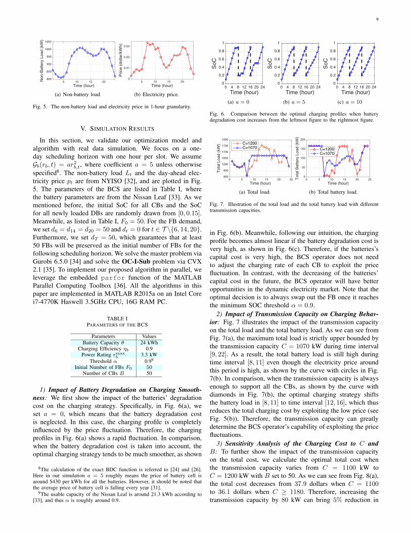
Fig. 4. Illustration of the the GBD with dual decomposition and partition.

C. Synthesis of λK for Calculating the Optimality Cuts

In the above two subsections, we already obtained theoptimal primal variables {rKb }∀b and {yKb }∀b for sub-problem(22). However, in order to calculate the optimality cuts in (25)and (26), we also need the optimal dual variable {λKb }∀b.Unfortunately, solving the dual of the OC-I-Sub problemcan only give the dual variable {βKb,t1}∀b for the chargingcycle within [t1, t2). Therefore, we further need to synthesize{λKb }∀b from {βKb,t1}∀b.

Recall that λKb = (λK1,b,t, · · · , λK5,b,t)∀t. Based on therelationship between the I-Sub problem and the OC-I-Subproblem, we can synthesize the detailed entries of λKb asfollows:

• λK1,b,t and λK2,b,t can be any non-negative solution thatsatisfies λK1,b,t − λK2,b,t = βKb,t1 · I{uK

b,t+1=0}, ∀t ∈{t1, · · · , t2 − 1}.

• λK3,b,t = βKb,t1 · I{uKb,t=1}, ∀t ∈ {t1, · · · , t2 − 1}.

• λK4,b,t = 0, ∀t ∈ {t1, · · · , t2 − 1}.• λK5,b,t = βKb,t1 · I{uK

b,t+1=1}, ∀t ∈ {t1, · · · , t2 − 1}.Here, we only show the synthesis within the charging cycle

[t1, t2) exemplified in Fig. 3, and omit the other chargingcycles due to their similarity. The correctness of the abovesynthesis is shown in Appendix B.

D. Algorithm Illustration and Parallel Implementation

We illustrate the GBD algorithm with dual decompositionand the partition manipulation in Fig. 4. Note that the I-Sub problems can be solved in parallel among all the CBs.Moreover, the multiple OC-I-Sub problems corresponding toeach I-Sub problem can also be solved in parallel. Therefore,given π(n) at iteration n, calculating the dual function in (30)reduces to solving multiple independent OC-I-Sub problemsin a highly parallel fashion.

9

5 10 15 20Time (hour)

800

850

900

950

1000

1050N

on-B

atte

ry L

oad

(kW

)

(a) Non-battery load.

5 10 15 20Time (hour)

0

0.01

0.02

0.03

Pric

e (d

olla

r/kW

h)

(b) Electricity price.

Fig. 5. The non-battery load and electricity price in 1-hour granularity.

V. SIMULATION RESULTS

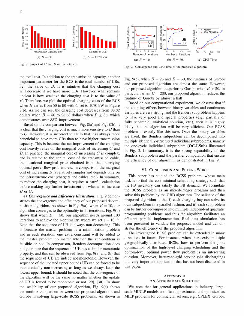
In this section, we validate our optimization model andalgorithm with real data simulation. We focus on a one-day scheduling horizon with one hour per slot. We assumeGb(rb, t) = ar2

b,t, where coefficient a = 5 unless otherwisespecified8. The non-battery load Lt and the day-ahead elec-tricity price pt are from NYISO [32], and are plotted in Fig.5. The parameters of the BCS are listed in Table I, wherethe battery parameters are from the Nissan Leaf [33]. As wementioned before, the initial SoC for all CBs and the SoCfor all newly loaded DBs are randomly drawn from [0, 0.15].Meanwhile, as listed in Table I, F0 = 50. For the FB demand,we set d6 = d14 = d20 = 50 and dt = 0 for t ∈ T \{6, 14, 20}.Furthermore, we set dT = 50, which guarantees that at least50 FBs will be preserved as the initial number of FBs for thefollowing scheduling horizon. We solve the master problem viaGurobi 6.5.0 [34] and solve the OC-I-Sub problem via CVX2.1 [35]. To implement our proposed algorithm in parallel, weleverage the embedded parfor function of the MATLABParallel Computing Toolbox [36]. All the algorithms in thispaper are implemented in MATLAB R2015a on an Intel Corei7-4770K Haswell 3.5GHz CPU, 16G RAM PC.

TABLE IPARAMETERS OF THE BCS

Parameters ValuesBattery Capacity θ 24 kWh

Charging Efficiency ηb 0.9Power Rating rmax

b 3.3 kWThreshold α 0.99

Initial Number of FBs F0 50Number of CBs B 50

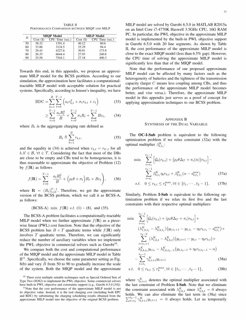
1) Impact of Battery Degradation on Charging Smooth-ness: We first show the impact of the batteries’ degradationcost on the charging strategy. Specifically, in Fig. 6(a), weset a = 0, which means that the battery degradation costis neglected. In this case, the charging profile is completelyinfluenced by the price fluctuation. Therefore, the chargingprofiles in Fig. 6(a) shows a rapid fluctuation. In comparison,when the battery degradation cost is taken into account, theoptimal charging strategy tends to be much smoother, as shown

8The calculation of the exact BDC function is referred to [24] and [26].Here in our simulation a = 5 roughly means the price of battery cell isaround $430 per kWh for all the batteries. However, it should be noted thatthe average price of battery cell is falling every year [31].

9The usable capacity of the Nissan Leaf is around 21.3 kWh according to[33], and thus α is roughly around 0.9.

0 4 8 12 16 20 24Time (hour)

0

0.2

0.4

0.6

0.8

1

SoC

(a) a = 0

0 4 8 12 16 20 24Time (hour)

0

0.2

0.4

0.6

0.8

1

SoC

(b) a = 5

0 4 8 12 16 20 24Time (hour)

0

0.2

0.4

0.6

0.8

1

SoC

(c) a = 10

Fig. 6. Comparison between the optimal charging profiles when batterydegradation cost increases from the leftmost figure to the rightmost figure.

0 5 10 15 20 25Time (hour)

900

950

1000

1050

1100

1150

1200

Tota

l Loa

d (k

W) C=1200

C=1070

(a) Total load.

0 5 10 15 20 25Time (hour)

0

50

100

150

200

Tota

l Bat

tery

Loa

d (k

W)

C=1200C=1070

(b) Total battery load.

Fig. 7. Illustration of the total load and the total battery load with differenttransmission capacities.

in Fig. 6(b). Meanwhile, following our intuition, the chargingprofile becomes almost linear if the battery degradation cost isvery high, as shown in Fig. 6(c). Therefore, if the batteries’scapital cost is very high, the BCS operator does not needto adjust the charging rate of each CB to exploit the pricefluctuation. In contrast, with the decreasing of the batteries’capital cost in the future, the BCS operator will have betteropportunities in the dynamic electricity market. Note that theoptimal decision is to always swap out the FB once it reachesthe minimum SOC threshold α = 0.9.

2) Impact of Transmission Capacity on Charging Behav-ior: Fig. 7 illustrates the impact of the transmission capacityon the total load and the total battery load. As we can see fromFig. 7(a), the maximum total load is strictly upper bounded bythe transmission capacity C = 1070 kW during time interval[9, 22]. As a result, the total battery load is still high duringtime interval [8, 11] even though the electricity price aroundthis period is high, as shown by the curve with circles in Fig.7(b). In comparison, when the transmission capacity is alwaysenough to support all the CBs, as shown by the curve withdiamonds in Fig. 7(b), the optimal charging strategy shiftsthe battery load in [8, 11] to time interval [12, 16], which thusreduces the total charging cost by exploiting the low price (seeFig. 5(b)). Therefore, the transmission capacity can greatlydetermine the BCS operator’s capability of exploiting the pricefluctuations.

3) Sensitivity Analysis of the Charging Cost to C andB: To further show the impact of the transmission capacityon the total cost, we calculate the optimal total cost whenthe transmission capacity varies from C = 1100 kW toC = 1200 kW with B set to 50. As we can see from Fig. 8(a),the total cost decreases from 37.9 dollars when C = 1100to 36.1 dollars when C ≥ 1180. Therefore, increasing thetransmission capacity by 80 kW can bring 5% reduction in

10

1100 1120 1140 1160 1180 1200Transmission Capacity (kW)

35

35.5

36

36.5

37

37.5

38To

tal C

ost (

dolla

rs)

(a) B = 50

50 60 70 80 90Number of CBs

20

25

30

35

40

Tota

l Cos

t (do

llars

)

(b) C = 1070 kW

Fig. 8. Impact of C and B on the total cost.

the total cost. In addition to the transmission capacity, anotherimportant parameter for the BCS is the total number of CBs,i.e., the value of B. It is intuitive that the charging costwill decrease if we have more CBs. However, what remainsunclear is how sensitive the charging cost is to the value ofB. Therefore, we plot the optimal charging costs of the BCSwhen B varies from 50 to 90 with C set to 1070 kW in Figure8(b). As we can see, the charging cost decreases from 38.32dollars when B = 50 to 25.58 dollars when B ≥ 85, whichdemonstrates over 33% improvement.

Based on the comparison between Fig. 8(a) and Fig. 8(b), itis clear that the charging cost is much more sensitive to B thanto C. However, it is incorrect to claim that it is always morebeneficial to have more CBs than to have higher transmissioncapacity. This is because the net improvement of the chargingcost heavily relies on the marginal costs of increasing C andB. In practice, the marginal cost of increasing C is complex,and is related to the capital cost of the transmission cable,the locational marginal price obtained from the underlyingoptimal power flow problem, etc. In comparison, the marginalcost of increasing B is relatively simpler and depends only onthe infrastructure cost (chargers and cables, etc.). In summary,to reduce the charging cost, it requires a careful calculationbefore making any further investment on whether to increaseB or C.

4) Convergence and Efficiency Illustration: Fig. 9 demon-strates the convergence and efficiency of our proposed decom-position algorithm. As shown in Fig. 9(a), when B = 10, ouralgorithm converges to the optimality in 11 iterations. Fig. 9(b)shows that when B = 50, our algorithm needs around 100iterations to achieve the ε-optimality, where we set ε = 10−3.Note that the sequence of LB is always non-decreasing. Thisis because the master problem is a minimization problemand in each iteration, one extra constraint will be added tothe master problem no matter whether the sub-problem isfeasible or not. In comparison, Benders decomposition doesnot guarantee that the sequence of UB has a similar monotonicproperty, and this can be observed from Fig. 9(a) and (b) thatthe sequences of UB are indeed not monotonic. However, thesequence of the updated upper bounds UB can be forced to bemonotonically non-increasing as long as we always keep thelowest upper bound. It should be noted that the convergence ofthe algorithm will be the same no matter whether the updateof UB is forced to be monotonic or not [29], [30]. To showthe scalability of our proposed algorithm, Fig. 9(c) showsthe runtime comparison between our proposed algorithm andGurobi in solving large-scale BCSS problems. As shown in

2 4 6 8 10 12Number of Iterations

-10

-5

0

5

10

Tota

l Cos

t (do

llars

)

UBLB

(a) B = 10.

0 50 100 150Number of Iterations

16

21

26

31

36

41

Tota

l Cos

t (do

llars

)

UBLB

(b) B = 50.

25 75 125 175B

0

1

2

3

4

Run

time

(hou

r) GurobiOur Algorithm

(c) CPU Time.

Fig. 9. Convergence and CPU time of the proposed algorithm.

Fig. 9(c), when B = 25 and B = 50, the runtimes of Gurobiand our proposed algorithm are almost the same. However,our proposed algorithm outperforms Gurobi when B > 50. Inparticular, when B = 200, our proposed algorithm reduces theruntime of Gurobi by almost a half.

Based on our computational experiment, we observe that ifthe coupling effects between binary variables and continuousvariables are very strong, and the Benders subproblem happensto have very good and special properties (e.g., partially orfully separable, analytical solution, etc.), then it is highlylikely that the algorithm will be very efficient. Our BCSSproblem is exactly like this case. Once the binary variablesare fixed, the Benders subproblem can be decomposed intomultiple identically-structured individual subproblems, namelythe one-cycle individual subproblem (OC-I-Sub) illustratedin Fig. 3. In summary, it is the strong separability of theBenders subproblem and the parallel computation that ensurethe efficiency of our algorithm, as demonstrated in Fig. 9.

VI. CONCLUSION AND FUTURE WORK

This paper has studied the BCSS problem, whose maintask is to find the cost-minimal scheduling strategy such thatthe FB inventory can satisfy the FB demand. We formulatethe BCSS problem as an mixed-integer program and thensolve this problem by the GBD algorithm. The salience of theproposed algorithm is that i) each charging bay can solve itsown subproblem in a parallel fashion, and ii) each subproblemcan be further decomposed into multiple independent quadraticprogramming problems, and thus the algorithm facilitates anefficient parallel implementation. Real data simulation hasbeen presented to validate the proposed model and demon-strates the efficiency of the proposed algorithm.

The investigated BCSS problem can be extended in manydirections in future. For instance, when there exist multiplegeographically-distributed BCSs, how to perform the jointoptimization of the high-level charging scheduling and thebottom-level optimal power flow problem is an interestingquestion. Moreover, battery-to-grid service (via discharging)is a very important application that has not been discussed inthis paper.

APPENDIX AAN APPROXIMATE SOLUTION

We note that for general applications in industry, large-scale MINLP models are often approximated and optimized asMILP problems for commercial solvers, e.g., CPLEX, Gurobi.

11

TABLE IIPERFORMANCE COMPARISON BETWEEN MIQP AND MILP

BMIQP Model MILP Model

Cost ($) CPU Time (sec.) Cost ($) CPU Time (sec.)50 38.32 1391.4 40.12 60.660 33.86 3124.5 35.29 94.470 29.43 4227.6 30.91 173.980 26.35 6644.4 27.93 240.890 25.58 7544.1 27.18 400.3

Towards this end, in this appendix, we propose an approxi-mate MILP model for the BCSS problem. According to oursimulation, the approximation here facilitates a computational-tractable MILP model with acceptable solution for practicalsystems. Specifically, according to Jensen’s inequality, we have

BDC =

B∑

b=1

T−1∑

t=0

(atr

2b,t + σtrb,t + ct

)(33)

≥T−1∑

t=0

atR2t

B+

T−1∑

t=0

σtRt +

T−1∑

t=0

Bct, (34)

where Rt is the aggregate charging rate defined as

Rt ,B∑

b=1

rb,t, (35)

and the equality in (34) is achieved when rb,t = rb′,t for allb, b′ ∈ B, ∀t ∈ T . Considering the fact that most of the DBsare close to be empty and CBs tend to be homogeneous, it isthus reasonable to approximate the objective of Problem (12)by f(R) as follows

f(R) =

T−1∑

t=0

(atR

2t

B+(ptθ + σt

)Rt +Bct

), (36)

where R = (Rt)T−1t=0 . Therefore, we get the approximate

version of the BCSS problem, which we call it as BCSS-A,as follows:

(BCSS-A) min f(R) s.t. (1)− (8), and (35).

The BCSS-A problem facilitates a computationally-tractableMILP model when we further approximate f(R) as a piece-wise linear (PWL) cost function. Note that the objective of theBCSS problem has B × T quadratic terms while f(R) onlyinvolves T quadratic terms. Therefore, we can significantlyreduce the number of auxiliary variables when we implementthe PWL objective in commercial solvers such as Gurobi10.

We compare both the cost and computational performanceof the MIQP model and the approximate MILP model in TableII11. Specifically, we choose the same parameter setting as Fig.8(b) and vary B from 50 to 90 to gradually increase the scaleof the system. Both the MIQP model and the approximate

10 There exist multiple suitable techniques such as Special Ordered Sets ofType Two (SOS2) to implement the PWL objective. Some commercial solvershave built-in PWL objective and constraints support (e.g., Gurobi 6.5.0 [34]).

11Note that the cost performance of the approximate MILP model is notits objective value. Instead, it is the real charging cost (including both EPCand BDC) by substituting the charging scheduling results obtained from theapproximate MILP model into the objective of the original BCSS problem.

MILP model are solved by Gurobi 6.5.0 in MATLAB R2015aon an Intel Core i7-4770K Haswell 3.5GHz CPU, 16G RAMPC. In particular, the PWL objective in the approximate MILPmodel is implemented by the built-in PWL objective supportin Gurobi 6.5.0 with 20 line segments. As shown by TableII, the cost performance of the approximate MILP model isclose to the exact MIQP model (less than 6.5% gap). However,the CPU time of solving the approximate MILP model issignificantly less than that of the MIQP model.

Note that the performance of our proposed approximateMILP model can be affected by many factors such as theheterogeneity of batteries and the tightness of the transmissioncapacity (larger C means less coupling among CBs, and thusthe performance of the approximate MILP model becomesbetter, and vise versa.). Therefore, the approximate MILPmodel in this appendix just serves as a proof of concept forapplying approximation techniques to our BCSS problem.

APPENDIX BSYNTHESIS OF THE DUAL VARIABLE

The OC-I-Sub problem is equivalent to the followingoptimization problem if we relax constraint (32a) with theoptimal multiplier βKb,t1 :

min

t2−1∑

t=t1

[Gb(rb,t) +

(ptθ∆T + πt(n)

)rb,t

]−

t2−1∑

t=t1

βKb,t1ηbrb,t + βKb,t1(α− snewb,t1 ) (37a)

s.t. 0 ≤ rb,t ≤ rmaxb ,∀t ∈ {t1, · · · , t2 − 1}. (37b)

Similarly, Problem I-Sub is equivalent to the following op-timization problem if we relax its first five and the lastconstraints with their respective optimal multipliers:

min

t2−1∑

t=t1

[Gb(rb,t) + (ptθ∆T + πt)rb,t

]+

(λK1,b,t1 − λK2,b,t1)(yb,t1+1 − yb,t1 − ηbrb,t1 − snew

b,t1

)+

t2−2∑

t=t1+1

(λK1,b,t − λK2,b,t)(yb,t+1 − yb,t − ηbrb,t

)+

λK3,b,t1yb,t1 − λK5,b,t2−1

(yb,t2−1 + ηbrb,t2−1 − α

)

−t2−1∑

t=t1

γKb,t+1yb,t+1 (38a)

s.t. 0 ≤ rb,t ≤ rmaxb ,∀t ∈ {t1, · · · , t2 − 1}, (38b)

where γKb,t+1 denotes the optimal multiplier associated withthe last constraint of Problem I-Sub. Note that we eliminatethe constraint associated with λK4,b,t since λK4,b,t = 0 alwaysholds. We can also eliminate the last term in (38a) since∑t2−1t=t1

γKb,t+1yb,t+1 = 0 always holds. Let us temporarily

12

ignore the first term in (38a) and rearrange the order of theremaining terms as

λK3,b,t1yb,t1 + (λK1,b,t1 − λK2,b,t1)(yb,t1+1 − yb,t1

)+

t2−2∑

t=t1+1

(λK1,b,t − λK2,b,t)(yb,t+1 − yb,t

)− λK5,b,t2−1yb,t2−1

− (λK1,b,t1 − λK2,b,t1)ηbrb,t1 −t2−2∑

t=t1+1

(λK1,b,t − λK2,b,t)ηbrb,t−

λK5,b,t2−1ηbrb,t2−1 + λK5,b,t2−1α− (λK1,b,t1 − λK2,b,t1)snewb,t1 .

(39)

Note that if λK1,b,t − λK2,b,t = λK3,b,t1 = λK5,b,t2−1 = βKb,t1 ,∀t ∈ {t1, · · · , t2 − 2}, (39) can be equivalently simplified tothe following formula

−t2−1∑

t=t1

βKb,t1ηbrb,t + βKb,t1(α− snewb,t1 ), (40)

which is the same as the last two terms in the objectivefunction of Problem (37). Therefore, the optimal dual variableλKb can indeed be synthesized according to the followingmethod:• λK1,b,t and λK2,b,t can be any non-negative solution that

satisfies λK1,b,t − λK2,b,t = βKb,t1 · I{uKb,t+1=0}, ∀t ∈

{t1, · · · , t2 − 1}.• λK3,b,t = βKb,t1 · I{uK

b,t=1}, ∀t ∈ {t1, · · · , t2 − 1}.• λK4,b,t = 0, ∀t ∈ {t1, · · · , t2 − 1}.• λK5,b,t = βKb,t1 · I{uK

b,t+1=1}, ∀t ∈ {t1, · · · , t2 − 1}.For other charging cycles, e.g., a charging cycle that starts

from t = t′1 and ends at t = t′2, we will obtain another optimaldual variable βKb,t′1 , and the the same approach can be appliedto synthesize λKb within this charging cycle. After visiting allthe charging cycles, all the entries of λKb can be synthesized.

REFERENCES

[1] E. Ungar and K. Fell, “Plug in, turn on, and load up,” IEEE PowerEnergy Mag., vol. 8, no. 3, pp. 30-35, May.-Jun., 2010.

[2] M. Yilmaz and P.T. Krein, “Review of battery charger topologies,charging power levels, and infrastructure for plug-in electric and hybridvehicles,” IEEE Trans. Power Electron., vol.28, no. 5, pp. 2151-2169,2012.

[3] Battery Swapping Project for Electric Buses in Qingdao, China.[Online]. Available: http://www.electronicsnews.com.au/features/battery-swapping-becoming-common-practice-for-comm.

[4] J. Kim, I. Song, and W. Choi, “An electric bus with a battery exchangesystem,” Energies, vol 8, no. 7, pp. 6806-6819, July 2015.

[5] A. Kuperman, U. Levy, J. Goren, A. Zafransky, and A. Savernin,“Battery charger for electric vehicle traction battery switch station, IEEETrans. Ind. Electron., vol. 60, no. 12, pp. 5391-5399, Dec. 2013.

[6] [Online]. Available: http://www.technologyreview.com/news/516276/why-tesla-thinks-it-can-make-battery-swapping-work/

[7] H. Mak, Y. Rong, and Z.M. Shen, “Infrastructure planning for electricvehicles with battery swapping,” Management Science, vol. 59, no. 7,pp. 1557-1575, July 2013.

[8] Y. Miao, Q. Jiang, and Y. Cao, “Battery switch station modeling and itseconomic evaluation in microgrid,” IEEE PES General Meeting, 2012.

[9] M. Takagi, Y. Iwafune, H. Yamamoto, K. Yamaji, K. Okano, R. Hiwatari,and T. Ikeya, “Economic value of PV energy storage using batteries ofbattery switch stations, IEEE Trans. Sust. Energy, vol. 4, no. 1, pp.164-173, Jan. 2013.

[10] P. Lombardi, M. Heuer, Z. Styczynski. “Battery switch station as storagesystem in an autonomous power system: Optimization issue,” IEEE PESGeneral Meeting, 2010.

[11] B. Avci, K. Girotra, and S. Netessine, “Electric vehicles with a batteryswitching station: adoption and environmental impact,” ManagementScience, vol. 61, no. 4, pp. 772-794, April 2015.

[12] L. Cheng, Y. Chang, J. Lin and C. Singh, “Power system reliabilityassessment with electric vehicle integration using battery exchangemode,” IEEE Trans. Sustainable Energy, vol. 4, No. 4, Oct. 2013.

[13] Y. Zheng, Z. Dong, Y. Xu, K. Meng, J. Zhao and J. Qiu, “Electric vehiclebattery charging/swap stations in distribution systems: Comparison studyand optimal planning,” IEEE Trans. Power System, vol. 29, no. 1, 2014.

[14] B. Sun, X. Tan and D.H.K Tsang, “Optimal operation of BSSs withQoS guarantee,” IEEE SmartGridComm 2014, Venice, Italy, Nov. 2014.

[15] S. Nurre, R. Bent, F. Pan, T. Sharkey, “Managing operations of plug-inhybrid electric vehicle (PHEV) exchange stations for use with a smartgrid”. Energy Policy, vol. 67, pp. 364-377, April 2014.

[16] M. Sarker, H. Pandzic, M. Ortega-Vazquez, “Optimal operation andservices scheduling for an electric vehicle battery swapping station,”IEEE Trans. Power Syst., vol. 30, no. 2, pp. 901-910, July 2015.

[17] P. You, Z. Yang, Y. Zhang, S. Low, Y. Sun, “Optimal charging schedulefor a battery switching station serving electric buses,” IEEE Trans. PowerSystems, vol. 31, no. 5, pp. 3473-3483, Sept. 2016.

[18] R. Widrick, S. Nurre, and M. Robbins, “Optimal policies for themanagement of an electric vehicle battery swap station,” to appear inTransp. Sci., 2016.

[19] O. Worley and D. Klabjan, “Optimization of battery charging anpurchasing at electric vehicle battery swap stations,” in Proc. 2011 IEEEVehicle Power and Propulsion Conf., pp. 1-4, 2011.

[20] T. Raviv, “The battery switching station scheduling problem,” Opera-tions Research Letters, vol. 40, no. 6, pp. 546-550, June 2012.

[21] B. Sun, Zhe Huang, X. Tan, and D.H.K. Tsang, “Optimal schedulingfor electric vehicle charging with discrete charging levels in distributiongrid,” accepted by IEEE Transactions on Smart Grid, 2016.

[22] I. Dincer, H.S. Hamut, N. Javani, “Thermal Management of ElectricVehicle Battery Systems,” Automotive Series, Wiley, 2017.

[23] J. Forman, J. Stein, H. Fathy, “Optimization of dynamic batteryparameter characterization experiments via differential evolution,” inproceedings of American Control Conference, pp. 867-874, Washington,DC, USA, 2013.

[24] J. Forman, S. Moura, J. Stein, H. Fathy, “Optimal experimental designfor modeling battery degradation,” in Proceedings of Dynamic Systemsand Control Conference, pp. 309318, 2012.

[25] S. Moura, J. Forman, S. Bashash, J. Stein, H. Fathy, “Optimal controlof film growth in lithium-ion battery packs via relay switches,” IEEETrans. Industrial Electronics, vol. 58, no. 8, pp. 3555-3566, 2011.

[26] Z. Ma, S. Zou, L. Ran, X. Shi and I.A. Hiskens, “Efficient decentralizedcoordination of large-scale plug-in electric vehicle charging,” Automat-ica, vol. 69, pp. 35-47, 2016.

[27] C. P. Christelle and M. Sevaux, Applications of optimization withXpressMP, 2002.

[28] Z. Yang, K. Long, P. You, and M.Y. Chow, “Joint Scheduling of Large-Scale Appliances and Batteries via Distributed Mixed Optimization,”IEEE Trans. Power Systems, vol. 30, no. 4, pp. 2031-2040, Jul. 2015.

[29] A. Geoffrion, “Generalized benders decomposition,” Journal of Opti-mization Theory and Applications, vol. 10, no. 4, pp. 237-260, 1972.

[30] C. Floudas, A. Aggarwal, and A. Ciric, “Global optimum search fornonconvex NLP and MINLP problems,” Computers and ChemicalEngineering, no. 10, pp. 1117-1132, 1989.

[31] [Online]. Available: https://electrek.co/2017/01/30/electric-vehicle-battery-cost-dropped-80-6-years-227kwh-tesla-190kwh/.

[32] [Online]. Available: http://www.nyiso.com/public/markets operations/market data/pricing data/index.jsp.

[33] [Online]. Available: https://en.wikipedia.org/wiki/Nissan Leaf.[34] Gurobi Optimization. [Online]. Available: http://www.gurobi.com/[35] CVX Research Inc. [Online]. Available: http://cvxr.com/cvx/[36] G. Sharma and J. Martin, “MATLABr: A language for parallel com-

puting,” Int. J. Parallel Program., vol.37, no. 1, pp. 336, 2009.