Economic Modelling 41 (2014) 319–328

Contents lists available at ScienceDirect

Economic Modelling

j ourna l homepage: www.e lsev ie r .com/ locate /ecmod

Optimal stopping time with stochastic volatility

Ran Zhang a,⁎, Shuang Xu b

a Department of Finance, Dongling School of Economics and Management, University of Science and Technology Beijing, PR Chinab Yibin City Commercial Bank of Sichuan Province, PR China

⁎ Corresponding author at: Office 1210, Guanli BuildingDistrict, Beijing 100083, PR China. Tel.: +86 1510106926

E-mail address: rzhang@ustb.edu.cn (R. Zhang).

http://dx.doi.org/10.1016/j.econmod.2014.05.0160264-9993/© 2014 Elsevier B.V. All rights reserved.

a b s t r a c t

a r t i c l e i n f o

Article history:Accepted 12 May 2014Available online xxxx

JEL classification:G13G11

Keywords:Investment stopping timeOptimal selling ruleStochastic volatility

This paper demonstrates how to convert a path-dependent optimal stopping time problem into a path-independent problem using a transformation analysis method. We test this method to deal with severalproblems, especially those in stochastic volatility environments. We introduce stochastic state variables intovolatility dynamics and analyse the influence of state-variable volatile characters on investment stoppingboundaries. For arbitrary coefficient circumstances, we set up a Riccati equation that satisfies the transformation.For circumstances involving Heston stochastic-volatility, we propose an analytical solution. This paper extendsresearch on the optimal investment stopping issue to a stochastic investment opportunity environment. Ourproposed method can enhance the ability of optimal investment stopping theory to describe the real capitalmarket.

© 2014 Elsevier B.V. All rights reserved.

1. Introduction

Option pricing theory (Black and Scholes, 1973;Merton, 1973) helpsus to successfully understand and tackle many financial problems thatwe could not previously solve. For example, we can treat the optimalstopping time problem in terms of an exercise-time issue for anAmerican-style option. By such an analogy, we can effectively capturethe main characteristics of investment decisions, such as uncertaintyof future cash flows or flexibility in timing.

We should consider many factors in the real option pricing process,including market friction, attitude toward risk or the wider investmentenvironment. The classic studies such as that of McDonald and Siegel(1986) are all based on perfect market models and risk-neutralinvestors. These models assume that investment payoffs can beduplicated by tradable assets. However, such assumptions may beunrealistic. Recently, many studies have focused on how to relax theseassumptions. For example, Grenadier and Wang (2005) take agencycosts into account. Miao and Wang (2007) relax the perfect-marketassumption in an environment of imperfect hedges and fuzzy riskaversion. Miao and Wang (2007) extend the standard real optionsapproach to analyse the implications of uninsurable idiosyncratic riskfor the investment-timing aspect of entrepreneurial activities. Theseauthors use a utility-maximisation framework in which an agentchooses his consumption and portfolio allocations and then undertakesan irreversible investment.

, No. 30 Xueyuan Road Haidian6(Mobile).

However, there is another important unrealistic assumption that hasbeenmade in previous studies. Almost all of these studies have assumeda deterministic investment environment. The typical dynamics of assetpricing involve a geometric Brownian motion, which implies constantdrift and diffusion coefficients. However, it is widely recognised that inreality the volatility of afinancial time series involves not only variationsin time, but also in clustering. In fact, both the growth rate and thevolatility of asset returns are stochastically time-varying, as Keimand Stambaugh (1986), Campbell and Shiller (1988) or Fama andFrench (1989) have indicated concerning the domestic market, andas Bekaert and Hodrick (1993) or Ferson and Harvey (1993) haveindicated concerning the international market.

In the past several years, several studies on this topic have dealt withthe applications of real options in investment procedure, such as thestudies by Wong (2010), Wong and Yi (2013), Nishide and Nomi(2009), Liang et al. (2014) or Shibata and Nishihara (2012). Wong(2010) and Wong and Yi (2013) both examine the effect of irrever-sibility on investment. Nishide andNomi (2009) construct a real optionsmodel in which a regime change is expected at a pre-determined futuretime. They then examine the effects of regime uncertainty on a firm'sstrategic investment decisions. These researchers show that just beforethe time of a regime change, firms should act as if the worst-case sce-nario was about to happen, even if an improved state is highly possible.Liang et al. (2014) use theMartingalemethod and incorporate variationinequality to study the optimal investment and consumption strategiesfor a retired individual who has the opportunity to choose a discre-tionary stopping time to purchase an annuity. Shibata and Nishihara(2012) examine the optimal investment-timing decision problem ofa firm that is subject to a debt-financing capacity constraint. These au-thors find that the investment thresholds have a U-shaped relation

320 R. Zhang, S. Xu / Economic Modelling 41 (2014) 319–328

with the debt capacity constraint. Although thefinancing constraint dis-torts investment timing, this constraint may also make the constrainedfirm more willing than a non-constrained firm to overinvest.

To sum up, the previous studies on the optimal stopping time for in-vestments do not take return variability into account. The theoreticalanalyses on stochastic asset returns mainly focus on portfolio selection.Merton (1973) uses a stochastic state variable model in a portfolio-selection framework, and points out that at least one variable can affectinvestment opportunity, namely, interest rate. Many researchers havefollowed Merton's approach, such as Campbell and Viceira (2002) orBrennan and Xia (2000, 2001, 2002).

In fact, stochastic interest rates, stochastic growth rates and stochas-tic volatility can all induce path-dependent asset pricing problems. Ourpaper extends optimal investment theory to circumstances with sto-chastic volatility characteristics. We assume that the process of assetvalue growth is dependent on stochastic state variables. This assump-tion differs from that ofMiao andWang (2007).Wework out an explicitsolution when the exercising cost is zero. This solution can be used toanalyse the effects of stochastic return on optimal investment-timingselection. Overall, we contribute to the literature in the followingthree ways.

First, we transform a path-dependent stopping time problem into apath-independent problem, and do so in a manner that applies undervery general conditions. Therefore, we can directly use the existing con-clusions of the optimal stopping time literature. Generally, it is easier toverify the conditions of variational inequality in a path-independentstopping time problem, as the equation involved is easier to solve. Theapplication of this method is not limited to the field of optimal invest-ment, but also applies more generally to other frameworks for optimalstopping.

Second, for cases inwhich the dynamics of capital growth are homo-geneous, we change a two-dimensional optimal stopping time probleminto a single-dimension problem based on an assumption of zeroexercising cost. We also work out explicit solutions for some specialcases, such as cases involving Heston stochastic volatility or Vasicekstochastic volatility.

Finally, our method assumes an incomplete market with CRRA in-vestors and a scale-invariant asset value growth process. Our methodcan be used in cases of expected return and imperfectly correlated vol-atility. The proposed approach allows investors to usemore informationsources, such as the implied volatility inferred from derivative prices inthe mature derivatives market.

This paper is organised as follows. The general theoretical frame-work and basic assumptions are set forth in Section 2. In Section 3, wedeal with solutions under circumstances of homogeneity. In Section 4,we put forward solutions in more general cases. Specifically, we trans-form a path-dependent optimal selling time problem into a path-independent problem by using a transformation analysis. Applicationsto stochastic volatility and to risk-averse investors are given inSection 5. Section 6 concludes the paper.

2. Model and assumption

We denote (Ω, F, P) as a complete probability space, and (dzx, dzv) asa two-dimensional Brownianmotion on (Ω, F, P). The correlation coeffi-cient between these factors is ρdt. The function Ft represents a filtrationof information generated by (dzx, dzv), which is used to measure theavailable information at time t. The dynamics of an asset value whoserisk cannot be fully hedged are specified as follows:

dVV

¼ μv X; tð Þdt þ σv X; tð Þdzv ð1Þ

where, μv(X, t) and σv(X, t) are the expected return and the volatilityfunctions, respectively. Dixit and Pindyck (1994) and Alvarez andKoskela (2004) have assumed a geometric Brownian motion return

process. Miao and Wang (2007) and Brock et al. (1988) have assumedan arithmetic Brownian motion capital growth process.

Unlike these previous studies, ourmodel allows the coefficient of thecapital value process to depend on stochastic state variables.We denoteX as a state variable, which is subject to

dX ¼ μx Xð Þdt þ σ x Xð Þdzx: ð2Þ

There are at least two ways that the state variable affects the assetvalue, capital growth and terminal payoff functions. The investors'payoff is state-dependent. Let P(τ) (τ ≥ 0) represent the value beforeselling. On expiration day, the asset's value is described as

P 0ð Þ ¼ F X;Vð Þ: ð3Þ

This equation corresponds to the free boundary of the optimalstopping time problem. We assume that there is no fixed cost whenexecuting the selling action.

The dynamic process of risk-free return is

dBB

¼ r X; tð Þdt: ð4Þ

It should be noted that the market is incomplete, and investorscannot hedge risk by continuous trading (Miao and Wang, 2007). As aresult, the Black–Scholes option pricing model cannot be directlyapplied. The expected return in Eq. (1) may not be equal to the risk-free interest rate. Our method can be thought of as a utility functionpricing method as proposed by Henderson (2002).

Given the Markovian property, the asset value at time τ can bedenoted as P(X, V, τ). Risk-neutral investors make their decisionsbased on the following equation:

P X;V ; τð Þ≜ supτE exp −Z τ

0r sð Þds

� �F X;Vð Þ

� �: ð5Þ

The investors' utility function is described as U′ N 0 N U″, whichsatisfies the following equation:

P X;V ; τð Þ≜ supτE e−βτU F X;Vð Þð Þh i

: ð6Þ

We can choose Eq. (5) or Eq. (6), according to differing situations.

3. Basic theory and solution under homogeneity

According to Friedman (1988), the optimal stopping problem can beexpressed as a free-boundary problem, and the conditions of variationalinequality are equivalent to those of the optimal stopping time.Therefore, the problem can be solved by either a variational inequalityor a linear complementary function. Elliott and Ockendon (1982)and Kinderlehrer and Stampacchia (1980) both prove that the linearcomplementary condition is equivalent to the variational inequalitycondition.

Let G(X, V) be the dividend function, and A be a differential operator.For the arbitrary normative function P,

A Pð Þ≜12PXXσ

2X Xð Þ þ PXμX Xð Þ þ Pt þ G X;Vð Þ−r Xð ÞP

þ12PVVV

2σ2V Xð Þ þ PVVμV Xð Þ þ PVXVσX Xð ÞσV Xð Þρ

: ð7Þ

The subscripts of function P denote partial derivatives. Accordingto Bensoussan (1982), a sufficient condition of the optimal stoppingproblem is given by the following lemma.

321R. Zhang, S. Xu / Economic Modelling 41 (2014) 319–328

Lemma 1. Let Z be a field of R3, and let P(X, V, t) be a value function of theoptimal stopping problem, which is subject to

A Pð Þ≤0; P X;V ; tð Þ≥ F X;Vð Þ; ð8Þ

and

A Pð Þ P X;Vð Þ−F X;Vð Þ½ � ¼ 0: ð9Þ

If the inequality given below is satisfied for every stopping time τ,

EZ τ

0e2

Z τ

0r sð Þds PXσXð Þ2þ PVVσVð Þ2½ �

dtb∞; ð10Þ

where τ(X, V, t)= inf(t : P(X, V, t)= F(X, V)), then τ(X, V, t) is the solutionof the optimal stopping problem. That is,

P ¼ E exp −Z τ X;V ;tð Þ

0r sð Þds

� �V τ X;V ; tð Þð Þ

� �

¼ supτE exp −Z τ

0r sð Þds

� �V τð Þ

� � : ð11Þ

Bensoussan and Lions (1982) were the first to use variationalinequality in studying an optimal stopping problem with sufficientconditions provided. In applying this approach, attention should bepaid to the holding condition when using Lemma 1. One sufficientcondition of inequality (10) is that there is a finite constant K to besatisfied as follows:

r Xð Þ≥0; PXσXð Þ2 þ PVVσVð Þ2≤K: ð12Þ

In general, to use Lemma 1 we should first provide a candidatesolution, and then test whether the holding condition of Lemma 1 canbe satisfied. If it is satisfied, then the candidate solution is the realsolution.1

The value function needs to be at least a first-order continuousdifferential to make Ito's differential rules hold. The condition inLemma 1 is equivalent to

A Pð Þ ¼ 0; ð13Þ

with a value-matching condition of

P τð Þ ¼ F X τð Þ;V τð Þð Þ; ð14Þ

and a smooth-pasting condition of

PV τð Þ ¼ FV ; Pt τð Þ ¼ 0; PX τð Þ ¼ FX : ð15Þ

3.1. Homogeneity and dimensionality reduction

We assume that the value function on expiration day can beexpressed as

F X;Vð Þ ¼ l Xð ÞV1−η

1−η; ð16Þ

where η = 0 corresponds to risk-neutral investors. Let U = V1− η/(1 − η). When this equation is applied to Ito's lemma, we can get

dUU

¼ μU X; tð Þdt þ σU X; tð ÞdzV ; ð17Þ

1 Goran and Shiryaev (2006) provide more examples of solutions.

where

μU X; tð Þ ¼ 1−ηð Þ μV X; tð Þ−12ησ2

V X; tð Þ� �

σU X; tð Þ ¼ 1−ηð ÞσV X; tð Þ:

Therefore, without loss of generality, in assessing the exponentialutility function and the scale-invariant value growth process we can as-sume that the terminal payoff is a linear function of V. Also, the dividendis a linear function of U, G(X, V) = Ug(X). An important feature of thisapproach is that the discount rate and the value growth process areboth independent of X, and the homogenous condition is satisfied ifEqs. (1), (2), (4) and (6) hold. Alvarez (2001), Alvarez and Koskela(2004) and Rishel and Kurt (2006) also use this homogenous property.We expect a homogenous value function of X as follows:

P X;V ; tð Þ ¼ p X; tð ÞV : ð18Þ

The related derivatives are given by

PV ¼ p Xð Þ; PVV ¼ 0; PVX ¼ p0 Xð ÞPX ¼ p0 Xð ÞV ; PXX ¼ p″ Xð ÞV ; Pt ¼ ptV :

Putting these values into an asset price equation, v, we have

12p″σ2

X Xð Þ þ p0 μX Xð Þ þ σX Xð ÞσV Xð Þρ½ �:− r Xð Þ−μV Xð Þ½ �pþ pt þ g Xð Þ ¼ 0

ð19Þ

The value-matching and smooth-pasting conditions are

p X τð Þ� � ¼ l X τð Þ� �; p0 X τð Þ� � ¼ l0 X

� �;p0 t� � ¼ 0: ð20Þ

For solving themodel, we need to get the general solution of the dif-ferential equation. Before doing this, however, we should give explicitexpression to all the coefficient functions such as σX

2(X), r(X) − μV(X)and μX(X) + σX(X)σV(X)ρ. Because a partial differential equation is noteasy to solve for most general conditions, we have to add some extraassumptions in the following examples.

Examining Eq. (18), we know that the expectation part is

R X; tð Þ≜r Xð Þ−μV X; tð Þ: ð21Þ

Therefore, only the difference between μV(X, t) and r(X) has an effecton pricing and decisionmaking. That is, the effect of r(X) is equivalent tothat of− μV(X, t). In determining the relative value between risky assetsand risk-free assets, only the difference between the risk-free asset andrisky assets is important.

Function p can be expressed by using the Feynman–Kac formula asfollows:

p ¼ supτEQ0

Z τ

0exp −

Z t

0R X; sð Þds

� �g Xð Þdt

� �þ exp −

Z τ

0R X; τð Þds

� �l Xð Þ

� �:

ð22Þ

In this situation, the distribution of X on the probability space Q0 is

dX ¼ μX Xð Þ þ σX Xð ÞσV Xð Þρ½ �dt þ σX Xð ÞdzQ0X : ð23Þ

We can define Q0 as

Q0 Að Þ ¼ E 1AM0ð Þ: ð24Þ

A situation where

dzQ0 ¼ dz−σV Xð Þρdt ð25Þ

2 The proof procedure can be found in the appendix.

322 R. Zhang, S. Xu / Economic Modelling 41 (2014) 319–328

is a standardBrownianmotiononprobability spaceQ0.WhereM0(0)=1,

M0 τð Þ≜ exp −Z τ

0

12σ2

Vρ2dsþ

Z τ

0σV Xð ÞρdzV

� �: ð26Þ

3.2. An explicit solution

To illustrate how to use the previously describedmethod,we give anexample with an explicit solution. Assume that a risk-free return isconstant, that is, r(X, t) = r, where μV N 0 and σV is constant.

The dynamics of asset value V are

dVV

¼ r−μVXð Þdt þ σV

ffiffiffiffiX

pdzV :

The stochastic process of the state variable is

dX ¼ μXXdt þ σX

ffiffiffiffiX

pdzQ0

X ;

where, μX, σX N 0 is constant. Assume that there is no dividend, or thatg(X) = 0. Because μV N 0 holds, the expected return of the discountedasset is negative. Therefore, waiting will devalue the asset. If theexpiration condition is independent of X, investors should exercisetheir option immediately, based on zero investment cost. To obtain areasonable solution,we assume that the terminal payoff is an increasingfunction of state variables such as

L ¼ eXV :

This assumption is reasonable under many circumstances. There aremany similar examples, such as a tree-cutting problem. Variable L is thevalue of a tree. The state variable X is the timber price and V is thevolume of timber. The price and volume are increasing with the growthof the trees and the demand for their products is certainly increasing.Given these assumptions, the dynamics of state variables on probabilityspace Q are

dX ¼ X μX þ σXσVρð Þdt þ σX

ffiffiffiffiX

pdzQ0

X : ð27Þ

The equivalent interest rate is μVX. By using the Ito lemmawe can get

dLL

¼ r− μV−μXð ÞX þ σXσVρX þ 12σ2

XX� �

dt þ σV

ffiffiffiffiX

pdzV þ σX

ffiffiffiffiX

pdzQ0

X :

Therefore, the equivalent growth rate is satisfied, and

q Xð Þ ¼ 12σ2

XX− μV−μXð ÞX þ σXσVρX:

Therefore, we get the following proposition.

Proposition 1. If the conditions of Lemma 1 are satisfied, the optimalasset-selling strategy of example 2.4 is

τ ¼ inf t : X tð Þ ¼ X ¼ θþ

: ð28Þ

The value function is

p Xð Þ ¼ eXX

X

� �θþ: ð29Þ

In that case, the constant coefficient is

θþ ¼− μX þ σXσVρ−

12σ2

X

� �þ

ffiffiffiffiffiffiffiffiffiffiffiffiffiffiffiffiffiffiffiffiffiffiffiffiffiffiffiffiffiffiffiffiffiffiffiffiffiffiffiffiffiffiffiffiffiffiffiffiffiffiffiffiffiffiffiffiffiffiffiffiffiffiffiffiffiffiffiffiffiffiffiμX þ σXσVρ−0:5σ2

X

� �2 þ 2σ2XμV

qσ2

X

:

2

4. Solutions for more general cases

In many circumstances, we cannot find simple structures. In morecomplex cases we need a transformation to apply Lemma 1 for morecomplex conditions. A commonly used approach is to transform theproblem into a standard optimal stopping time problem, in which thediscount rate is constant, and the payoff is path-independent. For a stan-dard optimal investment stopping problem, the payoff function is de-noted by f(X) and the constant discount rate is δ. An optimal stoppingproblem involves finding a τ to maximise E[exp(−δτ)f(X)]. The condi-tion of Lemma 1 now requires that δ N 0 and (PXσX)2 ≤ K for some con-stant K.

To simplify this representation, we assume that there is nomidtermpayoff, and the terminal payoff is independent of state variables, or thatg = 0 and l = 1. Such an optimal stopping problem (21) has a simpleexpression as follows:

p ¼ supτEQ exp −

Z τ

0R X; sð Þds

� �� �: ð30Þ

The value of p(x) is the solution of the following differentialequation:

12p″σ2

X Xð Þ þ p0 μX Xð Þ þ σX Xð ÞσV Xð Þρ½ �−R Xð Þp ¼ 0: ð31Þ

4.1. Partial differential equation (PDE) method

Next, we will give the central theorem of our paper. This theoremshows how to transform a path-dependent optimal stopping probleminto a path-independent boundary value problem. In other words, thetheorem shows how to transform a non-standard optimal stoppingproblem into a standard optimal stopping problem.

Theorem 1. For constant δ, choosing a function f and solving a Riccatiordinary differential equation involves the following:

12f XXσ

2X−

12σ2

X f2X þ f XμX þ R Xð Þ−δ ¼ 0: ð32Þ

If we let h ≜ pe− f, we can solve the following ordinary differentialequation:

12σ2

Xh″ þ σ2

X f0 þ μX

�h0−δh ¼ 0: ð33Þ

The boundary condition is

h xð Þ ¼ ef xð Þ; h0 xð Þ ¼ f 0 xð Þef xð Þ

: ð34Þ

If h can be found, and if it satisfies the condition of Lemma 1, then thesolution to the optimal stopping problem is

p ¼ hef: ð35Þ

Proof. For details of the proof, see the appendix.

323R. Zhang, S. Xu / Economic Modelling 41 (2014) 319–328

4.2. Martingale method

The advantages of the Martingale transformation are that we canchoose the probability measure more freely, and can calculate theequivalent optimal stopping time model more easily. To make thisapproach comparable with that of previous studies, we use a deducingprocess based on the Martingale approach. The main aim is to choosea suitable way to transform a path-dependent optimal stopping timeproblem into a path-independent problem.

We integrate both sides of Eq. (1) to get the stochastic differentialequation. Let the asset initial value be V(t). Then at any expirationdate τ, the asset value can be expressed as

V τð Þ ¼ V tð Þ expZ τ

tμV X; tð Þ−1

2σ2

V X; tð Þ� �

dsþZ τ

tσV X; tð ÞdzV

� �: ð36Þ

The discounted value at the risk-free interest rate is

P V ;Xð Þ ¼ supτE exp −Z τ

tr Xð Þds

� �V τð Þ

� �

¼ V tð Þ supτE exp −Z τ

tR Xð Þds

� �M1 τð Þ

� � ; ð37Þ

where R(X) can be defined by Eq. (20), and

M1 τð Þ≜ exp −Z τ

0

12σ2

V X; tð ÞdsþZ τ

0σV X; tð ÞdzV

� �;M1 0ð Þ ¼ 1 ð38Þ

is a Martingale process on probability measure P. Now we introduce anew probability measure Q1 For anymeasurable event, A, its probabilitymeasure Q1 is

Q1 Að Þ ¼ E 1AM1ð Þ: ð39Þ

Denote p = P/V, and Eq. (37) can be rewritten as

p X; tð Þ ¼ EQ exp −Z τ

tR X; tð Þds

� �� �: ð40Þ

According to the Girsanov theorem, a stochastic process X on pro-bability measure Q1 is expressed as

dX ¼ μX Xð Þ þ σX Xð ÞσV Xð Þρ½ �dt þ σX Xð ÞdzQX ; ð41Þ

wheredzQ1X is a standard Brownianmotion on probability measure Q1. It

should be noticed that p is equivalent to the price of a zero coupon bondwhose expiration date is stochastic. Our objective is to choose a newprobability measure so that there are a constant δ and a normativefunction subject for the following equation:

EQ1 exp −Z τ

0R Xð Þds

� �� �¼ EQ2 exp −δτð Þ exp f Xð Þð Þ½ �: ð42Þ

Denote M2 as the Radon–Nikodym derivative that we want to get.According to the definition of a Radon–Nikodym derivative, Eq. (43)holds:

EQ1 exp −Z τ

0R Xð Þds

� �� �¼ EQ1 exp −δτð ÞM2 τð Þ exp f Xð Þð Þ½ �: ð43Þ

Now, we should work out the condition thatM2 is a Martingale sto-chastic process.

Theorem 2. For arbitrary constant δ ≥ 0, to ensure that Eq. (42) holds,function f must be satisfied for the ordinary differential equation givenbelow. If we can find the solution for f, then the Radon–Nikodym derivativeused in the transformation is

dQ2

dQ1tð Þ≜M2 tð Þ ¼ exp −

Z t

0R Xð Þdsþ δt− f Xð Þ

� �: ð44Þ

The dynamics of state variable X under probability measure Q2 are

dX ¼ μX Xð Þ þ σX Xð ÞσV Xð Þρ− f Xσ2X

h idt þ σX Xð ÞdzQ2

X : ð45Þ

Proof. Proof details are listed in the appendix.

4.3. A general solution

In selecting a solution process, we can choose between two strate-gies involving either Theorem 1 or Theorem 2. One strategy is to choosean ordinary differential equation h(x), which is easy to solve. Anotherway is to choose a transformation function f(x). Which way is better?It depends on the preference of the researcher and the environmentconcerned.

When the bounded condition is satisfied, there is a special casewhere δ = 0. The function f′(x) can be dealt with by solving the

following Riccati equation: f ″ ¼ f 0� �2− 2μX

σ2Xf 0−2 R Xð Þ−δ

σ2X

. This equation

can be solved in general circumstances. According to Theorem 1, h′(x)

is satisfied with h0� �0 þ 2 μX

σ2X− f 0

�h0 ¼ 0 . Then we can get h′(x) =

C1g(x), and g xð Þ≜ exp ∫−2μX

σ2X

− f 0 !

dx

" #.

We try to find other solutions by using the following form:

h xð Þ ¼ C1

Zg xð Þdx≜C1G xð Þ:

The optimal boundary condition is

g xð ÞG xð Þ ¼ f 0 xð Þ:

Proposition 2. For arbitrary coefficient identification, the value function is

P x;Vð Þ ¼ef xð Þ

ef xð ÞG xð ÞG xð ÞV ; xbxV ; x≥x

:

8<: ð46Þ

The optimal strategy is

τ ¼ inf t : x tð Þ ¼ x; s:t:g xð ÞG xð Þ ¼ f 0 xð Þ

� �: ð47Þ

The function described above is defined as follows:

g xð Þ≜ expZ

−2μX

σ2X

− f 0 !

dx

" #;G xð Þ≜

Zg xð Þdx: ð48Þ

f ″ þ f 0� �2−2μX

σ2X

f 0 þ 2μV−rσ2

X

¼ 0: ð49Þ

324 R. Zhang, S. Xu / Economic Modelling 41 (2014) 319–328

5. Applications to the stochastic volatility model

In this section, we assume that both the interest rate and the growthrate are constant. For instance, we choose − r + μV = δ′. Simpleinference suggests that the problem can be easily solved if the investorsare risk-neutral. If

−r þ μV ¼ δN0; τ ¼ ∞

and

−r þ μV ¼ δb0; τ ¼ 0;

that is, if the discount rate and the growth rate are constant, then theeconomics of optimal selling simply involve comparing the capitalcost to the growth potential. If the capital cost is larger than the growthpotential, we should exercise at once. Otherwise, we should wait.

Next, we consider a more realistic situation. We assume that theinvestors are risk-averse, and that their time preference rate is aconstant β. To the best of our knowledge, our analysis as presented inthis section has never appeared in previous studies. Alvarez (2003)considers only the stochastic interest rate. We first put forward ananalysis on the interaction of stochastic volatility and risk aversion.

5.1. Risk aversion and Heston's stochastic volatility model

The stochastic volatility model proposed by Heston (1993) isformulated as

dVV

¼ μVdt þ σV

ffiffiffiffiX

pdzV : ð50Þ

Where volatility is a CIR square root process,

dX ¼ μX0−μX1Xð Þdt þ σX

ffiffiffiffiX

pdzX : ð51Þ

We assume that the investors' coefficient of risk aversion is constantat η. The dynamics of state variability under probability measure Q1 are

dX ¼ μX0−μX1X þ 1−ηð ÞσVσXρXð Þdt þ σX

ffiffiffiffiX

pdzQ1

X :

At this moment, the equivalent interest rate is

R ¼ β− 1−ηð Þ μV−12ησ2

VX� �

:

The ordinary differential equation of f is

f ″ ¼ f 0� �2−2 f 0

μX0

σ2XX

þ 1−ηð ÞσVσXρ−μX1

σ2X

" #

−2r− 1−ηð ÞμV−δ

σ2XX

þ 12

1−ηð ÞησV

σ2X

" # : ð52Þ

For simplicity, let

ϕ1 ¼ μX0

σ2X

;ϕ2 ¼ 1−ηð ÞσVσXρ−μX1

σ2X

ϕ3 ¼ β− 1−ηð ÞμV−δσ2

X

;ϕ4 ¼ 12

1−ηð ÞησV

σ2X

:

Then,

f ″ ¼ f 0� �2−2 ϕ1

1Xþ ϕ2

� �f 0−2 ϕ3

1Xþ ϕ4

� �: ð53Þ

This equation has a solution of

f 0 ¼ C1 þ C2=X: ð54Þ

Substituting this solution into Eq. (53), we can get

0 ¼ C221X2 −2C2ϕ1

1X2 −

C2

X2

−2 C1ϕ1 þ ϕ2C2ð Þ 1Xþ 2C1C2

1X−2ϕ3

1X:

C21−2C1ϕ2−2ϕ4

Therefore, we choose

C22−2C2ϕ1−C2 ¼ 0

C21−2C1ϕ2−2ϕ4 ¼ 0

C1ϕ1 þ ϕ2C2−C1C2 þ ϕ3 ¼ 0:

Solving this set of equations, we can get

C2 ¼ 0

C1 ¼ ϕ2 �ffiffiffiffiffiffiffiffiffiffiffiffiffiffiffiffiffiffiffiffiϕ22 þ 2ϕ4

qϕ3 ¼ − ϕ2 �

ffiffiffiffiffiffiffiffiffiffiffiffiffiffiffiffiffiffiffiffiϕ22 þ 2ϕ4

q� �ϕ1

: ð55Þ

By integrating the result with Eq. (54), we can have

f ¼ C1X: ð56Þ

The state variable under probability measure Q2 is

dX ¼ μX0−μX1X þ 1−ηð ÞσVσXρX−C1σXð Þdt þ σX

ffiffiffiffiX

pdzQ

2

X :

Then, according to Theorem 1, the asset value is satisfied with

12σ2

XXh00 þ μX0 þ 1−ηð ÞσVσXρ−μX1−C1σXð ÞX½ �h0−δh ¼ 0:

This solution can be written as

Xh″ þ 2 ϕ1 þ ϕ2−C1

σX

� �X

� �h0− δ

σ2X

h ¼ 0: ð57Þ

The boundary condition is

h xð Þ ¼ eC1x

h0 xð Þ ¼ C1eC1x

:

Eq. (57), namely the Kummer differential equation, can be solved byan analytical method. The solution of this equation can be written as a

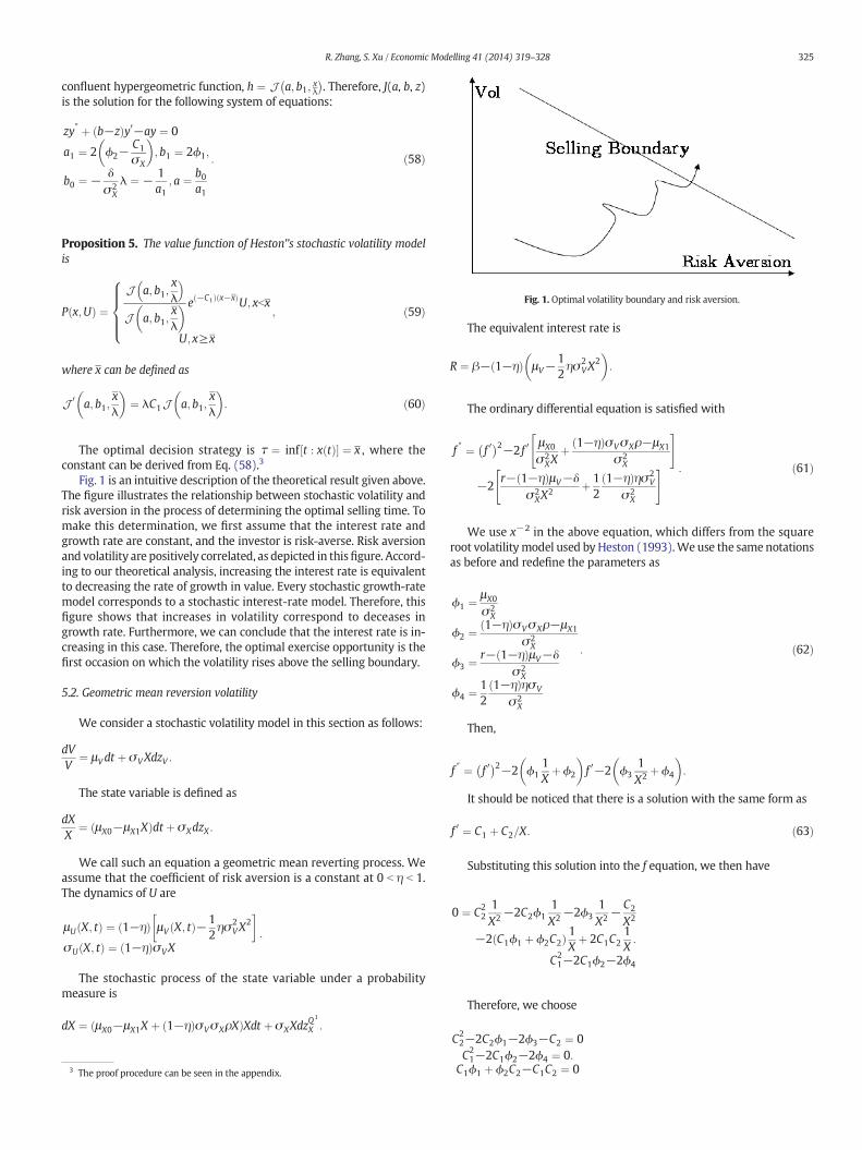
Fig. 1. Optimal volatility boundary and risk aversion.

325R. Zhang, S. Xu / Economic Modelling 41 (2014) 319–328

confluent hypergeometric function, h ¼ J a; b1; xλ� �

. Therefore, J(a, b, z)is the solution for the following system of equations:

zy″ þ b−zð Þy0−ay ¼ 0

a1 ¼ 2 ϕ2−C1

σX

� �; b1 ¼ 2ϕ1;

b0 ¼ − δσ2

X

λ ¼ − 1a1

; a ¼ b0a1

: ð58Þ

Proposition 5. The value function of Heston'’s stochastic volatility modelis

P x;Uð Þ ¼J a; b1;

xλ

�J a; b1;

xλ

� � e −C1ð Þ x−xð ÞU; xbx

U; x≥x

;

8>>><>>>:

ð59Þ

where x can be defined as

J 0 a; b1;xλ

� �¼ λC1J a; b1;

xλ

� �: ð60Þ

The optimal decision strategy is τ ¼ inf t : x tð Þ½ � ¼ x , where theconstant can be derived from Eq. (58).3

Fig. 1 is an intuitive description of the theoretical result given above.The figure illustrates the relationship between stochastic volatility andrisk aversion in the process of determining the optimal selling time. Tomake this determination, we first assume that the interest rate andgrowth rate are constant, and the investor is risk-averse. Risk aversionand volatility are positively correlated, as depicted in thisfigure. Accord-ing to our theoretical analysis, increasing the interest rate is equivalentto decreasing the rate of growth in value. Every stochastic growth-ratemodel corresponds to a stochastic interest-rate model. Therefore, thisfigure shows that increases in volatility correspond to deceases ingrowth rate. Furthermore, we can conclude that the interest rate is in-creasing in this case. Therefore, the optimal exercise opportunity is thefirst occasion on which the volatility rises above the selling boundary.

5.2. Geometric mean reversion volatility

We consider a stochastic volatility model in this section as follows:

dVV

¼ μVdt þ σVXdzV :

The state variable is defined as

dXX

¼ μX0−μX1Xð Þdt þ σXdzX :

We call such an equation a geometric mean reverting process. Weassume that the coefficient of risk aversion is a constant at 0 b η b 1.The dynamics of U are

μU X; tð Þ ¼ 1−ηð Þ μV X; tð Þ−12ησ2

VX2

� �σU X; tð Þ ¼ 1−ηð ÞσVX

:

The stochastic process of the state variable under a probabilitymeasure is

dX ¼ μX0−μX1X þ 1−ηð ÞσVσXρXð ÞXdt þ σXXdzQ1

X :

3 The proof procedure can be seen in the appendix.

The equivalent interest rate is

R ¼ β− 1−ηð Þ μV−12ησ2

VX2

� �:

The ordinary differential equation is satisfied with

f ″ ¼ f 0� �2−2 f 0

μX0

σ2XX

þ 1−ηð ÞσVσXρ−μX1

σ2X

" #

−2r− 1−ηð ÞμV−δ

σ2XX

2 þ 12

1−ηð Þησ2V

σ2X

" # : ð61Þ

We use x−2 in the above equation, which differs from the squareroot volatilitymodel used by Heston (1993).We use the samenotationsas before and redefine the parameters as

ϕ1 ¼ μX0

σ2X

ϕ2 ¼ 1−ηð ÞσVσXρ−μX1

σ2X

ϕ3 ¼ r− 1−ηð ÞμV−δσ2

X

ϕ4 ¼ 12

1−ηð ÞησV

σ2X

: ð62Þ

Then,

f ″ ¼ f 0� �2−2 ϕ1

1Xþ ϕ2

� �f 0−2 ϕ3

1X2 þ ϕ4

� �:

It should be noticed that there is a solution with the same form as

f 0 ¼ C1 þ C2=X: ð63Þ

Substituting this solution into the f equation, we then have

0 ¼ C221X2 −2C2ϕ1

1X2 −2ϕ3

1X2 −

C2

X2

−2 C1ϕ1 þ ϕ2C2ð Þ 1Xþ 2C1C2

1X:

C21−2C1ϕ2−2ϕ4

Therefore, we choose

C22−2C2ϕ1−2ϕ3−C2 ¼ 0C21−2C1ϕ2−2ϕ4 ¼ 0:

C1ϕ1 þ ϕ2C2−C1C2 ¼ 0

326 R. Zhang, S. Xu / Economic Modelling 41 (2014) 319–328

This set of equations can be solved to produce

C1 ¼ ϕ2 �ffiffiffiffiffiffiffiffiffiffiffiffiffiffiffiffiffiffiffiffiϕ22 þ 2ϕ4

qC2 ¼ C1ϕ1

C1−ϕ2

ϕ3 ¼ C22−2C2ϕ1−C2

2

:

Integrating both sides into Eq. (63), we can get

f ¼ C1X þ C2 lnX:

The e index is

ef ¼ XC2eC1X :

The discount rate δ can be determined by Eq. (62). The dynamics ofstate variable under probability Q2 is therefore

dXX

¼ μX0−σ2XC2 þ 1−ηð ÞσVσXρ−μX1−σ2

XC1

�X

h idt þ σXdz

Q2

X :

Then, according to Theorem 1, the asset value satisfies the followingequation:

12σ2

XX2h00 þ μX0−σ2

XC2 þ 1−ηð ÞσVσXρ−μX1−σ2XC1

�X

h iXh0−δh ¼ 0:

We rewrite this equation in a standard form as

a2X2h00 þ a1X

2 þ b1X �

h0 þ c0h ¼ 0:

All the constants are defined as follows:

a2 ¼ 12σ2

X

a1 ¼ 1−ηð ÞσVσXρ−μX1−σ2XC1:

b1 ¼ μX0−σ2XC2

c0 ¼ −δ

Let θ be the root of algebra equation

a2θ2 þ b1−a2ð Þθþ c0 ¼ 0:

The function Xθω(X) can be identified by solving the followingequation:

a2Xw00 þ a1X þ 2a2θþ b1ð Þh0 þ a1θh ¼ 0:

This is a Kummer equation that can be solved by themethod given inthe appendix. We choose a general solution CXθw(X) with boundaryconditions as follows:

CXθw Xð Þ ¼ XC2eC1X

Xθw0 Xð Þ þ θXθ−1w Xð Þ ¼ C1 þ C2=Xð ÞXC2eC1X:

By solving the above equations, we can get the constant

C ¼ XC2−θeC1X=w X� �

:

Proposition 6. The value function in a geometric mean reversionvolatility model is

P x;Uð Þ ¼X

X

� �θ−C2 w Xð Þw X� � eC1X

eC1XU; xbx

U; x≥x

:

8><>: ð64Þ

In this function, X is defined as

w0 X� �

w X� � ¼ C1 þ

C2−θX

: ð65Þ

In that case the optimal strategy is τ ¼ inf t : x tð Þ ¼ x½ �.The proof procedure can be seen in the appendix.

6. Conclusion

Unlike traditional stock selling-time theory, which usually as-sumes geometric Brownian motion, we introduce the considerationof stochastic volatility into the optimal selling-time model. Wemake the assumption of an incomplete market having CRRA inves-tors in a scale-invariant asset value growth process that is dependenton a stochastic state variable. Our method can be used to predict theexpected return and volatility in imperfectly correlated cases. Thiscapability allows investors to use more information sources, suchas the implied volatility inferred from derivative prices in a maturederivatives market. We prove that a path-dependent optimal invest-ment stopping problem can be transformed into a path-independentproblem. We work out explicit solutions for several special cases,such as situations of Heston stochastic volatility or Vasicek stochasticvolatility. The application of this method is not limited to the field ofoptimal investment, but also applies more generally to an optimalstopping framework.

Our paper makes several contributions to the empirical methodsof market analysis. We demonstrate how to transform a path-dependent stopping problem into a path-independent problemunder general conditions. This transformation method can be ap-plied to the settings of other path-dependent optimal stopping prob-lems. For example, stochastic volatility and stochastic risk premiumscould lead to path-dependent pricing models. For such situations,this paper provides one possible approach to solve the optimal stop-ping times problems.

Our analysis also has several empirical implications for the invest-ment industry. For example, we demonstrate that stock returns arechanging yet predictable to some extent, and that volatility is bothtime varying and persistent. Industry analysts can gain more excessreturn by exploiting this predictability. This paper extends research onthe optimal investment stopping issue to stochastic investment oppor-tunity environments. Our proposed method enhances the descrip-tive capability of optimal investment stopping theory in relationto the real capital market. In an efficient market, we suggest that in-vestors deduce information on basic assets from their derivativeprices.

This paper puts forward a method for investors to use in evaluatingtheir investment stopping decisions. Our analysis suggests that optimalstrategy and asset pricing may be seriously distorted due to investorignorance concerning return predictability. Buffet and Graham's basicinvestment principle concerns buying and holding until the assetreaches a certain pre-set condition to trigger trading. Our paper, how-ever, can serve as a means for a more rational analysis of value thatcan inform choices of timing.

As a possible application, we also investigate the economic impli-cations of our results on the disposition effect in the stock market.Our results show that there is at least one way to reach asymmetryin stock selling. Stochastic volatility can affect the selling time for

327R. Zhang, S. Xu / Economic Modelling 41 (2014) 319–328

risk-averse investors. If changes in volatility are negatively correlat-ed with changes in return, the volatility is more likely to decreasewhen the stock price increases. When investors are close to theirselling boundaries, they tend to sell more quickly. Otherwise, volatil-ity is more likely to increase when the stock price decreases. Wheninvestors are far from their selling boundaries, they tend to postponeselling.Wewill provide amore concise and detailed interpretation inour future research.

Acknowledgements

We would like to thank Stephen George Hall (the editor) andan anonymous referee for their helpful comments and suggestions.Ran Zhang thanks the financial support of National Natural ScienceFoundation of China (Grant No. 71003005 and 71373002).

Appendix A

A.1. Proof of Proposition 1

Based on Eq. (19), we can have

12p00σ2

XX3 þ μX þ σXσVρð ÞX2p0−μVXp ¼ 0:

After rearranging, we get the following homogeneous equation,

12p00σ2

XX2 þ μX þ σXσVρð ÞXp0−μVp ¼ 0:

Its solution is

v Xð Þ ¼ C−Xθ− þ CþXθþ

where θ is the solution of the following arithmetic equation,

12σ2

Xθ2 þ μX þ σXσVρ−

12σ2

X

� �θ−R1 ¼ 0:

We can get a positive solution and a negative solution if μV N 0 isheld. They are

θ� ¼− μX þ σXσVρ−

12σ2

X

� ��

ffiffiffiffiffiffiffiffiffiffiffiffiffiffiffiffiffiffiffiffiffiffiffiffiffiffiffiffiffiffiffiffiffiffiffiffiffiffiffiffiffiffiffiffiffiffiffiffiffiffiffiffiffiffiffiffiffiffiffiffiffiffiffiffiffiffiffiμX þ σXσVρ− 1

2σ2X

� �2 þ 2σ2XR1

qσ2

X

:

Because of A N 0,we expect that v is an increasing function of X. ThenC− = 0, v Xð Þ ¼ CþXθþ . Boundary conditions are

CþXθþ ¼ eAX ;

CþθþXθþ−1 ¼ AeAX :

From these two equations, we can obtain Cþ ¼ eAXX−θþ and X ¼ θþ

A .

A.2. Proof for Theorem 1

Use transformation p = he−f, the derivatives are

p0 ¼ h0− f 0h� �

ef;p″ ¼ h″−2 f 0h0− f ″hþ f 0

� �2hh ief:

Replace these into the pricing equation and rearrange it, we get

12σ2

Xh″ þ μX−σ2

X f0 �h0

þ 12σ2

X f 0� �2−1

2σ2

X f″−μX f

0−R� �

h ¼ 0: ðA:1Þ

To get a constant discount rate δ, we need to let the coefficient of hequal to δ. So we get the ordinary differential equation in Eq. (31).Under these conditions, the boundary conditions change into

h xð Þe− f xð Þ ¼ 1;h0 xð Þ− f 0 xð Þh xð Þ ¼ 0:

A.3. Proof for Theorem 2

A sufficient condition of Eq. (43) is

exp½−Z τ

0R Xð Þds� ¼ M2 τð Þ exp −δτð Þ exp f Xð Þ½ �:

We write M2 as

M2 ¼ exp −Z τ

0R Xð Þdsþ δτ− f Xð Þ

� �;

where M2(0) = 1. We can get the following equation by applying Ito'slemma to log M2,

dM2

M2¼ 1

2df Xð Þ½ �2−R Xð Þdt þ δdt−df Xð Þ:

After applying Ito's lemma to f, we get df= (fXμX + 0.5fXXσX2)dt+ f-

XσXdzX. Replace df into dM2, we get

EdM2

M2¼ 1

2f XσXð Þ2dt−R Xð Þdt þ δdt− f XμX þ 1

2f XXσ

2X

� �dt:

For keepingmartingale character ofM2, we should let drift equals tozero, that is, EdM2 = 0. After rearranging

12f XXσ

2X−

12

f XσXð Þ2 þ f XμX þ R Xð Þ−δ ¼ 0:

A.4. Proof for Proposition 5

The second order differential equation is

a2xþ b1ð Þy″ þ a1xþ b1ð Þy0 þ a0xþ b0ð Þy ¼ 0:

According to the handbook of exact solutions for ordinary dif-ferential equations (Polianin, 2002, page: 248), let J a; b; zð Þbe the solu-tion of following equation,

xy}þ b−xð Þy0−ay ¼ 0: ðA:2Þ

Case 1. a2 ≠ 0. That is, xy " + (a1x + b1)y ' + (a0x + b0)y = 0.The solution can be written as

y ¼ ekxJ a; b1; zð Þ: ðA:3ÞWhere,

z ¼ xλ; k ¼

ffiffiffiffiD

p−a12

;λ ¼ −12κ þ a1

; a ¼ B kð Þ2kþ a1

;D ¼ a21−4a0;B kð Þ¼ b1kþ b0:

Case 2. a2 = 0. That is, b2y " + (a1x + b1)y ' + b0y = 0.The solution can be written as

y zð Þ ¼ J a;12;βz2

� �: ðA:4Þ

Where,

z ¼ xþ b1a1

; a ¼ b02a1

;β ¼ − a12b2

:

Solution y = ekxw(z), where z ¼ x−μλ , D = a1

2 − 4a0a2, B(k) = b2k2 + b1k + b0.

Table 1

328 R. Zhang, S. Xu / Economic Modelling 41 (2014) 319–328

Constraints

k λ μ ω Parameters

a2≠0; a21≠4a0a2

ffiffiffiD

p−a1

2a2a

− a22a2kþa1

− b2a2

J(a, b; z)� �

a ¼ B kð Þ= 2a2kþ a1ð Þ; b ¼ a2b1−a1b2ð Þa−22

a2 ¼ 0; a1≠0

− 0a1

1

− 2b2kþb1a1

J a; 12 ;βz2

a ¼ B kð Þ= 2a1ð Þ;β ¼ −a1= 2b2ð Þ

a2≠0; a21 ¼ 4a0a2

− a12a2b

a2

− b2a2

2

zv=2Zv βffiffiffiz

p� �

v ¼ 1− 2b2kþ b1ð Þa−1

2 ;β ¼ 2ffiffiffiffiffiffiffiffiffiB kð Þ

p

a2 ¼ a1 ¼ 0; a21 ¼ 4a2a2 − 1

2b2

1 b1−4b0b2

4a0b2

z1/2Z1/3(βz3/2) β ¼ 2

3a0b2

�1=2

References

Alvarez, L.H.R., 2001. Reward Functionals. Salvage Values, and Optimal Stopping, Mathe-matical Methods of Operations Research 54, 315–337.

Alvarez, L.H.R., 2003. Stochastic forest growth and Faustmann's formula. J. Control. Optim.42, 1972–1993.

Alvarez, L.H.R., Koskela, E., 2004. Irreversible investment under interest rate variability:new results. Working paper.

Bekaert, G., Hodrick, Robert J., 1993. On biases in the measurement of foreign exchangerisk premiums. J. Int. Money Financ. 12 (2), 115–138.

Bensoussan, A., 1982. Stochastic Control by Functional Analysis Methods, (NorthHolland).

Bensoussan, A., Lions, J.L., 1982. Applications of Variational Inequalities in Stochastic Con-trol. North Holland, Amsterdam.

Black, F., Scholes, M., 1973. The pricing of options and corporate liabilities. J. Polit. Econ. 81(3), 637–654.

Brennan, Michael J., Xia, Y., 2000. Stochastic interest rates and bond-stock mix. Eur. Fi-nance Rev. 4 (2), 197–210.

Brennan, Michael J., Xia, Y., 2001. Dynamic asset allocation under inflation. J. Financ. 57(3), 1201–1238.

Brennan, Michael J., Xia, Y., 2002. Optimal investment policies: fixed mix and dynamicstochastic control models. Working paper UCLA.

Brock, W.A., Rothschild, M., Stiglitz, J.E., 1988. Stochastic capital theory. In: Feiwal, G. (Ed.),Essays in Honor of Joan Robinson'. Cambridge Univ. Press, Cambridge, UK.

Campbell, John Y., Shiller, Robert J., 1988. Stock prices, earnings and expected dividends.J. Financ. 43 (3), 661–676.

Campbell, John Y., Viceira, Luis M., 2002. Strategic Asset Allocation: Portfolio Choice forLong-Term Investors, (Oxford).

Dixit, A.K., Pindyck, R.S., 1994. Investment Under Uncertainty. Princeton University Press.Elliott, C.M., Ockendon, J.R., 1982. Weak and Variational Methods for Free and Moving

Boundary Problems. Pitman, London.Fama, Eugene F., French, Kenneth R., 1989. Business conditions and expected returns on

stocks and bonds. J. Financ. Econ. 25 (1), 23–49.Ferson,Wayne, Harvey, Campbell R., 1993. The Risk and Predictability of International Eq-

uity Returns. Rev. Financ. Stud. 6, 527–566.

Friedman, A., 1988. Variational Principles and Free Boundary Problems. Robert E. Krieger,Melbourne.

Goran, P., Shiryaev, A., 2006. Optimal Stopping and Free-Boundary Problems. Publisher:Birkhhauser, Basel 3764324198.

Grenadier, Steven R., Wang, N., 2005. Investment Timing. Agency and Information, J.Financ. Econ. 75, 493–533.

Henderson, V., 2002. Valuation of claims on non-traded assets using utility maximization.Math. Financ. 12 (4), 351–373.

Heston, Steven L., 1993. A closed-form solution for options with stochastic volatility withapplications to bond and currency options. Rev. Financ. Stud. 6 (2), 327–343.

Keim, Donald B., Stambaugh, Robert F., 1986. Predicting returns in the stock and bondmarkets. J. Financ. Econ. 17 (2), 357–390.

Kinderlehrer, D., Stampacchia, G., 1980. An Introduction to Variational Inequalities andtheir Applications. Academic Press, New York,.

Liang, X., Peng, X., Guo, J., 2014. Optimal investment, consumption and timing of annuitypurchase under a preference change. J. Math. Anal. Appl. 413, 905–938.

McDonald, R., Siegel, D., 1986. The value of waiting to invest. Q. J. Econ. 101, 707–728.Merton, R.C., 1973. Theory of rational option pricing. Bell J. Econ. Manag. Sci. 4 (1),

141–183.Miao, J., Wang, N., 2007. Investment, consumption, and hedging under incomplete mar-

kets. J. Financ. Econ. 86 (3), 608–642.Nishide, K., Nomi, E.K., 2009. Regime uncertainty and optimal investment timing. J. Econ.

Dyn. Control. 33, 1796–1807.Polianin, A.D., 2002. Handbook of Exact Solutions for Ordinary Differential Equations.

Second Edition, Chapman & Hall/CRC.Rishel, R., Kurt, H., 2006. A variational inequality sufficient condition for optimal stopping

with application to an optimal stock selling problemJ. Control. Optim. 45 (2),580–598.

Shibata, T., Nishihara, M., 2012. Investment timing under debt issuance constraint. J. Bank.Financ. 36, 981–991.

Wong, K.P., 2010. The effects of irreversibility on the timing and intensity of lumpy invest-ment. Econ. Model. 27, 97–102.

Wong, K.P., Yi, L., 2013. Irreversibility, mean reversion, and investment timing. Econ.Model. 30, 770–775.