Optimal sustainable harvesting of populations in random

Please cite this article as: L.H.R. Alvarez E. and A. Hening, Optimal sustainable harvesting of populations in random environments,Stochastic Processes and their Applications (2019), https://doi.org/10.1016/j.spa.2019.02.008.

Available online at www.sciencedirect.com

ScienceDirect

Stochastic Processes and their Applications xxx (xxxx) xxxwww.elsevier.com/locate/spa

Optimal sustainable harvesting of populations in randomenvironments

Luis H.R. Alvarez E.a, Alexandru Heningb,∗

a Department of Accounting and Finance, Turku School of Economics, FIN-20014 University of Turku, Finlandb Department of Mathematics, Tufts University, Bromfield-Pearson Hall, 503 Boston

Avenue, Medford, MA 02155, United States

Received 16 July 2018; received in revised form 18 December 2018; accepted 14 February 2019Available online xxxx

Abstract

We study the optimal sustainable harvesting of a population that lives in a random environment. Thenovelty of our setting is that we maximize the asymptotic harvesting yield, both in an expected value andalmost sure sense, for a large class of harvesting strategies and unstructured population models. We proveunder relatively weak assumptions that there exists a unique optimal harvesting strategy characterizedby an optimal threshold below which the population is maintained at all times by utilizing a local timepush-type policy. We also discuss, through Abelian limits, how our results are related to the optimalharvesting strategies when one maximizes the expected cumulative present value of the harvesting yieldand establish a simple connection and ordering between the values and optimal boundaries. Finally,we explicitly characterize the optimal harvesting strategies in two different cases, one of which is thecelebrated stochastic Verhulst Pearl logistic model of population growth.c⃝ 2019 Elsevier B.V. All rights reserved.

MSC: 92D25; 60J70; 60J60

Keywords: Ergodic control; Stochastic harvesting; Ergodicity; Stochastic logistic model; Stochastic environment

1. Introduction

When trying to establish the best harvesting policy of a certain species, one needs to takeinto account both the biological and economic implications. It is well known that overharvestingmight lead to the extinction of whole populations (see [8,12,25,29]). Many species of animals(birds, mammals, and fish) are endangered because of unrestricted harvesting or hunting. In

∗ Corresponding author.E-mail addresses: [email protected] (L.H.R. Alvarez E.), [email protected] (A. Hening).

https://doi.org/10.1016/j.spa.2019.02.0080304-4149/ c⃝ 2019 Elsevier B.V. All rights reserved.

http://www.elsevier.com/locate/spa

https://doi.org/10.1016/j.spa.2019.02.008

http://www.elsevier.com/locate/spa

mailto:[email protected]

mailto:[email protected]

https://doi.org/10.1016/j.spa.2019.02.008


2 L.H.R. Alvarez E. and A. Hening / Stochastic Processes and their Applications xxx (xxxx) xxx

some instances people have overestimated the population density of a certain species, and sinceit takes a while for a harvested population to recover to previous levels, this has led to eitherlocal or global extinctions. However, if we underharvest a species, this can lead to the lossof valuable resources. We are therefore presented with a conundrum: should we overharvestand gain economically but possibly drive a species extinct or should we underharvest to makesure extinction is less likely but lose precious resources? We present a model and a harvestingmethod which give us, based on a rigorous mathematical analysis, the best possible sustainableharvesting policy that does not drive the species extinct.

We study a population whose dynamics is continuous in time and that is affected by bothbiotic (competition) and abiotic (rainfall, temperature, resource availability) factors. Since theabiotic factors are affected by random disturbances, we look at a model that has environmentalstochasticity. This transforms a system that is modeled by an ordinary differential equation(ODE) into a system that is modeled by a stochastic differential equation (SDE). We refer thereader to [34] for a thorough discussion of environmental stochasticity.

We build on the results from [2,5] and [17]. Suppose that in an infinitesimal time dt weharvest a quantity d Z t where (Z t )t≥0 is any adapted, non-negative, non-decreasing, and rightcontinuous process. We determine the optimal harvesting strategy maximizing the expectedaverage asymptotic yield

ℓ = lim infT →∞

Ex1T

∫ T

0d Z t = lim inf

T →∞

Ex ZT

Tof harvested individuals. As in [17], and in contrast to what happens in a significant part ofthe literature (see [5,24–26]), the optimal strategy will be such that the population is neverdepleted and cannot be harvested to extinction. This is clear since if ZT → 0 in some sensethen ℓ = 0 in the above equation. Our main result is that the optimal harvesting strategy is ofthe local time reflection type: the population is kept in the interval (0, b∗] at all times by firstharvesting (x−b∗)+ and then harvesting only when the population hits the boundary just enoughto maintain the population density below b∗. This result was conjectured in [17] where theauthors showed that if the harvesting rate is bounded the optimal strategy is of bang–bang typei.e. there is a threshold x∗ > 0 such that if the population size is under x∗ there is no harvestingwhile if the population size is above x∗ we harvest according to the maximal rate M > 0. Ifone works with discounted yields like in [5], then interestingly the optimal harvesting strategyis also of this local time reflection type. In our setting the diffusion governing the unharvestedpopulation is much more general than the one from [5] and [17] where the authors mostlywork with a stochastic Verhulst–Pearl diffusion or its generalization. In the current paper wepresent a unifying result that encompasses a large variety of stochastic models.

Another advantage of our framework is that it does not depend on parameters that are hard tobe quantified empirically. Many papers from the literature (see [5]) work with a time discountedyield in order to capture the opportunity cost of capital. However, it is a difficult question tocome up with a good value for the discount factors (see [9]). Moreover, as [24] state in theirinfluential paper focusing on the relationship between discounting and extinction risk:

“Thus, even when the discount rate is less than the critical value predicted by determin-istic models, the economically optimal strategy will often be immediate harvesting toextinction. These results make a powerful argument that, for the common good, economicdiscounting should be avoided in the development of optimal strategies for sustainableuse of biological resources”.

Our model does not involve any discount factors. We generalize the setting of [17] where theauthors assumed the harvesting rate was bounded by some parameter M > 0. This corresponds


L.H.R. Alvarez E. and A. Hening / Stochastic Processes and their Applications xxx (xxxx) xxx 3

to having total control over the harvested population. Moreover, it also side-steps the need toknow the parameter M > 0 which could be hard to estimate realistically.

The paper is organized as follows. In Section 2 we introduce the model and prove the mainresults. Section 3 showcases how our model relates to the discounted model from [2,5]. Inparticular we show that by letting the discount rate go to zero, r ↓ 0, we can recover in asense the results of this paper. In Section 4 we look at two explicit applications of our results.As a first application we look at the Verhulst–Pearl diffusion model studied in [5,17]. Thesecond model we analyze is the one studied in [1,26]. Finally, Section 5 is dedicated to adiscussion of our results.

2. Model and results

We consider a population whose density X t at time t ≥ 0 follows, in the absence ofharvesting, the stochastic differential equation (SDE)

d X t = X tµ(X t ) dt + σ (X t ) d Bt , (1)

where (Bt )t≥0 is a standard one dimensional Brownian motion. This describes a population Xwith per-capita growth rate given by µ(x) > 0 and infinitesimal variance of fluctuations in theper-capita growth rate given by σ 2(x)/x2 when the density is X t = x . We make the followingstanding assumption throughout the paper.

Assumption 2.1. The functions µ, σ : (0,∞) → R are continuous and satisfy theEngelbert–Schmidt conditions:

σ (x) > 0 and ∃ε > 0 s.t.∫ x+ε

x−ε

1 + |yµ(y)|σ 2(y)

dy < ∞ for any x ∈ (0,∞).

These conditions ensure the existence and uniqueness of weak solutions to (1) (see forexample [10]). In addition, we want the population to persist in the absence of harvesting andto not explode to infinity (which would be absurd from a biological point of view). To this end,we will assume throughout our analysis that the boundaries of the state space of the populationdensity are unattainable (i.e. either natural or entrance) for X in the absence of harvesting. Thismeans that even though the process may tend towards a boundary, it will never attain it in finitetime. We refer the reader to Section 2.6 from [7] for a thorough discussion of the boundaryclassification of one-dimensional diffusions.

We denote the density of the scale function of X by

S′(x) = exp(

−

∫ x

c

2µ(y)yσ 2(y)

dy), (2)

where c ∈ R+ is an arbitrary constant. The density of the speed measure m is, in turn, denotedby

m ′(x) =2

σ 2(x)S′(x). (3)

We also set S((x, y)) =∫ y

x S′(t)dt and m((x, y)) =∫ y

x m ′(t)dt . The second order differentialoperator

A :=12σ 2(x)

d2

dx2 + µ(x)xd

dx=

12

ddm

dd S

(4)

is the infinitesimal generator of the underlying diffusion X .



For most harvesting applications it is sufficient to make the following assumption.

Assumption 2.2.

(A1) The function µ is nonincreasing and fulfills the limiting conditions limx→0+ µ(x) > η

and limx→∞ µ(x) < −η for some η > 0.(A2) The function µ(x)x has a unique maximum point x = argmax{µ(x)x} so that µ(x)x is

increasing on (0, x) and decreasing on (x,∞).(A3) limx→0+ m((x, y)) < ∞ for x < y.

Remark 2.1. It is worth pointing out that assumption (A1) guarantees that the per-capitagrowth rate µ vanishes at some given point x0 = µ−1(0). In typical population models thispoint coincides with the carrying capacity of the population. We naturally have that x < x0.

Condition (A3) is needed for the existence of a stationary distribution for the process X .Under our boundary assumptions, it guarantees that 0 is nonattracting for X and the conditionlimx→0+ S′(x) = +∞ is satisfied (cf. p. 234 in [23]).

A stochastic process (Z t )t≥0 taking values in [0,∞) is said to be an admissible harvestingstrategy if (Z t )t≥0 is non-negative, nondecreasing, right continuous, and adapted to the filtration(Ft )t≥0 generated by the driving Brownian motion (Bt )t≥0. We denote the class of all admissibleharvesting strategies (or controls) by Λ. Assume that (Z t )t≥0 ∈ Λ and that at time t we harvestin the infinitesimal period dt an amount d Z t . Then our harvested population’s dynamics isgiven up to the extinction date τ Z

0 = inf{t ≥ 0 : X Zt ≤ 0} by

d X Zt = X Z

t µ(X Zt ) dt + σ (X Z

t ) d Bt − d Z t , X Z0 = x > 0. (5)

As soon as the population becomes extinct we make the assumption that X Zt = 0 for all

t ≥ τ Z0 . However, as we will see below, these strategies will not be interesting since it will be

suboptimal to harvest the species to extinction.We consider the following ergodic singular control problem:

supZ∈Λ

lim infT →∞

1TEx

∫ T

0d Zs . (6)

We are interested (as in [17]) in the maximization of the expected asymptotic harvesting yield(also called the expected average cumulative yield) of the population.

Before presenting our main findings on the optimal ergodic harvesting strategy and the max-imal expected average cumulative yield we first establish the following auxiliary verificationlemma.

Lemma 2.1. Let ℓ be a given positive constant and assume that v : R+ ↦→ R+ is a twicecontinuously differentiable function satisfying the inequalities v′(x) ≥ 1 and (Av)(x) ≤ ℓ forall x ∈ R+. Then

lim infT →∞

1TEx

∫ T

0d Zs ≤ ℓ

for all Z ∈ Λ.



Proof. Applying the generalized Ito-Doblin (see [13]) change of variable formula to thenonnegative function v yields

v(X ZTn

) = v(x) +

∫ Tn

0(Av)(X Z

s )ds +

∫ Tn

0σ (X Z

s )v′(X Zs )d Bs

−

∫ Tn

0v′(X Z

s )d Zs +

∑s≤Tn

(v′(X Zs−)∆Zs + v(X Z

s ) − v(X Zs−)),

where T > 0 and Tn = T ∧ inf{t ≥ 0 : X Zt ∈ (1/n, n)} is an increasing sequence of finite

stopping times converging to T as n → ∞. The twice continuous differentiability of v impliesthat its derivative is bounded on (1/n, n) and since the harvesting policy has bounded variationwe notice that

0 ≤ v(X ZTn

) = v(x) +

∫ Tn

0(Av)(X Z

s )ds +

∫ Tn

0σ (X Z

s )v′(X Zs )d Bs

−

∫ Tn

0v′(X Z

s )d Z cs +

∑s≤Tn

(v(X Zs ) − v(X Z

s−)),

where Z c denotes the continuous part of an arbitrary admissible harvesting strategy Z ∈ Λ.Reordering terms and taking expectations shows that

Ex

∫ Tn

0v′(X Z

s )d Z cs + Ex

∑s≤Tn

∫ X Zs−

X Zs

v′(y)dy ≤ v(x) + Ex

∫ Tn

0(Av)(X Z

s )ds.

Imposing now the inequalities v′(x) ≥ 1 and (Av)(x) ≤ ℓ demonstrates that

Ex

∫ Tn

0d Zs ≤ v(x) + ℓEx Tn.

Letting n → ∞ and applying Fatou’s lemma together with the monotone convergence theoremyields

Ex

∫ T

0d Zs ≤ v(x) + ℓT

from which the alleged results follow. □

It is natural to ask if there is a function v and a constant ℓ∗ satisfying the conditions ofLemma 2.1. In order to show that the answer to this question is positive, we now follow theseminal paper [22] and investigate the following question: can we find two constants ℓ∗, b∗

and a twice continuously differentiable function u(x) satisfying the conditions

limx↓0

u′(x)S′(x)

= 0

(Au)(x) = ℓ∗, x ∈ (0, b∗),

u′(x) = 1, x ≥ b∗.

(7)

Using (4) we get

ddx

(u′(x)S′(x)

)= (Au)(x)m ′(x) = ℓ∗m ′(x), x ∈ (0, b∗).



The last equality, together with the boundary condition limx↓0 u′(x)/S′(x) = 0, yields that

u′(x) =

{ℓ∗S′(x)m((0, x)), if x ∈ (0, b∗)1 if x ≥ b∗

(8)

Invoking the twice continuous differentiability of u across the boundary b∗, and noting thatu′′(b∗) = 0 then shows that the constants ℓ∗, b∗ are the solutions of the system

ℓ∗= µ(b∗)b∗

=1

S′(b∗)m((0, b∗)). (9)

We can now establish the following.

Lemma 2.2. The optimality conditions (9) have a unique solution and for all Z ∈ Λ

lim infT →∞

1TEx

∫ T

0d Zs ≤ ℓ∗

= supb>0

{1

S′(b)m((0, b))

}=

1S′(b∗)m((0, b∗))

where b∗ is the unique zero of

f (x) =

∫ x

0(µ(y)y − µ(x)x)m ′(y)dy.

Furthermore, the function u defined by (7) satisfies the conditions of Lemma 2.1.

Proof. We first show that the optimality conditions (9) have a unique solution under ourassumptions. To this end we investigate the behavior of the continuous function f : (0,∞) →

R defined by

f (x) :=1

S′(x)− µ(x)xm((0, x)).

Making use of Assumption (A3) guarantees that∫ x

0µ(y)ym ′(y)dy =

∫ x

0

(1

S′(z)

)′

dz =1

S′(x)− lim

y→0+

1S′(y)

=1

S′(x).

Therefore, we can express f (x) as

f (x) =

∫ x

0(µ(y)y − µ(x)x)m ′(y)dy.

It is clear that f (x) < 0 and

f (x0) =

∫ x0

0µ(y)ym ′(y)dy > 0.

Therefore, using the intermediate value theorem, we conclude that f has at least one rootb∗

∈ (x, x0). To prove that the root is unique, we notice that if y > x , then

f (y) − f (x) =1

S′(y)− µ(y)ym((0, y)) −

(1

S′(x)− µ(x)xm((0, x))

)=

∫ y

xµ(t)tm ′(t)dt − µ(y)ym((0, y)) + µ(x)xm((0, x))

=

∫ y

x(µ(t)t − µ(y)y)m ′(t)dt + (µ(x)x − µ(y)y)m((0, x)).



Hence, if x < y ≤ x then f (y) − f (x) < 0 proving that f is strictly decreasing on (0, x).If, in turn, x ≤ x < y then f (y) − f (x) > 0 proving that f is strictly increasing on (x,∞).Combining these observations with the continuity of f and the fact that limx→0+ f (x) = 0then proves that the root b∗

∈ (x, x0) is unique and, consequently, that a unique pair ℓ∗, b∗

exists. Moreover, since

ddb

[1

S′(b)m((0, b))

]=

−2 f (b)σ 2(b)S′(b)m2((0, b))

we get that

b∗= argmax

{1

S′(b)m((0, b))

}and

ℓ∗=

1S′(b∗)m((0, b∗))

= µ(b∗)b∗.

We now prove that the function u satisfies the conditions of Lemma 2.1. We first observethat (Au)(x) = µ(x)x for all x ∈ [b∗,∞). Since µ(x)x is decreasing on (x,∞) and b∗ > xwe find that (Au)(x) ≤ ℓ∗

= µ(b∗)b∗ for all x ∈ R+. On the other hand, since

u′′(x) =2S′(x)ℓ∗

σ 2(x)

(1

S′(x)− µ(x)xm((0, x))

)=

2S′(x)ℓ∗

σ 2(x)f (x) < 0

for all x < b∗ and u′(b∗) = 1 we find that u′(x) ≥ 1 for all x ∈ R+. The last alleged claimnow follows from Lemma 2.1. □

Remark 2.2. Lemma 2.2 also shows that the function u(x) satisfying the considered freeboundary value problem is concave on R+. This property is later shown to be the principaldeterminant of the sign of the impact of increased volatility on the optimal harvesting policyand the expected average cumulative yield.

Lemma 2.2 essentially shows that if there is an admissible harvesting strategy satisfying thevariational inequalities of Lemma 2.1, then the value of that policy dominates the value of themaximal expected average cumulative yield. Naturally, if we could determine an admissiblepolicy yielding precisely the value characterized in Lemma 2.2, then that policy wouldautomatically constitute an optimal harvesting policy. This is accomplished in the followingtheorem summarizing our main result on the optimal sustainable harvesting policy.

Theorem 2.1. Suppose Assumptions 2.1 and 2.2 hold and X Z0 = x > 0. An optimal harvesting

strategy is

Zb∗

t =

{(x − b∗)+ if t = 0,(x − b∗)+ + L(t, b∗) if t > 0

(10)

where L(t, b∗) is the local time push of the process X Z at the boundary b∗ (cf. [13,22,32]).The optimal harvesting boundary b∗ as well as the maximal expected average asymptotic yieldℓ∗ are the solutions of the optimality conditions

ℓ∗= µ(b∗)b∗

=1

S′(b∗)m((0, b∗)).



Moreover,

supZ∈Λ

lim infT →∞

1TEx

∫ T

0d Zs = lim

T →∞

Ex [Zb∗

T ]T

= ℓ∗= µ(b∗)b∗.

Proof. It is clear that the proposed harvesting strategy Zb∗

is admissible. Our objective isnow to show that this policy attains the maximal expected average cumulative yield ℓ∗ andis, therefore, optimal. To show that this is indeed the case, we first notice that the harvestingpolicy Zb∗

is continuous on t > 0, increases only when X Zb∗

t = b∗, and maintains the processX Zb∗

t in (0, b∗] for all t > 0 [13,22,32]. In this case (5) can be re-expressed as

Zb∗

T = x − X Zb∗

T +

∫ T

0µ

(X Zb∗

t

)X Zb∗

t dt +

∫ T

0σ

(X Zb∗

t

)d Bt .

The continuity of the diffusion coefficient σ (x) now guarantees that σ (X Zb∗

t ) is bounded forall t > 0 and, therefore, that

Ex[Zb∗

T

]T

=

x − Ex

[X Zb∗

T

]T

+1TEx

∫ T

0µ

(X Zb∗

t

)X Zb∗

t dt.

Consequently,

limT →∞

Ex[Zb∗

T

]T

= limT →∞

1TEx

∫ T

0µ

(X Zb∗

t

)X Zb∗

t dt.

Since m((0, b∗)) < ∞ we notice that the process is ergodic and has an invariant probabilitymeasure π (·) =

m(·)m((0,b∗)) (cf. [7], pp. 37–38). Hence, since the function p(x) = xµ(x) is

bounded on [0, b∗] we have by pp. 37–38 [7] and the optimality condition (9)

limT →∞

1TEx

∫ T

0µ

(X Zb∗

t

)X Zb∗

t dt =

∫ b∗

0µ(x)x

m ′(x)m((0, b∗))

dx = µ(b∗)b∗= ℓ∗.

This demonstrates the optimality of the proposed policy. □

Remark 2.3. It is worth noticing that since (cf. pp. 36–38 in [7])

limt→∞

∫ t0 µ(Xs)Xs1(0,b](Xs)ds∫ t

0 1(0,b](Xs)ds=

1S′(b)m((0, b))

= µ(b)b

our findings are in line with observations based on renewal theoretic approaches to ergodiccontrol (cf. Chapter 5 in [13]). On the other hand we also observe that

b∗= argmax

b∈R+

{E

[µ(X Zb

∞)X Zb

∞

]}where X t denotes the population density in the absence of harvesting and X Zb

t → X Zb∞

∼

m ′(x)1(0,b](x)/m((0, b)) as t ↑ ∞. Consequently, the same conclusion could be obtained byfocusing on the ergodic limit of the process controlled by Zb

t .

Theorem 2.1 demonstrates that the optimal harvesting policy is of the standard local timepush type in the ergodic control setting as well. Consequently, under the optimal harvestingpolicy, the population is maintained below an optimal threshold by harvesting (in an infinitelyintense fashion) only at instants when the population hits the optimal boundary. Below thecritical threshold the population is naturally left unharvested.



It is at this point worth mentioning that a different approach to this problem could alsohave been possible. Namely, one could have tried to follow the approach developed in [35].However, the setting from [35] does not apply directly as the drift µ will not always be positive,the state space is (0,∞) instead of R, and we can have infx σ (x) = 0 (see Assumption 2.1from [35]).

One may wonder whether the findings of Theorem 2.1 could be extended further to a settingfocusing on the almost sure maximization problem

supZ∈Λ

lim infT →∞

1T

∫ T

0d Z t = sup

Z∈Λlim infT →∞

ZT

T. (11)

This is an almost sure statement, compared to the maximization from (6) which deals withexpected values. Related control problems have been analyzed in [6]. However, the particularsingular control problem we are interested in is not addressed in [6].

In order to delineate general circumstances under which the almost sure maximizationproblem admits a local time push type solution, we initially analyze the problem by focusingsolely on this type of harvesting policies. Our main findings on that class are established inthe next proposition.

Proposition 2.1. Let Zb∈ Λ be an arbitrary local time push type harvesting policy

maintaining the population density on (0, b) for all t > 0. Then, for any X Z0 = x ∈ (0, b)

Px

{lim

T →∞

ZbT

T= lim

T →∞

1T

∫ T

0µ

(X Zb

t

)X Zb

t dt =1

S′(b)m((0, b))

}= 1. (12)

Consequently,

Px

{lim

T →∞

ZbT

T≤ lim

T →∞

Zb∗

T

T= sup

b>0

{1

S′(b)m((0, b))

}= µ(b∗)b∗

}= 1. (13)

Proof. Let b ∈ (0,∞) be an arbitrary finite boundary and consider the policy Zbt ∈ Λ

maintaining the population density in (0, b) for all t > 0. As in the case of Theorem 2.1,the policy is continuous on t > 0 and increases only when X Zb

t = b. Moreover,

ZbT

T=

xT

+1T

∫ T

0µ

(X Zb

t

)X Zb

t dt +1T

∫ T

0σ

(X Zb

t

)d Bt −

X Zb

T

T. (14)

Since |X Zbt | ≤ b for all t > 0

limT →∞

X Zb

T

T= 0 (15)

with probability 1. Since m((0, b)) < ∞ the controlled process is ergodic on (0, b) and has aninvariant probability measure π (·) =

m(·)m((0,b)) . Invoking the ergodic results from [7] (pp. 37–38)

shows that almost surely

limT →∞

1T

∫ T

0µ

(X Zb

t

)X Zb

t dt =

∫ b

0µ(x)x

m ′(x)m((0, b))

dx =1

S′(b)m((0, b)). (16)



Let LT =∫ T

0 σ(

X Zbt

)d Bt . Then (LT )T ≥0 is a local martingale with quadratic variation

QT =∫ T

0 σ2(

X Zbt

)dt . By the ergodic results from [7], one has that almost surely

lim supT →∞

Qt

T=

∫ b

0σ 2(x)

m ′(x)m(0, b)

dx < ∞.

This combined with the Law of Large Numbers for local martingales (see Theorem 1.3.4from [28]) yields that almost surely

limT →∞

1T

∫ T

0σ

(X Zb

t

)d Bt = 0. (17)

Using (15), (16) and (17) in (14) we get that (12) holds almost surely. (13) then follows fromLemma 2.2. □

Proposition 2.1 shows that the local time push controls affect the dynamics of the controlledpopulation density in a way where the almost sure asymptotic average cumulative harvest canbe computed explicitly in terms of the exogenous harvesting boundary. Since this representationis valid for all local time push controls, we find that choosing the threshold according tothe rule maximizing the long run expected average cumulative harvest results in a maximalrepresentation in this setting as well. Given the generality of admissible harvesting strategies,it is a challenging task to prove a general verification lemma analogous to Lemma 2.1.Fortunately, there is a relatively large class of processes for which the desired result is valid.To see that this is indeed the case, we first establish the following auxiliary result.

Lemma 2.3. Assume (1) has a pathwise unique solution and there exists an increasingfunction ρ : R+ → R such that |σ (x) − σ (y)| ≤ ρ(|x − y|) for all x, y ∈ (0,∞) and∫

0+ρ−2(z) dz = +∞. Suppose X is the solution to (1) and X Z is the solution to (5) for a

fixed Z ∈ Λ. If X Z0 ≤ X0 then almost surely

P{X Zs ≤ Xs, s ≥ 0} = 1.

Proof. This is a modification of the arguments from the seminal papers [37] and [18]for the comparison of one-dimensional diffusions and the paper [38] for the comparison ofsemimartingales. For small ε > 0 define the process X ε via

d X εt = X ε

t (µ(X εt ) + ε) dt + σ (X ε

t ) d Bt .

Assume that X0 = X ε0. By [18] we see that almost surely

Xs ≤ X εs , s ≥ 0.

By the pathwise uniqueness of solutions of (1), combined with the continuity of µ we havealmost surely that

Xs = limε↓0

X εs , s ≥ 0.

We note that the semimartingales X Z and X ε satisfy the assumptions of Theorem 1 from [38].Therefore, if X Z

0 ≤ X ε0, we have that almost surely

X Zs ≤ X ε

s , s ≥ 0.



Taking the limit as ε ↓ 0 we get

X Zs ≤ Xs, s ≥ 0

which finishes the proof. □

Remark 2.4. We make two remarks on the assumptions needed in Lemma 2.3. First ofall, sufficient conditions for pathwise uniqueness of solutions can be found, for example,in [19,21,28]. Second, for most models of natural resources σ (x) = σ x for some σ > 0.In those cases the required growth condition is satisfied by simply taking ρ(x) = σ (x) = σ x .

Lemma 2.3 states a set of conditions under which the solution of the uncontrolled dynamics(1) dominates the solution of the dynamics subject to harvesting (5). It is worth pointingout that similar comparison results have been previously established for Lipschitz-continuouscoefficients (see Theorem 54 in [30]). However, that result does not directly apply to our setting,since most applied population models have only locally Lipschitz-continuous coefficients.Given our findings in Lemma 2.3 we can now establish the following Theorem which extendsour results on the expected average cumulative yield to the almost sure setting.

Theorem 2.2. Assume that Assumptions 2.1 and 2.2 hold, that (1) has pathwise uniquesolutions, that there exists an increasing function ρ : R+ → R such that |σ (x) − σ (y)| ≤

ρ(|x − y|) and∫

0+ρ−2(z) dz = +∞, and that

1. The process X from (1) has a unique invariant probability measure on (0,∞).2. One can find a twice continuously differentiable function v : R+ ↦→ R+ satisfying the

variational inequalities v′(x) ≥ 1 and (Av)(x) ≤ ℓ for all x ∈ R+.3. The function g(x) := σ (x)v′(x) is non-decreasing and square-integrable with respect to

the speed measure of X.

Then for any admissible strategy Z ∈ Λ and any X Z0 = x ∈ (0,∞)

Px

{lim infT →∞

ZT

T≤ ℓ

}= 1. (18)

Moreover,

Px

{lim infT →∞

ZT

T≤ lim inf

T →∞

Zb∗

T

T= ℓ∗

= µ(b∗)b∗

}= 1 (19)

for all Z ∈ Λ and all X Z0 = x ∈ (0,∞).

Proof. It is clear that for any admissible policy Z ∈ Λ we have

ZT

T≤v(x)

T+ ℓ+

1T

∫ T

0σ (X Z

s )v′(X Zs )d Bs . (20)

The local martingale

QT =

∫ T

0σ (X Z

s )v′(X Zs )d Bs

has quadratic variation

1T

[Q, Q]T =1T

∫ T

0(σ (X Z

s ))2(v′(X Zs ))2ds.



By our assumptions and Lemma 2.3 we have almost surely that

X Zs ≤ Xs, s ≥ 0.

Then, almost surely, because of assumption 3 of the theorem,

1T

[Q, Q]T =1T

∫ T

0(σ (X Z

s ))2(v′(X Zs ))2ds ≤

1T

∫ T

0(σ (Xs))2(v′(Xs))2ds.

By the ergodic results from [7] and the assumptions of the proposition, one has that almostsurely

lim supT →∞

1T

[Q, Q]T ≤ limT →∞

1T

∫ T

0(σ (Xs))2(v′(Xs))2ds

=

∫g(x)m ′(x)/m((0,∞))dx < ∞.

The Law of Large Numbers for local martingales (see Theorem 1.3.4 from [28]) yields thatalmost surely

limT →∞

QT

T= 0.

If we combine this with (20) we get

lim infT →∞

ZT

T≤ ℓ.

Finally, inequality (19) follows from (18) and (13). □

Remark 2.5. We make the following three remarks on the assumptions (1)–(3) needed inTheorem 2.2.

(a) If 0,∞ are unattainable and nonattracting, i.e. for any x ∈ (0,∞) we have Px {X t → 0} =

Px {X t → ∞} = 0, and m((0,∞)) < ∞ then X has a unique invariant probabilitymeasure with density m′(·)

m((0,∞)) on (0,∞). In terms of boundary behavior the points 0,∞can be entrance or natural, and the natural boundaries have to be nonattracting.

(b) We note that the function u defined in (7) satisfies (Au)(x) ≤ ℓ∗= µ(b∗)b∗ and

u′(x) ≥ 1, x ∈ R+.(c) Checking condition (6) reduces to looking at the function

g(x) = σ (x)u′(x) =

{σ (x)ℓ∗S′(x)m((0, x)), if x ∈ (0, b∗)σ (x) if x ≥ b∗,

(21)

verifying that it is non-decreasing, and then checking whether∫

∞

0 g2(x)m ′(x) dx < ∞.If σ (·) is continuously differentiable and nondecreasing and

12σ (x)σ ′(x)m((0, x)) +

∫ x

0(µ(t)t − µ(x)x)m ′(t)dt ≥ 0

for all x ∈ (0, b∗) then g(·) is nondecreasing

Remark 2.6. Our work is related to [20] where the authors consider the more general casewhere there are two controls. Consider the controlled diffusion

d X t = µ(X t ) dt + σ (X t ) d Bt + dξ+

t − dξ−

t



where ξ is a right-continuous process with left limits that has finite variation and is adapted.Fix a starting point X (0) = x ∈ R. The paper [20] is concerned with the minimization of

lim supT →∞

1TEx

[∫ T

0h(Xs) ds +

∫[0,T ]

k+(Xs)dξ+

s +

∫[0,T ]

k−(Xs)dξ−

s

]and the almost sure minimization of

lim supT →∞

1T

[∫ T

0h(Xs) ds +

∫[0,T ]

k+(Xs)dξ+

s +

∫[0,T ]

k−(Xs)dξ−

s

].

Here h : R → R is a given function that models the running cost resulting from the system’soperation, while k+, k− are given functions penalizing the expenditure of control effort. Wenote that one of their assumption is that 0 < σ 2(x) ≤ C(1 + |x |), which is more restrictivethan what we have since in most population models σ (x) = σ x .

Our main result on the sign of the relationship between volatility and the optimal harvestingstrategy is summarized in the following.

Theorem 2.3. Increased volatility increases the optimal harvesting threshold b∗ and decreasesthe long run average cumulative yield ℓ∗

= µ(b∗)b∗.

Proof. Denote by b the optimal harvesting threshold and by ℓ the maximal expected averagecumulative yield associated with the more volatile dynamics characterized by the diffusioncoefficient σ (x) ≥ σ (x) for all x ∈ R+ and let

A =12σ 2(x)

d2

dx2 + µ(x)xd

dxdenote the differential operator associated with the more volatile process. Let u(x) be thesolution of the free boundary problem (7). Because u′′(x) ≤ 0 we get

(Au)(x) =12

(σ 2(x) − σ 2(x))u′′(x) + (Au)(x) ≤ ℓ∗

for all x ∈ R+. Since we also have u′(x) ≥ 1 we notice by combining Theorem 2.1 andLemma 2.2 that ℓ ≤ ℓ∗. However, since ℓ = µ(b)b, ℓ∗

= µ(b∗)b∗, and the optimal harvestingthreshold is on the set where the drift is decreasing, we find b ≥ b∗ which completes the proofof our claim. □

3. Discounting and harvesting: Connecting the harvesting problems

The previous section focused on the optimal ergodic harvesting policy maximizing theexpected (or almost sure) long-run average cumulative yield. It is naturally of interest toanalyze in which way the optimal policy differs from the optimal policies suggested by modelsmaximizing the expected present value of the cumulative yield. To this end, let (cf. [2])

Vr (x) = supZ∈Λ

Ex

∫∞

0e−rsd Zs (22)

denote the value of the harvesting policy maximizing the expected present value of thecumulative yield. Our objective is to characterize how the different problems are connectedby relying on an Abelian limit result first developed within singular stochastic control in theseminal paper [22] (see also [36] for a generalization).



In order to present our main findings on the connection between the two different approacheswe first have to make a set of assumptions guaranteeing that the harvesting policy maximizingthe expected present value of the cumulative yield is nontrivial. Define the function θr : R ↦→ Rby

θr (x) = (µ(x) − r )x,

where r > 0 denotes the prevailing discount rate. In addition to our assumptions on theboundary behavior of the population dynamics stated in Section 2 we now assume thefollowing.

Assumption 3.1. The function θr (x) satisfies

(B1) limx↓0 θr (x) ≥ 0 and limx→∞ θr (x) < −ε, where ε > 0.(B2) the function θr (x) attains a unique maximum at xr ∈ (0, xr

0), where xr0 = inf{x > 0 :

θr (x) = 0}.

Remark 3.1. Note that if µ is continuous on [0,∞) then Assumptions 2.1 and 2.2 imply(B1) above.

As was established in [2], one gets

Vr (x) =

⎧⎪⎨⎪⎩x +

1rθr (x∗

r ), x ≥ x∗r ,

ψr (x)ψ ′

r (x∗r ), x < x∗

r .(23)

The quantity ψr (x) denotes the increasing fundamental solution of the differential equation(Au)(x) = ru(x). The optimal harvesting boundary x∗

r = argmin{ψ ′r (x)} ∈ (xr , x0) is

the unique root of the ordinary first order optimality condition ψ ′′r (x∗

r ) = 0 which can bere-expressed as∫ x∗

r

0ψr (z)(θr (t) − θr (x∗

r ))m ′(z)dz = 0. (24)

The value of the optimal harvesting policy Vr (x) is monotonically increasing, concave,and twice continuously differentiable. Moreover, increased volatility decreases the value ofthe optimal policy and expands the continuation region where harvesting is suboptimal byincreasing the optimal harvesting boundary x∗

r .Under the optimal harvesting policy Z∗ the population density converges in law to its unique

stationary distribution. In other words, X Z∗

t ⇒ Xr as t → ∞. The random variable Xr isdistributed on (0, x∗

r ) according to the density

P[Xr ∈ dy

]=

m ′(y)dym((0, x∗

r )).

We can now establish the following limiting result

Lemma 3.1. Under our assumptions, increased discounting decreases the maximal expectedpresent value of the cumulative yield and accelerates harvesting by decreasing the optimalharvesting boundary. Moreover, limr→0+ x∗

r = b∗ where b∗ is the optimal harvesting boundaryfrom Theorems 2.1 and 2.2.



Proof. The monotonicity of the admissible harvesting strategy guarantees that increaseddiscounting decreases the value of the optimal policy. To see that it also accelerates harvestingby decreasing the optimal harvesting boundary we first observe that under our assumptions theconditions of Lemma 3.1 in [3] are met and, therefore,

ψr (x) − xψ ′r (x)

S′(x)=

∫ x

0ψr (t)θr (t)m ′(t)dt (25)

for all x ∈ R+. Reordering terms shows that (25) can be re-expressed as

ur (x) :=ψr (x)ψ ′

r (x)− x =

S′(x)ψ ′

r (x)

∫ x

0ψr (t)θr (t)m ′(t)dt. (26)

On the other hand, if τy = inf{t ≥ 0 : X t = y} denotes the first hitting time to y, then theidentity (cf. p. 18 in [7])

Ex[e−rτy ; τy < ∞

]=ψr (x)ψr (y)

guarantees that if r > r then

ψr (x)ψr (y)

≥ψr (x)ψr (y)

for all 0 < x < y < ∞. Using the last inequality we note that if r > r then

ψr (x)ψr (y)

= exp(

−

∫ y

xd lnψr (t)

)= exp

(−

∫ y

x

ψ ′r (t)ψr (t)

dt)

≥ψr (x)ψr (y)

= exp(

−

∫ y

x

ψ ′

r (t)ψr (t)

dt)

for all 0 < x < y < ∞. This implies∫ y

x

ψ ′r (t)ψr (t)

dt ≤

∫ y

x

ψ ′

r (t)ψr (t)

dt

for all 0 < x < y < ∞. This, together with the continuity of the functions and their derivatives,shows that

ψ ′r (x)ψr (x)

≤ψ ′

r (x)ψr (x)

for all x > 0. Consequently, ur (x) ≤ ur (x) for all x ∈ R+. Since ur (x∗r ) = θr (x∗

r ) andθr (x) ≥ θr (x) for all x ∈ R+ we notice that

ur (x∗

r ) ≥ θr (x∗

r ) ≥ θr (x∗

r )

implying that∫ x∗r

0ψr (t)θr (t)m ′(t)dt ≥ θr (x∗

r )ψ ′

r (x∗r )

S′(x∗r )

and, therefore, that x∗

r ≤ x∗r . This shows that higher discounting accelerates harvesting by

decreasing the optimal threshold.It remains to consider the limiting case where r ↓ 0. To this end, consider the function

Fr (x) =

∫ x

0

ψr (z)ψr (x)

(θr (z) − θr (x))m ′(z)dz.



Since

Ez[e−rτx ; τx < ∞] =ψr (z)ψr (x)

for z ≤ x we notice by letting r ↓ 0 and invoking our assumptions that

limr↓0

ψr (z)ψr (x)

= Pz [τx < ∞] = 1.

Since limr↓0 θr (x) = µ(x) we finally notice that

limr↓0

Fr (x) =

∫ x

0(µ(z)z − µ(x)x)m ′(z)dz = f (x).

The alleged claim now follows from (24) and Lemma 2.2. □

According to Lemma 3.1 higher discounting accelerates harvesting and results into alower expected asymptotic population density. Interestingly, the optimal harvesting thresholdapproaches the one from the average cumulative yield setting as r → 0+. It is clear thatthe same conclusion is not directly valid for the value of the optimal policy Vr (x). However,there exists an Abelian limit connecting the value of the two seemingly different controlproblems [22,36]. This connection is established in the following.

Theorem 3.1. Under our assumptions,

limr→0+

r Vr (x) = µ(b∗)b∗= ℓ∗

for all x ∈ R+.

Proof. Utilizing the fact that r Vr (x∗r ) = µ(x∗

r )x∗r and reordering terms in (23) yields

r Vr (x) =

⎧⎪⎨⎪⎩µ(x∗

r )x∗r + r (x − x∗

r ), x ≥ x∗r ,

µ(x∗r )x∗

r − r∫ x∗

r

x

ψ ′r (t)

ψ ′r (x∗

r )dt, x < x∗

r .

Since ψ ′r (t)/ψ ′

r (x∗r ) ∈ [1, ψ ′

r (x)/ψ ′r (x∗

r )] for all t ∈ [x, x∗r ] we find by invoking the limiting

result of Lemma 3.1 and the continuity of µ that

limr→0+

r Vr (x) =

{µ(b∗)b∗, x ≥ x∗

r ,

µ(b∗)b∗, x < x∗r .

This completes the proof. □

4. Applications

4.1. Verhulst-Pearl diffusion

Assume that the unharvested population follows the standard Verhulst–Pearl diffusion

d X t = µX t (1 − γ X t )dt + σ X t dWt , X0 = x ∈ R+, (27)

where µ > 0 is the per-capita growth rate at low densities, 1/γ > 0 is the carrying capacity,and σ > 0 is the infinitesimal variance of fluctuations in the per-capita growth rate. In thiscase

S′(x) = x−2µσ2 e

2µγσ2 x



and

m ′(x) =2σ 2 x

2µσ2 −2e−

2µγσ2 x

.

Moreover, if µ > σ 2/2 is satisfied, then

m((0, x)) =2σ 2

(σ 2

2µγ

) 2µσ2 −1 (

Γ

(2µσ 2 − 1

)− Γ

(2µσ 2 − 1,

2µγ xσ 2

))where Γ (·) is the gamma function and Γ (·, ·) is the upper incomplete gamma function. Wenote that in this case Assumptions 2.1, 2.2 and the conditions of Theorem 2.2 hold (see [11]for a thorough investigation of (27)). Consequently,

ℓ∗=

12σ 2

γ

(σ 2

2µ

)1−2µσ2

argmax

⎧⎨⎩ (γ x)2µσ2 e−

2µγσ2 x

Γ(

2µσ 2 − 1

)− Γ

(2µσ 2 − 1, 2µγ x

σ 2

)⎫⎬⎭ .

The optimal boundary b∗ reads as b∗= ρ∗γ−1, where ρ∗ is the unique root of the equation(

2µρ∗

σ 2

)1−2µσ2

(1 − ρ∗)e2µρ∗

σ22µσ 2

(Γ

(2µσ 2 − 1

)− Γ

(2µσ 2 − 1,

2µρ∗

σ 2

))= 1.

This shows that the optimal harvesting boundary is directly proportional to the carryingcapacity.

As was shown in [5], in this case the harvesting boundary maximizing the expected presentvalue of the cumulative yield constitutes the root of the equation ψ ′′

r (x∗r ) = 0, where r > 0

denotes the prevailing discount rate,

ψr (x) = (γ x)α1 M(α1, 1 + α1 − α2,

2µγ xσ 2

),

M denotes the Kummer confluent hypergeometric function,

α1 :=12

−µ

σ 2 +

√(12

−µ

σ 2

)2

+2rσ 2 > 0,

and

α2 :=12

−µ

σ 2 −

√(12

−µ

σ 2

)2

+2rσ 2 < 0.

We notice again that as in the ergodic setting, the optimal threshold is directly proportional tothe carrying capacity.

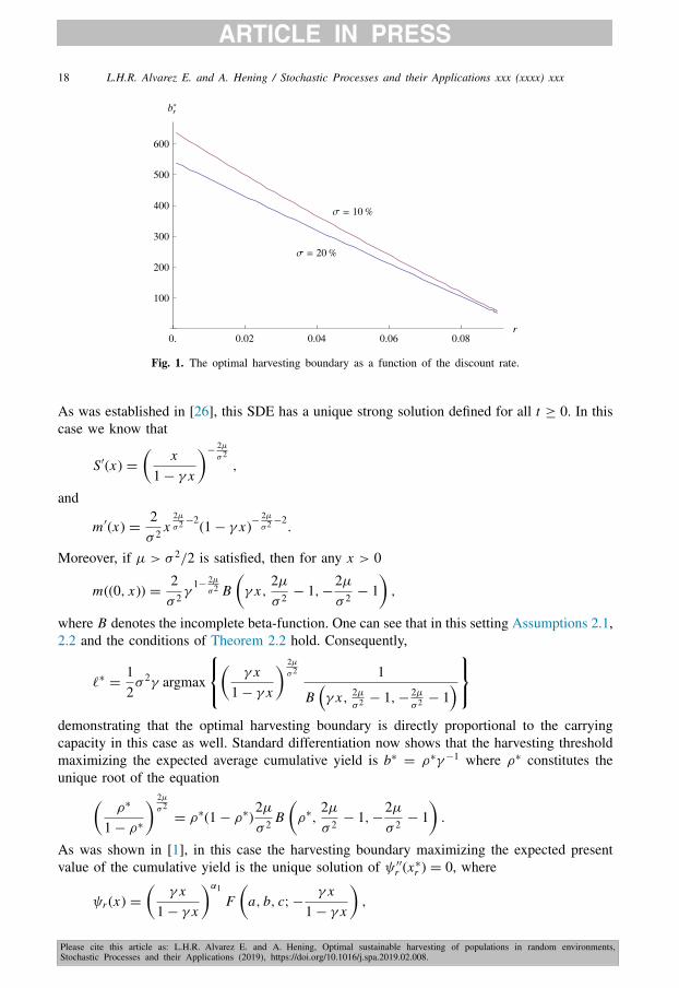
The optimal harvesting threshold is illustrated for two different volatilities as a function ofthe discount rate in Fig. 1 under the assumptions that µ = 0.1, γ = 0.001.

4.2. Logistic diffusion

An alternative logistic population growth model was studied in [26] and in [1]. The dynamicsis characterized by the stochastic differential equation

d X t = µX t (1 − γ X t )dt + σ X t (1 − γ X t )dWt , X0 = x ∈ (0, 1/γ ). (28)



Fig. 1. The optimal harvesting boundary as a function of the discount rate.

As was established in [26], this SDE has a unique strong solution defined for all t ≥ 0. In thiscase we know that

S′(x) =

(x

1 − γ x

)−2µσ2,

and

m ′(x) =2σ 2 x

2µσ2 −2(1 − γ x)−

2µσ2 −2

.

Moreover, if µ > σ 2/2 is satisfied, then for any x > 0

m((0, x)) =2σ 2 γ

1−2µσ2 B

(γ x,

2µσ 2 − 1,−

2µσ 2 − 1

),

where B denotes the incomplete beta-function. One can see that in this setting Assumptions 2.1,2.2 and the conditions of Theorem 2.2 hold. Consequently,

ℓ∗=

12σ 2γ argmax

⎧⎨⎩(

γ x1 − γ x

) 2µσ2 1

B(γ x, 2µ

σ 2 − 1,− 2µσ 2 − 1

)⎫⎬⎭

demonstrating that the optimal harvesting boundary is directly proportional to the carryingcapacity in this case as well. Standard differentiation now shows that the harvesting thresholdmaximizing the expected average cumulative yield is b∗

= ρ∗γ−1 where ρ∗ constitutes theunique root of the equation(

ρ∗

1 − ρ∗

) 2µσ2

= ρ∗(1 − ρ∗)2µσ 2 B

(ρ∗,

2µσ 2 − 1,−

2µσ 2 − 1

).

As was shown in [1], in this case the harvesting boundary maximizing the expected presentvalue of the cumulative yield is the unique solution of ψ ′′

r (x∗r ) = 0, where

ψr (x) =

(γ x

1 − γ x

)α1

F(

a, b, c; −γ x

1 − γ x

),



Fig. 2. The optimal harvesting boundary as a function of the discount rate.

F is the standard hypergeometric function,

a := 1 −α2

2+α1

2−

12

√(α2

2 − 2α2(2 + α1)) + (2 − α1)2,

b := 1 −α2

2+α1

2+

12

√(α2

2 − 2α2(2 + α1)) + (2 − α1)2,

and

c := 1 − α2 + α1.

We notice again that, as in the ergodic setting, the optimal threshold is directly proportional tothe carrying capacity.

The optimal harvesting threshold is illustrated for two different volatilities as a function ofthe discount rate in Fig. 2 under the assumptions that µ = 0.1, γ = 0.001.

5. Discussion

We investigated the optimal ergodic harvesting strategies of a population X whose dy-namics is given by a general one-dimensional stochastic differential equation. The theorywe develop for optimal sustainable harvesting includes the risks of extinction from envi-ronmental fluctuations (environmental stochasticity) as well as from harvesting. However, incontrast to most of the literature, we do not work with discount factors (see, for example,[1,5,24–26]) or maximal harvesting rates (see [17]). Instead, we concentrate on policies aimingto the maximization of the average cumulative yield. We proved that the optimal policy is ofthe same local time push type as in the discounted setting. Since the optimal threshold atwhich harvesting becomes optimal is a decreasing function of the prevailing discount rate, ourresults unambiguously demonstrate that policies based on ergodic (sustainable) criteria are moreprudent and imply higher population densities than models subject to discounting. Our resultsshow higher stochastic fluctuations negatively impact the population densities — this providesrigorous mathematical support for the arguments developed in [24] based on approximationarguments.



There are at least three directions in which our analysis could be extended. As was originallyestablished in [22] in a model based on controlled Brownian motion, the value of the optimalergodic policy is associated with the value of the finite horizon control problem

J (T, x) = supZ∈Λ

Ex [ZT ] ,

where T > 0 is a known fixed finite time horizon. It would be of interest whether an analogouslimiting result connects J (T, x)/T to l∗ in the general setting.

More recently, [33] considered the determination of the harvesting strategy maximizing theexpected present value of the cumulative yield from the present up to the extinction time in acase where the harvested population is subject to random regime switching characterized by anunderlying continuous time Markov chain (see also [14] for an application in forestry). Giventhe time homogeneity of the developed model, it would naturally be of interest to consider thedetermination of the harvesting policy maximizing the expected long run average yield in thatsetting as well.

Finally, the present analysis focuses on the harvesting of a single unstructured population.It would relevant to increasing the dimensionality of the considered model and introduceinteractions into the dynamics governing the evolution of the population stock (see for examplethe population dynamics models from [15,16,31]). In light of the studies [4,27], this latterproblem seems to be very challenging and is left for future considerations.

Acknowledgments

The authors are grateful to three anonymous referees for their constructive and detailedcomments.

References

[1] L.H.R. Alvarez E., Singular stochastic control in the presence of a state-dependent yield structure, StochasticProcess. Appl. 86 (2) (2000) 323–343.

[2] L.H.R. Alvarez E., Singular stochastic control, linear diffusions, and optimal stopping: a class of solvableproblems, SIAM J. Control Optim. 39 (6) (2001) 1697–1710.

[3] L.H.R. Alvarez E., A class of solvable impulse control problems, Appl. Math. Optim. 49 (2004) 265–295.[4] L.H.R. Alvarez E., E. Lungu, B. Øksendal, Optimal multi-dimensional stochastic harvesting with

density-dependent prices, Afr. Mat. 27 (3–4) (2016) 427–442.[5] L.H.R. Alvarez E., L.A. Shepp, Optimal harvesting of stochastically fluctuating populations, J. Math. Biol.

37 (2) (1998) 155–177.[6] A. Arapostathis, V.S. Borkar, M.K. Ghosh, Ergodic Control of Diffusion Processes, Vol. 143, Cambridge

University Press, 2012.[7] A.N. Borodin, P. Salminen, Handbook of Brownian Motion-facts and Formulae, Birkhäuser, 2015.[8] C.W. Clark, Mathematical Bioeconomics, third ed., in: Pure and Applied Mathematics (Hoboken), John Wiley

& Sons, Inc., Hoboken, NJ, 2010, p. xvi+368, The mathematics of conservation.[9] J. Drèze, N. Stern, The theory of cost-benefit analysis, Handb. Public Econ. 2 (1987) 909–989.

[10] H.J. Engelbert, W. Schmidt, Strong markov continuous local martingales and solutions of one-dimensionalstochastic differential equations (part iii), Math. Nachr. 151 (1) (1991) 149–197.

[11] S.N. Evans, A. Hening, S.J. Schreiber, Protected polymorphisms and evolutionary stability of patch-selectionstrategies in stochastic environments, J. Math. Biol. 71 (2) (2015) 325–359.

[12] J.A. Gulland, The Effect of Exploitation on the Numbers of Marine Animals, Proc. Adv. Study, Inst. DynamicsNumbers Popu, 1971, pp. 450–468.

[13] J.M. Harrison, Brownian Motion and Stochastic Flow Systems, Wiley, New York, 1985.[14] K.L. Helmes, R.H. Stockbridge, Thinning and harvesting in stochastic forest models, J. Econom. Dynam.

Control 35 (1) (2011) 25–39.

http://refhub.elsevier.com/S0304-4149(18)30348-X/sb1




































[15] A. Hening, D. Nguyen, Coexistence and extinction for stochastic Kolmogorov systems, Ann. Appl. Probab.28 (3) (2018) 1893–1942.

[16] A. Hening, D. Nguyen, Stochastic Lotka-Volterra food chains, J. Math. Biol. 77 (1) (2018) 135–163.[17] A. Hening, D.H. Nguyen, S.C. Ungureanu, T.K. Wong, Asymptotic harvesting of populations in random

environments, J. Math. Biol. (2018) (in press).[18] N. Ikeda, S. Watanabe, A comparison theorem for solutions of stochastic differential equations and its

applications, Osaka J. Math. 14 (3) (1977) 619–633.[19] N. Ikeda, S. Watanabe, Stochastic Differential Equations and Diffusion Processes, North-Holland Publishing

Co., Amsterdam, 1989.[20] A. Jack, M. Zervos, A singular control problem with an expected and a pathwise ergodic performance criterion,

J. Appl. Math. Stoch. Anal. (2006) 1–19.[21] O. Kallenberg, Foundations of Modern Probability, Springer, 2002.[22] I. Karatzas, A class of singular stochastic control problems, Adv. Appl. Probab. 15 (2) (1983) 225–254.[23] S. Karlin, H.M. Taylor, A Second Course in Stochastic Processes, Academic Press, Inc. [Harcourt Brace

Jovanovich, Publishers], New York-London, 1981, p. xviii+542.[24] R. Lande, S. Engen, B.E. Sæther, Optimal harvesting, economic discounting and extinction risk in fluctuating

populations, Nature 372 (1994) 88–90.[25] R. Lande, S. Engen, B.E. Sæther, Optimal harvesting of fluctuating populations with a risk of extinction,

Amer. Nat. 145 (5) (1995) 728–745.[26] E.M. Lungu, B. Øksendal, Optimal harvesting from a population in a stochastic crowded environment, Math.

Biosci. 145 (1) (1997) 47–75.[27] E. Lungu, B. Øksendal, Optimal harvesting from interacting populations in a stochastic environment, Bernoulli

7 (3) (2001) 527–539.[28] X. Mao, Stochastic Differential Equations and their Applications, in: Horwood Publishing Series in

Mathematics & Applications, Horwood Publishing Limited, Chichester, 1997.[29] R.B. Primack, Essentials of conservation biology, Sinauer Associates, Sunderland, Mass, 2006.[30] P.E. Protter, Stochastic Integration and Differential Equations, second ed., in: Stochastic Modelling and Applied

Probability, vol. 21, Springer-Verlag, Berlin, 2005, Version 2.1, Corrected third printing.[31] S.J. Schreiber, M. Benaïm, K.A.S. Atchadé, Persistence in fluctuating environments, J. Math. Biol. 62 (5)

(2011) 655–683.[32] S. Shreve, J. Lehoczky, D. Gaver, Optimal consumption for general diffusion with absorbing and reflecting

barriers, SIAM J. Control Optim. 22 (1984) 55–75.[33] Q. Song, R.H. Stockbridge, C. Zhu, On optimal harvesting problems in random environments, SIAM J. Control

Optim. 49 (2) (2011) 859–889.[34] M. Turelli, Random environments and stochastic calculus, Theor. Popul. Biol. 12 (2) (1977) 140–178.[35] A.P.N. Weerasinghe, Stationary stochastic control for Itô processes, Adv. Appl. Probab. 34 (1) (2002) 128–140.[36] A. Weerasinghe, An abelian limit approach to a singular ergodic control problem, SIAM J. Control Optim.

46 (2) (2007) 714–737.[37] T. Yamada, On a comparison theorem for solutions of stochastic differential equations and its applications,

J. Math. Kyoto Univ. 13 (1973) 497–512.[38] J. Yan, A comparison theorem for semimartingales and its applications, in: Séminaire de Probabilités, XX,

in: Lecture Notes in Mathematics, vol. 1204, 1986, pp. 349–351.





























































Documents

Optimal sustainable harvesting of populations in random