Optimal Transport for Machine Learning · = diag(a)Kdiag(b) eachiterationO(nm) complexity(matrixvector multiplication) canbeimprovedtoO(nlogn) ongriddedspacewith convolutions[Solomonetal

Optimal Transport for Machine Learning

Aude Genevay

CEREMADE (Université Paris-Dauphine)DMA (Ecole Normale Supérieure)MOKAPLAN Team (INRIA Paris)

Imaging in Paris - February 2018

Optimaltransport

AudeGenevay

EntropyRegularizedOT

Applicationsin Imaging

Large Scale"OT" forMachineLearning

Applicationto GenerativeModels

Outline

1 Entropy Regularized OT

2 Applications in Imaging

3 Large Scale "OT" for Machine Learning

4 Application to Generative Models

Optimaltransport

AudeGenevay





Shortcomings of OT

Two main issues when using OT in practice :• Poor sample complexity : need a lot of samples from µ andν to get a good approximation of W (µ, ν)

• Heavy computational cost : solving discrete OT requiressolving an LP → network simplex solver O(n3log(n)) [Peleand Werman ’09]

Optimaltransport

AudeGenevay





Entropy!

• Basically : Adding an entropic regularization smoothes theconstraint

• Makes the problem easier :• yields an unconstrained dual problem• discrete case can be solved efficiently with iterative

algorithm (more on that later)

• For ML applications, regularized Wasserstein is better thanstandard one

• In high dimension, helps avoiding overfitting

Optimaltransport

AudeGenevay





Entropic Relaxation of OT [Cuturi’13]

Add entropic penalty to Kantorovitch formulation of OT

minγ∈Π(µ,ν)

∫X×Y

c(x , y)dγ(x , y) + εKL(γ|µ⊗ ν)

where

KL(γ|µ⊗ ν)def.=

∫X×Y

(log( dγdµdν

(x , y))− 1)dγ(x , y)

Optimaltransport

AudeGenevay





Dual Formulation

maxu∈C(X )v∈C(Y)

∫Xu(x)dµ(x) +

∫Yv(y)dν(y)

−ε∫X×Y

eu(x)+v(y)−c(x,y)

ε dµ(x)dν(y)

Constraint in standard OT u(x) + v(y) < c(x , y) replaced by asmooth penalty term.

Optimaltransport

AudeGenevay





Dual Formulation

Dual problem concave in u and v , first order condition for eachvariable yield :

∇u = 0⇔ u(x) = −ε log(

∫Ye

v(y)−c(x,y)ε dν(y))

∇v = 0⇔ v(y) = −ε log(

∫Xe

u(x)−c(x,y)ε dµ(x))

Optimaltransport

AudeGenevay





The Discrete Case

Dual problem :

maxu∈Rmv∈Rn

n∑i=1

uiµi +m∑j=1

v jν j − εn,m∑i ,j=1

eui+vj−c(xi ,yj )

ε µiν j

First order conditions for each variable:

∇u = 0⇔ ui = −ε log(m∑j=1

evj−c(xi ,yj )

ε ν j)

∇v = 0⇔ v j = −ε log(n∑

i=1

eui−c(xi ,yj )

ε µi )

⇒ Do alternate maximizations!

Optimaltransport

AudeGenevay





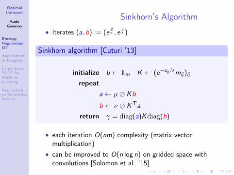
Sinkhorn’s Algorithm

• Iterates (a, b) := (euε , e

vε )

Sinkhorn algorithm [Cuturi ’13]

initialize b ← 1m K ← (e−cij/εmij)ij

repeata← µ� Kb

b ← ν � KTa

return γ = diag(a)Kdiag(b)

• each iteration O(nm) complexity (matrix vectormultiplication)

• can be improved to O(n log n) on gridded space withconvolutions [Solomon et al. ’15]

Optimaltransport

AudeGenevay





Sinkhorn - Toy Example

Marginals µ and ν

top : evolution of γ with number of iterations lbottom : evolution of γ with regularization parameter ε

Optimaltransport

AudeGenevay





Sinkhorn - Convergence

Definition (Hilbert metric)

Projective metric defined for x , y ∈ Rd++ by

dH(x , y) := logmaxi (xi/yi )mini (xi/yi )

TheoremThe iterates (a(l), b(l)) converge linearly for the Hilbert metric.

Remark : the contraction coefficient deteriorates quickly whenε→ 0 (exponentially in worst-case)

Optimaltransport

AudeGenevay





Sinkhorn - Convergence

Constraint violationWe have the following bound on the iterates:

dH(a(l), a?) ≤ κdH(γ1m, µ)

So monitoring the violation of the marginal constraints is a goodway to monitor convergence of Sinkhorn’s algorithm

‖γ1m − µ‖ for various regularizations

Optimaltransport

AudeGenevay





Color Transfer

Image courtesy of G. Peyré

Optimaltransport

AudeGenevay





Shape / Image BarycentersRegularized Wasserstein Barycenters [Nenna et al. ’15]

µ = argminµ∈Σn

Wε(µk , µ)

Image from [Solomon et al. ’15]

Optimaltransport

AudeGenevay





Sinkhorn loss

Consider entropy-regularized OT

minπ∈Π(µ,ν)

∫X×Y

c(x , y)dπ(x , y) + εKL(π|µ⊗ ν)

Regularized loss :

Wc,ε(µ, ν)def.=

∫XY

c(x , y)dπε(x , y)

where πε solution of (15)

Optimaltransport

AudeGenevay





Sinkhorn Divergences :interpolation between OT and

MMD

TheoremThe Sinkhorn loss between two measures µ, ν is defined as:

Wc,ε(µ, ν) = 2Wc,ε(µ, ν)−Wc,ε(µ, µ)−Wc,ε(ν, ν)

with the following limiting behavior in ε:1 as ε→ 0, Wc,ε(µ, ν)→ 2Wc(µ, ν)

2 as ε→ +∞, Wc,ε(µ, ν)→ ‖µ− ν‖−cwhere ‖·‖−c is the MMD distance whose kernel is minus the costfrom OT.

Remark : Some conditions are required on c to get MMDdistance when ε→∞. In particular, c = ‖·‖pp , 0 < p < 2 isvalid.

Optimaltransport

AudeGenevay





Sample Complexity

Sample Complexity of OT and MMD

Let µ a probability distribution on Rd , and µn an empiricalmeasure from µ

W (µ, µn) = O(n−1/d)

MMD(µ, µn) = O(n−1/2)

⇒ the number n of samples you need to get a precision η on theWassertein distance grows exponentially with the dimension d ofthe space!

Optimaltransport

AudeGenevay





Sample Complexity - Sinkhorn loss

Sample Complexity of Sinkhorn loss seems to improve as ε grows.

Plots courtesy of G. Peyré and M. Cuturi

Optimaltransport

AudeGenevay





Generative Models

Figure: Illustration of Density Fitting on a Generative Model

Optimaltransport

AudeGenevay





Density Fitting with Sinkhorn loss"Formally"

Solve minθ E (θ)

where E (θ)def.= Wc,ε(µθ, ν)

⇒ Issue : untractable gradient

Optimaltransport

AudeGenevay





Approximating Sinkhorn loss

• Rather than approximating the gradient approximate theloss itself

• Minibatches : E (θ)• sample x1, . . . , xm from µθ• use empirical Wasserstein distance Wc,ε(µθ, ν) whereµθ = 1

N

∑mi=1 δxi

• Use L iterations of Sinkhorn’s algorithm : E (L)(θ)• compute L steps of the algorithm• use this as a proxy for W (µθ, ν)

Optimaltransport

AudeGenevay





Computing the Gradient in Practice

C K

` ` + 1

SinkhornGenerative model ` = 1, . . . , L� 1

. . .

✓1✓2

(c(xi, yj))i,j

. . .

Input

data

(z1,.

..,z

m)

(x1,.

..,x

m)

(y1,.

..,y

n) 1m EL(✓)1/·

⇥mK>⇥nK

1/·

b`a`+1

b`+1

. . .. . .

h(C �K)bL, aLie�C/"

Figure: Scheme of the loss approximation

• Compute exact gradient of E (L)(θ) with autodiff• Backpropagation through above graph• Same computational cost as evaluation of E (L)(θ)

Optimaltransport

AudeGenevay





Numerical Results on MNIST (L2cost)

Figure: Samples from MNIST dataset

Optimaltransport

AudeGenevay






Figure: Fully connected NN with 2 hidden layers

Optimaltransport

AudeGenevay






Figure: Manifolds in the latent space for various parameters

Optimaltransport

AudeGenevay





Learning the cost [Li et al. ’17,Bellemare et al. ’17]

• On complex data sets, choice of a good ground metric c isnot trivial

• Use parametric cost function cφ(x , y) = ‖fφ(x)− fφ(y)‖22(where fφ : X → Rd )

• Optimization problem becomes minmax (like GANs)

minθmaxφWcφ,ε(µθ, ν)

• Same approximations but alternate between updating thecost parameters φ and the measure parameters θ

Optimaltransport

AudeGenevay





Numerical Results on CIFAR(learning the cost)

Figure: Samples from CIFAR dataset

Optimaltransport

AudeGenevay






Figure: Fully connected NN with 2 hidden layers

Optimaltransport

AudeGenevay






(a) MMD (b) ε = 1000 (c) ε = 10

Figure: Samples from the generator trained on CIFAR 10 for MMDand Sinkhorn loss (coming from the same samples in the latent space)

Which is better? Not just about generating nice images, butmore about capturing a high dimensional distribution... Hard toevaluate.

Optimaltransport

AudeGenevay





Shape Registration [Feydy et al.’17]

Documents

Optimal Transport for Machine Learning · = diag(a)Kdiag(b) eachiterationO(nm) complexity(matrixvector multiplication) canbeimprovedtoO(nlogn) ongriddedspacewith convolutions[Solomonetal