Embed Size (px)
Citation preview
Optimal Uncertainty Quantification
California Institute of Technology
AMSTAT Seminar
Mathematics Institute, University of Warwick, U.K.
18 March 2011
Sullivan & al. (Caltech) Optimal UQ Warwick, 18 March 2011 1 / 73

Collaborators and Support
Optimal UQ Theory:Mike McKerns, Michael Ortiz, Houman Owhadi (Caltech)Clint Scovel (Los Alamos National Laboratory)
Optimal UQ with Legacy Data:Dominik Meyer (Technische Universitat Munchen)Florian Theil (University of Warwick)
Multiphase Steel ApplicationDaniel Balzani (Universitat Duisberg-Essen)
Portions of this work were supported by the United States Department of Energy
National Nuclear Security Administration under Award Number DE-FC52-08NA28613
through the California Institute of Technology’s ASC/PSAAP Center for the Predictive
Modeling and Simulation of High Energy Density Dynamic Response of Materials.
Sullivan & al. (Caltech) Optimal UQ Warwick, 18 March 2011 2 / 73
Outline
1 Introduction
2 Optimal Uncertainty Quantification
3 Consequences of Optimal UQ
4 Computational Examples
5 Further Work and Conclusions
Sullivan & al. (Caltech) Optimal UQ Warwick, 18 March 2011 3 / 73

Introduction
Introduction
Sullivan & al. (Caltech) Optimal UQ Warwick, 18 March 2011 4 / 73

Introduction Uncertainty Quantification
What is Uncertainty Quantification?
?
Sullivan & al. (Caltech) Optimal UQ Warwick, 18 March 2011 5 / 73
Introduction Uncertainty Quantification
What is Uncertainty Quantification?
Sullivan & al. (Caltech) Optimal UQ Warwick, 18 March 2011 5 / 73
Introduction Uncertainty Quantification
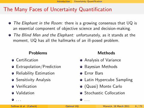
The Many Faces of Uncertainty Quantification
The Elephant in the Room: there is a growing consensus that UQ isan essential component of objective science and decision-making.
The Blind Men and the Elephant: unfortunately, as it stands at themoment, UQ has all the hallmarks of an ill-posed problem.
Problems
Certification
Extrapolation/Prediction
Reliability Estimation
Sensitivity Analysis
Verification
Validation
. . .
Methods
Analysis of Variance
Bayesian Methods
Error Bars
Latin Hypercube Sampling
(Quasi) Monte Carlo
Stochastic Collocation
. . .
Sullivan & al. (Caltech) Optimal UQ Warwick, 18 March 2011 6 / 73
Introduction Uncertainty Quantification
Types of Uncertainty
Uncertainties are often divided into two types: epistemic and aleatoricuncertainties.〈1〉
An epistemic uncertainty is one that stems from a fundamental lackof knowledge — we don’t know the rules that govern the problem.
An aleatoric uncertainty is one that stems from intrinsic randomnessin the system — a “roll of the dice”.
The conventional wisdom is that aleatoric uncertainties are “nicer”than epistemic uncertainties, because the powerful tools of probabilitytheory can be brought to bear.
〈1〉W. L. Oberkampf, T. G. Trucano & C. Hirsch (2004) “Verification, validation, andpredictive capability in computational engineering and physics” ASME Appl. Mech. Rev.
57(5):345–384.Sullivan & al. (Caltech) Optimal UQ Warwick, 18 March 2011 7 / 73
Introduction Uncertainty Quantification
Types of Uncertainty
However, on close inspection, many apparently aleatoric uncertaintiesare epistemic: are you really sure that important parameter X isuniformly distributed, or has sub-Gaussian tails?
Therefore, theoreticians and practitioners alike tend to be somewhatskeptical of probabilistic methods — “probabilistic reliability studiesinvolve assumptions on the probability densities, whose knowledgeregarding relevant input quantities is central.”〈2〉
On the other hand, UQ methods based on deterministic worst-casescenarios are oftentimes “too pessimistic to be practical.”〈3〉
〈2〉I. Elishakoff & M. Ohsaki (2010) Optimization and Anti-Optimization of Structures
Under Uncertainty. World Scientific, London.〈3〉R. F. Drenick (1973) “Aseismic design by way of critical excitation” J. Eng. Mech.
Div., Am. Soc. Civ. Eng. 99:649–667.Sullivan & al. (Caltech) Optimal UQ Warwick, 18 March 2011 8 / 73
Introduction Uncertainty Quantification
Optimal Uncertainty Quantification
We propose a mathematical framework for UQ as an optimizationproblem, which we call Optimal Uncertainty Quantification (OUQ), inwhich knowledge (ǫπιστηµη) lies at the heart of the problemformulation.
The development and application of OUQ to real, complex problemsis a collaborative interdisciplinary effort that requires expertise (andstimulates developments) in
pure and applied mathematics, especially probability theory,numerical optimization,(massively) parallel computing,the application area (e.g. biology, chemistry, economics, engineering,geoscience, meteorology, physics, . . . ).
Sullivan & al. (Caltech) Optimal UQ Warwick, 18 March 2011 9 / 73
Introduction Uncertainty Quantification
Optimal Uncertainty Quantification
In a nutshell, the OUQ viewpoint is the following:
OUQ is the business of computing optimal bounds on quantities
of interest that are themselves functions of unknown functions
and unknown probability measures, where “optimality” means
that those bounds are the sharpest ones possible given the
available information on those unknowns.
This paradigm is easiest to explain in the prototypical context of thecertification problem (bounding probabilities of failure). There will besome remarks about other contexts at the end of the talk.
Sullivan & al. (Caltech) Optimal UQ Warwick, 18 March 2011 10 / 73
Introduction Certification
The Certification Problem
Suppose that you are interested in a system of interest, G : X → R,which is a real-valued function of some random inputs X ∈ X withprobability distribution P on X .
Some value θ ∈ R is a performance threshold: if G(X) ≤ θ, then thesystem fails; if G(X) > θ, then the system succeeds.
You want to know the probability of failure
P[G(X) ≤ θ],
or at least to know if it exceeds some prescribed maximum acceptableprobability of failure ǫ — but you do not know G and P!
If you have some information about G and P, what are the bestrigorous lower and upper bounds that you can give on the probabilityof failure using that information?
Sullivan & al. (Caltech) Optimal UQ Warwick, 18 March 2011 11 / 73
Introduction Certification
The Certification Problem
The challenge, then, is to bound P[G(X) ≤ θ] given someinformation on or assumptions about G and P.
Optimality of the bounds is important — the following bounds aretrue, but useless:
0 ≤ P[G(X) ≤ θ] ≤ 1.
Robustness of the bounds is also important — i.e. to know that thebounds and any safe/unsafe decisions are stable with respect toperturbations of the information/assumptions.
Sullivan & al. (Caltech) Optimal UQ Warwick, 18 March 2011 12 / 73

Introduction Certification
The Importance of Optimalityand Robustness. Being overlyconservative may lead to hugeeconomic losses, but being overlyoptimistic may lead to loss of life,environmental damage & c.
Eyjafjallajokull, Iceland, 27 March 2010
Space Shuttle Columbia, 1 February 2003
Deepwater Horizon, 21 April 2010
Sullivan & al. (Caltech) Optimal UQ Warwick, 18 March 2011 13 / 73

Introduction Certification
Standard UQ Methods
So, how can one show that P[G(X) ≤ θ] ≤ ǫ when G and P are onlyimperfectly known?
Monte Carlo methods?We need many independent P-distributed samples of G(X): naıveMC needs O(ǫ−2 log ǫ−1) samples; QMC needs O(ǫ−1(log ǫ−1)dimX )samples and G to be “well-behaved”.
Stochastic collocation methods?We need a good representation for P and rapid decay of thespectrum, and easy exercise of G.
Bayesian inference?We need prior distributions in which we genuinely believe; also, if thepriors and “reality” disagree greatly, then it may take a very largedata set to “correct” the priors into posteriors that are close to“reality”, which is vital if the important events are prior-rare.
Sullivan & al. (Caltech) Optimal UQ Warwick, 18 March 2011 14 / 73
Introduction Certification
Standard UQ Methods
Each of these methods relies, implicitly or explicitly, on the validity ofcertain assumptions in order to be applicable — or at least efficient.This leads to three main difficulties:
the assumptions may not match the information about G and P;the assumptions may vary from method to method, which makes faircomparisons of different methods difficult;the assumptions often cannot be easily perturbed.
Therefore, in formulating OUQ, we choose to place information onand assumptions about G and P at the centre of the problem.
This goes one step beyond Babuska’s commandment “thou shaltconfess thy sins”: in OUQ, your sins precisely describe your problem!
Sullivan & al. (Caltech) Optimal UQ Warwick, 18 March 2011 15 / 73
Optimal Uncertainty Quantification
Optimal UncertaintyQuantification
Sullivan & al. (Caltech) Optimal UQ Warwick, 18 March 2011 16 / 73
Optimal Uncertainty Quantification Formulating the Problem
What Problem Should You Solve?
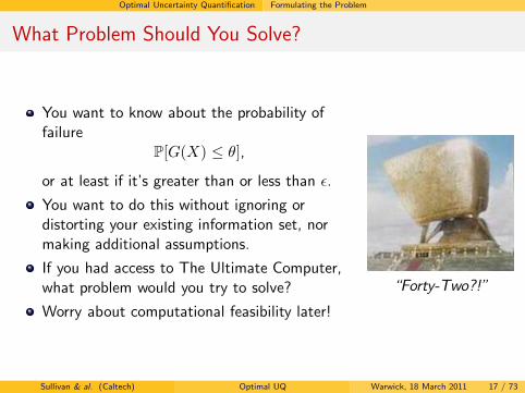
You want to know about the probability offailure
P[G(X) ≤ θ],
or at least if it’s greater than or less than ǫ.
You want to do this without ignoring ordistorting your existing information set, normaking additional assumptions.
If you had access to The Ultimate Computer,what problem would you try to solve?
Worry about computational feasibility later!
“Forty-Two?!”
Sullivan & al. (Caltech) Optimal UQ Warwick, 18 March 2011 17 / 73
Optimal Uncertainty Quantification Formulating the Problem
Information / Assumptions
Write down all the information that you have about the system. Forexample, this information might come from
physical laws;expert opinion;experimental data.
Let A denote the set of all pairs (f, µ) that are consistent with yourinformation about (G,P):
A ⊆
{(f, µ)
∣∣∣∣f : X → R is measurable, andµ is a probability measure on X
}.
All you know about reality is that (G,P) ∈ A; any (f, µ) ∈ A is anadmissible scenario for the unknown reality (G,P).
A is a huge space (probably infinite-dimensional and non-separable inany example of interest); the need to explore it efficiently motivatesthe reduction theorems that will come later.
Sullivan & al. (Caltech) Optimal UQ Warwick, 18 March 2011 18 / 73
Optimal Uncertainty Quantification Formulating the Problem
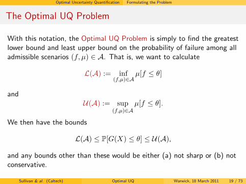
The Optimal UQ Problem
With this notation, the Optimal UQ Problem is simply to find the greatestlower bound and least upper bound on the probability of failure among alladmissible scenarios (f, µ) ∈ A. That is, we want to calculate
L(A) := inf(f,µ)∈A
µ[f ≤ θ]
andU(A) := sup
(f,µ)∈Aµ[f ≤ θ].
We then have the bounds
L(A) ≤ P[G(X) ≤ θ] ≤ U(A),
and any bounds other than these would be either (a) not sharp or (b) notconservative.
Sullivan & al. (Caltech) Optimal UQ Warwick, 18 March 2011 19 / 73
Optimal Uncertainty Quantification Formulating the Problem
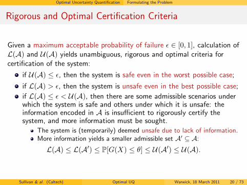
Rigorous and Optimal Certification Criteria
Given a maximum acceptable probability of failure ǫ ∈ [0, 1], calculation ofL(A) and U(A) yields unambiguous, rigorous and optimal criteria forcertification of the system:
if U(A) ≤ ǫ, then the system is safe even in the worst possible case;
if L(A) > ǫ, then the system is unsafe even in the best possible case;
if L(A) ≤ ǫ < U(A), then there are some admissible scenarios underwhich the system is safe and others under which it is unsafe: theinformation encoded in A is insufficient to rigorously certify thesystem, and more information must be sought.
The system is (temporarily) deemed unsafe due to lack of information.More information yields a smaller admissible set A′ ⊆ A:
L(A) ≤ L(A′) ≤ P[G(X) ≤ θ] ≤ U(A′) ≤ U(A).
Sullivan & al. (Caltech) Optimal UQ Warwick, 18 March 2011 20 / 73
Optimal Uncertainty Quantification Examples of OUQ Information Sets
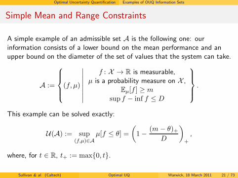
Simple Mean and Range Constraints
A simple example of an admissible set A is the following one: ourinformation consists of a lower bound on the mean performance and anupper bound on the diameter of the set of values that the system can take.
A :=
(f, µ)
∣∣∣∣∣∣∣∣
f : X → R is measurable,µ is a probability measure on X ,
Eµ[f ] ≥ msup f − inf f ≤ D
.
This example can be solved exactly:
U(A) := sup(f,µ)∈A
µ[f ≤ θ] =
(1−
(m− θ)+D
)
+
,
where, for t ∈ R, t+ := max{0, t}.
Sullivan & al. (Caltech) Optimal UQ Warwick, 18 March 2011 21 / 73

Optimal Uncertainty Quantification Examples of OUQ Information Sets
More Complicated Mean and Range Constraints
On a product space X := X1 × · · · × XK , consider
AMcD :=
(f, µ)
∣∣∣∣∣∣∣∣∣∣
f : X → R,
Dk[f ] := sup |f(x1, . . . , xk, . . . , xK)−
− f(x1, . . . , xk, . . . , xK)| ≤ Dk,µ = µ1 ⊗ · · · ⊗ µK on X ,
Eµ[f ] ≥ m
.
These are the assumptions of McDiarmid’s inequality〈4〉 (a.k.a. thebounded differences inequality), which gives the upper bound
U(AMcD) ≤ exp
(−2(m− θ)2+∑K
k=1D2k
).
〈4〉C. McDiarmid (1989) “On the method of bounded differences” Surveys in
Combinatorics, 1989, Camb. Univ. Press, 148–188.Sullivan & al. (Caltech) Optimal UQ Warwick, 18 March 2011 22 / 73
Optimal Uncertainty Quantification Examples of OUQ Information Sets
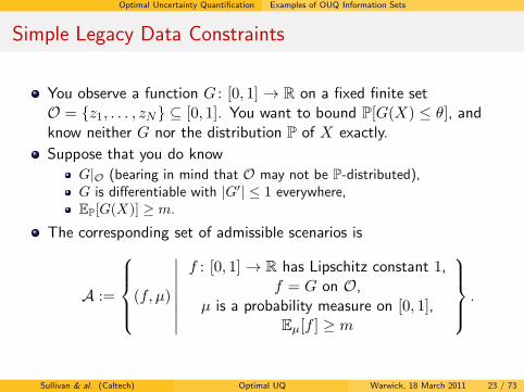
Simple Legacy Data Constraints
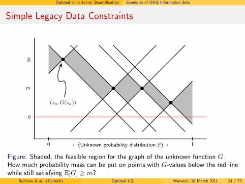
You observe a function G : [0, 1]→ R on a fixed finite setO = {z1, . . . , zN} ⊆ [0, 1]. You want to bound P[G(X) ≤ θ], andknow neither G nor the distribution P of X exactly.
Suppose that you do know
G|O (bearing in mind that O may not be P-distributed),G is differentiable with |G′| ≤ 1 everywhere,EP[G(X)] ≥ m.
The corresponding set of admissible scenarios is
A :=
(f, µ)
∣∣∣∣∣∣∣∣
f : [0, 1]→ R has Lipschitz constant 1,f = G on O,
µ is a probability measure on [0, 1],Eµ[f ] ≥ m
.
Sullivan & al. (Caltech) Optimal UQ Warwick, 18 March 2011 23 / 73
Optimal Uncertainty Quantification Examples of OUQ Information Sets
Simple Legacy Data Constraints
b
(zn, G(zn))
b b
b
R
m
θ
0 1←(Unknown probability distribution P)→
Figure: Shaded, the feasible region for the graph of the unknown function G.How much probability mass can be put on points with G-values below the red linewhile still satisfying E[G] ≥ m?
Sullivan & al. (Caltech) Optimal UQ Warwick, 18 March 2011 24 / 73

Optimal Uncertainty Quantification Examples of OUQ Information Sets
More Complicated Legacy Data Constraints
More generally, the unknown function G may be a function of manyindependent inputs of unknown distribution. Whatever information wehave about the smoothness of G becomes a constraint on the smoothnessof the admissible scenarios f :
A :=
(f, µ)
∣∣∣∣∣∣∣∣∣∣
f : X → R is measurable,µ = µ1 ⊗ · · · ⊗ µK on X ,
f = G on O,〈some smoothness conditions on f〉,
Eµ[f ] ≥ m
.
Sullivan & al. (Caltech) Optimal UQ Warwick, 18 March 2011 25 / 73

Optimal Uncertainty Quantification Finite-Dimensional Reduction
Reduction of OUQ
OUQ problems are global, infinite-dimensional, non-convex,highly-constrained (i.e. nasty!) optimization problems.
The non-convexity is a fact of life, but there are powerful reductiontheorems that allow a reduction to a search space of low dimension.
Instead of searching over all admissible probability measures µ, weneed only to search over those with a very simple “extremal”structure: in the simplest case, these are just finite sums of pointmasses (Dirac measures) on the input parameter space X .
That is, we can “pretend” that all the random inputs are discreterandom variables and just optimize over the possible values andprobabilities that those discrete variables might take.
Sullivan & al. (Caltech) Optimal UQ Warwick, 18 March 2011 26 / 73
Optimal Uncertainty Quantification Finite-Dimensional Reduction
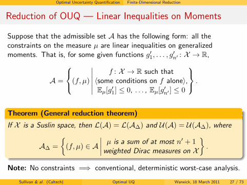
Reduction of OUQ — Linear Inequalities on Moments
Suppose that the admissible set A has the following form: all theconstraints on the measure µ are linear inequalities on generalizedmoments. That is, for some given functions g′1, . . . , g
′n′ : X → R,
A =
(f, µ)
∣∣∣∣∣∣
f : X → R such that〈some conditions on f alone〉,Eµ[g
′1] ≤ 0, . . . , Eµ[g
′n′ ] ≤ 0
.
Theorem (General reduction theorem)
If X is a Suslin space, then L(A) = L(A∆) and U(A) = U(A∆), where
A∆ =
{(f, µ) ∈ A
∣∣∣∣µ is a sum of at most n′ + 1weighted Dirac measures on X
}.
Note: No constraints =⇒ conventional, deterministic worst-case analysis.
Sullivan & al. (Caltech) Optimal UQ Warwick, 18 March 2011 27 / 73
Optimal Uncertainty Quantification Finite-Dimensional Reduction
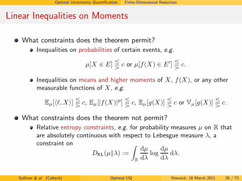
Linear Inequalities on Moments
What constraints does the theorem permit?
Inequalities on probabilities of certain events, e.g.
µ[X ∈ E] S c or µ[f(X) ∈ E′] S c.
Inequalities on means and higher moments of X , f(X), or any othermeasurable functions of X , e.g.
Eµ[〈ℓ,X〉] S c, Eµ[|f(X)|p] S c, Eµ[g(X)] S c or Vµ[g(X)] S c.
What constraints does the theorem not permit?
Relative entropy constraints, e.g. for probability measures µ on R thatare absolutely continuous with respect to Lebesgue measure λ, aconstraint on
DKL(µ‖λ) :=
∫
R
dµ
dλlog
dµ
dλdλ.
Sullivan & al. (Caltech) Optimal UQ Warwick, 18 March 2011 28 / 73
Optimal Uncertainty Quantification Finite-Dimensional Reduction
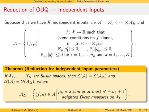
Reduction of OUQ — Independent Inputs
Suppose that we have K independent inputs, i.e. X = X1 × · · · × XK and
A =
(f, µ)
∣∣∣∣∣∣∣∣∣∣
f : X → R such that〈some conditions on f alone〉,
µ = µ1 ⊗ · · · ⊗ µK ,Eµ[g
′1] ≤ 0, . . . , Eµ[g
′n′ ] ≤ 0,
Eµk[gki ] ≤ 0 for i = 1, . . . , nk and k = 1, . . . ,K
.
Theorem (Reduction for independent input parameters)
If X1, . . . , XK are Suslin spaces, then L(A) = L(A∆) andU(A) = U(A∆), where
A∆ =
{(f, µ) ∈ A
∣∣∣∣µk is a sum of at most n′ + nk + 1weighted Dirac measures on Xk
}.
Sullivan & al. (Caltech) Optimal UQ Warwick, 18 March 2011 29 / 73
Optimal Uncertainty Quantification Finite-Dimensional Reduction
Reduction of OUQ — Legacy Problem
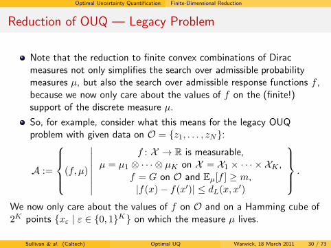
Note that the reduction to finite convex combinations of Diracmeasures not only simplifies the search over admissible probabilitymeasures µ, but also the search over admissible response functions f ,because we now only care about the values of f on the (finite!)support of the discrete measure µ.
So, for example, consider what this means for the legacy OUQproblem with given data on O = {z1, . . . , zN}:
A :=
(f, µ)
∣∣∣∣∣∣∣∣
f : X → R is measurable,µ = µ1 ⊗ · · · ⊗ µK on X = X1 × · · · × XK ,
f = G on O and Eµ[f ] ≥ m,|f(x)− f(x′)| ≤ dL(x, x
′)
.
We now only care about the values of f on O and on a Hamming cube of2K points {xε | ε ∈ {0, 1}
K} on which the measure µ lives.
Sullivan & al. (Caltech) Optimal UQ Warwick, 18 March 2011 30 / 73
Optimal Uncertainty Quantification Finite-Dimensional Reduction
Reduction of OUQ — Legacy Problem
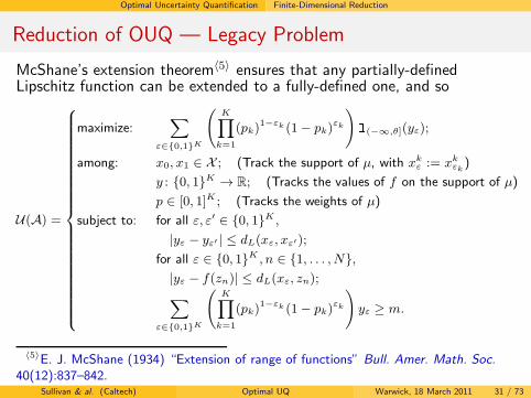
McShane’s extension theorem〈5〉 ensures that any partially-definedLipschitz function can be extended to a fully-defined one, and so
U(A) =
maximize:∑
ε∈{0,1}K
(
K∏
k=1
(pk)1−εk (1− pk)
εk
)1(−∞,θ](yε);
among: x0, x1 ∈ X ; (Track the support of µ, with xkε := xk
εk)
y : {0, 1}K → R; (Tracks the values of f on the support of µ)
p ∈ [0, 1]K ; (Tracks the weights of µ)
subject to: for all ε, ε′ ∈ {0, 1}K ,
|yε − yε′ | ≤ dL(xε, xε′);
for all ε ∈ {0, 1}K , n ∈ {1, . . . , N},
|yε − f(zn)| ≤ dL(xε, zn);
∑
ε∈{0,1}K
(
K∏
k=1
(pk)1−εk (1− pk)
εk
)
yε ≥ m.
〈5〉E. J. McShane (1934) “Extension of range of functions” Bull. Amer. Math. Soc.
40(12):837–842.Sullivan & al. (Caltech) Optimal UQ Warwick, 18 March 2011 31 / 73

Consequences of Optimal UQ
Consequences of Optimal UQ
Sullivan & al. (Caltech) Optimal UQ Warwick, 18 March 2011 32 / 73
Consequences of Optimal UQ Optimal Concentration Inequalities
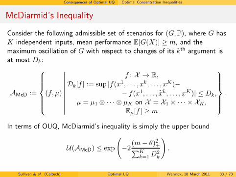
McDiarmid’s Inequality
Consider the following admissible set of scenarios for (G,P), where G hasK independent inputs, mean performance E[G(X)] ≥ m, and themaximum oscillation of G with respect to changes of its kth argument isat most Dk:
AMcD :=
(f, µ)
∣∣∣∣∣∣∣∣∣∣
f : X → R,
Dk[f ] := sup |f(x1, . . . , xk, . . . , xK)−
− f(x1, . . . , xk, . . . , xK)| ≤ Dk,µ = µ1 ⊗ · · · ⊗ µK on X = X1 × · · · × XK ,
Eµ[f ] ≥ m
.
In terms of OUQ, McDiarmid’s inequality is simply the upper bound
U(AMcD) ≤ exp
(−2
(m− θ)2+∑Kk=1D
2k
).
Sullivan & al. (Caltech) Optimal UQ Warwick, 18 March 2011 33 / 73
Consequences of Optimal UQ Optimal Concentration Inequalities
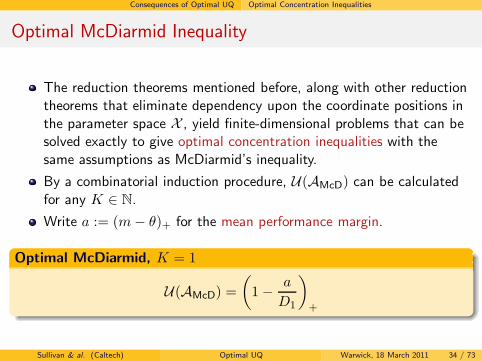
Optimal McDiarmid Inequality
The reduction theorems mentioned before, along with other reductiontheorems that eliminate dependency upon the coordinate positions inthe parameter space X , yield finite-dimensional problems that can besolved exactly to give optimal concentration inequalities with thesame assumptions as McDiarmid’s inequality.
By a combinatorial induction procedure, U(AMcD) can be calculatedfor any K ∈ N.
Write a := (m− θ)+ for the mean performance margin.
Optimal McDiarmid, K = 1
U(AMcD) =
(1−
a
D1
)
+
Sullivan & al. (Caltech) Optimal UQ Warwick, 18 March 2011 34 / 73
Consequences of Optimal UQ Optimal Concentration Inequalities
Optimal McDiarmid Inequality
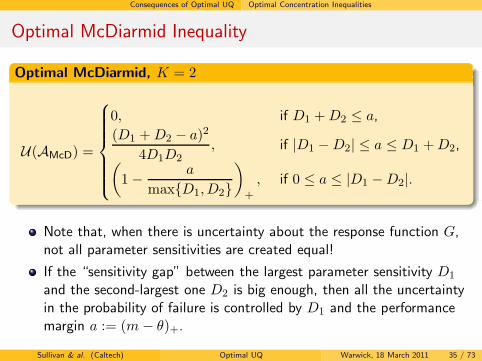
Optimal McDiarmid, K = 2
U(AMcD) =
0, if D1 +D2 ≤ a,
(D1 +D2 − a)2
4D1D2, if |D1 −D2| ≤ a ≤ D1 +D2,
(1−
a
max{D1,D2}
)
+
, if 0 ≤ a ≤ |D1 −D2|.
Note that, when there is uncertainty about the response function G,not all parameter sensitivities are created equal!
If the “sensitivity gap” between the largest parameter sensitivity D1
and the second-largest one D2 is big enough, then all the uncertaintyin the probability of failure is controlled by D1 and the performancemargin a := (m− θ)+.
Sullivan & al. (Caltech) Optimal UQ Warwick, 18 March 2011 35 / 73
Consequences of Optimal UQ Optimal Concentration Inequalities
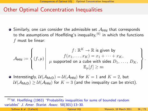
Other Optimal Concentration Inequalities
Similarly, one can consider the admissible set AHfd that correspondsto the assumptions of Hoeffding’s inequality,〈6〉 in which the functionsf must be linear:
AHfd :=
(f, µ)
∣∣∣∣∣∣∣∣
f : RK → R is given byf(x1, . . . , xK) = x1 + · · ·+ xK ,
µ supported on a cube with sides D1, . . . , DK ,Eµ[f ] ≥ m
.
Interestingly, U(AMcD) = U(AHfd) for K = 1 and K = 2, butU(AMcD) ≥ U(AHfd) for K = 3 (and the inequality can be strict).
〈6〉W. Hoeffding (1963) “Probability inequalities for sums of bounded randomvariables” J. Amer. Statist. Assoc. 58(301):13–30.
Sullivan & al. (Caltech) Optimal UQ Warwick, 18 March 2011 36 / 73
Consequences of Optimal UQ The OUQ Loop
The OUQ Loop
The calculation of extremal probabilities of failure over a fixedadmissible set A is not the end of the game.
A strength of the OUQ viewpoint is that the assumptions/constraintsthat determine A can be perturbed to see if the conclusions arerobust with respect to those changes.
Inconclusive results and sensitive assumptions can be selected forfurther experimentation — and the OUQ process itself can be used toidentify the most informative experiments.
Sullivan & al. (Caltech) Optimal UQ Warwick, 18 March 2011 37 / 73
Consequences of Optimal UQ The OUQ Loop
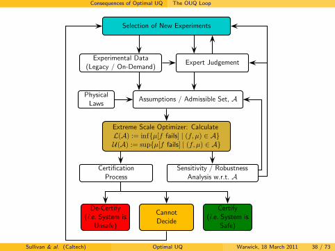
Selection of New Experiments
Experimental Data(Legacy / On-Demand)
Expert Judgement
PhysicalLaws
Assumptions / Admissible Set, A
Extreme Scale Optimizer: CalculateL(A) := inf{µ[f fails] | (f, µ) ∈ A}U(A) := sup{µ[f fails] | (f, µ) ∈ A}
CertificationProcess
Sensitivity / RobustnessAnalysis w.r.t. A
De-Certify(i.e. System is
Unsafe)
CannotDecide
Certify(i.e. System is
Safe)
Sullivan & al. (Caltech) Optimal UQ Warwick, 18 March 2011 38 / 73
Consequences of Optimal UQ Experimental Selection
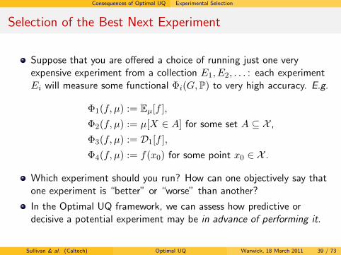
Selection of the Best Next Experiment
Suppose that you are offered a choice of running just one veryexpensive experiment from a collection E1, E2, . . . : each experimentEi will measure some functional Φi(G,P) to very high accuracy. E.g.
Φ1(f, µ) := Eµ[f ],
Φ2(f, µ) := µ[X ∈ A] for some set A ⊆ X ,
Φ3(f, µ) := D1[f ],
Φ4(f, µ) := f(x0) for some point x0 ∈ X .
Which experiment should you run? How can one objectively say thatone experiment is “better” or “worse” than another?
In the Optimal UQ framework, we can assess how predictive ordecisive a potential experiment may be in advance of performing it.
Sullivan & al. (Caltech) Optimal UQ Warwick, 18 March 2011 39 / 73
Consequences of Optimal UQ Experimental Selection
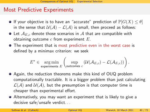
Most Predictive Experiments
If your objective is to have an “accurate” prediction of P[G(X) ≤ θ]in the sense that U(A)− L(A) is small, then proceed as follows:
Let AE,c denote those scenarios in A that are compatible withobtaining outcome c from experiment E.
The experiment that is most predictive even in the worst case isdefined by a minimax criterion: we seek
E∗ ∈ argminexperiments E
(sup
outcomes c(U(AE,c)−L(AE,c))
).
Again, the reduction theorems make this kind of OUQ problemcomputationally tractable. It is a bigger problem than just calculatingL(A) and U(A), but the presumption is that computer time ischeaper than experimental effort.
Alternatively, you may want an experiment that is likely to give adecisive safe/unsafe verdict. . .
Sullivan & al. (Caltech) Optimal UQ Warwick, 18 March 2011 40 / 73
Consequences of Optimal UQ Experimental Selection
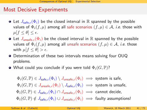
Most Decisive Experiments
Let Jsafe,ǫ(Φi) be the closed interval in R spanned by the possiblevalues of Φi(f, µ) among all safe scenarios (f, µ) ∈ A, i.e. those withµ[f ≤ θ] ≤ ǫ.
Let Junsafe,ǫ(Φi) be the closed interval in R spanned by the possiblevalues of Φi(f, µ) among all unsafe scenarios (f, µ) ∈ A, i.e. thosewith µ[f ≤ θ] > ǫ.
Determination of these two intervals means solving four OUQproblems.
What could you conclude if you were told Φi(G,P)?
Φi(G,P) ∈ Jsafe,ǫ(Φi) \ Junsafe,ǫ(Φi) =⇒ system is safe,
Φi(G,P) ∈ Junsafe,ǫ(Φi) \ Jsafe,ǫ(Φi) =⇒ system is unsafe,
Φi(G,P) ∈ Jsafe,ǫ(Φi) ∩ Junsafe,ǫ(Φi) =⇒ cannot decide,
Φi(G,P) /∈ Jsafe,ǫ(Φi) ∪ Junsafe,ǫ(Φi) =⇒ faulty assumptions!
Sullivan & al. (Caltech) Optimal UQ Warwick, 18 March 2011 41 / 73
Consequences of Optimal UQ Experimental Selection
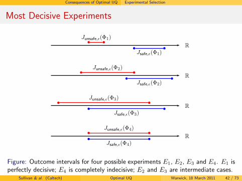
Most Decisive Experiments
R
Junsafe,ǫ(Φ1)
Jsafe,ǫ(Φ1)
R
Junsafe,ǫ(Φ2)
Jsafe,ǫ(Φ2)
R
Junsafe,ǫ(Φ3)
Jsafe,ǫ(Φ3)
R
Junsafe,ǫ(Φ4)
Jsafe,ǫ(Φ4)
Figure: Outcome intervals for four possible experiments E1, E2, E3 and E4. E1 isperfectly decisive; E4 is completely indecisive; E2 and E3 are intermediate cases.
Sullivan & al. (Caltech) Optimal UQ Warwick, 18 March 2011 42 / 73
Consequences of Optimal UQ Experimental Selection
Selection of Experimental Campaigns
This idea of experimental selection can be extended to plan severalexperiments in advance, i.e. to plan campaigns of experiments.
This is a kind of infinite-dimensional Cluedo, played on spaces ofadmissible scenarios, against our lack of perfect information aboutreality, and made tractable by the reduction theorems.
Sullivan & al. (Caltech) Optimal UQ Warwick, 18 March 2011 43 / 73

Consequences of Optimal UQ Relevant and Redundant Observations
Relevant and Redundant Legacy Data
In many UQ applications, it is important to know which legacy data arethose that have any — or the most — relevance to the UQ problem athand. In this framework, the relevance of legacy data enters naturally interms of the constraints: relevant data points correspond to non-trivialconstraints.
Definition
Given a set of observations of G on O ⊆ X , say that an observation of Gat z∗ ∈ X is redundant on S ⊆ X with respect to O if, whenever theconstraints from G|O are satisfied on S, so is the constraint from G(z∗),i.e.
for all n ∈ {1, . . . , N},for all x ∈ S and y ∈ R,|y −G(zn)| ≤ dL(x, zn)
=⇒ |y −G(z∗)| ≤ dL(x, z∗).
Sullivan & al. (Caltech) Optimal UQ Warwick, 18 March 2011 44 / 73
Consequences of Optimal UQ Relevant and Redundant Observations
Relevant and Redundant Legacy Data
R
S X \ S
bb
b
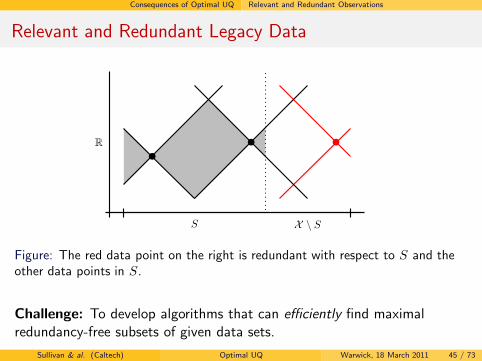
Figure: The red data point on the right is redundant with respect to S and theother data points in S.
Challenge: To develop algorithms that can efficiently find maximalredundancy-free subsets of given data sets.
Sullivan & al. (Caltech) Optimal UQ Warwick, 18 March 2011 45 / 73
Computational Examples
Computational Examples
Sullivan & al. (Caltech) Optimal UQ Warwick, 18 March 2011 46 / 73
Computational Examples Example 1: Hypervelocity Impact
Example 1: Hypervelocity Impact
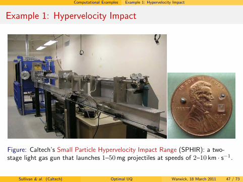
Figure: Caltech’s Small Particle Hypervelocity Impact Range (SPHIR): a two-stage light gas gun that launches 1–50mg projectiles at speeds of 2–10 km · s−1.
Sullivan & al. (Caltech) Optimal UQ Warwick, 18 March 2011 47 / 73
Computational Examples Example 1: Hypervelocity Impact
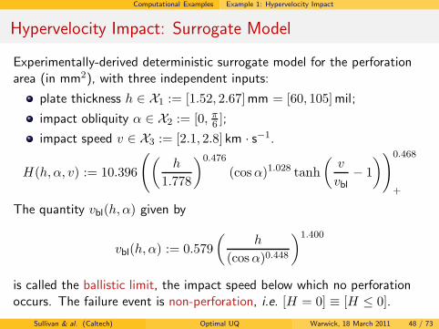
Hypervelocity Impact: Surrogate Model
Experimentally-derived deterministic surrogate model for the perforationarea (in mm2), with three independent inputs:
plate thickness h ∈ X1 := [1.52, 2.67]mm = [60, 105]mil;
impact obliquity α ∈ X2 := [0, π6 ];
impact speed v ∈ X3 := [2.1, 2.8] km · s−1.
H(h, α, v) := 10.396
((h
1.778
)0.476
(cosα)1.028 tanh
(v
vbl− 1
))0.468
+
The quantity vbl(h, α) given by
vbl(h, α) := 0.579
(h
(cosα)0.448
)1.400
is called the ballistic limit, the impact speed below which no perforationoccurs. The failure event is non-perforation, i.e. [H = 0] ≡ [H ≤ 0].
Sullivan & al. (Caltech) Optimal UQ Warwick, 18 March 2011 48 / 73
Computational Examples Example 1: Hypervelocity Impact
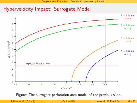
Hypervelocity Impact: Surrogate Model
1.4 1.6 1.8 2.0 2.2 2.4 2.6 2.80
1
2
3
4
5
6
7
8
9
v/km · s−1
H(h,α,v)/mm
2
impactor footprint area
h = 1.52mmα = 0
h = 1.52mmα = π
6
h = 2.67mmα = 0
h = 2.67mmα = π
6
Figure: The surrogate perforation area model of the previous slide.
Sullivan & al. (Caltech) Optimal UQ Warwick, 18 March 2011 49 / 73
Computational Examples Example 1: Hypervelocity Impact
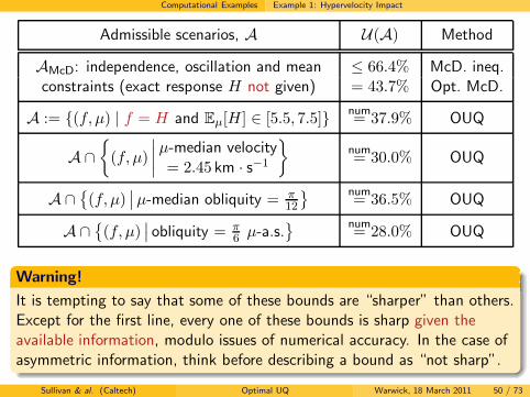
Admissible scenarios, A U(A) Method
AMcD: independence, oscillation and mean ≤ 66.4% McD. ineq.constraints (exact response H not given) = 43.7% Opt. McD.
A := {(f, µ) | f = H and Eµ[H] ∈ [5.5, 7.5]}num= 37.9% OUQ
A ∩
{(f, µ)
∣∣∣∣µ-median velocity
= 2.45 km · s−1
}num= 30.0% OUQ
A ∩{(f, µ)
∣∣µ-median obliquity = π12
} num= 36.5% OUQ
A ∩{(f, µ)
∣∣ obliquity = π6 µ-a.s.
} num= 28.0% OUQ
Warning!
It is tempting to say that some of these bounds are “sharper” than others.Except for the first line, every one of these bounds is sharp given theavailable information, modulo issues of numerical accuracy. In the case ofasymmetric information, think before describing a bound as “not sharp”.
Sullivan & al. (Caltech) Optimal UQ Warwick, 18 March 2011 50 / 73
Computational Examples Example 1: Hypervelocity Impact
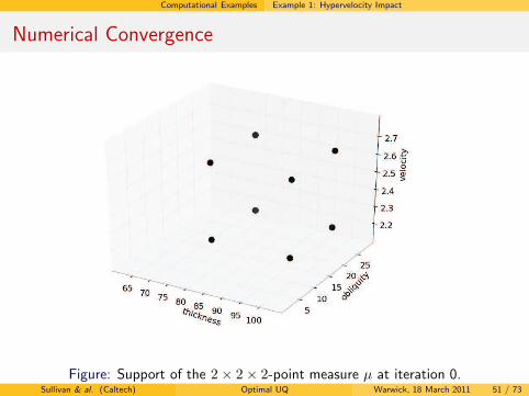
Numerical Convergence
Figure: Support of the 2× 2× 2-point measure µ at iteration 0.Sullivan & al. (Caltech) Optimal UQ Warwick, 18 March 2011 51 / 73
Computational Examples Example 1: Hypervelocity Impact
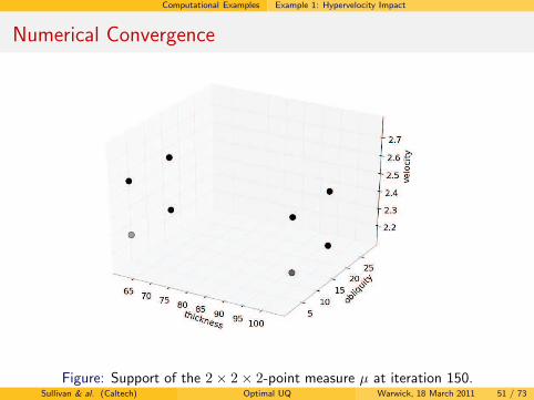
Numerical Convergence
Figure: Support of the 2× 2× 2-point measure µ at iteration 150.Sullivan & al. (Caltech) Optimal UQ Warwick, 18 March 2011 51 / 73
Computational Examples Example 1: Hypervelocity Impact
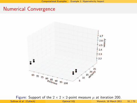
Numerical Convergence
Figure: Support of the 2× 2× 2-point measure µ at iteration 200.Sullivan & al. (Caltech) Optimal UQ Warwick, 18 March 2011 51 / 73

Computational Examples Example 1: Hypervelocity Impact
Numerical Convergence
Figure: Support of the 2× 2× 2-point measure µ at iteration 1000.Sullivan & al. (Caltech) Optimal UQ Warwick, 18 March 2011 51 / 73
Computational Examples Example 1: Hypervelocity Impact
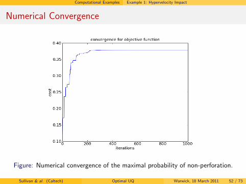
Numerical Convergence
Figure: Numerical convergence of the maximal probability of non-perforation.
Sullivan & al. (Caltech) Optimal UQ Warwick, 18 March 2011 52 / 73
Computational Examples Example 1: Hypervelocity Impact
Numerical Convergence
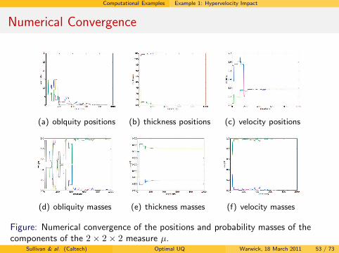
(a) oblquity positions (b) thickness positions (c) velocity positions
(d) obliquity masses (e) thickness masses (f) velocity masses
Figure: Numerical convergence of the positions and probability masses of thecomponents of the 2× 2× 2 measure µ.
Sullivan & al. (Caltech) Optimal UQ Warwick, 18 March 2011 53 / 73
Computational Examples Example 1: Hypervelocity Impact
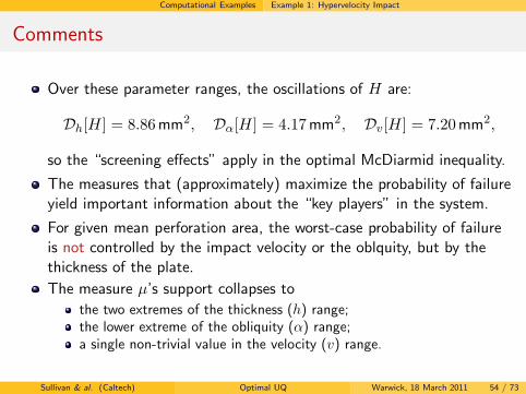
Comments
Over these parameter ranges, the oscillations of H are:
Dh[H] = 8.86mm2, Dα[H] = 4.17mm2, Dv[H] = 7.20mm2,
so the “screening effects” apply in the optimal McDiarmid inequality.
The measures that (approximately) maximize the probability of failureyield important information about the “key players” in the system.
For given mean perforation area, the worst-case probability of failureis not controlled by the impact velocity or the oblquity, but by thethickness of the plate.
The measure µ’s support collapses to
the two extremes of the thickness (h) range;the lower extreme of the obliquity (α) range;a single non-trivial value in the velocity (v) range.
Sullivan & al. (Caltech) Optimal UQ Warwick, 18 March 2011 54 / 73
Computational Examples Example 2: Seismic Safety Certification
Example 2: Seismic Safety Certification
Now consider a more involved example: the safety of a truss structureunder an earthquake.
For simplicity, we consider a purely elastic response in a trussstructure composed of
N joints, with positions u(t) ∈ R3N ;
J members, with axial strains y(t) ∈ RJ ;
member j has yield strength Sj , so the structure is safe if
minj=1,...,J
(Sj − ‖yj‖∞) > 0,
and fails otherwise.
Sullivan & al. (Caltech) Optimal UQ Warwick, 18 March 2011 55 / 73
Computational Examples Example 2: Seismic Safety Certification
Equations of Motion
The time evolution of the structure is governed by the second-orderODE
Mu+ Cu+Ku = f ,
where M , C and K are the symmetric positive-definite 3N × 3Nmass, damping and stiffness matrices, and f collects anyexternally-applied loads (e.g. wind loads).
We work instead with v := u− Tγ, i.e. u less the motion obtained byrigid translation according to the ground motion:
Mv + Cv +Kv = f −MTγ.
Let L ∈ RJ×3N map v to the array of member strains, so that
yj = (Lv)j .
Sullivan & al. (Caltech) Optimal UQ Warwick, 18 March 2011 56 / 73

Computational Examples Example 2: Seismic Safety Certification
Response Function
Given a history of ground motion acceleration γ, it is astraightforward calculation in a nodal basis for the structure and usinghereditary integrals to solve for v and hence to check the safety of thestructure according to the safety criterion
minj=1,...,J
(Sj − ‖yj‖∞) > 0.
This relationship is deterministic. Randomness enters the problem viathe ground motion acceleration, which we treat as a timeconvolution:〈7〉
γ0 = ψ ⋆ s,
where s is the earthquake source and ψ the transfer function.
〈7〉S. Stein & M. Wysession (2002) An Introduction to Seismology, Earthquakes, and
Earth Structure. Wiley–Blackwell.Sullivan & al. (Caltech) Optimal UQ Warwick, 18 March 2011 57 / 73
Computational Examples Example 2: Seismic Safety Certification
Ground Motion Acceleration
A reasonable representation for s is as a sequence of I boxcar timeimpulses of random but independent duration and amplitude:
s =
I∑
i=1
Xi1[∑i−1k=1 τk,
∑ik=1 τk]
with independent random Xi in [−amax, amax]3 of mean 0 and τk in
[0, τmax] having mean E[τk] ∈ [τ1, τ2].
Similarly, we express the (unknown) transfer function with respect tosome basis of a discretization of the time interval of interest — say, ofdimension Q.
Reasonable values for all these parameters (amax, I, & c.) can befound in the literature.〈8〉
〈8〉L. Esteva (1970) “Seismic risk and seismic design” in Seismic Design for Nuclear
Power Plants The MIT Press.Sullivan & al. (Caltech) Optimal UQ Warwick, 18 March 2011 58 / 73
Computational Examples Example 2: Seismic Safety Certification
Application of OUQ Reduction Theorems
Crucially, the OUQ reduction theorems apply to give a reduced OUQproblem of dimension 18I +Q since
there are no constraints on the transfer function (and so the optimizerwill find the deterministically “worst” one — one Dirac mass), andthere are Q such deterministic components;the mean constraints on the three components of each Xi generate aneed for four Dirac masses, and there are I of these;the mean constraints on each τk generate need for two Dirac masses,and there are I of these.
Sullivan & al. (Caltech) Optimal UQ Warwick, 18 March 2011 59 / 73
Computational Examples Example 2: Seismic Safety Certification
Critical Excitation
Without constraints, worst-case scenarios correspond to focusing theenergy of the earthquake in modes of resonances of the structure.
Without correlations in the ground motion these scenarios correspondto rare events in which independent random variables must conspireto strongly excite a specific resonance mode.
The lack of information on the transfer function ψ and the meanvalues E[τk] permits scenarios characterized by strong correlations inground motion where the energy of the earthquake can be focused inthe above-mentioned modes of resonance.
Sullivan & al. (Caltech) Optimal UQ Warwick, 18 March 2011 60 / 73

Computational Examples Example 3: Multiphase Steels
Example 3: Multiphase Steels
Advanced High-Strength Steels (AHSS)offer many advantages in e.g. automobileconstruction:
light-weight construction;
enhanced crash safety.
AHSS have complex microstructure,involving two or more phases, leading toa complex macroscopic response(anisotropy, kinematic hardening, & c.).Significant sources of uncertaintyinclude:
microstructure morphology;
material properties of individualphases.
From www.bmw.de
Sullivan & al. (Caltech) Optimal UQ Warwick, 18 March 2011 61 / 73
Computational Examples Example 3: Multiphase Steels
Description of the Material Problem
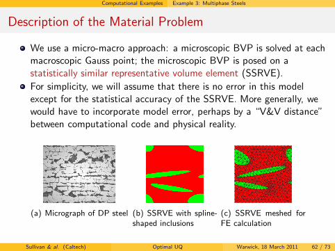
We use a micro-macro approach: a microscopic BVP is solved at eachmacroscopic Gauss point; the microscopic BVP is posed on astatistically similar representative volume element (SSRVE).
For simplicity, we will assume that there is no error in this modelexcept for the statistical accuracy of the SSRVE. More generally, wewould have to incorporate model error, perhaps by a “V&V distance”between computational code and physical reality.
(a) Micrograph of DP steel (b) SSRVE with spline-shaped inclusions
(c) SSRVE meshed forFE calculation
Sullivan & al. (Caltech) Optimal UQ Warwick, 18 March 2011 62 / 73
Computational Examples Example 3: Multiphase Steels
Description of the Material Problem
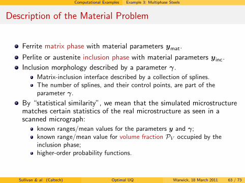
Ferrite matrix phase with material parameters ymat.
Perlite or austenite inclusion phase with material parameters yinc.
Inclusion morphology described by a parameter γ.
Matrix-inclusion interface described by a collection of splines.The number of splines, and their control points, are part of theparameter γ.
By “statistical similarity”, we mean that the simulated microstructurematches certain statistics of the real microstructure as seen in ascanned micrograph:
known ranges/mean values for the parameters y and γ;known range/mean value for volume fraction PV occupied by theinclusion phase;higher-order probability functions.
Sullivan & al. (Caltech) Optimal UQ Warwick, 18 March 2011 63 / 73
Computational Examples Example 3: Multiphase Steels
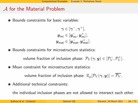
A for the Material Problem
Bounds constraints for basic variables:
γ ∈ [γ−,γ+],
yinc ∈ [y−inc,y
+inc],
ymat ∈ [y−mat,y
+mat].
Bounds constraints for microstructure statistics:
volume fraction of inclusion phase: PV (γ,y) ∈ [P−V ,P
+V ].
Mean constraint for microstructure statistics:
volume fraction of inclusion phase: Eµ[PV (γ,y)] = PV .
Additional technical constraints:
the individual inclusion phases are not allowed to intersect each other.
Sullivan & al. (Caltech) Optimal UQ Warwick, 18 March 2011 64 / 73
Computational Examples Example 3: Multiphase Steels
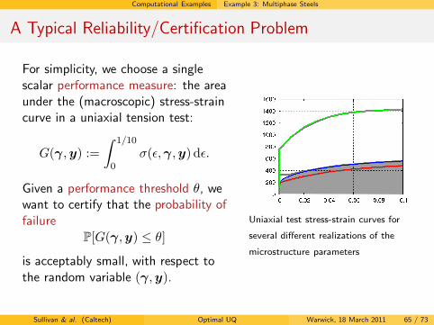
A Typical Reliability/Certification Problem
For simplicity, we choose a singlescalar performance measure: the areaunder the (macroscopic) stress-straincurve in a uniaxial tension test:
G(γ,y) :=
∫ 1/10
0σ(ǫ,γ,y) dǫ.
Given a performance threshold θ, wewant to certify that the probability offailure
P[G(γ,y) ≤ θ]
is acceptably small, with respect tothe random variable (γ,y).
Uniaxial test stress-strain curves for
several different realizations of the
microstructure parameters
Sullivan & al. (Caltech) Optimal UQ Warwick, 18 March 2011 65 / 73

Further Work and Conclusions
Further Work and Conclusions
Sullivan & al. (Caltech) Optimal UQ Warwick, 18 March 2011 66 / 73
Further Work and Conclusions Further Work: Other UQ Problems
Other UQ Problems
Certification — as in the bounding of probabilities of failure — is notthe only UQ problem.
However, certification appears to be a central and prototypical UQproblem; many other UQ problems can be posed as certificationproblems.
For example, verification and validation problems are very easilytransformed into certification problems.
“Verification deals with mathematics; validation deals withphysics”,〈9〉 but otherwise the two problems are very similar.
〈9〉P. J. Roache (1998) Verification and Validation in Computational Science and
Engineering. Hermosa Publ., Albuquerque.Sullivan & al. (Caltech) Optimal UQ Warwick, 18 March 2011 67 / 73
Further Work and Conclusions Further Work: Other UQ Problems
Verification
Verification of a computational model means showing that it is“acceptably close” to the mathematical description of the processesthat it is supposed to model.
Let U denote the exact mathematical solution to the problem, and Fthe computational model.
The verification problem is now to show that
P[‖U(X) − F (X)‖ ≤ θ] ≥ 1− ǫ
for suitable threshold values θ and ǫ, a suitable norm/distance ‖ · ‖,and with P-distributed input parameters X taking values in someverification domain.
Sullivan & al. (Caltech) Optimal UQ Warwick, 18 March 2011 68 / 73
Further Work and Conclusions Further Work: Other UQ Problems
Validation
Validation of a computational model means showing that it is“acceptably close” to the processes that it is supposed to model. (Inverification, the problem is mathematical; in validation, the problem isphysical.)
Let F denote the computational model and P the physical process.
The validation problem is now to show that
P[‖F (X) − P (X)‖ ≤ θ] ≥ 1− ǫ
for suitable threshold values θ and ǫ, a suitable norm/distance ‖ · ‖,and with P-distributed input parameters X taking values in somevalidation domain.
Sullivan & al. (Caltech) Optimal UQ Warwick, 18 March 2011 69 / 73
Further Work and Conclusions Further Work: Other UQ Problems
Prediction
What is a “prediction” about some real-valued quantity of interestG(X)? In a loose sense, it is an interval [a, b] ⊆ R (hopefully “assmall as possible”) such that
P[a ≤ G(X) ≤ b] ≈ 1.
In the OUQ paradigm, this can be made more precise: given acollection of admissible scenarios A for (G,P), and ǫ > 0, we seek
sup
{a ∈ R
∣∣∣∣ inf(f,µ)∈A
µ[f ≥ a] ≥ 1−ǫ
2
},
inf
{b ∈ R
∣∣∣∣ inf(f,µ)∈A
µ[f ≤ b] ≥ 1−ǫ
2
}.
Sullivan & al. (Caltech) Optimal UQ Warwick, 18 March 2011 70 / 73
Further Work and Conclusions Further Work: OUQ with Sample Data
Optimal UQ with Random Sample Data
Another area of research is what it means to give optimal bounds onthe probability of failure when the information is not justdeterministic, but also comes from random sample data.
If we are told that we will observe a realization D of sample datafrom a space D (e.g. ten IID samples), we seek an “upper-bounder”Ψ: D → [0, 1] such that
inf(f,µ)∈A
µD[Ψ(D) ≥ µ[f ≤ θ]
]≥ 1− ǫ,
and we want Ψ to be “minimal” in some sense.
This is a very delicate issue, with great scope for supplier–clientconflict and the classical paradoxes of voting theory (e.g. Arrow’stheorem) to intrude.
However, it does appear that there is a connection between OUQwith sample data and the notion of a Uniformly Most Powerfulhypothesis test.
Sullivan & al. (Caltech) Optimal UQ Warwick, 18 March 2011 71 / 73
Further Work and Conclusions Conclusions
Conclusions
UQ is an essential component of modern science, with manyhigh-consequence applications. However, there is no establishedconsensus on how to formally pose “the UQ problem”, nor a commonlanguage in which to communicate and quantitatively compare UQmethods and results.
OUQ is an opening gambit. OUQ is not just an effort to provideanswers, but an effort to well-pose the question: OUQ is thechallenge of optimally bounding functions of unknown responses andunknown probabilities, given some information about them.
A key feature is that the OUQ viewpoint explicitly requires the user toexplicitly state all the assumptions in operation — once listed, theycan be perturbed to see if the answers are robust.
Although the optimization problems involved are large, in many casesof interest, their dimension can be substantially reduced.
Sullivan & al. (Caltech) Optimal UQ Warwick, 18 March 2011 72 / 73
Further Work and Conclusions References
References
H. Owhadi, C. Scovel, T. J. Sullivan, M. McKerns & M. Ortiz.“Optimal Uncertainty Quantification” (2010)Submitted to SIAM Review. Preprint at
http://arxiv.org/pdf/1009.0679v1
Optimization calculations performed using mystic:
http://dev.danse.us/trac/mystic
Sullivan & al. (Caltech) Optimal UQ Warwick, 18 March 2011 73 / 73