Optimisation of maintenance routing and scheduling for offshore wind farms

Chandra Ade Irawan1,* Djamila Ouelhadj1, Dylan Jones1, Magnus Stålhane2, Iver Bakken Sperstad3

1Centre for Operational Research and Logistics, Department of Mathematics, University of Portsmouth,

Lion Gate Building, Lion Terrace, Portsmouth, PO1 3HF, UK 2Department of Industrial Economics and Technology Management, Norwegian University of Science and

Technology, Alfred Getz veg 3, 7491 Trondheim, Norway 3SINTEF Energy Research, P.O. Box 4761 Sluppen, NO-7465 Trondheim, Norway

Abstract An optimisation model and a solution method for maintenance routing and

scheduling at offshore wind farms are proposed. The model finds the optimal schedule for

maintaining the turbines and the optimal routes for the crew transfer vessels to service the

turbines along with the number of technicians required for each vessel. The model takes into

account multiple vessels, multiple periods (days), multiple Operation & Maintenance (O&M)

bases, and multiple wind farms. We develop an algorithm based on the Dantzig-Wolfe

decomposition method, where a mixed integer linear program is solved for each subset of

turbines to generate all feasible routes and maintenance schedules for the vessels for each

period. The routes have to consider several constraints such as weather conditions, the

availability of vessels, and the number of technicians available at the O&M base. An integer

linear program model is then proposed to find the optimal route configuration along with the

maintenance schedules that minimise maintenance costs, including travel, technician and

penalty costs. The computational experiments show that the proposed optimisation model and

solution method find optimal solutions to the problem in reasonable computing times.

Key words: Maintenance scheduling, routing problem, offshore wind farm.

1. Introduction

The development of offshore wind farms has been significant over the past 20 years. One

of the reasons for this growth is that a wind turbine at sea generally produces more electricity

than that of its onshore equivalent as the average wind speed at sea is higher. However, the

installation, operation, and maintenance costs are also much higher for offshore wind

* Corresponding Author. Tel.: +44(0)23 9284 6367. Email address: chandra.irawan@port.ac.uk

1

brought to you by COREView metadata, citation and similar papers at core.ac.uk

provided by Portsmouth University Research Portal (Pure)

turbines, since more resources and infrastructures are needed to install and maintain a wind

turbine at sea. According to Snyder and Kaiser (2009), the operations and maintenance costs

could contribute a quarter of the life-cycle costs, making it one of the largest cost components

of an offshore wind farm. One way to reduce the costs is to make the maintenance activities

more efficient by optimising maintenance schedules and the routing of maintenance vessels.

This potential for cost reduction becomes increasingly important as wind farms become

larger and constructed farther from shore, increasing the vessel travel times both to and

within the wind farms.

According to European Committee for Standardization (2010), maintenance activities in

wind power systems involve corrective maintenance, predetermined (preventive)

maintenance, and condition-based maintenance. Corrective maintenance is performed

following detection of a failure where the aim of this maintenance is to restore normal

operating conditions. Predetermined preventive maintenance is conducted at predetermined

intervals or based on prescribed criteria such as the age of the equipment and production

schedule. This maintenance aims to reduce the failure risk or performance degradation of the

equipment. Condition-based maintenance is done by assessing the actual equipment condition

using inspection or (on-line) condition monitoring. The maintenance activity is performed

when there are indicators which give information that the system is deteriorating and the

probability of failure is rising. In this paper, we deal with the maintenance scheduling

problem where the recommended period for a set of turbines that need to be maintained is

given. The turbines can be selected based on the principles of predetermined preventive

maintenance or condition-based maintenance. A penalty cost is incurred in the model when

the maintenance activity is performed after the recommended period.

Maintenance scheduling for offshore wind farms is a complex and challenging problem

(Shafiee, 2015). The main goal of maintenance scheduling is to construct a detailed schedule

of maintenance activities that have to be performed within a planning horizon. There are

several factors that need to be considered when scheduling the maintenance activities of an

offshore wind farm including the weather conditions, the availability of various resources

(e.g. service vessels, crews, and spare parts), and the disruption to electricity generation.

Resources needed for maintaining the offshore turbines are commonly based at the nearest

port or Operation & Maintenance (O&M) base. The weather conditions (such as wind speed

and wave height) and the vessel availability are the main factors that affect the performance

of the maintenance activities. For safety reasons, the maintenance can only be performed in

2

periods where the required weather conditions are met. As good weather periods are limited

in most locations where wind farms are currently located or being planned, maintenance

schedules must be optimised to exploit the resulting weather windows. Once the maintenance

schedules have been fixed (the period when the turbines in the wind farms will be

serviced/visited), other aspects required to be addressed are as follows: the type of vessels

that will be used for each period; the optimal route for each selected vessel to visit the set of

turbines in the wind farms; and the number of each skill type of technicians required by each

vessel for the given maintenance schedule and vessel route. Therefore, the maintenance

problem of an offshore wind farm is a complex problem and difficult to solve to optimality.

The main contributions of this paper include: (i) Presenting a new routing and scheduling

problem from the offshore wind industry that considers several logistics bases and the

possibility of servicing more than one wind farms with the same fleet. (ii) Proposing a new

mathematical model and solution method to solve the problem. (iii) Obtaining new optimal

solutions for a set of benchmark problems from the literature along with the solutions for new

more challenging problems.

The paper is organised as follows: Section 2 presents a description of the maintenance

routing and scheduling problem for offshore wind farms, a brief review on maintenance

scheduling in offshore wind farms, and an overview of related routing problems. Section 3

gives a description of the maintenance routing and scheduling problem for offshore wind

farm. Section 4 presents the optimisation model and solution method for solving the

maintenance routing and scheduling problem. Section 5 presents the computational results on

the data available in the literature and new randomly generated data. The last section provides

a summary of our findings and some avenues for future research.

2. Literature Review

2.1 Maintenance routing and scheduling for offshore wind farms

The maintenance routing and scheduling problem for an offshore wind farm was

introduced by Dai et al. (2015). The problem consists of finding one route and schedule for

each vessel to perform maintenance on a set of wind turbines over a planning period of

several days. The model takes into account a penalty cost if the turbines are maintained after

the recommended period. The model also considers the capacity of vessels in transporting

3

technicians and spare parts. Stålhane et al. (2015) study the problem proposed by Dai et al.

(2015), but consider only one period. They propose an arc-flow model of the problem, and

reformulate it as a path-flow model by using Dantzig-Wolfe decomposition (Dantzig and

Wolfe (1960)). The re-formulated problem is solved as a mixed integer program, where a

subset of possible routes and schedules are generated heuristically.

The papers mentioned above only consider one O&M base and one wind farm. However,

some wind farm operators or O&M service providers may serve multiple offshore wind farms

in the same area, and may use multiple ports as the base for conducting O&M. This may be

increasingly relevant to consider as more clusters of neighbouring wind farms are being

developed, allowing more resources to being shared between them. To the best of our

knowledge, there is no paper in the literature dealing with maintenance routing and

scheduling problem for multiple wind farms and O&M bases. Therefore, in this paper, we

propose a new mathematical model and a solution method to tackle such a problem. In

addition, we take into account the number of each skill type of technicians available at each

O&M base, the availability of the vessels and spare parts, and the ability of a vessel to

transfer spare parts.

2.2 Review on maintenance scheduling problems for offshore wind farms

This subsection presents an overview of related maintenance scheduling problems from

the wind energy sector. We begin by giving an overview of predetermined preventive

maintenance scheduling, and then presenting papers studying corrective and condition-based

maintenance scheduling.

Predetermined preventive maintenance

A mathematical model for determining the best time for maintenance operations taking

into account the performance of the wind turbine and the availability of the resources was

built by Kovács et al. (2011). Parikh (2012) proposed a mathematical model to optimise the

maintenance cost of wind farms by scheduling preventive maintenance and replacement of

critical components. An optimal preventive maintenance scheduling model for minimising

the overall downtime energy losses was studied by Zhang et al. (2012). The model takes into

account weather conditions, crews, transportation, and tooling infrastructure. A model for the

preventive maintenance scheduling of power plants including wind farms was proposed by

Perez-Canton and Rubio-Romero (2013), which aims to maximise the system reliability.

4

Corrective and condition-based maintenance

There are several papers that study scheduling of corrective and condition based

maintenance operations. An opportunistic maintenance optimization model taking into

account wind forecasts and corrective maintenance activities was studied by Besnard et al.

(2009). Besnard et al. (2011) extended their previous work by formulating a stochastic

optimisation problem that considers uncertainty in weather conditions. Byon et al. (2011)

used the discrete event system specification (DEVS) to build a simulation model for wind

farm operations and maintenance where two different maintenance strategies, namely

scheduled maintenance and condition-based maintenance are applied. The results showed that

condition-based maintenance yields more wind power generation by reducing wind turbine

failure rates. Van Horenbeek et al. (2012) investigated prognostic maintenance scheduling for

offshore wind turbines where the added value of a prognostic maintenance policy was

quantified. Camci (2015) studied a methodology to schedule the maintenance of

geographically distributed assets using their prognostic information which can be applied for

maintenance scheduling at offshore wind farm.

The previous works cited on optimal scheduling of maintenance in this subsection have

not considered how to access the turbines that need to be maintained. This is taken into

account in the routing and scheduling problem presented in this paper.

2.3 Related routing problems

The routing and scheduling problem of maintenance vessels at offshore wind farms can

be categorized as a vehicle routing problem with pick-up and delivery (VRPDP) according to

the classification scheme provided in the survey conducted by Berbeglia et al. (2007). As the

survey shows, the most successful exact solution approach for this type of pickup and

delivery problems is based on a Dantzig-Wolfe decomposition of the original mathematical

formulation (Dantzig and Wolfe, 1960). When applying the Dantzig-Wolfe decomposition

method to a vehicle routing problem (VRP), one obtains a master problem that consists of

selecting one route for each vehicle, such that all customers are serviced exactly once. The

corresponding sub-problems determine the set of feasible routes and their corresponding

costs. For problems where the number of feasible routes is relatively small, all routes can be

generated a priori, and the master problem can then be solved as an integer program.

Otherwise new routes can be generated dynamically in each node of the Branch-and-Bound

5

tree, a method known as branch-and-price (Barnhart et al. 1998). This approach has been

used successfully to solve different versions of the one-to-one VRPDP by, among others,

Dumas et al. (1991), Savelsbergh and Sol (1998), Røpke and Cordeau (2009), Brønmo et al.

(2010) and Baldacci et al. (2011).

The routing and scheduling problem of maintenance vessels at offshore wind farms also

incorporates elements from an extension of the one-to-one VRPDP known as the Dial-a-Ride

Problem (DARP). According to Cordeau and Laporte (2007), DARP problems often include

quality of service criteria such as maximum route duration and customer ride times. At

offshore wind farms the length of a shift and the width of the weather window for a given

vessel limits the maximum route duration, while the requirement of a minimum elapsed time

between when the technicians are delivered to a turbine and picked up again are the opposite

of customer ride time considerations where a maximum time between pickup and delivery is

enforced. Thus, similar to the DARP, it is insufficient to find the optimal route for each

vessel that performs maintenance at the offshore wind farm; one must also find the optimal

schedule for this route. Recently, Parragh et al. (2015) studied a branch-and-price algorithm

to solve a generalization of the DARP where each customer could be visited by more than

one vehicle, while Gschwind (2015) presented several approaches to the VRPDP where there

is a minimum and/or maximum time limit on the time elapsed between visiting the pickup

and corresponding delivery node.

Another routing problem related to maintenance at offshore wind farms is the travelling

repairman problem (TRP) where the objective of the TRP is to find a Hamiltonian tour on a

network made up of a set of failed equipment, starting from and ending at a depot, which

minimizes the total waiting time of equipment. Salehipour et al. (2011) proposed efficient

metaheuristics based on GRASP and variable neighborhood search (VNS) for solving the

traveling repairman problem. A VNS algorithm for heterogeneous traveling repairmen

problem with time windows was studied by Bjelić et al. (2013). Dewilde et al. (2013)

proposed heuristic techniques for a variant of TRP, namely the traveling repairman problem

with profits where the aim of the problem is to maximize the total collected revenue. Related

to integration of routing problem with condition-based maintenance known as Travelling

Maintainer Problem (TMP), Camci (2014) introduced a mathematical model integrating the

output of prognostics in Condition-based Maintenance (CBM) with the Travelling Salesman

Problem (TSP). Luo et al. (2014) enhanced the multiple traveling repairman problem by

considering a limitation on the total distance that a vehicle can travel where branch-and-

6

price-and-cut is used to address the problem. Bock (2015) studied the complexity status of

TRP on a line (Line-TRP) with general processing times at the request locations and deadline

restrictions. Unlike the problem presented in this paper, the TRP assumes that the vehicles

carrying the repairers wait at each node in the network until the repair is completed. Thus, the

TRP does not have a pickup and delivery structure, which is present in our problem.

Common for all the routing problems presented above is the fact that the most successful

exact solution methods for solving them are based on decomposing the problem into a master

problem assigning routes to the vehicles and one or more sub-problems that create the routes.

In fact the overview of new exact solution methods for the capacitated VRP given by Poggi

and Uchoa (2014) shows that all recent advances in solution methods are built on a similar

separation of the problem into a master problem and sub-problem(s). It is therefore natural to

use such decomposition also when solving the routing and scheduling problem of

maintenance vessels at offshore wind farms.

3. Overview of the proposed maintenance routing and scheduling model

The main factors considered in the model are depicted in Figure 1. Each wind farm

consists of a set of turbines that need to be maintained in the next 3-7 day planning horizon

based on the recommended period of the turbines that need to be serviced. An O&M base is

usually located at the harbour/port near the wind farm, and contains resources such as vessels,

technicians, and warehouses. An O&M base may have more than one vessel with different

specifications. The types of technicians considered in this paper are classified as electrical,

mechanical, or electromechanical, and each maintenance task requires technicians with

different skills.

O&M bases at Port

Offshore Wind Farm

CTVs

O&M bases at Port

CTVs

Offshore Wind Farm

Onshore

Offshore Wind Farm

Figure 1. Illustration of the maintenance routing and scheduling framework

7

This section describes the proposed model for routing and scheduling of maintenance

vessels and technicians in offshore wind farms. Figure 2 shows the maintenance routing and

scheduling model that we propose and the different inputs, constraints and outputs. The main

inputs required by the model include the set of turbines that need to be maintained during the

planning horizon. Each turbine has the following parameters: the maintenance/repair time,

the number of technicians required (for each type of technician e.g. electrician, mechanical,

and electromechanical), the availability and the weight of spare parts needed, the

recommended (last) period of maintenance, and a penalty cost (if the turbine is maintained

after the recommended period).

Figure 2. The proposed model

The penalty cost represents the incentives of the operator to perform the maintenance

tasks and reflects the priority of visiting the different turbines. For periodic inspections and

predetermined preventive maintenance, the recommended period would be based on the

recommended inspection/maintenance interval (typically given by the turbine manufacturer).

For condition-based maintenance, the recommended period of maintenance and the penalty

Maintenance Routing and Scheduling

Optimisation

Inputs: - Set of O&M bases - Set of vessels - Set of wind farms - Set of turbines - Planning periods (days) - Maintenance tasks: o A vessel doesn’t need to

stay on turbine while conducting maintenance

o A vessel needs to stay during maintenance

- Vessel travelling cost - Vessel travelling time - Maintenance and access time

(hours) for each turbine - The recommended period for

turbines to be maintained - Weight of spare parts needed

for maintenance - Penalty cost - Transfer time for technicians

and equipment from a vessel to the turbine

- Technicians cost

Constraints: - Weather window (maximum

working hours) - Vessel personnel capacity - Vessel load capacity - Vessel availability - Spare parts availability - The number of technicians

available in the O&M base for each skill type

- Vessel ability to transfer spare parts

Outputs: - Maintenance cost

(travel, technician, and penalty costs)

- Maintenance Schedule for each turbine

- Routing for each vessel - Technician schedule

8

cost could be set to reflect the estimated condition of the turbine and hence the risks

associated with its deterioration. It could in that case also represent the revenue lost when the

turbine has to be set (derated) to operate at reduced performance. The determination of the

penalty costs depends on the preferences and perspective of the user and whether he or she

represents a wind farm owner/operator or an O&M service provider. In general, the

electricity price of wind energy is also a key factor in determining the penalty cost. As this is

a complex problem, further research is worth conducting to determine the penalty cost by

considering e.g. models for wind power scheduling available in the literature such as García-

González et al. (2008) and Zhang et al. (2013).

We also need the information on whether the vessels are required to be present during

the maintenance operation on a turbine. In case that the maintenance operation does not need

a vessel to be present, the vessel delivers (drop off) the technicians and picks them up on the

same day after the maintenance activity has been completed. Other information required for

the model are the travel cost/time for each vessel (based on distance, fuel cost and the speed

of the vessel), the transfer time for technicians (and equipment) from a vessel to the turbine,

and technician cost per period/day. Depending on the form of employment for the

technicians, the main contribution to the technician cost for the operator could be a fixed

salary component. In this case, the technician cost per period/day should be understood as an

offshore bonus for the days the technicians are actually performing maintenance work at the

wind farm. In this study, a turbine is only maintained once during the planning horizon.

However, if more maintenance tasks are grouped for turbine visits within the planning

horizon than there is time for any single period, one could easily specify multiple visits to

different virtual turbines representing the same physical turbine.

There are several constraints that are taken into account by the model including the

weather window (maximum working hours per period) for each vessel, vessel personnel

capacity, vessel load capacity, vessel availability, spare parts availability, the number of each

skill type of technicians available in the O&M base and vessel ability to transfer spare parts.

The weather window for each period is different for each vessel depending on its

specification or accessibility level (the weather conditions are such that technicians can safely

access an offshore wind turbine from the vessel). The duration for a vessel leaving from the

harbour and until its return must be less than its weather window. In this study, a vessel will

not be able to visit more than one wind farm in one period/day. However, in one period it can

visit/service more than one turbine in a wind farm within the weather window. We also

9

assume that a single weather window per day for each vessel is used. An enhancement of the

model can be done to consider some vessels that have multiple (non-continuous) weather

windows per day. The weather window could also to a certain degree reflect the best time

(period) to do maintenance since low wind speeds and hence low revenue losses due to

maintenance activities are partially correlated with good accessibility to the turbines. These

revenue losses are therefore not optimized explicitly in the model. In this study the main

objective is to find the optimal set of routes and schedules for the vessels and technicians to

perform the maintenance activities at the offshore wind farms.

4. Maintenance routing and scheduling optimisation model

The optimisation model proposed consists of a master problem and one sub-problem for

each vessel. The master problem for a maintenance routing and scheduling model for

offshore wind farms is presented in this section whereas the sub-problem is given in the next

sub-section. The following notations are used to describe the sets and parameters of the

proposed maintenance routing and scheduling model.

Sets

B : set of O&M bases with b as index V : set of vessels with v as index

bV : set of vessels at O&M base b ( VVb ⊂ )

F : set of wind farms with f as index J : set of turbines that need to be maintained with j as index

fJ : set of turbines at wind farm f ( JJ f ⊂ )

vJ : set of turbines that require the vessel to be present during maintenance ( JJv ⊂ )

T : set of periods with t as index P : set of technician types (electrical, mechanical, and electromechanical) with p as

index

Parameters

j∂ : the latest period/day to maintain turbine j (without penalty).

ivic ′ : travel cost of vessel v to travel from node i to i’ ( BJii ∪∈′, ).

ivi ′τ : travel time of vessel v to travel from node i to i’ ( BJii ∪∈′, ).

jτ : required time to perform maintenance task on turbine j.

vτ~ : transfer time for technicians and equipment from vessel v to a turbine.

10

jw : weight of spare parts and equipment needed by turbine j.

pjρ : number of technicians classified as type p required to maintain turbine j.

bptρ : number of technicians (type p) available in O&M b at period t.

pc : technician (type p) cost per period/day.

bfλ : = 1, if O&M base b serves wind farm f,

= 0, otherwise

jc~ : penalty cost per period if turbine j is maintained after period lj∂

vρ~ : maximum number of personnel on board vessel v (technician capacity).

vw : total weight of spare parts or equipment that can be transported by vessel v.

vta : = 1 if vessel v is available at period t,

= 0 otherwise.

vja : = 1 if vessel v is able to transfer parts/components needed by turbine j,

= 0 otherwise.

jta~ : = 1 if spare parts required by turbine j are available at period t,

= 0 otherwise.

vc : average fuel cost for vessel v to travel for an hour.

vftψ : weather window for vessel v in period t at wind farm f.

Figure 3 shows the proposed methodology for solving the maintenance routing and

scheduling problem in offshore wind farms. A new set of all feasible routes for vessel v at

period t ( vtR ) is introduced. In the first step, all feasible routes for each vessel and each

period are generated. In this study, a feasible route may consist of 1 to η turbines where η

denotes the maximum number of turbines that can be serviced/visited by a vessel in one

period/day. A Mixed Integer Linear Program (MILP) is proposed to find the optimal routing

for a set of turbines (more than 1) which is given in subsection 4.1. Once the optimal routing

has been obtained, the total cost which includes technician, travel, and penalty costs for this

route is calculated. In the second step, an Integer Linear Program (ILP) is proposed to select

the best route configuration from all feasible routes that have been determined in the previous

step.

11

Figure 3. The proposed methodology for solving the routing and scheduling model

The set of feasible routes ( vtR ) consists of several parameters as follows:

vtrS : ordered list of nodes (turbines) included in route r of vessel v in period t. rvtrc : total cost for route r of vessel v in period t.

vtrjθ : = 1 if turbine j is in route r of vessel v in period t,

= 0 otherwise.

vtrpq : number of technicians (type p) required in route r of vessel v in period t.

An Integer Linear Programming (ILP) model is proposed to obtain the best route

configuration from all feasible routes.

The decision variable is as follows:

vtrX = 1 if route r of vessel v in period t is used in the solution,

= 0 otherwise.

The following objective function is used to select the optimal route.

Minimise ∑ ∑ ∑∈ ∈ ∈

⋅=Tt Vv Rr

rvtrvtrc

vt

cXZ )( ) (1)

The objective is to find the optimal maintenance schedule and routing for vessels that

minimises the maintenance costs including travel, technician, and penalty costs of the routes

that are selected in the optimal solution.

Subject to the following constraints:

TtVvXvtRr

vtr ∈∈∀≤∑∈

,,1 (2)

vtR

j1 j1, j2

j1, j2, j3 j1, j2, j3, j4 : :

j2 j2, j3

j2, j3, j4 j2, j3, j4, j5 : :

Solve each possible route using MILP that minimises travel and technician costs.

The total cost (including penalty cost) and optimal routing for each set of turbines is obtained.

Find the optimal route configuration using Integer Linear Programming (ILP).

Set of turbines

12

JjXv t Rr

vtrjvtrvt

∈∀=⋅∑∑ ∑∈

,1)( θ (3)

TtBbPpqX bptVv Rr

vtrpvtrb vt

∈∈∈∀≤⋅∑ ∑∈ ∈

,,,)( ρ (4)

}1,0{=vtrX (5)

Constraints (2) ensure that a vessel cannot use more than one route at a period. Constraints

(3) guarantee that a turbine is only maintained/visited once in the planning horizon.

Constraints (4) state that the total number of technicians (for each type of technicians)

required by vessels in the solution for each period is not greater than the ones available at the

O&M base. In sign restrictions (5), all X-variables are set as binary.

4.1 The mixed integer linear program (MILP) for the routing problem

This subsection presents the sub-problem for a given vessel formulated as a mixed

integer linear program. It is used to find the optimal route for a vessel (vessel v based at

O&M base b) to visit/service a set of turbines in a period (period t). Let n denote the number

of turbines that might be visited and J

the set of nodes consisting of O&M base b and

turbines (j1,…,jn) where },...,,{ 1 njjbJ =

or },...,1,0{ nJ =

for simplification. The model is an

extension of the model proposed by Dai et al. (2015) where the cost and the availability of

different types of technicians are considered. The following notation describes the sets and

parameters used in the MILP model.

−J : set of delivery/drop nodes, },...,2,1{ nJ =− .

+J : set of pick up nodes, }2,...,2,1{ nnnJ ++=+ .

}12,0{* +∪∪= +− nJJJ : Nodes 0 and 2n+1 represent start and end nodes respectively

(O&M base b). −⊆ JJ v : the set of turbines that need the vessel to be present during the maintenance

operations.

The MILP model aims to find the optimal route that minimises the cost (travel and

technicians costs). Indices rvfbt and,,,, are known/fixed; therefore, in this MILP model,

those indices are removed. There are three decision variables for this problem as follows:

iiY ′ : = 1 if vessel v travel from node i to i’, = 0 otherwise ( *, Jii ∈′ ).

13

iT : the time when vessel v visit (drop/pick) node i ( *Ji ∈ ).

piQ : number of technicians (type p) on vessel v after leaving node i

The objective function is defined as follows:

trqr ccZ +=min (6)

where qrc and trc are the technicians and travel costs respectively for route r of vessel v in

period t which is formulated as follows:

∑∈

⋅=Pp

ppqr cqc )ˆ( (7)

∑ ∑∈ ∈′

′′ ⋅=* *

)(Ji Ji

iiiitr ycc (8)

pq is the number of technicians (for each type p) required by vessel v on period t with

0pp Qq = . In other words, pq is the number of technicians leaving from O&M base b.

The constraints are given as follows:

*,1*

JiYJi

ii ∈∀=∑∈′

′ (9)

10 =∑−∈Ji

iY (10)

1)12( =∑+∈

+Ji

niY (11)

*,**

JiYYJi

iiJi

ii ∈∀= ∑∑∈′

′∈′

′ (12)

−

∈′′+

∈′′ ∈∀= ∑∑ JiYY

Jiiin

Jiii ,

**)( (13)

vini JiY ∈∀=+ ,1)( (14)

−+ ∈∀+≥− JiTT iiin ,~ˆˆˆ ττ (15)

ψ≤+12nT (16)

00 =T (17)

*, ,~0 JiQ

Ppip ∈∀≤≤ ∑

∈ρ (18)

14

niiJiiTTY iiiiii +≠′∈′∀≤−++ ′′′ ,,,0)ˆ~ˆ( *ττ (19)

*,,,0)( JiJiPpQQY ipippiii ∈′∈∈∀=−− −′′′ ρ (20)

*,,,0)( JiJiPpQQY ipippiii ∈′∈∈∀=−+ +′′′ ρ (21)

PpQQq ppiJi

p ∈∀==∈

,}{max 0* (22)

*,, JiPpQ ppi ∈∈∀≤ ρ (23)

The explanation of the constraints is as follows:

(9) Ensure that each turbine is visited only once for delivery and once for pick up.

(10) and (11) Ensure that the vessel leaves and returns the harbour only once.

(12) Ensure flow conservation at each node.

(13) Guarantee that both delivery and pick up at a turbine are done.

(14) Ensure that the vessel travels directly from the delivery node to the pickup node (which

is the same location) if the vessel needs to be present during the maintenance operation.

(15) Ensure that the time between the delivery and the pickup is greater than the time

required to perform maintenance at the turbine.

(16) Guarantee the working time of the service vessels to be less than time window

(maximum working hours).

(17) Makes sure that the time when the vessel leaves the O&M base is 0.

(18) Ensure that the number of technicians onboard does not exceed the vessel capacity.

(19) Maintain the travel time compatibility of the vessel.

(20) and (21) track the number of technicians (for each type) onboard the vessel when

arriving at each node.

(22) calculate the number of technicians (for each type) required for route r of vessel v in

period t (which is the number of technicians in the vessel when leaving the harbour).

(23) Guarantee that the number of technicians (for each type) required is less than the

number of technicians available.

Constraints (19) – (21) make the proposed model nonlinear. Here, we transform the model

into a linear model by incorporating big-M value so the model can be solved using an exact

method. The introduction of new variables and constraints are needed to linearise the

problem. Once the optimal route is obtained, we can calculate the maintenance cost ( rc ) for

15

route r of vessel v in period t by including the penalty cost ( lrc ). rc can be written as

follows:

lrtrqrr cccc ++= (24)

with lrc is defined as follows:

∑ ⋅∂−⋅=j

jjjlr ctc )~)}(,0max{(θ (25)

4.2 The procedure for generating feasible routes

An algorithm for generating all feasible routes is presented in this subsection. Figure 4

provides the procedure for generating all feasible routes for each vessel in each period. In the

procedure, in one period/day a vessel only visits one or more turbines within a wind farm as

the distance between two wind farms is usually relatively far. The maximum number of

turbines visited by a vessel in a day is also limited to η where || fJ≤η . However, to

guarantee the optimality, η must be set to || fJ .

The algorithm in Figure 4 seeks all possible routes for vessel v at period t. The process of

the algorithm uses a top-bottom procedure. The first level consists of 1 turbine (n = 1)

whereas the last level involves η turbines. It starts from the first level and then descends to

the next level where the higher level is a feasible route. In other words, it starts solving the

routing problem (and checks its feasibility) for 1 turbine, and if it is a feasible route then the

algorithm adds another turbine to be maintained. This process is repeated until all possible

combinations of turbines are explored.

For n = 1, it is easy to obtain the optimal routing as there is only one possible route

which is b-j1-j1-b. Here, the vessel leaves from O&M base b and goes to turbine j1 to

drop/deliver the technicians, and then the vessel waits at this turbine until the maintenance

task is completed. After the vessel has picked up the technicians, it goes back to O&M base

b. However, this route might be infeasible if some constraints are not met such as

load/technician capacity of the vessel and the weather window. For n ≥ 2, the problem is

harder to solve as the number of possible routes increases drastically. Therefore, the MILP

procedure is proposed to solve the routing problem as shown in Figure 5.

16

Figure 4. The algorithm for generating all feasible routes

Procedure Generating_Feasible_Routes ( )

For each period t in T do the following: For each O&M base b in B do the following:

For each wind farm f in F do the following: If 0=bfλ then continue (skip the following under looping f).

For each vessel v in Vb do the following: If 0=vta then continue (skip the following under looping v).

Set r = 0 and determine the value of η (η = |Jf | for optimality). For each turbine j1 in Jf do the following:

If 0ˆ )( 1=jva or 0~

)( 1=tja then continue (skip the following under looping j1).

Set },{ 1jbJ =

and check feasibility of this set with predefined constraints. If not feasible then continue (skip the following under looping j1).

Update vtrS , rvtrc , vtrjθ , and vtrpq .

Set r = r+1. For j2 = (j1 +1) to |Jf | do the following:

If 0ˆ )( 2=jva or 0~

)( 2=tja then continue (skip the following under looping j2).

Set },,{ 21 jjbJ =

Use Procedure “Solving_MILP” given in Figure 5 to solve the problem. If not feasible then continue (skip the following under looping j2). For j3 = (j2 +1) to |Jf | do the following:

If 0ˆ )( 3=jva or 0~

)( 3=tja then continue (skip the following under looping j3).

Set },,,{ 321 jjjbJ =

Use Procedure “Solving_MILP” given in Figure 5 to solve the problem. If not feasible then continue (skip the following under looping j3). :

For jη = (jη-1 +1) to |Jf | do the following: :

End for jη :

End for j3 End for j2

End for j1 End for v

End for f End for b

End for t

17

Figure 5. The procedure for solving the routing problem using MILP

The procedure in Figure 5 first ensures that the total weight of spare parts needed to

service the set of turbines is less than the load capacity of the vessel. The procedure also

checks whether the problem with the same set of turbines has been solved for the previous

period. This step aims to decrease the computing time as there is no advantage in solving the

same problem (with the same constraints) more than once. This can be done by constructing a

good data structure to store the computational results. The next section presents the

computational experiments of the proposed method on existing dataset available in the

literature and newly generated dataset.

Procedure Solving_MILP ( rJtv ,,,

, vtrS , rvtrc , vtrjθ , vtrpq )

Set }{bJJ −=− and ∑

−∈

=Jj

jww .

If wwv < then return infeasible solution and exit

Set γ = true if J

has been solved using MILP in the previous period, say period t~ (this can be done using a good data structure).

If γ = true then

If J

provides a feasible route at period t~ and vftψ = tvf~ψ then

Copy the solution given by MILP for J

at period t~ into period t. Copy the travel cost Calculate the penalty cost for period t~ (It could be different from the one at period t) Return feasible solution and exit

End If If J

provides an infeasible route at period t~ and vftψ ≤ tvf~ψ then

Return infeasible solution and exit End If

End if Solve the routing problem for J

using MILP that we propose (equation 6-23).

If the feasible solution is obtained then Update vtrS , vtrjθ , and vtrpq

Calculate rvtrc and set r = r+1

Return feasible solution and exit Else

Return infeasible solution and exit End If

18

5. Computational analysis

We carried out extensive experiments to examine the performance of the proposed

solution approaches. The code was written in C++ .Net 2012 and used the IBM ILOG

CPLEX version 12.6 Concert Library. The tests were run on a PC with an Intel Core i5 CPU

@ 3.20GHz processor, 8.00 GB of RAM and under Windows 7. In the computational

experiments, we use an existing dataset from the literature. We also generate a new more

challenging dataset where multiple offshore wind farms and O&M bases, and different types

of technicians available at O&M bases are considered with a longer planning horizon.

5.1 Experiments on the existing dataset with single O&M base and wind farm

The proposed method was examined with the dataset available in the literature (Dai et

al., 2015). Here, we tested our method on the dataset called Dataset C consisting of 10

instances. This dataset is very hard to solve by the model proposed by Dai et al. (2015). The

dataset only considers one wind farm and one O&M base. It consists of 8 turbines to be

maintained for 3 periods (days) and it involves 2 vessels with different specifications. The

experimental results obtained with the proposed method on the existing dataset have been

compared with the ones obtained by Dai et al. (2015), referred to as DAI.

In DAI, the objective function of the model only considers the travel and penalty costs.

To compare with their results, we set the technician cost 0ˆ =pc . Moreover, DAI does not

take into account the number of technicians available in the O&M base. Here, we set

Mbpt =ρ where M is a big number. In other words, the technicians required for maintaining

the turbines are always available in the O&M base.

In this study, we vary the maximum number of turbines visited by a vessel η = 3, 4, 5

and 8. The use of 8|| == fJη will guarantee to find the optimal solution as all possible

routes are considered. When the value of η decreases, the objective function value increases

as the number of trips required increases along with the penalty cost. However, a bigger value

of η requires a longer computational time to solve the problem. Table 1 presents the

computational results on the existing dataset where it compares the performance of DAI and

the proposed method. The optimal objective function value (Z*) is obtained from the

19

proposed method with 8|| == fJη . The percentage deviation (Dev(%)) is calculated as

follows:

100*

*(%) ×−

=Z

ZZDev k

where Zk refers to the solution cost obtained by method ‘k’. CPU time is measured in seconds

where boldface values in the table refer to the optimal solutions. The table also provides the

average deviation for each method, the number of instances where the optimal solution is

found, and the average CPU time.

In Table 1, the solutions obtained from the proposed method with η = 8 are the optimal

solutions so we can compare the quality of the solution attained by other approaches. In

general, regarding the computational time, the proposed method provided a significant

improvement as the method runs very fast compared to DAI to produce the optimal solutions.

Furthermore, the table shows that the proposed method improves the solution quality given

that the value of η is increased. For example, the average deviation (Dev(%)) is decreased

from 0.0621% to 0% when the value of η is increased from 3 to 8 respectively. However, the

average computing time increases drastically from 2.45 seconds (η = 3) to 79.11 seconds

( 8=η ).

Table 1. Computational results on Dataset C

Ins-tance

Z* (Optimal

Z)

DAI Proposed Method

Dev (%)

CPU time (s)

η = 3 η = 4 η = 5 η = 8

Dev (%)

CPU time (s)

Dev (%)

CPU time (s)

Dev (%)

CPU time (s)

Dev (%)

CPU time (s)

#1 4252.55 0.0000 3,130 0.0000 2.36 0.0000 6.05 0.0000 8.31 0.0000 18.98 #2 4664.47 0.6307 10,000 0.0959 2.69 0.0110 9.72 0.0000 23.88 0.0000 26.21 #3 4161.47 0.0000 10,000 0.0608 2.53 0.0000 9.13 0.0000 28.28 0.0000 87.62 #4 5101.95 0.0278 10,000 0.0302 2.21 0.0000 6.49 0.0000 10.07 0.0000 11.60 #5 3984.52 0.3966 10,000 0.1472 2.58 0.0000 8.72 0.0000 26.20 0.0000 75.24 #6 6313.97 0.0411 10,000 0.0396 2.94 0.0000 8.83 0.0000 20.24 0.0000 40.17 #7 5690.93 0.0000 355 0.0000 1.62 0.0000 4.08 0.0000 4.52 0.0000 5.92 #8 4576.5 0.0023 10,000 0.0037 2.14 0.0000 4.80 0.0000 11.09 0.0000 30.35

#9 3428.72 0.2760 10,000 0.2438 3.09 0.1083 11.85 0.0000 43.13 0.0000 438.64

#10 5084.91 0.0000 9,874 0.0000 2.29 0.0000 7.19 0.0000 13.74 0.0000 56.38 Avg Dev 0.1375 0.0621 0.0119 0.0000 0.0000 # Optimal 4 3 8 10 10 Avg Cpu 8,336 2.45 7.69 18.95 79.11

20

The proposed method with η = 5 also produces the optimal solutions for all instances. It

means that in the optimal solution, there is no vessel visiting more than 5 turbines in one

period/day. The proposed method with η = 5 runs approximately five times faster than the

one with η = 8 as the number of possible combinations of the set of turbines solved by the

proposed MILP is relatively smaller. For relatively small instances, the computational time

required to obtain the optimal solution is not significant; although when it comes to large

instances, the computational time increases in order to obtain optimal solution.

Table 2 presents the breakdown of the cost for the solutions of all instances on the

existing dataset obtained by the proposed method. There are two costs considered in the

problem on the existing data namely the travel (fuel) cost and the penalty cost. In Table 2, the

average travel and penalty costs and the percentage of each cost type from the total cost

(prop) are also given. The table reveals that to get a good (optimal) solution, the method tends

to avoid the penalty cost. Penalty cost only occurs on instances 6 and 7 for all the different

values of η used in the proposed method. It could be occurred because in instances 6 and 7,

many of turbines need to be maintained on the earlier period/day. On average, the fuel cost

contributes more or less 94% to the total cost with 6% for the penalty cost.

Table 2. Breakdown of cost for the solutions attained by the method on Dataset C

Ins-tance

η = 3 η = 4 η = 5 and η = 8 Fuel Cost

Penalty Cost

Total Cost Fuel

Cost Penalty

Cost Total Cost Fuel

Cost Penalty

Cost Total Cost

#1 4,252.55 0.00 4,252.55 4,252.55 0.00 4,252.55 4,252.55 0.00 4,252.55 #2 5,111.69 0.00 5,111.69 4,715.82 0.00 4,715.82 4,664.47 0.00 4,664.47 #3 4,414.56 0.00 4,414.56 4,161.47 0.00 4,161.47 4,161.47 0.00 4,161.47 #4 5,256.07 0.00 5,256.07 5,101.95 0.00 5,101.95 5,101.95 0.00 5,101.95 #5 4,571.03 0.00 4,571.03 3,984.52 0.00 3,984.52 3,984.52 0.00 3,984.52 #6 4,564.20 2,000.00 6,564.20 4,613.97 1,700.00 6,313.97 4,613.97 1,700.00 6,313.97 #7 4,590.93 1,100.00 5,690.93 4,590.93 1,100.00 5,690.93 4,590.93 1,100.00 5,690.93 #8 4,593.30 0.00 4,593.30 4,576.50 0.00 4,576.50 4,576.50 0.00 4,576.50 #9 4,264.60 0.00 4,264.60 3,800.02 0.00 3,800.02 3,428.72 0.00 3,428.72

#10 5,084.91 0.00 5,084.91 5,084.91 0.00 5,084.91 5,084.91 0.00 5,084.91 Avg 4,670.39 310.00 4,980.39 4,488.26 280.00 4,768.26 4,446.00 280.00 4,726.00 Prop. 93.78 6.22 94.13 5.87 94.08 5.92

5.2 Experiments on new dataset with multiple O&M bases and wind farms

This subsection presents the computational results on the dataset that we have randomly

generated. The new dataset generated represents the maintenance problem illustrated in

21

Figure 1 which is constructed to illustrate the functionalities of the optimisation model.

However, we do not claim that the scenario and the values of the input parameters represent

accurately the O&M of typical, current offshore wind farms. For the new dataset, we would

like to solve the maintenance routing and scheduling problems where two O&M bases (OM1

and OM2) and three wind farms are considered. Each O&M base has two vessels with

different specifications and each O&M base is only able to serve two wind farms. The

number of technicians available for each technician type in O&M base and the technician

cost are also taken into account. In this experiment, there are three types of technician namely

mechanical, electrical, and electromechanical.

We construct two types of datasets namely Dataset G1 and Dataset G2 where each

dataset consists of 10 instances. The planning horizon is set to 3 and 7 periods/days in

Dataset G1 and Dataset G2 respectively. For each instance, the number of turbines that need

to be maintained in each wind farm is 8 turbines and 12 turbines for Dataset G1 and Dataset

G2 respectively. It means that for each instance, Dataset G1 involves 24 turbines whereas

Dataset G2 comprises 36 turbines. The problem with the new generated dataset is more

difficult to solve than the existing dataset from DAI as the size of the new problem is much

larger. However, the parameter values of the new dataset are more or less similar to the ones

of DAI.

Table 3 presents the specification of the vessels used in the newly generated data. The

data provides the O&M base for the vessel, the load capacity ( vw ), the personnel capacity

( vρ~ ), and the fuel cost per hour ( vc ). It is assumed that the vessels are always available on

the O&M base ( 1=vta ) and all vessels are able to transport the spare parts required for

maintaining the turbines ( 1ˆ =vja ). In case that 0=vta or 0ˆ =vja , the complexity of the

problem decreases.

Table 3. Specification of the vessels used in the new generated data

Vessel O&M base

Load Capacity (tonnes)

Personnel capacity

Fuel Cost/hour (Euro)

V1 OM1 1.5 12 225 V2 OM1 26 12 300 V3 OM2 2 12 250 V4 OM2 15 12 280

22

Tables 4 and 5 present the information required in Dataset G1. The weather window

( vftψ ) of Dataset G1 is given in Table 4 where 1 and,1,1,1 23221211 ==== λλλλ . In other

words, the vessels based at OM1 serve wind farms 1 and 2 while the vessels at OM2 maintain

wind farms 2 and 3.

Table 4. Weather window for each vessel in Dataset G1

Vessel Period / Day

Weather Window (hours) Wind Farm 1 Wind Farm 2 Wind Farm 3

V1 1 6 6 - V1 2 6 6 - V1 3 12 12 - V2 1 12 12 - V2 2 12 12 - V2 3 12 12 - V3 1 - 7 7 V3 2 - 7 7 V3 3 - 12 12 V4 1 - 12 12 V4 2 - 12 12 V4 3 - 12 12

Table 5 illustrates an example of the test data for instance #1 in dataset G1, where the

maintenance time ( jτ ), the number of technicians ( pjρ ), and the weight of spare parts and

equipment ( jw ) required to maintain a turbine are given. In the table, technician type 1, 2,

and 3 denote electrical, mechanical, and electromechanical where the technician cost is € 300,

€ 325, and € 350 per day, respectively. Table 5 also provides the recommended/latest period

to maintain a turbine ( j∂ ) along with the penalty cost per day if the maintenance activity is

conducted after that period. In the column, vessel needs to be present, the binary value is

given where 1 means that the service vessel needs to be present during the maintenance

service, and 0 otherwise. We assume that the required transfer time for technicians and

equipment from a vessel to a turbine ( vτ~ ) is 15 minutes (0.25 hours). The number of each

type technician available in each O&M base ( bptρ ) is set to 6. We also assume that the spare

parts needed to service the turbines are always available ( 1~ =jta ).

Table 6 shows the computational results of the proposed method on Dataset G1. We also

implement four scenarios where η = 3, 4, 5 and η = 8 are used. As 8|| =fJ for f = 1, 2, and

23

3, the proposed method with η = 8 will produce the optimal solutions. Table 6 reveals that the

proposed method with η = 5 also obtains the optimal solutions for all instances of Dataset

G1. Similarly to the experiments with the existing dataset, on Dataset A, when η is set to 5,

the proposed method runs more than three times faster than when η = 8. The proposed

method with η = 3 and 4 produces a relatively small deviation of 0.0746% and 0.0190%

respectively in a relatively small computational time. The proposed method with η =3 runs

approximately five hundred (500) times faster than the one with η = 8. Moreover, the use of

η = 3 and 4 are able to obtain the optimal solution for 1 and 2 instances respectively. For

instance 1, in the optimal solution there is no vessel visiting more than 3 turbines in one day.

Table 5. Test data for instance #1 in Dataset G1

Turbine Wind Farm

Maint. time

(hours)

Weight of parts

(kg)

Penalty cost

(euro)

The latest period

(in days)

The vessel needs to be

present

Number of Technicians

Type 1 Type 2 Type 3

T1 WF 1 4 700 1900 3 0 2 0 1 T2 WF 1 3 700 1500 2 0 0 1 1 T3 WF 1 5 300 1600 4 1 3 0 0 T4 WF 1 2 900 1900 1 0 1 0 2 T5 WF 1 4 600 1200 1 0 1 2 2 T6 WF 1 5 900 1600 1 1 3 0 0 T7 WF 1 2 900 1800 4 0 2 2 1 T8 WF 1 2 500 1100 1 0 3 0 1 T9 WF 2 3 400 1300 1 0 0 1 1

T10 WF 2 2 600 1500 3 0 0 1 1 T11 WF 2 4 800 1400 2 1 1 3 0 T12 WF 2 2 700 1900 1 0 0 2 1 T13 WF 2 3 600 1900 2 0 3 2 0 T14 WF 2 4 800 1600 3 0 1 2 0 T15 WF 2 4 400 1500 3 1 3 0 1 T16 WF 2 3 800 1800 2 0 3 1 0 T17 WF 3 3 700 1300 1 0 3 1 0 T18 WF 3 4 800 1500 1 1 3 0 1 T19 WF 3 3 800 1900 4 0 0 2 2 T20 WF 3 2 700 1200 2 0 0 3 0 T21 WF 3 3 600 1600 1 0 1 0 2 T22 WF 3 2 800 1900 4 0 0 1 1 T23 WF 3 2 700 1500 3 0 0 0 2 T24 WF 3 5 300 1900 2 1 3 2 0

Table 7 presents the cost breakdown for the solutions of all instances on Dataset G1

obtained by the proposed method. In Table 7, three types of costs are considered travel (fuel)

24

cost, crew cost and the penalty cost. The table reveals that on average the crew cost

contributes the highest proportion to the total cost with more or less 57%, followed by the

fuel cost and penalty cost with 39% and 4% respectively. According to Table 7, the travel,

crew, and penalty costs increase when the value of η decreases. For η = 5 or 8, there are six

instances without penalty cost whereas for η = 3, four instances without such cost. The table

also shows that the proportion of penalty cost to the total cost increases when the value of η

decreases.

Table 6. Computational results on Dataset G1

Instance Z* η = 3 η = 4 η = 5 η = 8

Dev (%)

CPU time (s)

Dev (%)

CPU time (s)

Dev (%)

CPU time (s)

Dev (%)

CPU time (s)

#1 41,839.74 0.0000 30.04 0.0000 121.22 0.0000 698.00 0.0000 2,444.69 #2 33,425.30 0.0941 24.85 0.0072 90.01 0.0000 255.58 0.0000 542.18 #3 36,501.28 0.0488 25.92 0.0065 89.47 0.0000 179.13 0.0000 317.69 #4 31,316.31 0.0681 32.79 0.0247 142.81 0.0000 566.33 0.0000 2,356.46 #5 31,147.73 0.0746 29.48 0.0008 107.33 0.0000 243.59 0.0000 549.59 #6 36,141.68 0.0368 22.01 0.0000 70.61 0.0000 132.17 0.0000 134.34 #7 29,995.24 0.1108 30.64 0.0463 120.98 0.0000 531.33 0.0000 1,779.76 #8 37,242.48 0.0420 23.04 0.0021 79.53 0.0000 249.62 0.0000 534.70 #9 30,779.64 0.1016 24.65 0.0615 108.41 0.0000 547.94 0.0000 3,465.71

#10 33,030.87 0.1688 23.89 0.0406 86.78 0.0000 275.04 0.0000 674.37 Avg Dev 0.0746 0.0190 0.0000 0.0000 # Optimal 1 2 10 10 Avg Cpu 26.73 101.71 367.87 1,279.95

Table 8 presents the experiments results of the proposed method on Dataset G2 where

12|| =fJ for f = 1, 2, and 3. This dataset is relatively hard to solve as the number of periods

and the total number of turbines considered are relatively large. The proposed method with

12=η is guaranteed to obtain the optimal solution. In the experiments on Dataset G2, we

only conduct three scenarios where η = 3, 4, and 5 meaning that the solutions attained cannot

guarantee optimality. Therefore, the best known solution (Z’) is provided instead of the

optimal solution (Z*). In Table 10, Dev (%) is calculated by using Z’ instead of Z*. Table 8

shows that the solutions obtained by the proposed method with η = 5 are used as the best

known solutions. The proposed method with η = 3 and 4 produce a relative small deviation of

0.0170% and 0.0033% respectively in a relatively small computational time. The proposed

method with η = 3 runs approximately 20 times faster than the one with η = 5. Table 9

presents the cost breakdown for the solutions of all instances on Dataset G2.

25

Table 7. Cost breakdown for the solutions attained by the proposed method on Dataset G1

Instance

η = 3

η = 4

η = 5 and 8

Fuel Cost Crew Cost

Penalty Cost

Total Cost

Fuel Cost Crew Cost

Penalty Cost

Total Cost

Fuel Cost Crew Cost

Penalty Cost

Total Cost

#1 14,014.74 22,425.00 5,400.00 41,839.74

14,014.74 22,425.00 5,400.00 41,839.74

14,014.74 22,425.00 5,400.00 41,839.74

#2 15,044.57 21,525.00 0.00 36,569.57

13,164.46 20,500.00 0.00 33,664.46

13,225.30 20,200.00 0.00 33,425.30

#3 15,550.72 20,950.00 1,782.00 38,282.72

14,983.18 19,975.00 1,782.00 36,740.18

14,119.28 20,600.00 1,782.00 36,501.28

#4 15,322.89 18,125.00 0.00 33,447.89

13,914.89 18,175.00 0.00 32,089.89

13,491.31 17,825.00 0.00 31,316.31

#5 13,911.23 18,000.00 1,560.00 33,471.23

12,898.45 18,275.00 0.00 31,173.45

12,872.73 18,275.00 0.00 31,147.73

#6 14,998.26 22,475.00 0.00 37,473.26

13,666.68 22,475.00 0.00 36,141.68

13,666.68 22,475.00 0.00 36,141.68

#7 14,669.43 18,650.00 0.00 33,319.43

14,108.74 17,275.00 0.00 31,383.74

13,320.24 16,675.00 0.00 29,995.24

#8 15,581.11 20,825.00 2,400.00 38,806.11

13,854.10 20,175.00 3,292.00 37,321.10

13,775.48 20,175.00 3,292.00 37,242.48

#9 14,300.09 18,100.00 1,508.00 33,908.09

13,615.74 17,550.00 1,508.00 32,673.74

13,204.64 17,575.00 0.00 30,779.64

#10 14,679.25 20,825.00 3,103.00 38,607.25

13,043.14 19,600.00 1,730.00 34,373.14

11,400.87 19,900.00 1,730.00 33,030.87

Avg 14,807.23 20,190.00 1,575.30 36,572.53

13,726.41 19,642.50 1,371.20 34,740.11

13,309.13 19,612.50 1,220.40 34,142.03

Prop. 40.49 55.21 4.31

39.51 56.54 3.95

38.98 57.44 3.57

26

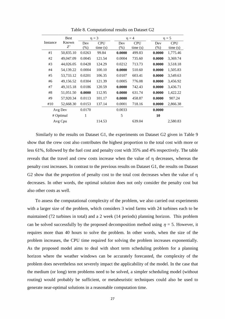
Table 8. Computational results on Dataset G2

Instance Best

Known Z’

η = 3 η = 4 η = 5 Dev (%)

CPU time (s)

Dev (%)

CPU time (s)

Dev (%)

CPU time (s)

#1 50,835.10 0.0263 99.84 0.0000 499.83 0.0000 1,775.46 #2 49,047.09 0.0045 121.54 0.0004 735.60 0.0000 3,369.74 #3 44,026.05 0.0428 124.29 0.0212 713.73 0.0000 3,518.18 #4 54,139.22 0.0004 100.10 0.0000 510.60 0.0000 1,505.83 #5 53,733.12 0.0201 106.35 0.0107 603.41 0.0000 3,549.63 #6 49,156.52 0.0304 121.39 0.0005 776.08 0.0000 3,456.92 #7 49,315.18 0.0186 120.59 0.0000 742.43 0.0000 3,436.71 #8 51,051.50 0.0000 112.95 0.0000 631.74 0.0000 1,422.22 #9 57,920.34 0.0113 101.17 0.0000 458.87 0.0000 907.24

#10 52,668.30 0.0153 137.14 0.0001 718.16 0.0000 2,866.38 Avg Dev 0.0170 0.0033 0.0000 # Optimal 1 5 10 Avg Cpu 114.53 639.04 2,580.83

Similarly to the results on Dataset G1, the experiments on Dataset G2 given in Table 9

show that the crew cost also contributes the highest proportion to the total cost with more or

less 61%, followed by the fuel cost and penalty cost with 35% and 4% respectively. The table

reveals that the travel and crew costs increase when the value of η decreases, whereas the

penalty cost increases. In contrast to the previous results on Dataset G1, the results on Dataset

G2 show that the proportion of penalty cost to the total cost decreases when the value of η

decreases. In other words, the optimal solution does not only consider the penalty cost but

also other costs as well.

To assess the computational complexity of the problem, we also carried out experiments

with a larger size of the problem, which considers 3 wind farms with 24 turbines each to be

maintained (72 turbines in total) and a 2 week (14 periods) planning horizon. This problem

can be solved successfully by the proposed decomposition method using η = 5. However, it

requires more than 40 hours to solve the problem. In other words, when the size of the

problem increases, the CPU time required for solving the problem increases exponentially.

As the proposed model aims to deal with short term scheduling problem for a planning

horizon where the weather windows can be accurately forecasted, the complexity of the

problem does nevertheless not severely impact the applicability of the model. In the case that

the medium (or long) term problems need to be solved, a simpler scheduling model (without

routing) would probably be sufficient, or metaheuristic techniques could also be used to

generate near-optimal solutions in a reasonable computation time.

27

Table 9. Cost breakdown for the solutions attained by the proposed method on Dataset G2

Instance

η = 3

η = 4

η = 5

Fuel Cost Crew Cost

Penalty Cost

Total Cost

Fuel Cost Crew Cost

Penalty Cost

Total Cost

Fuel Cost Crew Cost

Penalty Cost

Total Cost

#1 19,794.83 30,975.00 1,400.00 52,169.83

18,810.10 30,625.00 1,400.00 50,835.10

18,810.10 30,625.00 1,400.00 50,835.10

#2 17,045.11 32,225.00 0.00 49,270.11

17,114.72 31,950.00 0.00 49,064.72

16,702.09 30,975.00 1,370.00 49,047.09

#3 16,434.87 29,475.00 0.00 45,909.87

16,259.72 28,700.00 0.00 44,959.72

15,601.05 28,425.00 0.00 44,026.05

#4 18,834.46 33,450.00 1,876.00 54,160.46

18,813.22 33,450.00 1,876.00 54,139.22

18,813.22 33,450.00 1,876.00 54,139.22

#5 17,153.23 35,050.00 2,608.00 54,811.23

17,758.00 34,725.00 1,825.00 54,308.00

17,147.12 33,750.00 2,836.00 53,733.12

#6 19,354.96 29,875.00 1,420.00 50,649.96

18,512.57 29,250.00 1,420.00 49,182.57

18,461.52 29,275.00 1,420.00 49,156.52

#7 18,672.19 30,000.00 1,561.00 50,233.19

18,704.18 29,050.00 1,561.00 49,315.18

18,704.18 29,050.00 1,561.00 49,315.18

#8 17,667.50 29,825.00 3,559.00 51,051.50

17,667.50 29,825.00 3,559.00 51,051.50

17,667.50 29,825.00 3,559.00 51,051.50

#9 18,490.45 36,475.00 3,609.00 58,574.45

18,536.34 35,775.00 3,609.00 57,920.34

18,536.34 35,775.00 3,609.00 57,920.34

#10 18,166.46 32,125.00 3,183.00 53,474.46

17,694.28 30,800.00 4,180.00 52,674.28

17,988.30 30,500.00 4,180.00 52,668.30

Avg 18,161.41 31,947.50 1,921.60 52,030.51

17,987.06 31,415.00 1,943.00 51,345.06

17,843.14 31,165.00 2,181.10 51,189.24

Prop. 34.91 61.40 3.69 35.03 61.18 3.78 34.86 60.88 4.26

28

5.3 Comparative analysis: multiple wind farms and O&M bases model versus

single wind farm and O&M base model

In this subsection, the potential cost saving attained by implementing the multiple wind

farms and O&M bases model (referred to as the multiple model) instead of applying single

wind farm and O&M model separately (referred to as the single model) is presented. In the

single model, an O&M base is dedicated to serve only one wind farm. In other words, the

resources (vessels and technicians) are also only allocated to the corresponding wind farm.

Additional experiments were carried out to calculate the cost saving made by implementing

the multiple model. Dataset G1 is used in this experiment with a little amendment. We

increase the duration of weather windows for vessel V3 given in Table 4 for periods 1 and 2

from 7 hours to 12 hours. This is to increase the chance that the feasible optimal solution can

be obtained if the model is solved separately for each single model.

Table 10 presents the dataset configuration when the model is solved separately for each

single model. As Dataset G1 includes three wind farms and two O&M bases, we divide OM2

into two O&M bases namely OM2a and OM2b. OM1 only serves wind farm 1 (WF1)

whereas OM2a and OM2b are allocated to WF2 and WF3 respectively. The table also shows

that OM1 has two vessels while OM2a and OM2b have only one vessel. The number of

technicians for each skill type available in OM2a and OM2b is half of the one in OM2 (i.e. 6

technicians). The weather window for each vessel and each period is also given in Table 10.

As the model will be solved separately, there are three single problems that need to be

addressed with the total cost calculated by summing up the cost obtained from each problem.

Ten instances (sets of turbines) of Dataset G1 are also used in this experiment.

Table 10. Dataset configuration for single wind farm and O&M base model

O&M Number of Technicians Wind

farm Vessel Weather Window (hours)

Type 1 Type 2 Type 3 Period 1 Period 2 Period 3

OM1 6 6 6 WF1 V1 6 6 12 V2 12 12 12

OM2a 3 3 3 WF2 V3 12 12 12 OM2b 3 3 3 WF3 V4 12 12 12

Table 11 shows the comparative analysis between multiple and single models, where the

objective function value (total cost), CPU time (in seconds), and %Dev (deviation from the

results of the single model to the multiple ones) are given.

29

Table 11. Comparison of results between the multiple and single models

Instance

multiple model

single model

Saving

OM1 serves WF 1

OM2a serves WF 2

OM2b serves WF 3

Total Solution

(OM1+OM2a+OM2b)

Z CPU

time (s) Z

CPU time (s)

Z CPU

time (s) Z

CPU time (s)

Z CPU

time (s) Cost %Dev

#1 35,944.17 718.78

12,683.69 144.34

10,559.94 3.61

16,055.94 11.84

39,299.57 159.80

3,355.40 9.34

#2 31,378.89 258.85

10,000.42 103.18

13,600.63 2.32

12,033.73 6.53

35,634.78 112.03

4,255.89 13.56

#3 32,680.80 183.13

12,380.20 42.73

NF -

11,408.92 13.17

NF -

NF -

#4 28,770.38 579.89

9,592.68 331.37

8,986.75 8.52

15,385.18 4.10

33,964.61 344.00

5,194.23 18.05

#5 28,068.42 249.75

10,178.69 110.29

9,290.87 3.23

10,572.14 4.77

30,041.69 118.29

1,973.28 7.03

#6 33,795.43 134.31

11,822.31 30.57

NF -

NF -

NF -

NF -

#7 27,499.47 559.84

9,909.68 125.52

9,040.84 9.08

10,476.79 30.87

29,427.31 165.47

1,927.84 7.01

#8 32,036.04 254.39

12,412.67 21.34

8,398.74 2.71

14,480.66 7.03

35,292.07 31.08

3,256.03 10.16

#9 27,392.17 797.20

9,140.52 51.76

11,061.70 2.75

12,758.18 33.94

32,960.40 88.45

5,568.22 20.33

#10 30,517.21 286.07

8,807.03 157.27

NF -

12,637.36 5.33

NF -

NF -

Average 488.39

145.59

12.21

30

In this experiment we set the maximum number of turbines that can be visited by a vessel (η)

to 5 as this value provides the optimal solutions for the multiple model. In Table 11, the

solutions for each single problem along with total solution for all single problems are

provided. The table shows that in instances 3, 6, and 10 the feasible solution cannot be

obtained (infeasible solution – NF) when the problem is solved separately. This is due to the

lack of resources needed in an O&M base to serve an offshore wind farm. This disadvantage

can be overcome by implementing the multiple model where feasible optimal solutions can

be obtained by sharing resources to maintain wind turbine in several wind farms. Table 11

also reveals that implementing the multiple model instead of the single model separately will

also reduce the maintenance cost by 12.21% on average (calculated based on the results with

feasible solutions). However, the computational time (on average) needed to solve the

multiple model is more than three times compared to the one to solve all single problems.

This is due to the fact that the number of possible routes for a vessel for visiting wind

turbines in the multiple model is higher than in the single model.

6. Conclusion and suggestions

In this paper, we propose an optimisation model and a decomposition solution method

for maintenance routing and scheduling in offshore wind farms. A mathematical model for

selecting the optimum route configuration is developed to minimise the total cost comprising

travel, technicians, and penalty costs. An algorithm incorporating a MILP model for

generating all feasible routes is also proposed. The algorithm explores all combinations of

turbines that are feasible to be serviced in a period and finds the optimal routing for the

vessels to visit those turbines.

The proposed approach was tested on two types of datasets. The first one is the existing

dataset from the literature provided by Dai et al. (2015), whereas the second one is randomly

generated. The computational experiments on the existing dataset show that the proposed

approach outperforms the method proposed by Dai et al. (2015). The proposed method

obtained the optimal solutions in a relatively small computational time. The new datasets are

generated for evaluating the proposed method to solve the enhanced model where multiple

wind farms, multiple O&M bases, and the number of each technician type available at each

O&M base are considered. The newly generated dataset is relatively hard to solve, and based

on computational experiments, the proposed method required more time to obtain the optimal

31

solutions on this dataset than on the less challenging data set of Dai et al. (2015). Additional

experiments are also carried out to assess the advantage of implementing the model for

multiple wind farms and O&M bases compared to the model for single wind farm and O&M

base. Based on the computational experiments, the proposed model (for multiple wind farms

and O&M bases) not only gives a cost saving of 12.21% on average, but also provides

optimal feasible solutions when the feasible solution cannot be found in the single problem

(one wind farm and one O&M base) due to lack of resources (vessels and technicians).

There are a number of possible extensions to enhance the model to make it more

applicable to both offshore wind farms in operation and under development. For larger wind

farms and clusters of wind farms, one could investigate metaheuristic techniques to solve

relatively larger maintenance routing and scheduling problems. For far-offshore wind farms

and clusters of these, the scheduling and routing of Service Operation Vessels (SOV) or other

"mother vessels" staying offshore for multiple days becomes more relevant. One challenge is

coordinating the operation of such vessels with the use of daughter vessels, ordinary CTVs

and possibly also helicopters. Another logistics solution for far-offshore wind farms, namely

offshore accommodation platforms serving one or a cluster of wind farms, can on the other

hand be represented in the proposed model without the need for any extensions. Extended or

similar models could also include possible safety constraints specific to the offshore logistics

for a given offshore wind farm. Furthermore, the model could also be extended to include the

grouping of the maintenance tasks and number of turbine visits as decision variables, thus

allowing "opportunistic" maintenance scheduling and an even more efficient utilization of the

resources. Including revenue losses in the penalty costs to penalize preventive maintenance

during good wind conditions would also be a promising extension of the model to further

improve the maintenance schedule.

One major challenge for application as an operational decision support tool for a real

offshore wind farm is the uncertainty and variability associated with weather conditions.

Stochastic constraints such as weather condition uncertainty could also be taken into account

in the model. Considering also the experience of the CTV crew on the local conditions within

the wind farm could also improve the applicability of this optimisation model.

32

Acknowledgments

The research leading to these results has received funding from the European Union Seventh Framework

Programme under the agreement SCP2-GA-2013-614020 (LEANWIND: Logistic Efficiencies And Naval

architecture for Wind Installations with Novel Developments).

References

1. Baldacci, R., Bartolini, E., Mingozzi, A. (2011). An exact algorithm for the pickup and delivery problem with time windows. Operations Research, 59, 414-426.

2. Barnhart, C., Johnson, E.L., Nemhauser, G.L., Savelsbergh, M.V.P., Vance, P.H. (1998). Column generation for solving huge integer programs. Operations Research 46(3). 316-329.

3. Berbeglia, G., Cordeau, J-F., Gribkovskaia, I., Laporte, G. (2007). Static pickup and delivery problems: a classification scheme and survey. TOP, 15, 1-31.

4. Besnard, F., Patriksson, M., Strőmberg, A., Wojciechowski, A., Bertling, L. (2009). An Optimization Framework for Opportunistic Maintenance of Offshore Wind Power System. In Proceedings of IEEE Bucharest Powertech Conference. Bucharest, Romania.

5. Besnard, F., Patriksson, M., Strőmberg, A., Wojciechowski, A., Bertling, L. (2011). A stochastic model for opportunistic service maintenance planning of offshore wind farms. In: Proceedings of the IEEE Powertech Conference. Trondheim, Norway.

6. Bjelić, N., Vidović, M., Popović, D. (2013). Variable neighborhood search algorithm for heterogeneous traveling repairmen problem with time windows. Expert Systems with Applications, 40, 5997–6006.

7. Bock, S. (2015). Solving the traveling repairman problem on a line with general processing times and deadlines. European Journal of Operational Research, 244, 690 - 703.

8. Brønmo, G., Nygreen, B., Lysgaard, J. (2010). Column generation approaches to ship routing and scheduling with flexible cargo sizes. European Journal of Operational Research, 200, 139-150.

9. Byon, E., Pérez, E., Ding, Y, Ntaimo, L. (2011). Simulation of wind farm operations and maintenance using discrete event system specification. Simulation, 87, 1093-1117.

10. Camci, F. (2014). The travelling maintainer problem: integration of condition-based maintenance with the travelling salesman problem. Journal of the Operational Research Society, 65, 1423–1436.

33

11. Camci, F. (2015). Maintenance scheduling of geographically distributed assets with prognostics information. European Journal of Operational Research, 245, 506-516.

12. Cordeau, J-F., Laporte, G. (2007). The dial-a-ride problem: models and algorithms. Annals of Operations Research 153, 29-46.

13. Dantzig, G.B., Wolfe, P. (1960). Decomposition principle for linear programs. Operations Research 8, 101-111.

14. Dumas, Y., Desrosiers, J., Soumis, F. (1991). The pickup and delivery problem with time windows. European Journal of Operational Research, 54 (1), 7-22.

15. Dai, L., Stålhane, M. Utne, I.B. (2015). Routing and scheduling of maintenance fleet for offshore wind farms. Wind Engineering, 39, 15–30.

16. Dewilde, T., Cattrysse, D., Coene, S., Spieksma, F.C.R., Vansteenwegen, P. (2013). Heuristics for the traveling repairman problem with profits. Computers & Operations Research, 40, 1700 - 1707.

17. European Committee for Standardization (2010). Maintenance: Maintenance terminology. EN 13306: 2010.

18. García-González, J., delaMuela, R.M.R., Santos, L.M., Gonzalez, A.M. (2008). Stochastic joint optimization of wind generation and pumped-storage units in an electricity market. IEEE Transactions on Power Systems, 23, 460-468.

19. Gschwind, T. (2015) A comparison of column-generation approaches to the Synchronized Pickup and Delivery Problem. European Journal of Operational Research, 247(1), 60-71.

20. Kovács, A., Erdős, G., Viharos, Z.J., Monostori, L. (2011). A system for the detailed scheduling of wind farm maintenance. CIRP Annals Manufacturing Technology, 60, 497-501.

21. Luo, Z., Qin, H., Lim, A. (2014). Branch-and-price-and-cut for the multiple traveling repairman problem with distance constraints. European Journal of Operational Research, 234, 49–60.

22. Parikh, N.D. (2012). Optimizing maintenance cost of wind farms by scheduling preventive maintenance and replacement of critical components using mathematical approach. Master thesis. Texas A&M University, US.

23. Parragh, S. N., Pinho de Sousa, J., Almada-Lobo, B. (2015) The Dial-a-Ride Problem with Split Requests and Profits. Transportations Science 49(2), p. 311-334.

24. Perez-Canton, S., Rubio-Romero, J.C. (2013). A model for the preventive maintenance scheduling of power plants including wind farms. Reliability Engineering & System Safety, 119, 67-75.

34

25. Poggi, M., Uchoa, E. (2014). New Exact Algorithms for the Capacitated Vehicle Routing Problem. In: Toth, P., Vigo, D. (Eds.), Vehicle Routing Problems, Methods, and Applications, 2nd Edition. SIAM, p. 59-86

26. Røpke, S., Cordeau, J-F. (2009). Branch-and-cut-and-price for the pickup and delivery problem with time windows. Transportation Science 43 (3), 267-286.

27. Salehipour, A., Sörensen, K., Goos, P., Bräysy, O. (2011). Efficient GRASP+VND and GRASP+VNS metaheuristics for the traveling repairman problem. 4Q Journal of Operations Research, 9, 189–209.

28. Savelsbergh, M., Sol, M. (1998). Drive: Dynamic Routing of Independent Vehicles. Operations Research, 46 (4), 474-490.

29. Shafiee, M. (2015). Maintenance logistics organization for offshore wind energy: Current progress and future perspectives. Renewable Energy, 77, 182-193.

30. Snyder, B., Kaiser, M., (2009). Ecological and economic cost-benefit analysis of offshore wind energy. Renewable Energy 34 (6), 1567–1578.

31. Stålhane, M., Hvattum, L.M., Skaar. (2015). Optimization of routing and scheduling of vessels to perform maintenance at offshore wind farms. Energy Procedia, 80, 92-99.

32. Van Horenbeek, A., Van Ostaeyen, J., Duflou, J., Pintelon, L. (2012). Prognostic maintenance scheduling for offshore wind turbine farms. In Proceedings of the 4th Production & Operations Management World Conference. Amsterdam, the Netherlands.

33. Zhang, J., Chowdhury, S., Zhang, J. (2012). Optimal preventive maintenance time windows for offshore wind farms subject to wake losses. In Proceedings of the 14th AIAA/ISSMO Multidisciplinary Analysis and Optimization Conference. Indianapolis, US.

34. Zhang, Z., Kusiak, A., Song, Z. (2013). Scheduling Electric Power Production at a Wind Farm. European Journal of Operational Research, 224, 227-238.

35