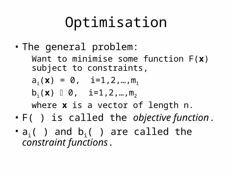
Optimisation

• The general problem:Want to minimise some function F(x) subject to constraints,

ai(x) = 0, i=1,2,…,m1

bi(x) 0, i=1,2,…,m2

where x is a vector of length n.

• F( ) is called the objective function.• ai( ) and bi( ) are called the constraint

functions.

Special Cases

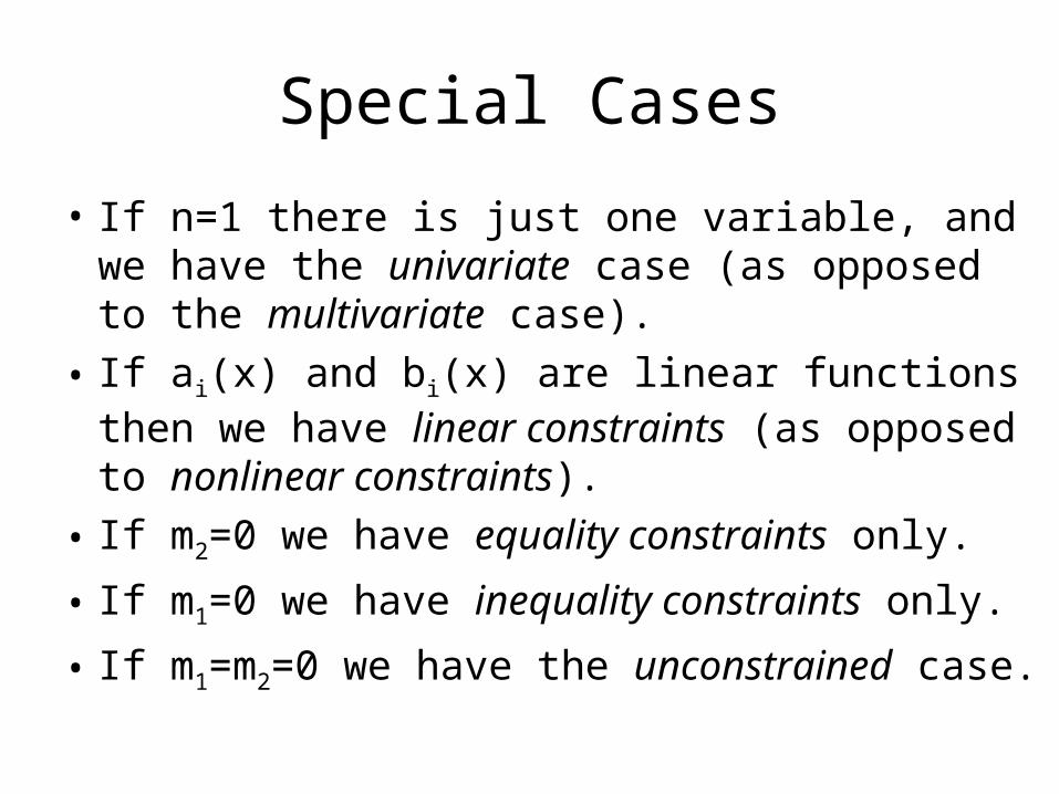
• If n=1 there is just one variable, and we have the univariate case (as opposed to the multivariate case).

• If ai(x) and bi(x) are linear functions then we have linear constraints (as opposed to nonlinear constraints).

• If m2=0 we have equality constraints only.

• If m1=0 we have inequality constraints only.

• If m1=m2=0 we have the unconstrained case.

Techniques

• The techniques used to solve an optimisation problem depends on the properties of the functions F, ai, and bi.

• Important factors include:– Univariate or multivariate case?– Constrained or unconstrained problem?– Do we know the derivatives of F?

Example Linear Problem• An oil refinery can buy light crude at £35/barrel and

heavy crude at £30/barrel. • Refining one barrel of oil produces petrol, heating oil,

and jet fuel as follows:

Petrol Heating oil Jet fuel

Light crude 0.3 0.2 0.3

Heavy crude 0.3 0.4 0.2

• The refinery has contracts for 0.9M barrels of petrol, 0.8M barrels of heating oil and 0.5M barrels of jet fuel.

• How much light and heavy crude should the refinery buy to satisfy the contracts at least cost?

Problem Specification

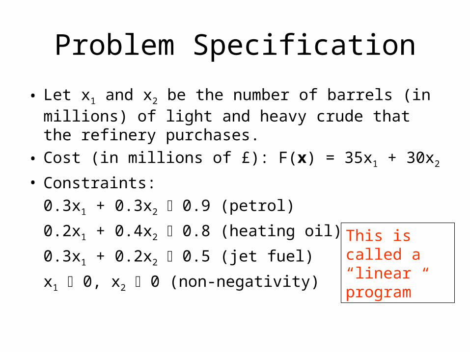
• Let x1 and x2 be the number of barrels (in millions) of light and heavy crude that the refinery purchases.

• Cost (in millions of £): F(x) = 35x1 + 30x2

• Constraints:

0.3x1 + 0.3x2 0.9 (petrol)

0.2x1 + 0.4x2 0.8 (heating oil)

0.3x1 + 0.2x2 0.5 (jet fuel)

x1 0, x2 0 (non-negativity)

This is called a “linear program”

Graphical Solution

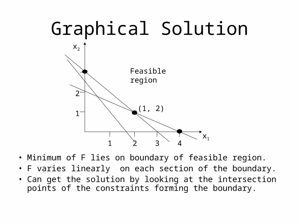
• Minimum of F lies on boundary of feasible region.• F varies linearly on each section of the boundary.• Can get the solution by looking at the intersection points

of the constraints forming the boundary.

Feasible region

x2

x14321

1

2

(1, 2)

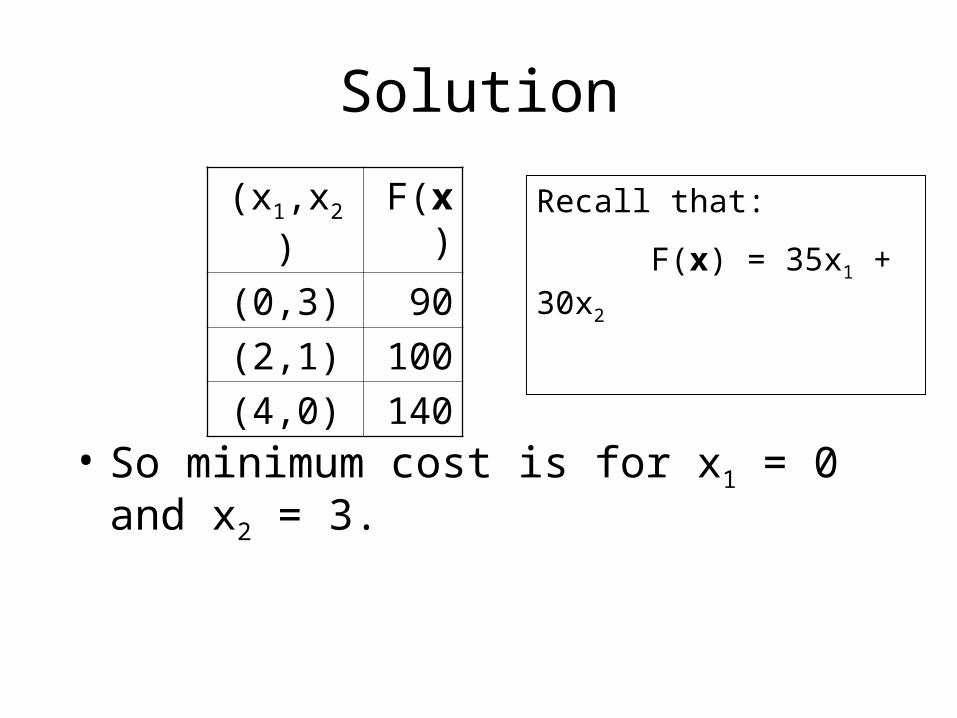
Solution

(x1,x2) F(x)

(0,3) 90

(2,1) 100

(4,0) 140

• So minimum cost is for x1 = 0 and x2 = 3.

Recall that:

F(x) = 35x1 + 30x2

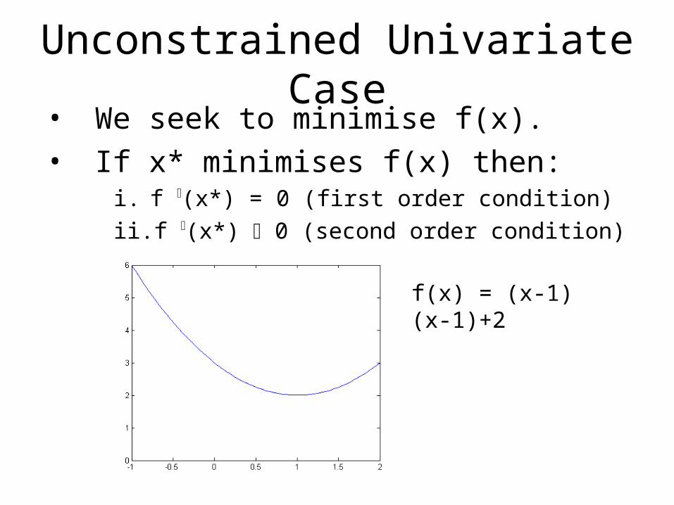
Unconstrained Univariate Case• We seek to minimise f(x).

• If x* minimises f(x) then:i. f (x*) = 0 (first order condition)

ii. f (x*) 0 (second order condition)

f(x) = (x-1)(x-1)+2

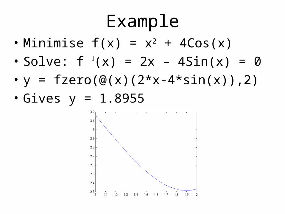
Example• Minimise f(x) = x2 + 4Cos(x)

• Solve: f (x) = 2x – 4Sin(x) = 0

• y = fzero(@(x)(2*x-4*sin(x)),2)

• Gives y = 1.8955

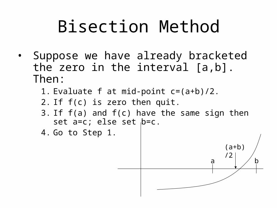
Bisection Method

• Suppose we have already bracketed the zero in the interval [a,b]. Then:

1. Evaluate f at mid-point c=(a+b)/2.2. If f(c) is zero then quit.3. If f(a) and f(c) have the same sign then set a=c;

else set b=c.4. Go to Step 1.

a b

(a+b)/2

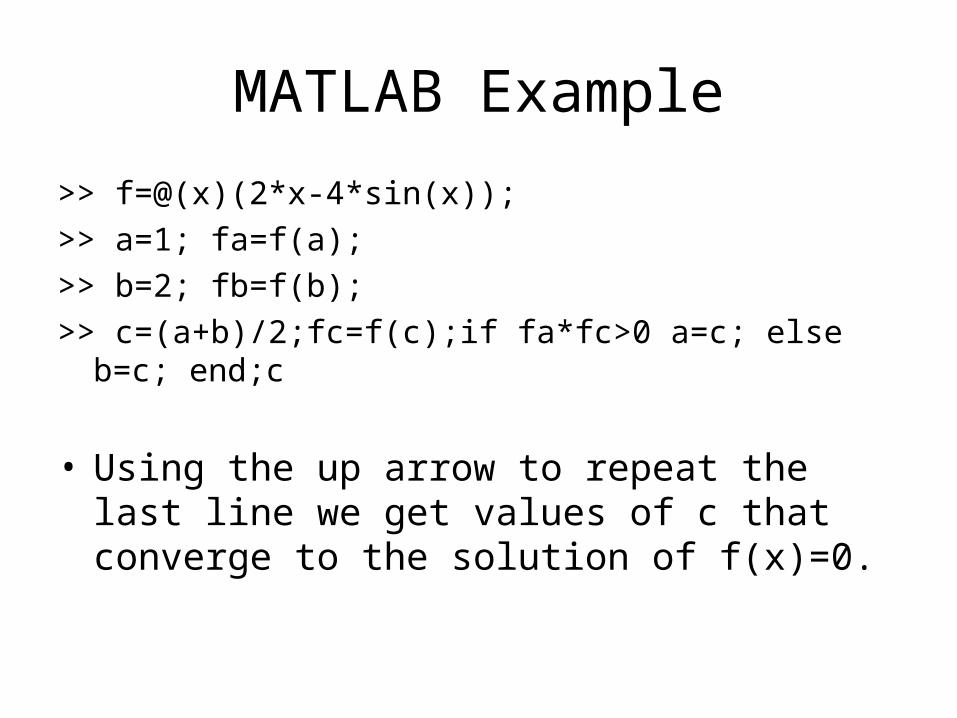
MATLAB Example

>> f=@(x)(2*x-4*sin(x));

>> a=1; fa=f(a);

>> b=2; fb=f(b);

>> c=(a+b)/2;fc=f(c);if fa*fc>0 a=c; else b=c; end;c

• Using the up arrow to repeat the last line we get values of c that converge to the solution of f(x)=0.

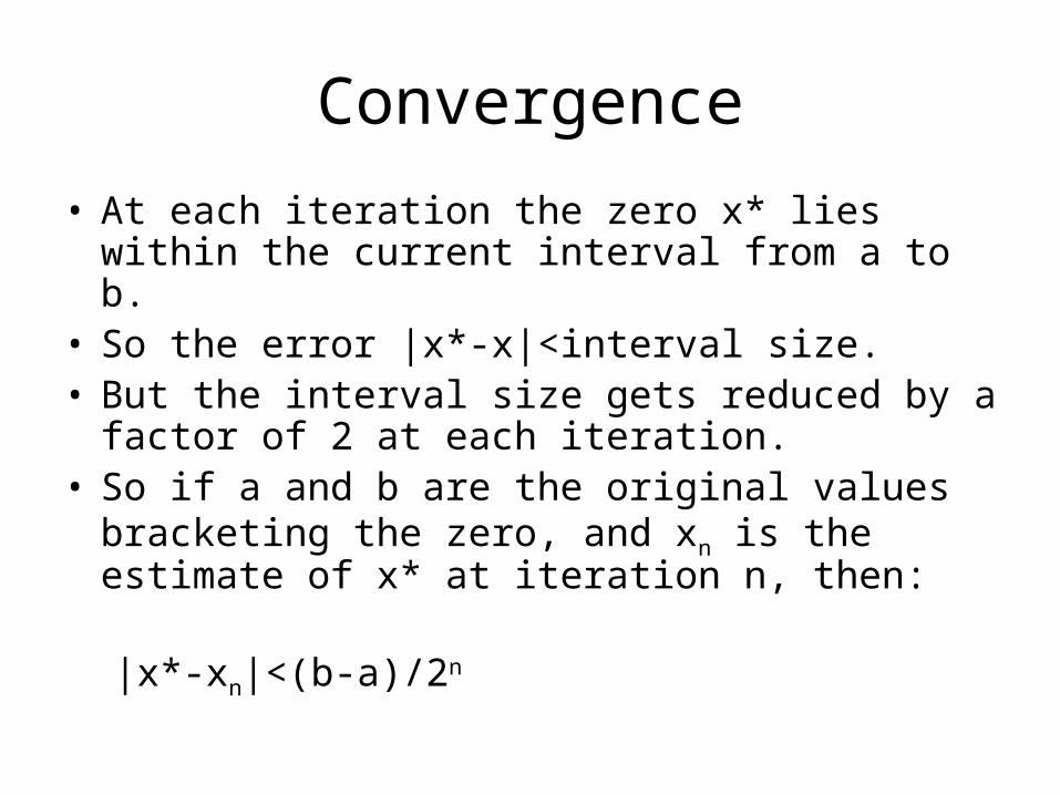
Convergence

• At each iteration the zero x* lies within the current interval from a to b.

• So the error |x*-x|<interval size.• But the interval size gets reduced by a factor of

2 at each iteration.• So if a and b are the original values bracketing

the zero, and xn is the estimate of x* at iteration n, then:

|x*-xn|<(b-a)/2n

f(xk)

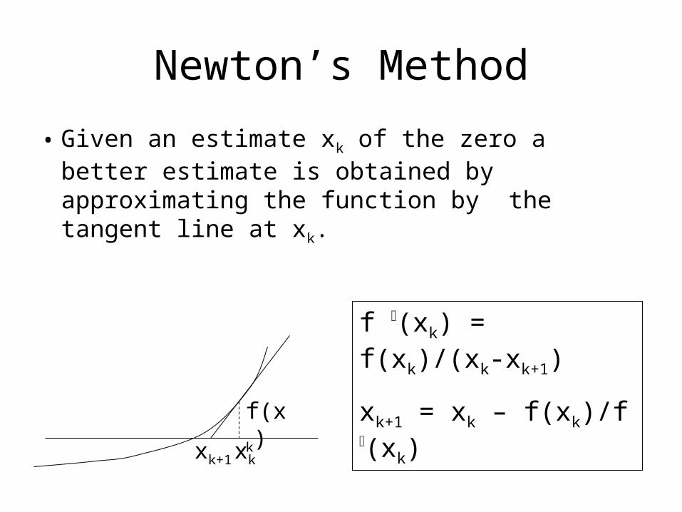
Newton’s Method

• Given an estimate xk of the zero a better estimate is obtained by approximating the function by the tangent line at xk.

xkxk+1

f (xk) = f(xk)/(xk-xk+1)

xk+1 = xk – f(xk)/f (xk)

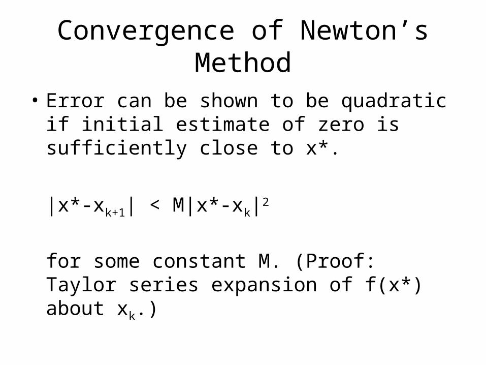
Convergence of Newton’s Method

• Error can be shown to be quadratic if initial estimate of zero is sufficiently close to x*.

|x*-xk+1| < M|x*-xk|2

for some constant M. (Proof: Taylor series expansion of f(x*) about xk.)

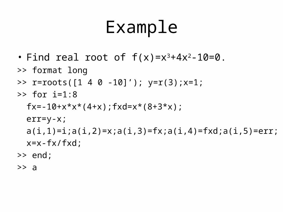
Example

• Find real root of f(x)=x3+4x2-10=0.>> format long

>> r=roots([1 4 0 -10]’); y=r(3);x=1;

>> for i=1:8

fx=-10+x*x*(4+x);fxd=x*(8+3*x);

err=y-x;

a(i,1)=i;a(i,2)=x;a(i,3)=fx;a(i,4)=fxd;a(i,5)=err;

x=x-fx/fxd;

>> end;

>> a

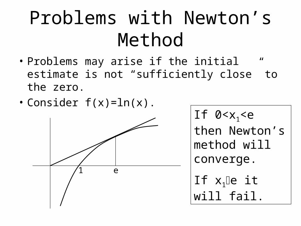
Problems with Newton’s Method

• Problems may arise if the initial estimate is not “sufficiently close” to the zero.

• Consider f(x)=ln(x).

e1

If 0<x1<e then Newton’s method will converge.

If x1e it will fail.

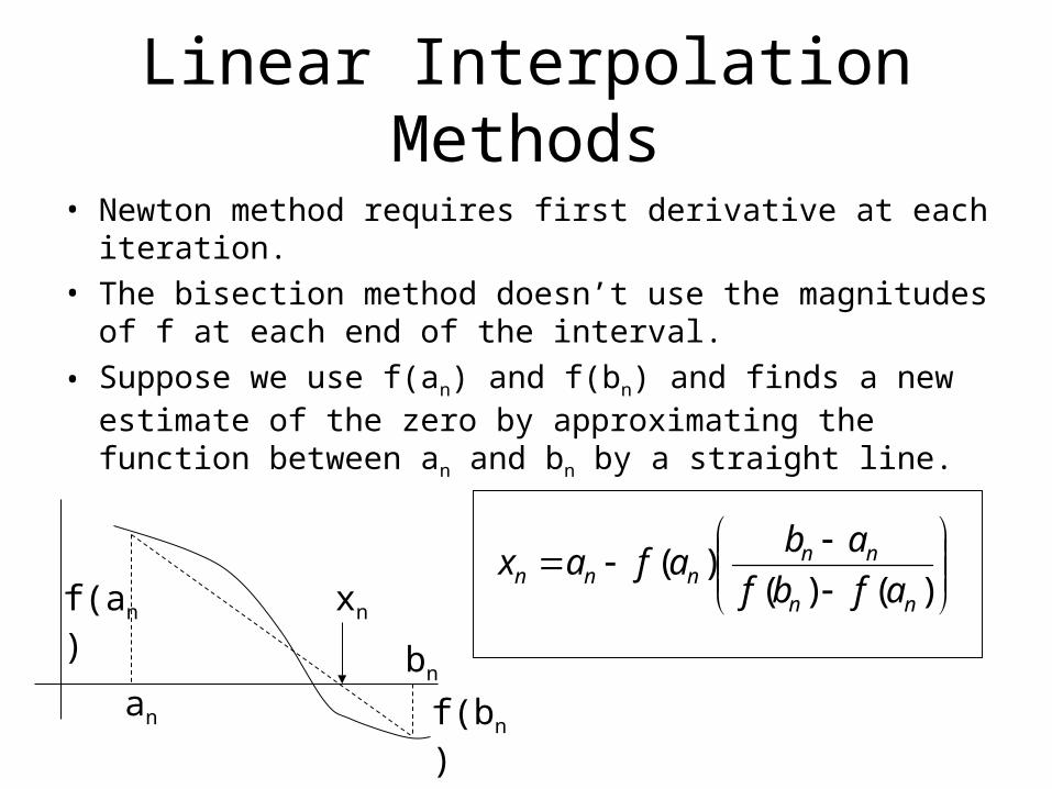
Linear Interpolation Methods

• Newton method requires first derivative at each iteration.• The bisection method doesn’t use the magnitudes of f at

each end of the interval.

• Suppose we use f(an) and f(bn) and finds a new estimate of the zero by approximating the function between an and bn by a straight line.

f(bn)

bn

an

xnf(an)

)()(

)(nn

nnnnn afbf

abafax

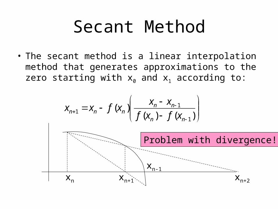
Secant Method

• The secant method is a linear interpolation method that generates approximations to the zero starting with x0 and x1 according to:

)()(

)(1

11

nn

nnnnn xfxf

xxxfxx

xn-1

xn xn+1 xn+2

Problem with divergence!

Method of False Position

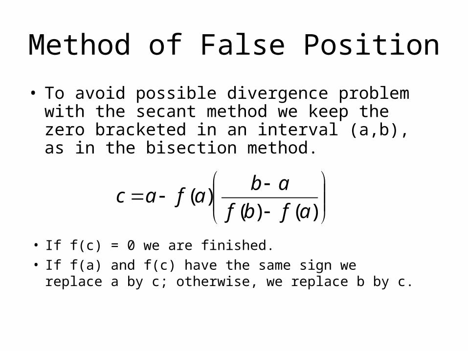
• To avoid possible divergence problem with the secant method we keep the zero bracketed in an interval (a,b), as in the bisection method.

)()(

)(afbf

abafac

• If f(c) = 0 we are finished.• If f(a) and f(c) have the same sign we replace

a by c; otherwise, we replace b by c.

Golden Section Method

• A function is unimodal on an interval [a,b] if it has a single local minimum on [a,b].

• The Golden Section method can be used to find the minimum of function F on [a,b], where F is unimodal on [a,b].

• This method is not based on solving F(x)=0.

• We seek to avoid unnecessary function evaluations.

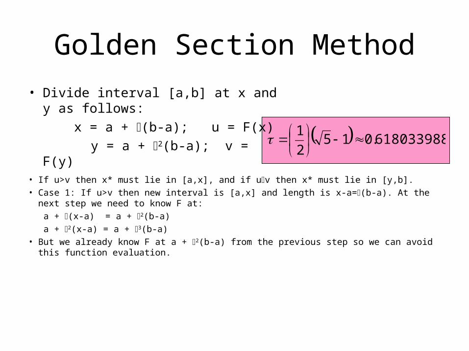
• If u>v then x* must lie in [a,x], and if uv then x* must lie in [y,b].• Case 1: If u>v then new interval is [a,x] and length is x-a=(b-a). At the next step we need to know

F at:

a + (x-a) = a + 2(b-a)

a + 2(x-a) = a + 3(b-a)• But we already know F at a + 2(b-a) from the previous step so we can avoid this function

evaluation.

Golden Section Method

• Divide interval [a,b] at x and y as follows:

x = a + (b-a); u = F(x)

y = a + 2(b-a); v = F(y) 6180339887.015

2

1

Golden Section Method

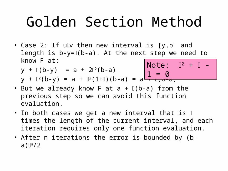
• Case 2: If uv then new interval is [y,b] and length is b-y=(b-a). At the next step we need to know F at:

y + (b-y) = a + 22(b-a)

y + 2(b-y) = a + 2(1+)(b-a) = a + (b-a)• But we already know F at a + (b-a) from the previous

step so we can avoid this function evaluation.• In both cases we get a new interval that is times the

length of the current interval, and each iteration requires only one function evaluation.

• After n iterations the error is bounded by (b-a)n/2

Note: 2 + - 1 = 0

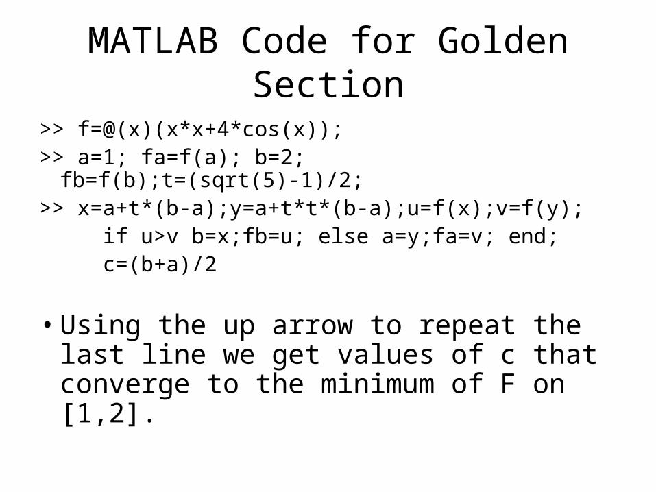
MATLAB Code for Golden Section

>> f=@(x)(x*x+4*cos(x));>> a=1; fa=f(a); b=2; fb=f(b);t=(sqrt(5)-1)/2;>> x=a+t*(b-a);y=a+t*t*(b-a);u=f(x);v=f(y); if u>v b=x;fb=u; else a=y;fa=v; end; c=(b+a)/2

• Using the up arrow to repeat the last line we get values of c that converge to the minimum of F on [1,2].