Optimization Algorithms for Analyzing Large Datasets

Optimization Algorithms for Analyzing Large Datasets

Stephen Wright

University of Wisconsin-Madison

Winedale, October, 2012

Stephen Wright (UW-Madison) Optimization Winedale, October, 2012 1 / 67

1 Learning from Data: Problems and Optimization Formulations

2 First-Order Methods

3 Stochastic Gradient Methods

4 Nonconvex Stochastic Gradient

5 Sparse / Regularized Optimization

6 Decomposition / Coordinate Relaxation

7 Lagrangian Methods

8 Higher-Order Methods


Outline

Give some examples of data analysis and learning problems and theirformulations as optimization problems.

Highlight common features in these formulations.

Survey a number of optimization techniques that are being applied tothese problems.

Just the basics - give the flavor of each method and state a keytheoretical result or two.

All of these approaches are being investigated at present; rapiddevelopments continue.


Data Analysis: Learning

Typical ingredients of optimization formulations of data analysis problems:

Collection of data, from which we want to learn to make inferencesabout future / missing data, or do regression to extract keyinformation.

A model of how the data relates to the meaining we are trying toextract. Model parameters to be determined by inspecting the dataand using prior knowledge.

Objective that captures prediction errors on the data and deviationfrom prior knowledge or desirable structure.

Other typical properties of learning problems are huge underlying data set,and requirement for solutions with only low-medium accuracy.

In some cases, the optimization formulation is well settled. (e.g. LeastSquares, Robust Regression, Support Vector Machines, LogisticRegression, Recommender Systems.)

In other areas, formulation is a matter of ongoing debate!Stephen Wright (UW-Madison) Optimization Winedale, October, 2012 4 / 67

LASSO

Least Squares: Given a set of feature vectors ai ∈ Rn and outcomes bi ,i = 1, 2, . . . ,m, find weights x on the features that predict the outcomeaccurately: aTi x ≈ bi .

Under certain assumptions on measurement error, can find a suitable x bysolving a least squares problem

minx

1

2‖Ax − b‖2

2,

where the rows of A are aTi , i = 1, 2, . . . ,m.

Suppose we want to identify the most important features of each ai —those features most important in predicting the outcome.

In other words, we seek an approx least-squares solution x that is sparse— and x with just a few nonzero components. Obtain

LASSO: minx

1

2‖Ax − b‖2

2 such that ‖x‖1 ≤ T ,

for parameter T > 0. (Smaller T implies fewer nonzeros in x .)Stephen Wright (UW-Madison) Optimization Winedale, October, 2012 5 / 67

LASSO and Compressed Sensing

LASSO is equivalent to an “`2-`1” formulation:

minx

1

2‖Ax − b‖2

2 + τ‖x‖1, for some τ > 0.

This same formulation is common in compressed sensing, but themotivation is slightly different. Here x represents some signal that isknown to be (nearly) sparse, and the rows of A are probing x to givemeasured outcomes b. The problem above is solved to reconstruct x .


Group LASSO

Partition x into groups of variables that have some relationship — turnthem “on” or “off” as a group, not as individuals.

minx

1

2‖Ax − b‖2

2 + τ∑g∈G‖x[g ]‖2,

with each [g ] ⊂ 1, 2, . . . , n.Easy handle when groups [g ] are disjoint.

Still easy when ‖ · ‖2 is replaced by ‖ · ‖∞. (Turlach, Venables,Wright, 2005)

When the groups form a hierarchy, the problem is slightly harder butsimilar algorithms still work.

For general overlapping groups, algorithms are more complex (seeBach, Mairal, et al.)


Least Squares with Nonconvex Regularizers

Nonconvex element-wise penalties have become popular for variableselection in statistics.

SCAD (smoothed clipped absolute deviation) (Fan and Li, 2001)

MCP (Zhang, 2010).

Properties: Unbiased and sparse estimates, solution path continuous inregularization parameter τ .

SparseNet (Mazumder, Friedman, Hastie, 2011): coordinate descent.Stephen Wright (UW-Madison) Optimization Winedale, October, 2012 8 / 67

Support Vector Classification

Given many data vectors xi ∈ Rn, for i = 1, 2, . . . ,m, together with a labelyi = ±1 to indicate the class (one of two) to which xi belongs.

Find z such that (usually) we have

xTi z ≥ 1 when yi = +1;

xTi z ≤ −1 when yi = −1.

SVM with hinge loss:

f (z) = CN∑i=1

max(1− yi (zT xi ), 0) +

1

2‖z‖2,

where C > 0 is a parameter. Dual formulation is

minα

1

2αTKα− 1Tα subject to 0 ≤ α ≤ C1, yTα = 0,

where Kij = yiyjxTi xj . Subvectors of the gradient Kα− 1 can be

computed economically.

(Many extensions and variants.)Stephen Wright (UW-Madison) Optimization Winedale, October, 2012 9 / 67

(Regularized) Logistic Regression

Seek odds function parametrized by z ∈ Rn:

p+(x ; z) := (1 + ezT x)−1, p−(x ; z) := 1− p+(z ;w),

choosing z so that p+(xi ; z) ≈ 1 when yi = +1 and p−(xi ; z) ≈ 1 whenyi = −1. Scaled, negative log likelihood function L(z) is

L(z) = − 1

m

∑yi=−1

log p−(xi ; z) +∑yi=1

log p+(xi ; z)

To get a sparse z (i.e. classify on the basis of a few features) solve:

minzL(z) + λ‖z‖1.


Multiclass Logistic Regression

M classes: yij = 1 if data point i is in class j ; yij = 0 otherwise. z[j] is thesubvector of z for class j .

f (z) = − 1

N

N∑i=1

M∑j=1

yij(zT[j]xi )− log(

M∑j=1

exp(zT[j]xi ))

+ λ

M∑j=1

‖z[j]‖22.

Useful in speech recognition, to classify phonemes.


Matrix Completion

Seek a matrix X ∈ Rm×n with low rank that matches certain observations,possibly noisy.

minX

1

2‖A(X )− b‖2

2 + τψ(X ),

where A(X ) is a linear mapping of the components of X (e.g.element-wise observations).

Can have ψ as the nuclear norm = sum of singular values. Tends topromote low rank (in the same way as ‖x‖1 tends to promote sparsity of avector x).

Alternatively: X is the sum of sparse matrix and a low-rank matrix. Theelement-wise 1-norm ‖X‖1 is useful in inducing sparsity.

Useful in recommender systems, e.g. Netflix, Amazon.


*~=


Image Processing: TV Regularization

Natural images are not random! They tend to have large areas ofnear-constant intensity or color, separated by sharp edges.

Denoising: Given an image in which the pixels contain noise, find a“nearby natural image.”

Total-Variation Regularization applies an `1 penalty to gradients in theimage.

u : Ω→ R, Ω := [0, 1]× [0, 1],

To denoise an image f : Ω→ R, solve

minu

∫Ω

(u(x)− f (x))2 dx + λ

∫Ω‖∇u(x)‖2

2 dx .

(Rudin, Osher, Fatemi, 1992)


(a) Cameraman: Clean (b) Cameraman: Noisy


(c) Cameraman: Denoised (d) Cameraman: Noisy


Optimization: Regularization Induces Structure

Formulations may include regularization functions to induce structure:

minx

f (x) + τψ(x),

where ψ induces the desired structure in x . Often ψ is nonsmooth.

‖x‖1 to induce sparsity in the vector x (variable selection / LASSO);

SCAD and MCP: nonconvex regularizers to induce sparsity, withoutbiasing the solution;

Group regularization / group selection;

Nuclear norm ‖X‖∗ (sum of singular values) to induce low rank inmatrix X ;

low “total-variation” in image processing;

generalizability (Vapnik: “...tradeoff between the quality of theapproximation of the given data and the complexity of theapproximating function”).


Optimization: Properties of f .

Objective f can be derived from Bayesian statistics + maximum likelihoodcriterion. Can incorporate prior knowledge.

f have distinctive properties in several applications:

Partially Separable: Typically

f (x) =1

m

m∑i=1

fi (x),

where each term fi corresponds to a single item of data, and possiblydepends on just a few components of x .

Cheap Partial Gradients: subvectors of the gradient ∇f may beavailable at proportionately lower cost than the full gradient.

These two properties are often combined.


Batch vs Incremental

Considering the partially separable form

f (x) =1

m

m∑i=1

fi (x),

the size N of the training set can be very large. There’s a fundamentaldivide in algorithmic strategy.

Incremental: Select a single i ∈ 1, 2, . . . ,m at random, evaluate∇fi (x), and take a step in this direction. (Note thatE [∇fi (x)] = ∇f (x).) Stochastic Approximation (SA) a.k.a.Stochastic Gradient (SG).

Batch: Select a subset of data X ⊂ 1, 2, . . . ,m, and minimize thefunction f (x) =

∑i∈X fi (x). Sample-Average Approximation (SAA).

Minibatch is a kind of compromise: Aggregate the component functionsfi into small groups, consisting of 10 or 100 individual terms, and applyincremental algorithms to the redefined summation. (Gives lower-variancegradient estimates.)


First-Order Methods

min f (x), with smooth convex f . First-order methods calculate ∇f (xk) ateach iteration, and do something with it.

Usually assumeµI ∇2f (x) LI for all x ,

with 0 ≤ µ ≤ L. (L is thus a Lipschitz constant on the gradient ∇f .)Function is strongly convex if µ > 0.

But some of these methods are extendible to more general cases, e.g.

nonsmooth-regularized f ;

simple constraints x ∈ Ω;

availability of just an approximation to ∇f .


Steepest Descent

xk+1 = xk − αk∇f (xk), for some αk > 0.

Choose step length αk by doing line search, or more simply by usingknowledge of L and µ.

αk ≡ 1/L yields sublinear convergence

f (xk)− f (x∗) ≤ 2L‖x0 − x∗‖2

k.

In strongly convex case, αk ≡ 2/(µ+ L) yields linear convergence, withconstant dependent on problem conditioning κ := L/µ:

f (xk)− f (x∗) ≤ L

2

(1− 2

κ+ 1

)2k

‖x0 − x∗‖2.

We can’t improve much on these rates by using more sophisticated choicesof αk — they’re a fundamental limitation of searching along −∇f (xk).


steepest descent, exact line search


Momentum

First-order methods can be improved dramatically using momentum:

xk+1 = xk − αk∇f (xk) + βk(xk − xk−1).

Search direction is a combination of previous search direction xk − xk−1

and latest gradient ∇f (xk). Methods in this class include:

Heavy-ball;

Conjugate gradient;

Accelerated gradient.

Heavy-ball sets

αk ≡4

L

1

(1 + 1/√κ)2

, βk ≡(

1− 2√κ+ 1

)2

.

to get a linear convergence rate with constant approximately 1− 2/√κ.

Thus requires about√κ log ε to achieve precision of ε, vs. about κ log ε for

steepest descent.Stephen Wright (UW-Madison) Optimization Winedale, October, 2012 23 / 67

Conjugate Gradient

Basic step is

xk+1 = xk + αkpk , pk = −∇f (xk) + γkpk−1.

Put it in the “momentum” framework by setting βk = αkγk/αk−1.However, CG can be implemented in a way that doesn’t require knowledge(or estimation) of L and µ.

Choose αk to (approximately) miminize f along pk ;

Choose γk by a variety of formulae (Fletcher-Reeves, Polak-Ribiere,etc), all of which are equivalent if f is convex quadratic. e.g.

γk = ‖∇f (xk)‖2/‖∇f (xk−1)‖2.

Similar convergence rate to heavy-ball: linear with rate 1− 2/√κ.

CG has other properties, particularly when f is convex quadratic.


first−order method with momentum


Accelerated Gradient Methods

Accelerate the rate to 1/k2 for weakly convex, while retaining the linearrate (based on

√κ) for strongly convex case.

Nesterov (1983, 2004) describes a method that requires κ.

0: Choose x0, α0 ∈ (0, 1); set y0 ← x0./

k : xk+1 ← yk − 1L∇f (yk); (*short-step gradient*)

solve for αk+1 ∈ (0, 1): α2k+1 = (1− αk+1)α2

k + αk+1/κ;set βk = αk(1− αk)/(α2

k + αk+1);set yk+1 ← xk+1 + βk(xk+1 − xk). (*update with momentum*)

Separates “steepest descent” step from “momentum” step, producingtwo sequences xk and yk.Still works for weakly convex (κ =∞).

FISTA is similar.


k

xk+1

xk

yk+1

xk+2

yk+2

y


Extension to Sparse / Regularized Optimization

Accelerated gradient can be applied with minimal changes to theregularized problem

minx

f (x) + τψ(x),

where f is convex and smooth, ψ convex and “simple” but usuallynonsmooth, and τ is a positive parameter.

Simply replace the gradient step by

xk = arg minx

L

2

∥∥∥∥x − [yk − 1

L∇f (yk)

]∥∥∥∥2

+ τψ(x).

(This is the shrinkage step. Often cheap to compute. More later...)


Stochastic Gradient Methods

Still deal with (weakly or strongly) convex f . But change the rules:

Allow f nonsmooth.

Don’t calculate function values f (x).

Can evaluate cheaply an unbiased estimate of a vector from thesubgradient ∂f .

Common settings are:f (x) = EξF (x , ξ),

where ξ is a random vector with distribution P over a set Ξ. A usefulspecial case is the partially separable form

f (x) =1

m

m∑i=1

fi (x),

where each fi is convex.


“Classical” Stochastic Gradient

For the sum:

f (x) =1

m

m∑i=1

fi (x),

Choose index ik ∈ 1, 2, . . . ,m uniformly at random at iteration k, set

xk+1 = xk − αk∇fik (xk),

for some steplength αk > 0.

When f is strongly convex, the analysis of convergence of E (‖xk − x∗‖2) isfairly elementary - see Nemirovski et al (2009).

Convergence depends on careful choice of αk , naturally.Line search for αk is not really an option, since we can’t (or won’t)evaluate f !


Convergence of Classical SG

Suppose f is strongly convex with modulus µ, there is a bound M on thesize of the gradient estimates:

1

m

m∑i=1

‖∇fi (x)‖2 ≤ M2

for all x of interest. Convergence obtained for the expected square error:

ak :=1

2E (‖xk − x∗‖2).

Elementary argument shows a recurrence:

ak+1 ≤ (1− 2µαk)ak +1

2α2kM

2.

When we set αk = 1/(kµ), a neat inductive argument reveals a 1/k rate:

ak ≤Q

2k, for Q := max

(‖x1 − x∗‖2,

M2

µ2

).


But... What if we don’t know µ? Or if µ = 0?

The choice αk = 1/(kµ) requires strong convexity, with knowledge of µ.Underestimating µ can greatly degrade performance!

Robust Stochastic Approximation approach uses primal averaging torecover a rate of 1/

√k in f , works even for weakly convex nonsmooth

functions, and is not sensitive to choice of parameters in the step length.

At iteration k :

set xk+1 = xk − αk∇fik (xk) as before;

set

xk =

∑ki=1 αixi∑ki=1 αi

.

For any θ > 0 (not critical), choose step lengths to be αk = θ/(M√k).

Then

E [f (xk)− f (x∗)] ∼ log k√k.


Constant Step Size: αk ≡ α

We can also get rates of approximately 1/k for the strongly convex case,without performing iterate averaging and without requiring an accurateestimate of µ. Need to specify the desired threshold for ak in advance.

Setting αk ≡ α, we have

ak+1 ≤ (1− 2µα)ak +1

2α2M2.

We can show by some manipulation that

ak ≤ (1− 2µα)ka0 +αM2

4µ.

Given threshold ε > 0, we aim to find α and K such that ak ≤ ε for allk ≥ K . Choose so that both terms in the bound are less than ε/2:

α :=2εµ

M2, K :=

M2

4εµ2log(a0

2ε

).

A kind of 1/k rate!Stephen Wright (UW-Madison) Optimization Winedale, October, 2012 33 / 67

Parallel Stochastic Gradient

Several approaches tried for parallel stochastic approximation.

Dual Averaging: Average gradient estimates evaluated in parallel ondifferent cores. Requires message passing / synchronization (Dekel etal, 2011; Duchi et al, 2010).

Round-Robin: Cores evaluate ∇fi in parallel and update centrallystored x in round-robin fashion. Requires synchronization (Langfordet al, 2009).

Asynchronous: Hogwild!: Each core grabs the centrally-stored xand evaluates ∇fe(xe) for some random e, then writes the updatesback into x (Niu et al, 2011). Downpour SGD: Similar idea forcluster (Dean et al, 2012).

Hogwild!: Each processor runs independently:

1 Sample ik from 1, 2, . . . ,m;2 Read current state of x from central memory, evalute g := ∇fik (x);

3 for nonzero components gv do xv ← xv − αgv ;


Hogwild! Convergence

Updates can be old by the time they are applied, but we assume abound τ on their age.

Processors can overwrite each other’s work, but sparsity of ∇fe helps— updates to not interfere too much.

Analysis of Niu et al (2011) simplified / generalized by Richtarik (2012).

Rates depend on τ , L, µ, initial error, and other quantities that define theamount of overlap between nonzero components of ∇fi and ∇fj , for i 6= j .

For a constant-step scheme (with α chosen as a function of the quantitiesabove), essentially recover the 1/k behavior of basic SG. (Also dependslinearly on τ and the average sparsity.)


Hogwild! Performance

Hogwild! compared with averaged gradient (AIG) and round-robin (RR).Experiments run on a 12-core machine. (10 cores used for gradientevaluations, 2 cores for data shuffling.)


Hogwild! Performance


Stochastic Gradient for Nonconvex Objectives

Derivation and analysis of SG methods depends crucially on convexity of f— even strong convexity. However there are data-intensive problems ofcurrent interest (e.g. in deep belief networks) with separable nonconvex f .

For nonconvex problems, standard convergence results for full-gradientmethods are that “accumulation points are stationary,” that is, ∇f (x) = 0.

Are there stochastic-gradient methods that achieve similar properties?

Yes! See Ghadimi and Lan (2012).


Deep Belief Networks

Example of a deep belief net-work for autoencoding (Hin-ton, 2007). Output (at top)depends on input (at bot-tom) of an image with 28 ×28 pixels. Transformationsparametrized by W1, W2, W3,W4; output is a highly nonlin-ear function of these parame-ters.

Learning problems based onstructures like this give riseto separable, nonconvex ob-jectives.


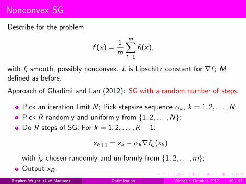
Nonconvex SG

Describe for the problem

f (x) =1

m

m∑i=1

fi (x),

with fi smooth, possibly nonconvex. L is Lipschitz constant for ∇f ; Mdefined as before.

Approach of Ghadimi and Lan (2012): SG with a random number of steps.

Pick an iteration limit N; Pick stepsize sequence αk , k = 1, 2, . . . ,N;

Pick R randomly and uniformly from 1, 2, . . . ,N;Do R steps of SG: For k = 1, 2, . . . ,R − 1:

xk+1 = xk − αk∇fik (xk)

with ik chosen randomly and uniformly from 1, 2, . . . ,m;Output xR .


Convergence for Nonconvex SG

Constant-step variant:

αk ≡ min

1

L,

D

M√N

,

for some user-defined D > 0.

Define Df so that D2f = 2(f (x1)− f ∗)/L (where f ∗ is the optimal value of

f ). Then1

LE [‖∇f (xR)‖2] ≤

LD2f

N+

(D +

D2f

D

)M√N.

In the case of convex f , get a similar bound:

E [f (xR)− f ∗] ≤LD2

X

N+

(D +

D2X

D

)M√N,

where DX = ‖x1 − x∗‖.Stephen Wright (UW-Madison) Optimization Winedale, October, 2012 41 / 67

Two-Phase Nonconvex SG

Ghadimi and Lan extend this method to achieve complexity like 1/k, byrunning multiple processes in parallel, and picking the solution with thebest sample gradient. Prove a large-deviation convergence bound: userspecifies required threshold ε for ‖∇f (x)‖2, and required likelihood 1− Λ(for small positive Λ).

Choose trial set j1, j2, . . . , jT of indices from 1, 2, . . . ,m.Set S = log(2/Λ);

For s = 1, 2, . . . ,S , run SG with random number of iterates, toproduce xs ;

For s = 1, 2, . . . ,S , calculate

gs =1

T

T∑k=1

∇fjk (xs).

Output xs for which ‖gs‖ is minimized.


Sparse Optimization: Motivation

Many applications need structured, approximate solutions of optimizationformulations, rather than exact solutions.

More Useful, More Credible

Structured solutions are easier to understand.They correspond better to prior knowledge about the solution.They may be easier to use and actuate.Extract just the essential meaning from the data set, not the lessimportant effects.

Less Data Needed

Structured solution lies in lower-dimensional spaces ⇒ need to gather /sample less data to capture it.

The structural requirements have deep implications for how we formulateand solve these problems.


Regularized Formulations: Shrinking Algorithms

Consider the formulation

minx

f (x) + τψ(x).

Regularizer ψ is often nonsmooth but “simple.” Often the problem is easyto solve when f is replaced by a quadratic with diagonal Hessian:

minz

gT (z − x) +1

2α‖z − x‖2

2 + τψ(z).

Equivalently,

minz

1

2α‖z − (x − αg)‖2

2 + τψ(z).

Define the shrink operator as the arg min:

Sτ (y , α) := arg minz

1

2α‖z − y‖2

2 + τψ(z).


Interesting Regularizers and their Shrinks

Cases for which the subproblem is simple:

ψ(z) = ‖z‖1. Thus Sτ (y , α) = sign(y) max(|y | − ατ, 0). When ycomplex, have

Sτ (y , α) =max(|y | − τα, 0)

max(|y | − τα, 0) + ταy .

ψ(z) =∑

g∈G ‖z[g ]‖2, where z[g ], g ∈ G are non-overlappingsubvectors of z . Here

Sτ (y , α)[g ] =max(|y[g ]| − τα, 0)

max(|y[g ]| − τα, 0) + ταy[g ].

ψ(x) = IΩ(x): Indicator function for a closed convex set Ω. ThenSτ (y , α) is the projection of y onto Ω.


Basic Prox-Linear Algorithm

(Fukushima and Mine, 1981) for solving minx f (x) + τψ(x).

0: Choose x0

k : Choose αk > 0 and set

xk+1 = Sτ (xk − αk∇f (xk);αk)

= arg minz∇f (xk)T (z − xk) +

1

2αk‖z − xk‖2

2 + τψ(z).

This approach goes by many names, including forward-backward splitting,shrinking / thresholding.

Straightforward, but can be fast when the regularization is strong (i.e.solution is “highly constrained”).

Can show convergence for steps αk ∈ (0, 2/L), where L is the bound on∇2f . (Like a short-step gradient method.)


Enhancements

Alternatively, since αk plays the role of a steplength, can adjust it to getbetter performance and guaranteed convergence.

Backtracking: decrease αk until sufficient decrease condition holds.

Use Barzilai-Borwein strategies to get nonmonotonic methods. Byenforcing sufficient decrease every 10 iterations (say), still get globalconvergence.

Embed accelerated first-order methods (e.g. FISTA) by redefining thelinear term g appropriately.

Do continuation on the parameter τ . Solve first for large τ (easierproblem) then decrease τ in steps toward a target, using the previoussolution as a warm start for the next value.


Decomposition / Coordinate Relaxation

For min f (x), at iteration k, choose a subset Gk ⊂ 1, 2, . . . , n and takea step dk only in these components. i.e. fix [dk ]i = 0 for i /∈ Gk .

Fewer variables ⇒ smaller and cheaper to deal with than the full problem.Can

take a reduced gradient step in the Gk components;

take multiple “inner iterations”

actually solve the reduced subproblem in the space defined by Gk .


Example: Decomposition in SVM

Decomposition has long been popular for solving the dual (QP)formulation of support vector machines (SVM), since the number ofvariables (= number of training examples) may be very large.

SMO, LIBSVM: Each Gk has two components, different heuristicsfor choosing Gk .

LASVM: Again |Gk | = 2, with focus on online setting.

SVM-light: Small |Gk | (default 10).

GPDT: Larger |Gk | (default 400) with gradient projection solver asinner loop.


Deterministic Results

Generalized Gauss-Seidel condition requires only that each coordinate is“touched” at least once every T iterations:

Gk ∪ Gk+1 ∪ . . . ∪ Gk+T−1 = 1, 2, . . . , n.

Can show global convergence (e.g. Tseng and Yun, 2009; Wright, 2012).

There are also results on

global linear convergence rates;

optimal manifold identification (for problems with nonsmoothregularizer);

fast local convergence for an algorithm that takes reduced steps onthe estimated optimal manifold.


Stochastic Coordinate Descent

Randomized coordinate descent (RCDC)

(Richtarik and Takac, 2012; see also Nesterov, 2012)

For min f (x).

Partitions the components of x into subvectors;

Makes a random selection of one partition to update at each iteration;

Exploits knowledge of the partial Lipschitz constant for each partitionin choosing the step.

Allows parallel implementation.

At each iteration, pick a partition at random, and take a short-stepsteepest descent step on the variables in that component.


RCDC Details

Partition components 1, 2, . . . , n into m blocks with block [i ] withcorresponding columns from the n × n identity matrix denoted by Ui .

Denote by Li the partial Lipschitz constant on partition [i ]:

‖∇[i ]f (x + Ui t)−∇[i ]f (x)‖ ≤ Li‖t‖.

Fix probabilities of choosing each partition: pi , i = 1, 2, . . . ,m.

Iteration k :

Choose partition ik ∈ 1, 2, . . . ,m with probability pi ;

Set dk,i = −(1/Lik )∇[ik ]f (xk);

Set xk+1 = xk + Uikdk,i .

For convex f and uniform weights pi = 1/m, can prove high probabilityconvergence of f to within a specified threshold of f (x∗) in O(1/k)iterations.


RCDC Result

‖x‖L :=

(m∑i=1

Li‖x[i ]‖2

)1/2

Weighted measure of level set size:

RL(x) := maxy

maxx∗∈X∗

‖y − x∗‖L : f (y) ≤ f (x).

Assuming that desired precision ε has

ε < min(R2L(x0), f (x0)− f ∗)

and defining

K :=2nR2

L(x0)

εlog

f (x0)− f ∗

ερ,

we have for k ≥ K that

P(f (xk)− f ∗ ≤ ε) ≥ 1− ρ.


Augmented Lagrangian Methods and Splitting

Consider linearly constrained problem:

min f (x) s.t. Ax = b.

Augmented Lagrangian is

L(x , λ; ρ) := f (x) + λT (Ax − b) +ρ

2‖Ax − b‖2

2,

where ρ > 0. Basic augmented Lagrangian / method of multipliers is

xk = arg minxL(x , λk−1; ρk);

λk = λk−1 + ρk(Axk − b);

(choose ρk+1).

Extends to inequality constraints, nonlinear constraints.


Features of Augmented Lagrangian

If we set λ = 0, recover the quadratic penalty method.

If λ = λ∗, the minimizer of L(x , λ∗; ρ) is the true solution x∗, for anyρ ≥ 0.

AL provides successive estimates λk of λ∗, thus can achieve solutionswith good accuracy without driving ρk to ∞.


History of Augmented Lagrangian

Dates from 1969: Hestenes, Powell.

Developments in 1970s, early 1980s by Rockafellar, Bertsekas,....

Lancelot code for nonlinear programming: Conn, Gould, Toint,around 1990.

Largely lost favor as an approach for general nonlinear programmingduring the next 15 years.

Recent revival in the context of sparse optimization and associateddomain areas, in conjunction with splitting / coordinate descenttechniques.


Separable Objectives: ADMM

Alternating Directions Method of Multipliers (ADMM) arises when theobjective in the basic linearly constrained problem is separable:

min(x ,z)

f (x) + h(z) subject to Ax + Bz = c ,

for which

L(x , z , λ; ρ) := f (x) + h(z) + λT (Ax + Bz − c) +ρ

2‖Ax − Bz − c‖2

2.

Standard augmented Lagrangian would minimize L(x , z , λ; ρ) over (x , z)jointly — but these are coupled through the quadratic term, so theadvantage of separability is lost.

Instead, minimize over x and z separately and sequentially:

xk = arg minxL(x , zk−1, λk−1; ρk);

zk = arg minzL(xk , z , λk−1; ρk);

λk = λk−1 + ρk(Axk + Bzk − c).


ADMM

Each iteration does a round of block-coordinate descent in (x , z).

The minimizations over x and z add only a quadratic term to f andh, respectively. This does not alter the cost much.

Can perform these minimizations inexactly.

Convergence is often slow, but sufficient for many applications.

Many recent applications to compressed sensing, image processing,matrix completion, sparse PCA.

ADMM has a rich collection of antecendents. For an excellent recentsurvey, including a diverse collection of machine learning applications, see(Boyd et al, 2011).


ADMM for Consensus Optimization

Given

minm∑i=1

fi (x),

form m copies of the x , with the original x as a “master” variable:

minx ,x1,x2,...,xm

m∑i=1

fi (xi ) subject to x i = x , i = 1, 2, . . . ,m.

Apply ADMM, with z = (x1, x2, . . . , xm), get

x ik = arg minx i

fi (xi ) + (λik−1)T (x i − xk−1) +

ρk2‖x i − xk−1‖2

2, ∀i ,

xk =1

m

m∑i=1

(x ik +

1

ρkλik−1

),

λik = λik−1 + ρk(x ik − xk), ∀i

Can do the x i updates in parallel. Synchronize for x update.Stephen Wright (UW-Madison) Optimization Winedale, October, 2012 59 / 67

ADMM for Awkward Intersections

The feasible set is sometimes an intersection of two or more convex setsthat are easy to handle separately (e.g. projections are easily computable),but whose intersection is more difficult to work with.

Example: Optimization over the cone of doubly nonnegative matrices:

minX

f (X ) s.t. X 0, X ≥ 0.

General form:

min f (x) s.t. x ∈ Ωi , i = 1, 2, . . . ,m

Just consensus optimization, with indicator functions for the sets.

xk = arg minx

f (x) +m∑i=1

(λik−1)T (x − x ik−1) +ρk2‖x − x ik−1‖2

2,

x ik = arg minxi∈Ωi

(λik−1)T (xk − x i ) +ρk2‖xk − x i‖2

2, ∀i

λik = λik−1 + ρk(xk − x ik), ∀i .


Splitting+Lagrangian+Hogwild!

Recalling Hogwild! for minimizing

f (x) =m∑i=1

fi (x),

using parallel SG, where each core evaluates a random partial gradient∇fi (x) and updates a centrally stored x . Results were given showing goodspeedups on a 12-core machine.

The machine has two sockets, so need frequent cross-socket cache fetches.

Re et al (2012) use the same 12-core, 2-socket platform, but

each socket has its own copy of x , each updated by half the cores;

The copies “synchronize” periodically by consensus, or by updating acommon multiplier λ.


Details

Replace min f (x) by the split problem

minx ,z

f (z) + f (z) s.t. x = z .

Min-max formulation is

minx ,z

maxλ

f (x) + f (z) + λT (x − z).

Store x on one socket and z on the other. Algorithm step k:

Apply Hogwild independently on the two sockets, for a certainamount of time, to

minx

f (x) + λTk x , minz

f (z)− λTk z ,

To obtain xk and zk .

Swap values xk and zk between sockets and update

λk+1 := λk + γ(xk − zk), for some γ > 0.


Over 100 epochs for the SVM problem RCV1, without permutation,speedup factor is 4.6 (.77s vs .17s).


Partially Separable: Higher-Order Methods

Consider again

f (x) =1

m

m∑i=1

fi (x)

Newton’s method obtains step by solving

∇2f (xk)dk = −∇f (xk),

and setting xk+1 = xk + dk . We have

∇2f (x) =1

m

m∑i=1

∇2fi (x), ∇f (x) =1

m

m∑i=1

∇fi (x).

The “obvious” implementation requires scan through the complete dataset, and formation and solution of an n × n linear system. This is usuallyimpractical for large m, n.


Sampling

(Martens, 2010; Byrd et al, 2011)

Approximate the derivatives by sampling over a subset of the m terms.

Choose X ⊂ 1, 2, . . . ,m and S ⊂ X , and set

HkS =

1

|S |∑i∈S∇2fi (xk), gk

X =1

|X |∑i∈X∇fi (xk).

Approximate Newton step satisfies

HkSdk = gk

X .

Typically, S is just 1% to 10% of the terms.


Conjugate Gradient and “Hessian-Free” Implementation

We can use conjugate gradient (CG) to find an approximate solution.Each iteration of CG requires one matrix-vector multiplication with Hk

S ,plus some vector operations (O(n) cost).

Hessian-vector product

HkSv =

1

|S |∑i∈S∇2fi (xk)v .

Since ∇2fi often is sparse, each product ∇2fi (xk)v is cheap.

We can even avoid second-derivative calculations altogether, by usingfinite-difference approximation to the matrix-vector product:

∇2fi (xk)v ≈ [∇fi (xk + εv)−∇fi (xk)]/ε.

Sampling and coordinate descent can be combined: see Wright (2012) forapplication of this combination to regularized logistic regression.


Conclusions

I’ve given an incomplete survey of optimization techniques that may beuseful in analysis of large datasets, particularly for learning problems.

Some important topics omitted, e.g.

quasi-Newton methods (L-BFGS),

nonconvex regularizers,

manifold identification / variable selection.

For further information, see slides, videos, and reading lists for tutorialsthat I have presented recently, on some of these topics. Or mail me.

FIN


Documents

Optimization Algorithms for Analyzing Large Datasets