Optimization and Control Design of an Autonomous

Underwater Vehicle

A Major Qualifying Project Report:

Submitted to the Faculty of the

WORCESTER POLYTECHNIC INSTITUTE

in partial fulfillment of the requirements for

the Degree of Bachelor of Science

in Aerospace Engineering

By

Umut Tekin ____________________________

Date: 01/10/2011

Approved by _____________________________

Professor Islam Hussein, Major Advisor

Keywords 1. Autonomous

2. Submarine

3. Hydrodynamic

Certain materials are included under the fair use exemption of the U.S. Copyright Law and have been prepared according to the fair use guidelines and are restricted from further use.

Abstract

Autonomous vehicles are increasingly being investigated for use in oceanographic studies,

underwater surveillance, and search operations. Research currently being done in the area

of autonomous underwater craft is often hindered by expense. This project seeks to

complete the construction, optimization, control software development of an inexpensive

miniature underwater vehicle. During the course of the project all of the vehicle’s

mechanical, electrical subsystems and control algorithms were completed.

Propeller-driven primary thrusters using a magnetically coupled drive system were

optimized and manufactured. A battery powered electrical subsystem was also designed

and installed on the vehicle. A simulation of the vehicle’s control algorithm was developed

in MATLAB.

Executive Summary

The primary purpose for the 20010-2011 Autonomous Underwater Vehicle (AUV) Major

Qualifying Project (MQP) was to program, optimize, and complete work on an existing

submersible platform built by the AUV MQP group from the 2008-2009 school year. Upon

completion, this vehicle will provide a low cost, highly adaptable platform for testing

autonomous software and hardware. The are AUV platforms that are available in the

market for the commercial uses are typically too expensive or not adaptable enough to test

various systems.

In order to complete the objective the group have fabricated and optimized various

hardware and integrated vehicle simulations into vehicle programs along with the control

algorithms.

Acknowledgements

We would like to thank Professor Islam Hussein and Professor William Michalson for

their guidance and expertise throughout the duration of this project.

Nomenclature

E, V Volts

I Amperes

W Watts

m Meters

m/s Meters per Second

s Seconds

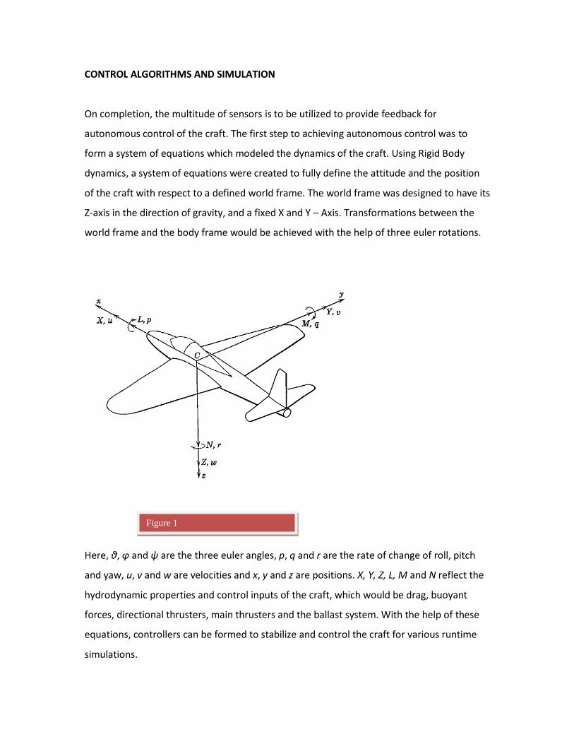
CONTROL ALGORITHMS AND SIMULATION

On completion, the multitude of sensors is to be utilized to provide feedback for

autonomous control of the craft. The first step to achieving autonomous control was to

form a system of equations which modeled the dynamics of the craft. Using Rigid Body

dynamics, a system of equations were created to fully define the attitude and the position

of the craft with respect to a defined world frame. The world frame was designed to have its

Z-axis in the direction of gravity, and a fixed X and Y – Axis. Transformations between the

world frame and the body frame would be achieved with the help of three euler rotations.

Here, θ, φ and ψ are the three euler angles, p, q and r are the rate of change of roll, pitch

and yaw, u, v and w are velocities and x, y and z are positions. X, Y, Z, L, M and N reflect the

hydrodynamic properties and control inputs of the craft, which would be drag, buoyant

forces, directional thrusters, main thrusters and the ballast system. With the help of these

equations, controllers can be formed to stabilize and control the craft for various runtime

simulations.

Figure 1

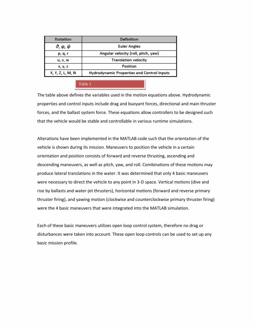
The table above defines the variables used in the motion equations above. Hydrodynamic

properties and control inputs include drag and buoyant forces, directional and main thruster

forces, and the ballast system force. These equations allow controllers to be designed such

that the vehicle would be stable and controllable in various runtime simulations.

Alterations have been implemented in the MATLAB code such that the orientation of the

vehicle is shown during its mission. Maneuvers to position the vehicle in a certain

orientation and position consists of forward and reverse thrusting, ascending and

descending maneuvers, as well as pitch, yaw, and roll. Combinations of these motions may

produce lateral translations in the water. It was determined that only 4 basic maneuvers

were necessary to direct the vehicle to any point in 3-D space. Vertical motions (dive and

rise by ballasts and water-jet thrusters), horizontal motions (forward and reverse primary

thruster firing), and yawing motion (clockwise and counterclockwise primary thruster firing)

were the 4 basic maneuvers that were integrated into the MATLAB simulation.

Each of these basic maneuvers utilizes open loop control system, therefore no drag or

disturbances were taken into account. These open loop controls can be used to set up any

basic mission profile.

Table 1

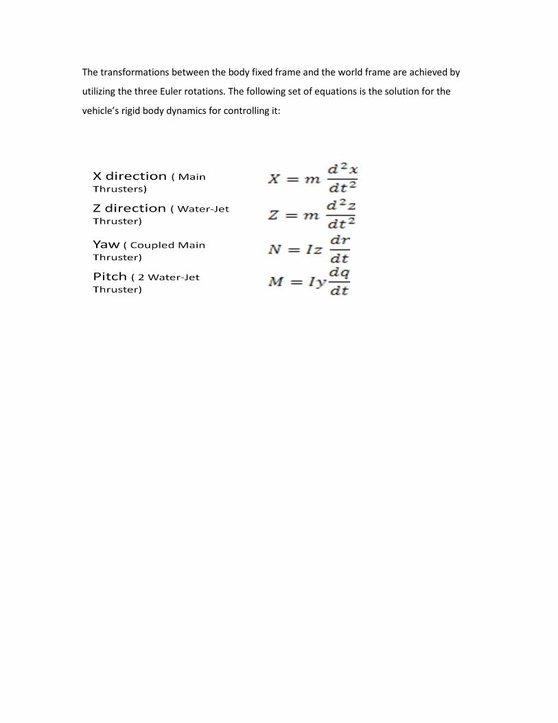
The transformations between the body fixed frame and the world frame are achieved by

utilizing the three Euler rotations. The following set of equations is the solution for the

vehicle’s rigid body dynamics for controlling it:

Horizontal Maneuver

In the MATLAB simulation, the horizontal axis motions are determined only using

time-based commands. Using given user inputs of the initial and final vehicle positions, a

total trip time is determined. This value is halved to split the maneuver into two stages.

Since no disturbances are accounted for, the only control forces implemented are the ones

from the primary thrusters. First, the program will determine whether a forward or reverse

maneuver is required; this is accomplished with the utilization of the initial and final

positions, accounting for accelerating and decelerating the vehicle.

Yaw Maneuver

Similar to the horizontal maneuver, the yawing motion implements a similar control

algorithm. Time is initially determined and then halved to split the maneuver into separate

parts, accounting for accelerating and decelerating the vehicle. The force of each thruster is

multiplied by the distance to the vehicle center, resulting in a produced torque. The total

torque of the system is calculated by summing the torque produced by each of the

thrusters. This, in combination with the moment of inertia in the Z direction, provides the

angular acceleration of the craft. Using the simple rotational motion physics equation, a

total trip time is derived by the program. The initial angular velocity is assumed to be zero.

Once the time is computed, the first leg of the mission will provide a moment accelerating

the vehicle in a CW or CCW direction, depending on the initial and final conditions. To stop

the vehicle’s angular acceleration, an opposite moment is applied causing the vehicle to

brake and stop at the final destination.

Pitch Maneuver

Finally the pitch maneuver simulated is similar to the vertical Z-axis thrust maneuver except

this motions is to use either both front or both rear jet-thrusters at a time to make possible

for a pitch effect on the forces of the vehicle of the longer axis and while the ballast tanks

are stabilized in their former state of pressure. But if the vehicle was to be simulated for the

shorter axis pitch, then either right or the left side jets would be used to accomplish the

desired similar effect.

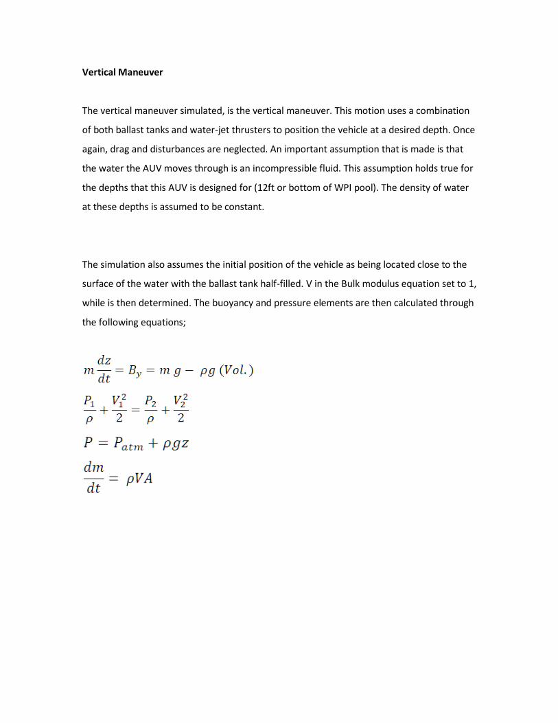
Vertical Maneuver

The vertical maneuver simulated, is the vertical maneuver. This motion uses a combination

of both ballast tanks and water-jet thrusters to position the vehicle at a desired depth. Once

again, drag and disturbances are neglected. An important assumption that is made is that

the water the AUV moves through is an incompressible fluid. This assumption holds true for

the depths that this AUV is designed for (12ft or bottom of WPI pool). The density of water

at these depths is assumed to be constant.

The simulation also assumes the initial position of the vehicle as being located close to the

surface of the water with the ballast tank half-filled. V in the Bulk modulus equation set to 1,

while is then determined. The buoyancy and pressure elements are then calculated through

the following equations;

MATLAB RESULTS

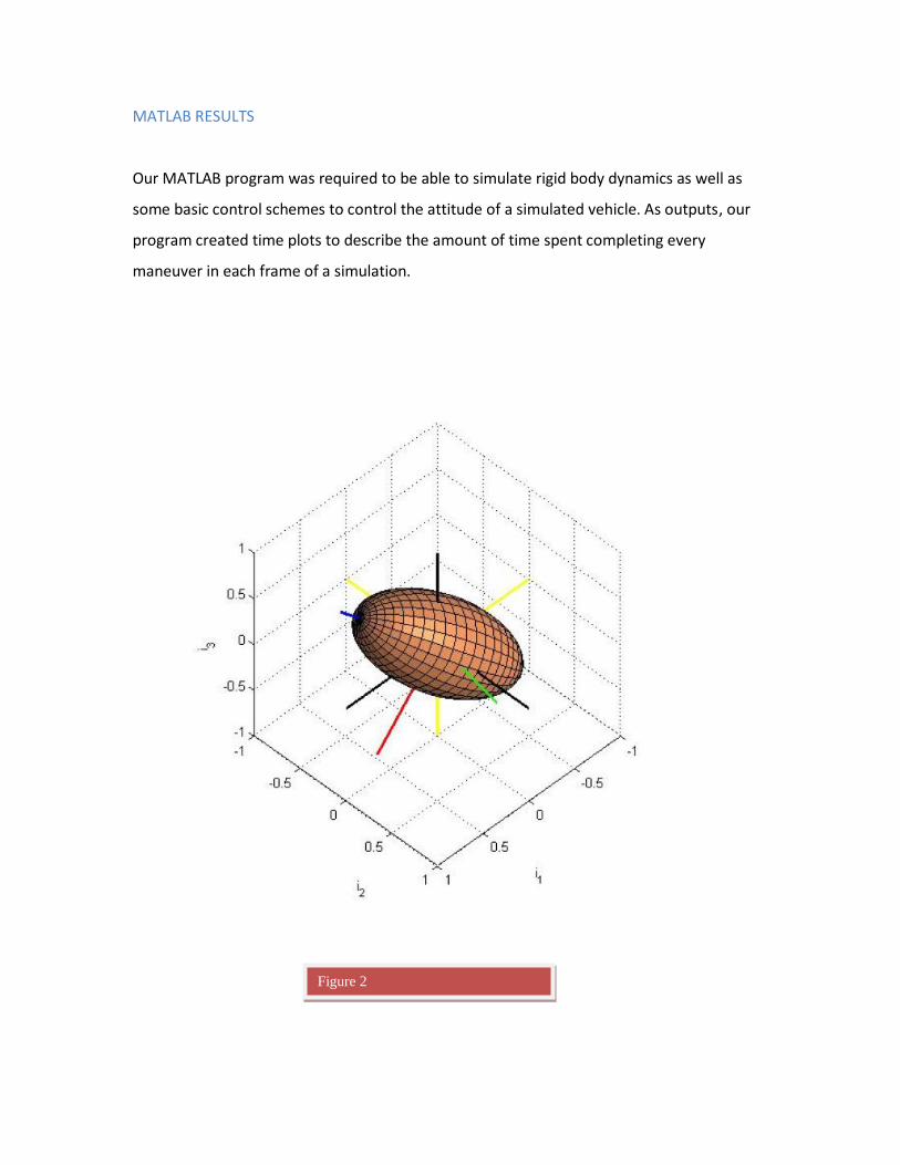
Our MATLAB program was required to be able to simulate rigid body dynamics as well as

some basic control schemes to control the attitude of a simulated vehicle. As outputs, our

program created time plots to describe the amount of time spent completing every

maneuver in each frame of a simulation.

Figure 2

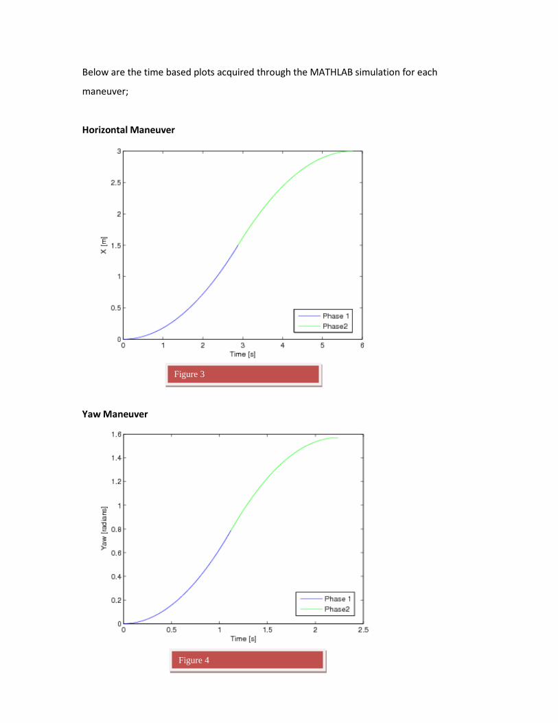
Below are the time based plots acquired through the MATHLAB simulation for each

maneuver;

Horizontal Maneuver

Yaw Maneuver

Figure 3

Figure 4

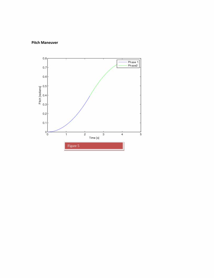
Pitch Maneuver

Figure 5

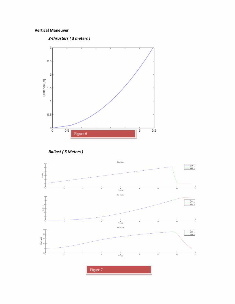
Vertical Maneuver

Z-thrusters ( 3 meters )

Ballast ( 5 Meters )

Figure 6

Figure 7

Alterations have been implemented in the MATLAB code such that the orientation of the

vehicle is shown during its mission. Maneuvers to position the vehicle in a certain

orientation and position consists of forward and reverse thrusting, ascending and

descending maneuvers, as well as pitch, yaw, and roll. Combinations of these motions may

produce lateral translations in the water. It was determined that 4 basic maneuvers were

necessary to direct the vehicle to any point in 3-D space. Vertical motions (dive and rise by

ballasts and water-jet thrusters), horizontal motions (forward and reverse primary thruster

firing), and yawing motion (clockwise and counterclockwise primary thruster firing) were

the 4 basic maneuvers that were integrated into the MATLAB simulation.

Each of these basic maneuvers utilized in an open loop control system, therefore no drag or

disturbances were taken into account. These open loop controls can be used to set up any

basic mission profile. These files can be found in: MATLAB Code. The simulation of

horizontal control requires the user to input the initial and final positions of the vehicle.

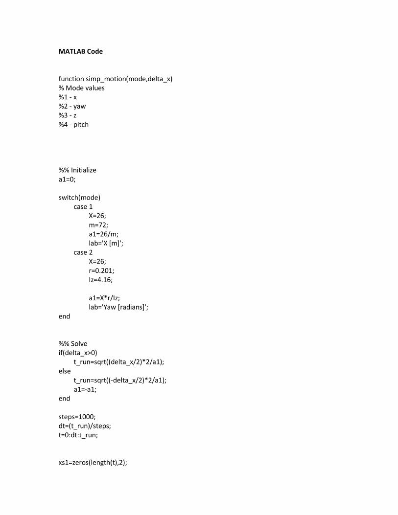
MATLAB Code

function simp_motion(mode,delta_x) % Mode values %1 - x %2 - yaw %3 - z %4 - pitch %% Initialize a1=0; switch(mode) case 1 X=26; m=72; a1=26/m; lab='X [m]'; case 2 X=26; r=0.201; Iz=4.16; a1=X*r/Iz; lab='Yaw [radians]'; end %% Solve if(delta_x>0) t_run=sqrt((delta_x/2)*2/a1); else t_run=sqrt((-delta_x/2)*2/a1); a1=-a1; end steps=1000; dt=(t_run)/steps; t=0:dt:t_run; xs1=zeros(length(t),2);

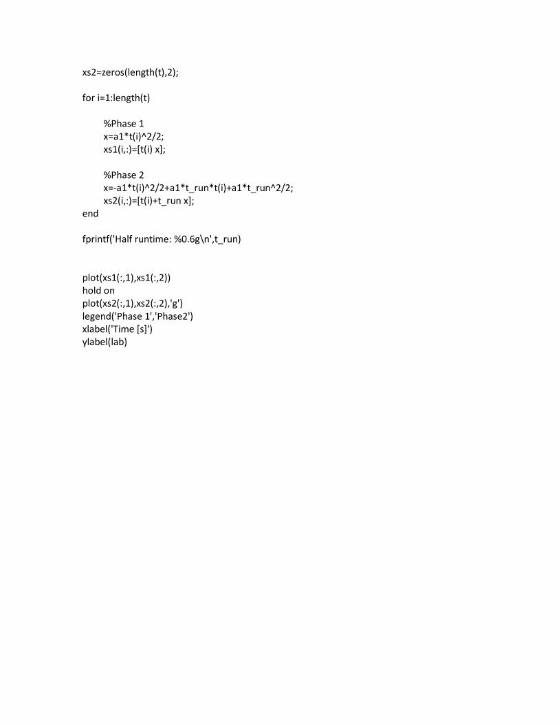
xs2=zeros(length(t),2); for i=1:length(t) %Phase 1 x=a1*t(i)^2/2; xs1(i,:)=[t(i) x]; %Phase 2 x=-a1*t(i)^2/2+a1*t_run*t(i)+a1*t_run^2/2; xs2(i,:)=[t(i)+t_run x]; end fprintf('Half runtime: %0.6g\n',t_run) plot(xs1(:,1),xs1(:,2)) hold on plot(xs2(:,1),xs2(:,2),'g') legend('Phase 1','Phase2') xlabel('Time [s]') ylabel(lab)

REFERENCES

___________________________________________________________________

[1] Louis V. Schmidt; AIAA 1998; “Introduction to aircraft flight dynamics”

[2] Etkin, Bernard; New York, Wiley [1972]; “Dynamics of atmospheric flight”