University of MississippieGrove

Honors Theses Honors College (Sally McDonnell BarksdaleHonors College)

2019

Optimization and Cost Comparison of ReactorTypes in a Styrene Production ProcessClaire Lenore CozaddUniversity of Mississippi

Follow this and additional works at: https://egrove.olemiss.edu/hon_thesisPart of the Chemical Engineering Commons

This Undergraduate Thesis is brought to you for free and open access by the Honors College (Sally McDonnell Barksdale Honors College) at eGrove. Ithas been accepted for inclusion in Honors Theses by an authorized administrator of eGrove. For more information, please contact egrove@olemiss.edu.

Recommended CitationCozadd, Claire Lenore, "Optimization and Cost Comparison of Reactor Types in a Styrene Production Process" (2019). HonorsTheses. 1067.https://egrove.olemiss.edu/hon_thesis/1067

OPTIMIZATION AND COST COMPARISON OF REACTOR TYPES

IN A STYRENE PRODUCTION PROCESS

by

Claire Lenore Cozadd

A thesis submitted to the faculty of The University of Mississippi in partial fulfillment of

the requirements of the Sally McDonnell Barksdale Honors College.

Oxford

May 2019

Approved by

_______________________________

Advisor: Dr. Adam Smith

_______________________________

Reader: Dr. Alexander Lopez

_______________________________

Reader: Dr. Wei-Yin Chen

ii

Dedication

To Gordon and Jo Cozadd, my Gampy and Diggy,

for instilling in me a love of learning from a very young age

and for being my best friends.

iii

Acknowledgements

There are several people without whom this thesis would not have been possible.

First, I want to thank Dr. Adam Smith, who was willing to become my thesis adviser

even when I asked him at the very end of last semester. He provided me with excellent

teaching in ChE 308 and 451 as well as guidance throughout this entire project, and I

sincerely appreciate it.

I also want to thank all of the other members of the Ole Miss Chemical Engineering

faculty with whom I have taken classes. This includes Dr. John O’Haver, Dr. Sasan

Nouranian, Dr. Esteban Ureña-Benavides, Dr. Brenda Prager, Dr. Alexander Lopez,

David Carrol, Dr. Alireza Asiaee, and Mike Gill. Each of them has shared their expertise

in all aspects of Chemical Engineering (and always made themselves available to answer

any silly question I may have), and they make our department top-notch.

In addition, I want to thank Mitch Sypniewski, Seth Gray, and Arizona Morgan-Harris

for working with me this entire school year to complete this project. Without their hard

work and willingness to put in long hours of work, this project would not have been

completed.

I lastly want to thank my family and all my friends. Each of them helped to make my

time at Ole Miss a positive one, and I will never forget it.

iv

Abstract

The focus of this thesis is to use the equivalent annual operating costs of isothermal,

adiabatic, and packed bed reactors in order to determine which reactor is most cost

effective in a styrene production process. In order to understand the steps leading up to

this comparison, background information is first given regarding chemical engineering

design, optimization, and process simulation. This information was necessary for

completing the ChE 451 design project, which was to analyze the base case styrene

process before optimizing it, in fall 2018. The results of this project are briefly outlined in

the second section. The third section discusses fluidized bed reactors and the process

which must be taken to model it in Excel. In this project, the selected configuration is

three fluidized bed reactors, each with a volume of approximately 83 m3, in parallel. The

last section discusses the calculation of equivalent annual operating costs for the

isothermal, adiabatic, and fluidized bed reactors. Overall, fluidized bed reactors are found

to be the most cost effective in the styrene process based on the equivalent annual

operating costs; however, a comparison based on the net present value of the entire

styrene process containing each reactor would yield a more accurate comparison.

v

TABLE OF CONTENTS

CHAPTER 1: INTRODUCTION 1

I. Introduction to Chemical Engineering Design 1

II. Introduction to Optimization 2

III. Introduction to Process Simulation 7

CHAPTER 2: THE DESIGN PROJECT 10

I. Base Case and Project Description 10

II. Continuing Work 12

CHAPTER 3: THE FLUIDIZED BED REACTOR 13

I. Introduction to the Fluidized Bed Reactor 13

II. Given Values and Assumptions for a Fluidized Bed Reactor 14

III. Algorithm for Fluidized Bed Reactor Calculations in Excel 16

IV. The Selection of the Fluidized Bed Reactor Configuration 19

CHAPTER 4: COMPARING REACTORS BASED ON EAOCs 20

CHAPTER 5: CONCLUSION 24

APPENDICES 25

I. Appendix A- Styrene Process Optimization Design Report (written with

Seth Gray and Mitch Sypniewski in ChE 451, Fall 2018) 26

II. Appendix B- Base and Optimized Case Specifications 36

III. Appendix C- Optimization Materials and Steps 51

IV. Appendix D- Miscellaneous Information 55

V. Appendix E- Fluidized Bed Reactor Pro-II Simulation 59

REFERENCES 61

1

Chapter 1: Introduction

I. Introduction to Chemical Engineering Design

In their careers both as students and as professionals in industry, chemical

engineers will likely be required to complete process design. Process design starts with

defining a customer need and then developing profitable solutions to fulfill it. For

chemical engineers, design projects focus on chemical processes and plants. In industry,

one can expect to encounter three types of projects: modification to existing plants,

scaling to a new production capacity, and design of a new process. The first makes up

50% of all projects, the second 45%, and the last only 5%.

Ultimately, the design process can be seen as the culmination of the entire

chemical engineering field. It requires the engineer to demonstrate an understanding of

mass and energy balances, separations and reactor unit principles, equipment sizing

heuristics, and economic terms and calculations. However, the engineer must also take

into account the constraints on the process due to the physical properties of its

components, the local, state, and federal government regulations, the properties of the

equipment materials, and the economics. To determine the best design for a specific

process, the design process will be completed iteratively.

The design process has seven steps that fit into two phases: process design and

plant design. Process design begins with identifying the design objective. The design

basis is then set, and this takes into account the desired production rate and purity, the

system of units, the design codes, the raw materials, and the utilities. Next, potential

design concepts are generated, and these undergo analysis and evaluation in computer

2

simulations before one is ultimately selected. Plant design begins with creating a detailed

equipment design. Then, it undergoes procurement and construction before it begins

operation.

II. Introduction to Optimization

Although designing a new process is the least encountered project in the

workplace, it remains important for the chemical engineer to know how to navigate the

design process for a new plant. In addition to testing the engineer’s overall knowledge of

the field, it tests whether one really understands how to utilize optimization. This plays a

key role in the analysis and evaluation of the potential design concepts for a process, and

it can determine whether the overall project will even be fit for implementation.

According to Richard Turton’s “Analysis, Synthesis, and Design of Chemical

Processes,” optimization “is the process of improving an existing situation, device, or

system such as a chemical process.” The goal of optimization is to find the best possible

setup for the chemical process. Engineers work toward this best setup by changing

specifications from a preliminary process design called a base case. Certain aspects of the

process, such as its primary product and the sections of the plant, will not change during

the optimization process. Therefore, an engineer must analyze the process to find

potential improvements in operating conditions. These are called design variables, and

they can be categorized as either continuous or discrete. Continuous variables, such as the

temperatures and pressures in towers and reactors, can take any value within specified

boundaries, or constraints. Discrete variables, such as the number of trays in a tower,

must have integer values.

3

In order to quantify the degree of improvement resulting from a change in the

process, there must be a defined point of comparison directly affected by the values of the

decision variables. In the optimization process, this is called the objective function. If the

objective function is a cost, it must be minimized during optimization; likewise, if it is a

profit, it must be maximized. Ultimately, there are two different types of optimums that

can result during optimization. The first is a global optimum, which results from

completing continuous optimization and represents the best possible case of all the

possible values of decision variables. This means that even making very small changes to

the decision variables would worsen the value of the objective function. While finding

this global optimum sounds ideal, it is near impossible for complex processes. It requires

an immense amount of effort and time to evaluate so many minute changes to each

decision variable. In addition, an actual process behaves differently than a computer

model; therefore, the best case defined on paper may be different than what is best for

actual operation.

Engineers want to avoid being bogged down in minute details associated with

finding a global optimum. As a result, they will instead utilize discrete optimization. This

means that, for any decision variable, the engineer will reanalyze the stream flowsheet

and economic model for only a few specific points. The rule for selecting these points is

simple: for each variable relating to equipment size, choose values that exist in the real

world. While the actual optimum reactor size may be 46.857 cubic meters, it is difficult

to get a reactor volume that accurate; therefore, whole number values should be tested

instead. Based on the behavior of the objective function as these points change, the

engineer will select the optimum. Depending on the project’s time constraints, the

4

engineer may refine this optimum to get closer to the global optimum’s value; however,

that is not necessary as long as justification is given for the engineer’s choice. This

method ultimately makes the optimization and design processes much more creative, as

there could be any number of scenarios that could be considered the best. It all depends

on the engineering team’s approach to the problem, because the order of the optimization

steps as well as the selected process changes made can vary greatly.

There are two types of optimization that an engineer will utilize on the process

design: topological and parametric. Topological deals with the type of equipment present

as well as how it is arranged within the plant, and it should be considered first.

Ultimately, the engineer must keep four main considerations in mind when utilizing this

type of optimization. One is to determine whether unwanted nonhazardous by-products

(which cannot be sold for profit) or hazardous waste streams (which must be treated) can

be eliminated. To do this, the engineer must maximize the conversion of the reactants as

well as the selectivity to the desired product. In some cases, the selectivity to the desired

product may decrease as the reactant conversion increases; therefore, in that case the

engineer will likely prefer the high selectivity as that reduces the number of by-product

streams more effectively. Another consideration is to determine if any equipment can be

eliminated or rearranged. Engineers typically examine possible equipment eliminations

after changing operating conditions, as this can cause some equipment from the original

PFD to be redundant. Equipment rearrangements, on the other hand, are typically

employed in the separation section of the process to avoid compressing gases and instead

pump liquids. The third is to consider the reactor and separations sections and determine

if alternative methods or configurations would work. For example, distillation is the most

5

common method used to separate liquids in industry because of its established technology

and low energy cost compared to other separators. However, alternative methods may

require implementation if the relative volatilities of the components needing to be

separated are close to 1 or if the mixture requires high pressure or low temperature

conditions for vapor-liquid equilibrium. The last is to consider heat integration and

determine how much it can be improved. Ultimately, this potentially reduces the annual

utilities cost by utilizing process streams as heating fluid.

Parametric optimization concerns operating variables, which can include

temperature, pressure, and concentrations of components in streams, for a piece of

equipment. The ones important to a specific system must be identified early in the

optimization process in order to reduce the time and effort the problem will require. This

also eliminates the possibility of investigating too many variables that will have little to

no effect on the objective function. For most processes, the engineer must consider

properties of the reactor, recycle, and separations sections. First, the engineer can

optimize the reactor’s operating conditions and single-pass conversion. The operating

conditions include pressure, reactant concentrations, and temperature, which is typically

constrained by the reaction’s catalyst properties. Ultimately, these variable changes affect

the reaction’s selectivity. For the recycle streams, the engineer can optimize the recovery

of unused reactants as well as the purge ratios if inert components, such as steam, are

utilized as dilutants. Lastly, for the separations section, variables typically depend upon

the separator type selected. In columns, the reflux ratio as well as the component

recoveries in the vapor and distillate streams can vary; however, in absorbers, strippers,

and extractors, the engineer can vary the amount of mass separating agent fed. Regardless

6

of separator type, though, the engineer should investigate changing the separator’s

operating pressure.

During the optimization process, engineers strategize the order in which to best

complete the topological and parametric optimizations. Ultimately, this results in them

either employing the top-down or bottom-up strategy. The top-down strategy consists of

the engineer beginning by analyzing the big picture (thus completing topological

optimization) before completing an analysis of the smaller details (thus completing

parametric optimization). For example, an engineer would start the optimization process

by examining the process flowsheet and asking if certain heat exchangers are actually

necessary. The bottom-up strategy is the opposite; therefore, the engineer starts by

investigating the smaller details of the process before looking at the process as a whole.

For example, the engineer might start the optimization process by investigating the effect

of changing the heating duties of the same heat exchangers. Regardless of whether the

engineer employs the top-down or bottom-up strategies, he or she will reach nearly the

same solution with these example starting points.

Experienced engineers, however, follow a slightly different strategy. Depending

on how the optimization is progressing, he may utilize either the top-down or bottom-up

strategy interchangeably. If the engineer is utilizing the bottom-up strategy and the

calculations concerning specific details of the process are taking too long, he will switch

back to the top-down strategy and check the broader design. Conversely, if the engineer

is utilizing the top-down strategy and the analysis of the whole process gives ambiguous

or indefinite results, he will switch back to the calculations for the specific process

7

details. Completing these switches efficiently requires the engineer to be flexible and

employ engineering intuition, which is gained through experience.

III. Introduction to Process Simulation

To assist with the rigorous calculations utilized in the design and operation of a

plant, a chemical engineer can utilize process simulations. These include computer

programs (such as CHEMCAD, Aspen Plus, HYSYS, PRO/II, or SuperPro Designer)

which can typically handle batch, semi-batch, and continuous processes with varying

success. Overall, the utilization of these products by chemical engineering students is

especially important in recent years. This is because companies are expecting entry-level

engineers to already have knowledge of the principles common to all the simulation

programs.

Ultimately, any simulation has seven input steps. The first two are preliminary

steps to creating the actual process flowsheet. Therefore, the user begins the simulation

by selecting the chemical components in the process from the program’s component

database. This is not limited only to the reactants and main products of the process;

therefore, inert compounds, by-products, utilities, and waste compounds must also be

included. If by chance a chemical in the process is not listed in the database, each

program should include directions for the user to add them. Next, the user selects the

thermodynamic model for the process. This is important for the simulator to be able to

adequately predict the phase equilibria of each component in the system. Therefore, this

gives the simulator access to each pure component’s heat capacity, density, and critical

constants. Also, in order to help the user to select the correct thermodynamic package,

some simulators have “expert systems”; however, these selections are typically based on

8

temperatures and pressures provided by the user, so they should not be viewed as

unalterable.

The next three steps involve inputting details for the process flowsheet. This

begins with selecting and inputting the process topology into the simulator. This

ultimately builds a virtual process flow diagram; however, it is most effective to plan the

process flow diagram on paper before attempting to construct it in the simulator. Also,

while most unit operations translate directly into the program, mixing points and splitting

points do not. Therefore, they require “phantom” unit operations simply called “mixers”

and “splitters” to represent them in a simulator. After the flowsheet is complete, the

process’s feed streams must be specified. For most streams, providing temperature and

pressure will be sufficient for this step. However, three feed conditions are an exception

because in these cases the feed stream’s temperature and pressure are not independent.

This includes saturated vapors, saturated liquids, and single component streams that have

two coexisting phases. The fifth is to input the process’s equipment specifications. These

allow the simulator to complete mass and energy balances on the process, and the

required parameters depend upon the equipment type. For example, pumps require only

one specification: either the outlet pressure or desired pressure increase. Rigorous

columns, on the other hand, require multiple specifications, including one for the number

of theoretical plates it contains, at least two to specify the behavior of the reboiler and the

condenser, and one for the feed tray.

The last two steps finalize the flowsheet and allow it to run properly. This begins

with the user deciding how the results will be displayed. Depending on what the user

wants to investigate, he or she can select to display the vapor and liquid component

9

flowrates in each stream or any number of charts detailing equipment performance,

including T-Q diagrams for heat exchangers and a composition profile for a trayed

column. Finally, the last step is to select convergence criteria and run the simulation [1].

The utilization of process simulation as well as the optimization process was key

to completing the following project.

10

Chapter 2: The Design Project

I. Base Case and Project Description

Landshark Inc. is considering implementing a styrene production process at its

OM petrochemical facility. The proposed process utilizes the dehydrogenation of

ethylbenzene to produce 100,000 tonnes of styrene per year with at least 99.5 weight

percent purity. Landshark Inc. will sell the styrene to manufacturers interested in

polymerizing it to make polystyrene packaging and foam insulation, which could

potentially be profitable.

Other constraints besides the styrene product purity for the Unit 500 process were

also indicated in the project description. These include component recoveries and unit

temperatures and pressures. First, the toluene recovery to the overhead stream and the

ethylbenzene recovery to the bottoms stream of tower T-501 must both be 99%. The

styrene recovery to the bottoms stream of tower T-502 must also be 99%. In addition, the

temperature in tower T-502 must be less than 125°C to avoid spontaneous polymerization

of the concentrated styrene. Also, the maximum temperature in the R-501 reactor scheme

is 1000 K, and the temperature drop across the reactor’s length must be less than 50 K.

The reactor’s pressure must also be between 0.75 and 2.5 bar.

Several assumptions were also required in order to set up the Excel model of the

styrene process. First, the streams behave as ideal gases and solutions; therefore, vapor-

liquid equilibrium calculations in this process must utilize Raoult’s Law. In addition,

perfect separation between the organic liquid and aqueous phases occurs in vessel V-501,

and any methane or hydrogen in the organic liquid is a dissolved gas. Finally, in the

11

tower section, the light key is the lightest component in the bottoms stream and the heavy

key is the heaviest component in the overhead stream.

Ultimately, the base case analysis was completed and the preliminary design’s

economic feasibility was determined. The plant originally had a NPV of -$320.3 M and

an AE of -$51.7 M with a MARR of 12%. This results in both a conventional and

discounted payback greater than 12 years. Because of the negative NPV and a payback

period longer than the project life, the project is not profitable using the preliminary

design.

However, several potential changes were noted that could improve the process

design. In the reactor section, the reactor type, temperatures, pressures and feed could be

changed. In the separation section, the vessel pressures as well as the tower inlet

temperatures and pressures could be adjusted. These all can be used as design variables.

In addition, an extra tower scheme could be added to purify the benzene stream and

increase the process revenue. Heat integration could also be implemented to possibly

reduce the process utility costs. Improvement will be quantified based on increase in

NPV, which is the objective function.

Ultimately, the changes made during the optimization process on the styrene plant

are detailed in the executive summary attached in Appendix A, but the most significant

changes are summarized here. First, the reactors (R-501 and R-502) were changed from

isothermal to adiabatic (therefore, their names changed to R-503 and R-504). In addition,

reactor R-503’s volume decreased from 50 to 36 m3 and its inlet temperature was reduced

from 550°C to 525°C. Also, the material of construction for the towers (T-501 and T-

502) was changed from titanium to carbon steel. Lastly, tower T-503 was added to

12

deliver a benzene product with a higher purity. Other minor improvements were made to

slightly improve the plant’s NPV or to ensure the plant could operate safely. Overall,

after completing the optimization process, the plant had an NPV of $31 M and a

discounted cash flow rate of return (DCFROR) of 16%. As a result, the plant was

profitable and could be recommended for further development.

II. Continuing Work

All work described previously primarily pertained to the styrene process design

project completed as required in the ChE 451 (the senior design course for chemical

engineers) curriculum. Therefore, to fulfill the capstone requirements for the Honors

College, previous work was expanded upon by investigating fluidized bed reactors as an

alternative to the isothermal and adiabatic reactors investigated previously.

13

Chapter 3: The Fluidized Bed Reactor

I. Introduction to the Fluidized Bed Reactor

Overall, a fluidized bed reactor is one which takes advantage of fluidization

theory. According to Cocco, Karri, and Knowlton of Particulate Solid Research, Inc.,

“particles become fluidized when an upward-flowing gas imposes a high enough drag

force [due to friction imposed by the gas on the particle] to overcome the downward

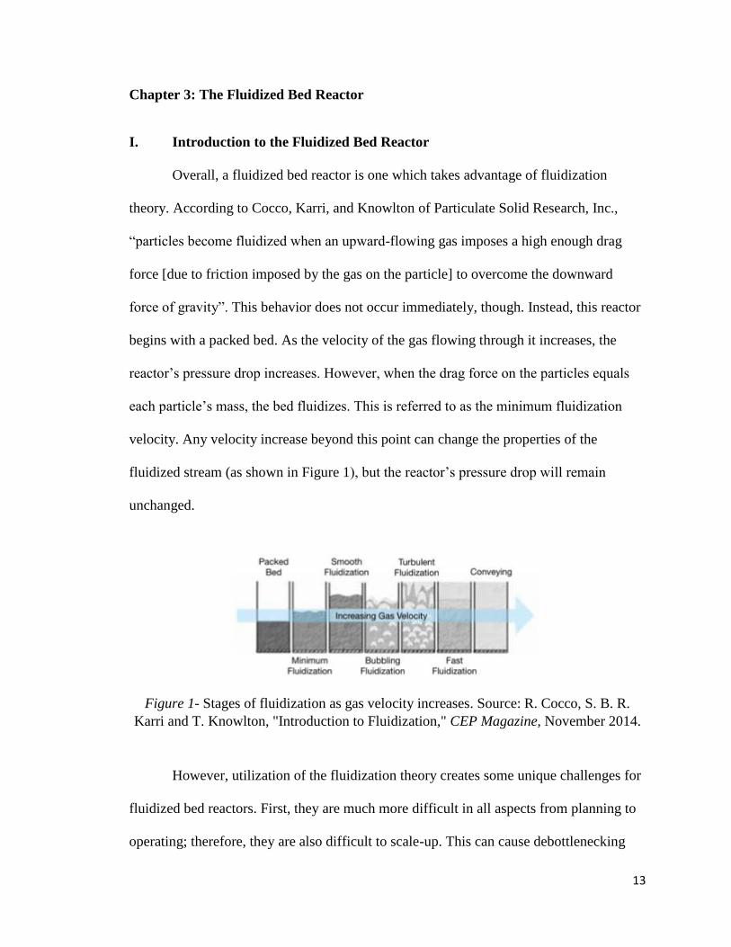
force of gravity”. This behavior does not occur immediately, though. Instead, this reactor

begins with a packed bed. As the velocity of the gas flowing through it increases, the

reactor’s pressure drop increases. However, when the drag force on the particles equals

each particle’s mass, the bed fluidizes. This is referred to as the minimum fluidization

velocity. Any velocity increase beyond this point can change the properties of the

fluidized stream (as shown in Figure 1), but the reactor’s pressure drop will remain

unchanged.

Figure 1- Stages of fluidization as gas velocity increases. Source: R. Cocco, S. B. R.

Karri and T. Knowlton, "Introduction to Fluidization," CEP Magazine, November 2014.

However, utilization of the fluidization theory creates some unique challenges for

fluidized bed reactors. First, they are much more difficult in all aspects from planning to

operating; therefore, they are also difficult to scale-up. This can cause debottlenecking

14

issues around the reactor if higher production is necessary. In addition, because the

catalyst is fluidized, some will be lost due to erosion or particle attrition. As this happens,

the company must pay to replace it, and this increased cost can accumulate significantly

over time.

Regardless of their challenges, though, fluidized bed reactors have several key

advantages over other reactor types due to their use of fluidization. First, the heat transfer

rate for a fluidized bed reactor is significantly higher than for other reactor types, like

packed beds, and this can be by as much as 5 to 10 times. This also allows the fluidized

bed to transfer heat produced in an exothermic reactor to a utility stream more efficiently;

therefore, it can effectively maintain an isothermal profile within a 5° allowance. In

addition, the fluidized catalyst allows for easy maintenance; therefore, catalyst can be

added or removed from the reactor without creating any downtime [2].

II. Given Values and Assumptions for a Fluidized Bed Reactor

Ultimately, a fluidized bed reactor can be simulated as an isothermal plug flow

reactor in Microsoft Excel and Pro/II software. To ensure that the reactor is actually

isothermal, the reactor contains a heat exchanger to supply the heat lost in the

endothermic reaction. In addition, because the catalyst bed is fluidized, a fraction of the

gas fed into the reactor will not react even with an infinite-sized reactor; as a result, this

fraction can be considered a bypass stream. Therefore, in all subsequent calculations, the

bypass is assumed to be 10 percent of the reactor feed.

Two primary constraints were also given regarding the operation of the fluidized

bed reactor. First, the fluidized bed reactor must operate within the appropriate

temperature range for the catalyst being used. In this case, the catalyst was assumed to

15

not have changed from the one used in the preliminary styrene process design; therefore,

the maximum temperature in the reactor is 1000 K. In addition, the minimum fluidization

velocity must be adjusted into the superficial gas velocity for the fluidized bed reactor

using a multiplier between 3 and 10.

At the beginning of the project, several values were also supplied regarding the

fluidized bed configuration. This first included specifications for the catalyst. Therefore,

in the following calculations and discussion, each catalyst particle is a sphere with a

diameter of 300 micrometers. These particles are 100 times smaller than the catalyst

particles utilized in the modelling of the isothermal and adiabatic reactors completed

previously. This gives the new catalyst a smaller void fraction, which is specified as 0.45

(the isothermal and adiabatic reactor catalyst had a void fraction of 0.5). This is

consistent with the fact that smaller particles can pack more efficiently, which means that

there will be less empty space between particles. However, it is not likely that the

difference in void fraction was the reason for using the smaller catalyst particles. Instead,

it is more likely that the catalyst was selected for the fluidized bed reactor because lighter

particles will fluidize easier.

In addition, specifications for the heat transfer tubes were provided. Therefore, in

the following discussion, each heat transfer tube is 20 feet long with a 25 mm diameter.

The overall heat transfer coefficient from the tubes to the heating medium is also defined

as 200 W/m2°C. In this project, the tube side stream is the utility; therefore, the length of

the tubes does not also define the length of the reactor.

Lastly, specifications for the fluidized bed reactor pricing were provided. This

included defining the installed cost of a fluidized bed reactor to be $10,000 per square

16

meter of heat transfer surface. Based on this definition, the installed cost of the reactor is

entirely dependent on the number of heat transfer tubes utilized. In addition, the bare

module factor for the reactor is 2.5.

III. Algorithm for Fluidized Bed Reactor Calculations in Excel

The following discussion describes the process to replace the isothermal packed

bed reactor with the fluidized bed reactor. The process was repeated to replace the

adiabatic packed bed reactor with the fluidized bed reactor. For the comparison between

the isothermal and fluidized bed reactors, the feed stream (which in Appendix B1 and B5

is shown as stream 9) has the same flowrate and composition as well as the same inlet

temperature and pressure of 550°C and 190 kPa, respectively. The actual comparison

between the reactor types will be focused on annual operating cost as well as outlet

stream composition and pressure drop. This section will only focus on the latter two.

As stated previously, it was assumed that 10 percent of the feed bypasses the

fluidized bed reactor; therefore, the first step of the calculations was to separate the 10

percent of bypass from the 90 percent of reactor feed. At this point, it was assumed that

the stream splits perfectly to keep the concentrations of all components (including water,

ethylbenzene, styrene, benzene, and toluene) the same in both the bypass and the feed

stream.

Next, it was assumed that the process would contain 1 large reactor with a volume

of 250 cubic meters (equal to the entire catalyst volume). This was an arbitrary decision

that could easily be changed to multiple reactors in parallel with smaller, equal volumes.

Because the composition of the reacting stream changes as it progresses through the

reactor, calculations were done for 10 reactor intervals of 25 cubic meters each. Also,

17

because this was simulated in Excel, complicated and more realistic thermodynamic

packages were not able to be utilized; therefore, it was assumed that the ideal gas law

applied to all streams in the process.

To continue the calculations investigating the outlet stream composition and the

pressure drop, the change in the number of moles of each component per hour was first

able to be tabulated using the 4 reaction rate laws given previously in the project

assignment (shown in Appendix D1). Because the steam present in the reactor was a

diluent, the number of moles of water in the reactor was constant. This determined the

pressure increase for each reactor interval due to an increase in the number of moles in

the reactor. However, this pressure increase was ultimately countered and overcome by a

larger pressure drop calculated using the Ergun equation.

The Ergun equation requires the length of each reactor interval. However, the

actual dimensions of the reactor were originally unknown and needed to be calculated. In

order to achieve this, the calculations described next were completed with the assumption

that, for each of the reactor intervals, the inlet stream defined properties such as the

density of each component as well as the minimum fluidization velocity of the reacting

stream. Based on these assumptions, the length and cross-sectional area of the reactor

varied with each interval.

The calculations to determine reactor length can be split into two smaller

subsections with distinct goals. Ultimately, the first goal was to determine the superficial

gas velocity in the reactor. This first required determination of the minimum fluidization

velocity in the reactor, which could be simply calculated using the Archimedes and

Reynolds numbers (shown in Equations 1 and 2).

18

𝐴𝑟 =𝑑𝑝

3(𝜌𝑠 − 𝜌𝑔)𝜌𝑔𝑔

𝜇𝑔2

𝑅𝑒 =𝑢𝑚𝑓𝑑𝑝𝜌𝑔

𝜇𝑔= [1135.69 + 0.0408𝐴𝑟]0.5 − 33.7

Equation 1 and 2- Equations for the Archimedes number and Reynolds number. In this

case, Ar is the Archimedes number, Re is the Reynolds number, dp is the particle

diameter, ρs is the catalyst density, ρg is the gas density, μg is the gas viscosity, and g is

the acceleration due to gravity.

Upon closer investigation, it was clear that only one variable required for these

equations was absent from the project description: the density of the reacting gas. To find

this, the ideal gas law was first required to determine the density in each interval of each

component in the reacting stream. Then, the overall gas density in the reactor interval was

calculated using a weighted average. Once the minimum fluidization velocity in each

interval was determined, it required adjustment using a multiplier to determine the

superficial velocity of the gas. As stated previously, this multiplier must be between 3

and 10; therefore, for these calculations, the value of 6.5 was arbitrarily selected as it is

exactly in the middle of the available range.

The second goal was to determine the reactor’s cross-sectional area and length.

This was done using the volumetric flowrate, which was calculated using the ideal gas

law for each interval. Then, knowing the superficial gas velocities calculated previously,

the cross-sectional area for each interval was calculated. This was then used to find the

length based on a reactor volume of 250 cubic meters.

Ultimately, these calculations resulted in 11 different possibilities for the reactor’s

length and cross-sectional area due to the 11 different superficial velocities calculated.

19

However, the length, cross-sectional area, and superficial velocity calculated for the final

interval (right before the stream exits the reactor) was selected for the entire reactor

because it allows the accommodation of the largest volumetric flowrate of reacting gas.

These values satisfy the variables of the Ergun equation which had not been supplied in

the project description.

IV. The Selection of the Fluidized Bed Reactor Configuration

Completing the calculations discussed in the previous section ultimately resulted

in a fluidized bed reactor with a cross-sectional area of 198 m2 and a length of 1.3 meters.

The stream passing through this reactor also experienced a pressure drop of 56.5 kPa

(from 190 to 133.5 kPa). Overall, this pressure drop was not unreasonable. This was

because, in previous calculations completed during the styrene optimization project, the

pressure of the stream leaving the reactor section could be as low as approximately 110

kPa without negatively impacting the process’s performance. This can be seen in stream

12 (shown in Appendix B5) in the optimized styrene process with the adiabatic reactors.

However, the large cross-sectional area of 198 m2 (and therefore a diameter of

nearly 16 meters) was cause for alarm in this case. This diameter is approximately twice

as large as the diameter of each individual large tower in the T-502 scheme. In the base

case (with isothermal reactors), each tower with T-502 specifications had a diameter of

7.1 m. Likewise, Appendix B8 showed that in the optimized case (with adiabatic

reactors), each T-502 tower had a diameter of 9.0 m. As a result, the reactor’s large

diameter seemed unreasonable in comparison.

The only reasonable remedy to the issue with the large reactor diameter was to

split it into multiple reactors with smaller, equal volumes (which sum to the 250 m3

20

required) in parallel. If there were 2 reactors in the scheme, each would have a volume of

125 m3 and handle 45% of the stream 9 flowrate. Completing the previously discussed

calculations with these values gave each reactor a cross-sectional area of 99.2 m2, which

means that the diameter of each was 11.2 m. This is still larger than the diameters in the

T-502 scheme.

Therefore, a scheme with 3 reactors needed to be investigated. If there were 3

reactors, each would have a volume of 83.3 m3 and handle 30% of the stream 9 flowrate.

These values resulted in each reactor having a cross-sectional area of 66.1 m2. This

means that the diameter for each reactor was 9.2 m, which is very close to the diameter of

the towers in the T-502 scheme. Therefore, the configuration with 3 fluidized bed

reactors in parallel was selected, and it maintained the same length and pressure drop as

the one large fluidized bed reactor. In addition, it was assumed that the fluidized bed

reactors used nC36 as a utility to maintain an isothermal profile. This allowed the number

of tubes required in each reactor to be calculated.

21

Chapter 4: Comparing Reactor Types Based on EAOCs

Overall, in order to determine which reactor (isothermal, adiabatic, or fluidized

bed) was best for the styrene production process, it was necessary to define the

quantitative metric by which the 3 would be compared. In this project, it was possible

that net present value (NPV) could have been chosen, as this was the metric previously

utilized during process optimization. However, a simpler metric to use was the equivalent

annual operating cost, or EAOC, which takes into account only the reactor and its

associated utility streams.

In order to calculate the EAOC of each reactor, it was first necessary to calculate

the capital investment associated with each reactor scheme. In the case of the isothermal

and adiabatic reactors, there were 2 schemes with 5 reactors each. This is shown as R-

501a-e and R-502a-e for isothermal reactors in Appendix B1 and R-503a-e and R-504a-e

for adiabatic reactors in Appendix B5. This was then plugged into the capital recovery

equation shown below (the capital investment is the present value, or P variable) to find

the annual equivalent of the capital investment. This assumed that the capital investment

could be modelled as an equal payment series. For the styrene production process, the

plant life (N) is 12 years and the interest rate (i) is 12 percent.

𝐴 = 𝑃 [𝑖(1 + 𝑖)𝑁

(1 + 𝑖)𝑁 − 1]

Equation 3- The capital recovery equation where the capital investment is the present

value (P). In this case, i is the interest rate and N is the plant life.

Then, the yearly operating cost for each reactor was determined. In this case, it

was assumed that there was no annual cost for the refrigerant nC36 used by the

22

isothermal and fluidized bed reactors. Therefore, only the utility which provided the

energy for the reactor- in this case, the natural gas used in the fired heater- needed to be

taken into account. Because this was already on a yearly basis, no adjustment needed to

be made to it.

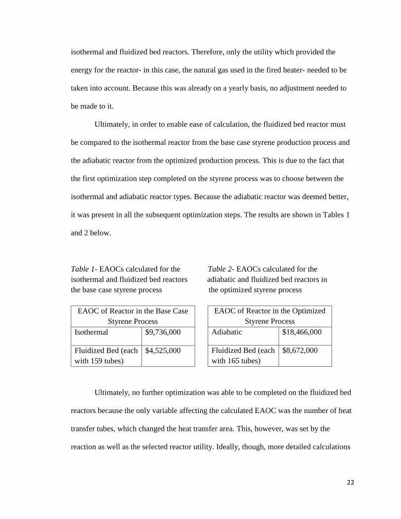
Ultimately, in order to enable ease of calculation, the fluidized bed reactor must

be compared to the isothermal reactor from the base case styrene production process and

the adiabatic reactor from the optimized production process. This is due to the fact that

the first optimization step completed on the styrene process was to choose between the

isothermal and adiabatic reactor types. Because the adiabatic reactor was deemed better,

it was present in all the subsequent optimization steps. The results are shown in Tables 1

and 2 below.

Table 1- EAOCs calculated for the Table 2- EAOCs calculated for the

isothermal and fluidized bed reactors adiabatic and fluidized bed reactors in

the base case styrene process the optimized styrene process

EAOC of Reactor in the Base Case

Styrene Process

Isothermal $9,736,000

Fluidized Bed (each

with 159 tubes)

$4,525,000

Ultimately, no further optimization was able to be completed on the fluidized bed

reactors because the only variable affecting the calculated EAOC was the number of heat

transfer tubes, which changed the heat transfer area. This, however, was set by the

reaction as well as the selected reactor utility. Ideally, though, more detailed calculations

EAOC of Reactor in the Optimized

Styrene Process

Adiabatic $18,466,000

Fluidized Bed (each

with 165 tubes)

$8,672,000

23

for the EAOC would allow the velocity multiplier, the reactor utility, and the reactor inlet

temperature and pressure to be optimized.

It was very clear based on the simplified calculations that the fluidized bed

reactors were the best option to minimize the reactor cost in the styrene production

process. This was most likely due to the fact that the 3 fluidized bed reactors could take

the place of 10 isothermal or adiabatic reactors; therefore, they greatly reduced the capital

investment for the reactors. Ultimately, the requirement of fewer actual reactors in the

process was due to the fact that, by virtue of the fluidized process stream, the fluidized

bed reactors have more efficient heat transfer.

However, it must be noted that, while the EAOC of the adiabatic reactors is larger

than that of the isothermal reactors, isothermal reactors are not necessarily better. This is

due to the fact that adiabatic reactors actually have a higher yield of styrene from

ethylbenzene (58 percent for adiabatic reactors versus 50 percent for isothermal). This

resulted in a decrease in the cost of raw materials which counteracted and overcame the

increased reactor cost. Ultimately, this shows that, in order to be more definitive about

which reactor was superior, it would be better to create a clearer comparison between the

three. This could be done by setting the conversion or selectivity within the reactors

constant and solving for the equivalent annual operating cost again. In addition, it would

likely be better to compare the net present value of the optimized styrene process with the

different reactor types implemented. Without time constraints, these would be the next

steps to continue the project.

24

Chapter 5: Conclusion

Ultimately, this thesis began with a discussion about chemical engineering design,

process optimization, and simulation. These were necessary to complete the ChE 451

design project, which was to create an optimized styrene process given a base case.

During the design project, isothermal and adiabatic reactors were investigated. However,

this work was expanded upon by investigating fluidized bed reactors as an alternative.

The theory behind fluidized bed reactors was discussed before the fluidized bed

reactor calculations were detailed. Overall, the fluidized reactor was simulated in

Microsoft Excel. The calculation algorithm can be summarized with three main

equations: the Archimedes and Reynolds number equations (which helped to calculate

the minimum fluidization velocity in the reactor) and the Ergun equation (which

determined the reactor’s pressure drop along its length). In the end, these calculations

resulted in a scheme of 3 fluidized bed reactors with volumes of 83.3 m3 in parallel.

Lastly, the equivalent annual operating costs (EAOCs) of the isothermal,

adiabatic, and packed bed reactors were calculated. When compared to the isothermal and

adiabatic reactors, the fluidized bed reactors were found to have approximately half the

associated costs. This was likely because the fluidized bed reactor scheme only contained

three reactors while the isothermal and adiabatic schemes each contained ten; therefore,

the capital investment required for the fluidized bed reactors is much smaller. However,

these calculations were greatly simplified. As a result, to get a more accurate picture of

the reactor comparison, the conversion or selectivity in all the reactors should be set

constant and the EAOCs should be calculated again. The net present value of the styrene

process with the different reactor types could also be compared.

25

Appendices

26

Appendix A – Styrene Process Optimization Design Report (written

with Seth Gray and Mitch Sypniewski in ChE 451, Fall 2018)

I. Introduction

Landshark Inc. is considering implementing a styrene production process at its

OM petrochemical facility. The proposed process utilizes the dehydrogenation of

ethylbenzene to produce 100,000 tonnes of styrene per year with at least 99.5 weight

percent purity. Landshark Inc. will sell the styrene to manufacturers interested in

polymerizing it to make polystyrene packaging and foam insulation, which could

potentially be profitable.

Our engineering team received a preliminary design and was instructed to first

complete a base case analysis and determine economic feasibility. We found that the

plant had a net present value (NPV) of -$320.3 M. Because this NPV is negative, our

team will require information about the other sections of the plant (such as a styrene

polymerization section, if it exists) to make an accurate recommendation regarding the

project. Assuming a later section of the OM facility does polymerize 100,000 tonnes of

styrene per year, the NPV based on buying the styrene at market value is -$1.4 B;

therefore, under these conditions, Landshark Inc. should pursue the project further even

in its current form. If Landshark Inc. does not polymerize styrene, though, they should

not pursue the project further with the current design as it would only increase company

debt.

After completing base case analysis, we then investigated changes proposed by

management as well as other optimizations as we saw fit. These changes gave the plant

an NPV of $31 M, which indicates that the updated design can turn a profit and the

27

project should undergo further consideration regardless of whether or not the OM facility

polymerizes styrene.

II. Base Case

Our engineering team modeled the base case of Landshark, Inc.’s preliminary

design in Microsoft Excel. We simulated the same design in Pro/II to utilize more

complicated and realistic thermodynamic relationships in our calculations. We then

compared those results to the Excel simulation, which assumed that the streams behave as

ideal gases and solutions. In Pro/II, we used the SRK-SimSci thermodynamic model

based on the path our system follows in the thermodynamic flowsheet (see Appendix

C11). The tower T-502 scheme, however, was simulated using the ideal thermodynamic

method.

Our team found that the preliminary design as given to us by management had a

NPV of -$320.3 M and an annual equivalent (AE) of -$51.7 M with a 12% minimum

acceptable rate of return (MARR). This results in both a conventional and a discounted

payback period greater than 12 years. Because the project had a negative NPV and a

payback period longer than the project life, the project is not profitable with the

preliminary design. However, with changes it could become more lucrative.

After inspection, several process parameters fell outside of normal operating

conditions defined in Analysis, Synthesis, and Design of Chemical Processes by Turton et

al. We then analyzed whether each of these conditions was justified. First, moving

sequentially through the plant, reactors R-501 and R-502 had both high temperature and

non-stoichiometric feed. These are justified because the steam present in the feed

improves reactor conversion and provides heat to both fuel the reaction and keep all

28

components in the gas phase. The low pressure of the towers T-501 and T-502 and the

vessels V-502 and V-503 are justified by the need of a gas phase for vapor-liquid

equilibrium and the lack of pumps or valves between the towers and vessels. The large

log mean temperature differences of heat exchangers E-501, E-502, E-503, and E-505 are

justified because the utilities defined in the base case (either high pressure steam or

cooling water) are required to vaporize or cool each exchanger’s respective stream.

Compressor C-501 also has a pressure ratio of 6; however, unlike the previous

parameters, this is not justified and must be changed for the optimized case.

Finally, we utilized sensitivity analysis (shown in Appendix C1) to determine

which parameters had the greatest effect on NPV. As can be seen in the figure, the

styrene price and the raw materials cost varied the most. Due to this observation, we

decided to focus on reducing the raw materials cost.

III. Notes about Sign Conventions for Optimization

The engineering team used discrete optimization when trying to make

improvements to the styrene production process. When referring to an increased cost, the

NPV contribution is becoming more negative.

IV. First Change: Reactor Type

The first change we investigated was replacing the original isothermal reactors

with adiabatic reactors. We treated isothermal reactors as heat exchangers, since the

reacting stream will only undergo a pressure drop within the reactor. We also treated

adiabatic reactors as vessels, since the reacting stream will undergo both a temperature

and a pressure drop within the reactor. Ultimately, the objective in doing this was to

decrease the raw materials cost by increasing the overall yield of styrene.

29

Appendix C2 shows an economic comparison of the process after implementing

each type of reactor. Notice that the inlet temperature of the adiabatic reactor R-503 is

25°C lower in comparison to the original isothermal reactor. This adjustment was made

because preliminary design conditions stipulated that the temperature drop in each reactor

must be less than 50°. The choice of 525°C resulted in a temperature drop of 49.86°.

Lowering the temperature further would result in a lower NPV because it increases the

fixed capital investment as well as the annual cost of raw materials and utilities. Overall,

these changes improved the NPV by approximately $56 M. Appendix C2 shows the

breakdown of the most notable cost contributions (raw materials, utilities, and fixed

capital investment).

The largest contribution to the improved NPV was the decrease in the cost of raw

materials. This was due to a lower single pass conversion of ethylbenzene in the reactor

section (57% to 42%), which ultimately resulted in a larger ethylbenzene recycle stream

and a higher overall yield of styrene (50% to 58%). The elimination of the original

isothermal reactor also increased NPV by saving approximately $2 M in heating utility

costs. The almost 4,800 kmol/hr increase in the steam utility required to heat the reactor

R-503 effluent (stream 12) to the inlet temperature of R-504 counteracted but did not

overcome the cost savings.

The contribution of the FCI to the project’s NPV is primarily attributed to three

different points in the process. Firstly, the adiabatic reactors R-503 and R-504 have larger

equipment equipment cost attributes, which are related to capacity and are reported in

square meters for heat exchangers and cubic meters for vessels. In this process, the vessel

volume is the same as the catalyst volume- 50 m3 - while the heat exchanger area required

30

is smaller (and it stores the required volume of catalyst in its shell.) Therefore, the

equipment with the larger equipment cost attributes (in this case, the vessels) is more

expensive. Second, the duty (and therefore the size) of the fired heater increases when the

process implements an adiabatic reactor. This is due to the increased steam utility in heat

exchanger E-503. Lastly, the cost of the tower T-502 scheme increases because the

number of towers required increases from 4 to 5. This is due to the lower single pass

conversion of ethylbenzene in the reactor sections; therefore, this leaves a larger amount

of ethylbenzene present in T-502, and the higher flowrate requires a larger tower volume.

Overall, this decision is based on a comparison between the preliminary

isothermal reactor and the optimized adiabatic reactor. If given more time, the

engineering team would pursue optimization of the isothermal reactor for a more

thorough decision concerning which reactor type is preferable.

V. Second Change: Reactor Conditions

The second change we investigated was changing the volume and pressure of

reactor R-503 and the volume of R-504. Similarly to the change from isothermal to

adiabatic reactors, the objective in doing this was to decrease the raw materials cost (by

increasing the overall yield of styrene). Overall, these changes improved the NPV by

approximately $60 M. A breakdown of the most notable cost contributions (raw

materials, catalyst, utilities, and fixed capital investment) is shown in Appendix C3.

The most significant change in the reactor scheme was adjusting the volumes of

R-503 and R-504 from 50 to approximately 36 m3. In both reactors this resulted in a

slight decrease in single-pass conversion and an increase in the selectivity of

ethylbenzene, as seen in Appendices B4-B7. The changes in conversion and selectivity

31

ended up increasing the yield of styrene from the reactors (from 58% to 68%). This in

turn decreased the required feed of ethylbenzene by 28.4 kmol/hr, which ultimately

decreased the raw materials cost by $22 M per year. Since the catalyst volume is

proportional to the reactor volume, this change accompanied a decrease in the catalyst

cost of $2.5 M per year.

An insignificant change made to the reactor scheme was changing the inlet

pressure to R-503 from 190 to 187.5 kPa. This only increased the NPV by approximately

$1 M due to the given rate law equations, which are in terms of partial pressures.

VI. Third Change: Materials of Construction

The third investigation was on the materials of construction of the towers and

reactors. The preliminary tower design specified using titanium, which is very expensive.

Carbon steel is usable at the towers’ operating conditions (vacuum pressures and

T<125°C) and is about 11% the cost of titanium. The outsides of the towers will need to

be epoxied or painted to prevent atmospheric corrosion.

The base case reactors were made of 316 stainless steel which is susceptible to

hydrogen embrittlement and hydrogen blistering. This is where atomic hydrogen diffuses

into a dislocation in a metal and bonds with another atomic hydrogen to form a gas. The

gas expands and damages equipment, causing it to need to be replaced more frequently

[3]. Due to the mechanism of ethylbenzene dehydrogenation, atomic hydrogen will be

present in the reactors. We changed the material of construction to nickel alloy clad,

which is less susceptible to hydrogen embrittlement and hydrogen blistering, since it is

also operable under the reactors’ conditions (T<600°C and P<200 kPa). This change

32

slightly decreased the NPV by increasing the FCI. This occurred because nickel alloy

clad is more expensive than stainless steel.

Ultimately, changing the material of construction of the towers and reactors

increased our NPV by $165 M. The main contribution to this was a decrease in the FCI

because the decreased tower cost greatly outweighed the increased reactor cost, as shown

in Appendix C8.

VII. Fourth Change: Extra Tower to Purify Benzene Stream

The fourth change that was analyzed was the addition of a benzene/toluene

distillation tower (T-503). The benzene and toluene byproduct stream entered T-503 at

50°C and 200 kPa. Tower T-503 separated the benzene and toluene to deliver benzene

with 99.5 mole percent purity to the bottoms. With this high purity, Landshark Inc. could

sell the benzene at full price, therefore increasing the revenue of the plant from $239 M

to $253 M. This outweighs the $0.5 M decrease in FCI. This ultimately increased NPV

by $56 M.

VIII. Fifth Change: Heat Integration

Due to the recent decrease in the market value of utilities, the engineering team

only focused on implementing heat integration in one section of the process. In the

preliminary design, high pressure steam (HPS) heated and vaporized stream 2 in heat

exchanger E-501. The effluent from reactor R-502, or stream 12, flowed directly into heat

exchanger E-503 where it cooled through interaction with cooling water (CW) and exited

as stream 13. The preliminary design PFD (Appendix B1) shows this setup.

33

The proposed changes shown in the optimized design PFD (Appendix B5)

resulted in an elimination of the HPS utility in E-501 and a reduction in the CW required

in E-503. In the new design, the effluent stream 12 from reactor R-504 (previously called

R-502 in the base case) redirects to the utility side of E-513 (previously E-501). Since it

now serves as the heating fluid, its temperature decreases in the heat exchanger and exits

as stream 36. This flows into E-503 where it cools further to become stream 13. Overall,

this improved the NPV by approximately $4 M. Appendix C9 shows the breakdown of

the most notable cost contributions (raw materials, utilities, and fixed capital investment).

IX. Sixth Change: Compressor Adjustments

In the base case, the pressure ratio across compressor C-501 was 6. For safe

operating conditions the pressure ratio needed to be decreased to below 3. To achieve

this, the engineering team looked into using multi-stage compression. When adding a

second compressor (C-502) with an interstage cooler, the pressure ratio decreased to

approximately 2.45 across both C-501 and C-502. We accepted this change because it is

under the threshold for safe operation. With the addition of a second compressor (C-502)

and a heat exchanger (E-512), the utilities and FCI decreased compared to the base case.

This increased the NPV by $11 M.

X. Summary

The economic data for the optimized case results in an NPV of $31 M, a

discounted cash flow rate of return (DCFROR) of 16%, and an annual equivalent (AE) of

$4.93 M. Provided below in Appendix C10 is a comparison of the optimized case and the

base case. The DCFROR for the base case has been marked as N/A since it could not be

calculated.

34

XI. Process Safety Considerations

Overall, one of the main concerns for process safety will be keeping high

temperature vapors and steam away from employees. If exposure to high temperature

lines is likely, maintenance staff and operators should wear proper PPE. Otherwise,

during the design process, engineers can protect employees by consciously attempting to

put high temperature process and steam lines away from expected high traffic areas. In

addition, the temperatures throughout the process are higher than the flash points of each

component. Therefore, there will need to be measures put into place to avoid ignition

sources. Also, since the reaction is endothermic, runaway reactions will not be a concern.

However, isolating the reactors, where temperatures of the streams are extremely high,

would also be advisable. This alleviates the danger of burns if there is a rupture in piping

or equipment.

The other main process safety concern noted was limiting exposure to the

chemicals in the process. In the case of a spill, people exposed to high concentrations of

chemical vapor must use self-contained respiratory devices because components in the

process can act as lung irritants and asphyxiants. Also, proper ventilation should be in

place in all areas where spills are likely to occur.

XII. Sensitivity Scenarios

The three parts of this process that were most susceptible to change were the

prices of ethylbenzene, styrene, and utilities; therefore, the team focused on formulating

scenarios for changes in these variables. The following changes would affect the

optimized case defined above.

35

First, the team investigated ethylbenzene and styrene scenarios. If the price of

ethylbenzene decreases, then the team would not have to focus so much on maximizing

the overall yield of styrene. Also, if the price of ethylbenzene increases or the price of

styrene decreases, it might not be profitable to produce the styrene. It may be better to

simply purchase the styrene. Lastly, if the price of styrene increases, the profitability of

producing the styrene on-site would increase.

In addition, utility costs are susceptible to change. If the cost of utilities were to

increase, heat integration would need further investigation and implementation. This

would allow the plant to minimize necessary utilities. If the cost of utilities were to go

down, little would change in the optimized design process.

XIII. Conclusions

Given specifications of 100,000 tonnes of styrene produced per year with a purity

of at least 99.5 wt%, the engineering team determined the economic viability of

producing styrene from the dehydrogenation of ethylbenzene. The NPV of the base case

was -$320.2 M.

However, after the proposed changes, the NPV of the optimized case was $31 M.

Therefore, we recommend the optimized case undergo further investigation and

optimization. Our recommendations include investigating different inlet temperatures and

pressures in tower T-503, adding more heat integration, and improving vessel V-501.

After finishing optimization, Landshark Inc. could begin to discuss options for buying the

process equipment from contractors, thus reducing the design inaccuracy due to the

pricing calculations.

36

Appendix B- Base and Optimized Case Specifications

1. Base Case PFD

Figure 1: Base case process flow diagram as given in the problem statement

37

2. Base Case Stream Table

Table 1: Base case stream table as calculated for ChE 451 (all flowrates are in kmol/h)

Stream No. 1 2 3 4 5 6 7 8 9

Temperature (°C) 136 117 225 159 800 800 800 800 550

Pressure (kPa) 205 205 190 600 565 565 565 190 190

Vapor Mole Fraction 0 0 1 1 1 1 1 1 1

Total Flow (kg/h) 26430 45962 45962 90742 90742 28288 62454 62454 108416

Total Flow (kmol/h) 250 434 434 5037 5037 1570 3467 3467 3901

Comp. Flow (kmol/h)

Water 0 0 0 5037 5037 1570 3467 3467 3467

Ethylbenzene 245 427 427 0 0 0 0 0 427

Styrene 0 1.2 1.2 0 0 0 0 0 1.2

Hydrogen 0 0 0 0 0 0 0 0 0

Benzene 2.5 2.5 2.5 0 0 0 0 0 2.5

Toluene 2.5 3.1 3.1 0 0 0 0 0 3.1

Ethylene 0 0 0 0 0 0 0 0 0

Methane 0 0 0 0 0 0 0 0 0

Stream No. 10 11 12 13 14 15 16 17 18

Temperature (°C) 550 575 575 270 180 65 65 65 65

Pressure (kPa) 180 165 147 132 117 102 102 102 102

Vapor Mole Fraction 1 1 1 1 1 0 1 0 0

Total Flow (kg/h) 108416 108416 108416 108416 108416 108416 3738 43077 61600

Total Flow (kmol/h) 4023 4023 4080 4080 4080 4080 219 442 3419

Water 3467 3467 3467 3467 3467 3467 47 0 3419

Ethylbenzene 273 273 186 186 186 186 0.9 185 0

Styrene 98 98 121 121 121 121 0 121 0

Hydrogen 64 64 58 58 58 58 56 1.5 0

Benzene 28 28 62 62 62 62 2.1 60 0

Toluene 35 35 65 65 65 65 0.8 64 0

Ethylene 25 25 60 60 60 60 51 8.4 0

Methane 32 32 62 62 62 62 59 2.7 0

Stream No. 19 20 21 22 23 24 25 26 27

Temperature (°C) 227 65 50 121 91 123 700 50 123

Pressure (kPa) 240 60 40 60 25 55 555 200 200

Vapor Mole Fraction 1 0 0 0 0 0 1 0 0

Total Flow (kg/h) 5354 43077 9430 32032 19532 12500 28288 9430 12500

Total Flow (kmol/h) 247 442 110 304 184 120 1570 110 120

Water 47 0 0 0 0 0 1570 0 0

Ethylbenzene 1.0 185 1.8 183 182 0.6 0 1.8 0.6

Styrene 0 121 0 121 1.2 119 0 0 119

Hydrogen 58 1.5 0 0 0 0 0 0 0

Benzene 14 60 49 0 0 0 0 49 0

Toluene 5.5 64 59 0.6 0.6 0 0 59 0

Ethylene 59 8.4 0 0 0 0 0 0 0

Methane 62 2.7 0 0 0 0 0 0 0

Stream No. 28 29 30 31

Temperature (°C) 65 91 50 63

Pressure (kPa) 200 205 40 40

Vapor Mole Fraction 0 0 1 1

Total Flow (kg/h) 61600 19532 1615 5354

Total Flow (kmol/h) 3419 184 29 247

Water 3419 0 0 47

Ethylbenzene 0 182 0 1.0

Styrene 0 1.2 0 0

Hydrogen 0 0 1.5 58

Benzene 0 0 11 14

Toluene 0 0.6 4.7 5.5

Ethylene 0 0 8.2 59

Methane 0 0 2.7 62

38

3. Base Case Process Description

Fresh liquid ethylbenzene at 136°C and 205 kPa (stream 1) is combined with a

recycle of liquid ethylbenzene (stream 29) to form a feed mixture (stream 2). This then

enters heat exchanger E-501 which utilizes high pressure steam to vaporize the stream

and increase its temperature to 225°C (stream 3). The stream experiences a pressure drop

of 15 kPa through the heat exchanger, which is typical of all of the heat exchangers in the

process. The vaporized stream 3 is mixed with an adequate amount of high-pressure

steam (stream 8) to form stream 9. This stream is then fed to reactor R-501a-e at a

temperature of 550°C and a pressure of 190 kPa. The reactor consists of a catalytic bed

and has 4 reactions that occur:

For the equations above, pi is the partial pressure of component I in Pa, T is the

temperature in K, the activation energy is in J/mol, and the rate is in mole/(m3 catalyst *

second).

The effluent (containing ethylbenzene, styrene, hydrogen, benzene, ethylene,

toluene and methane) coming from the reactor at 550°C and 179.9 kPa (stream 10) is

then sent to a heat exchanger E-502 that increases the temperature to 575°C. Stream 11

coming from E-502 enters the second reactor R-502a-e and undergoes the same reactions

shown previously. The 8-component vapor stream exiting the reactor (stream 12) is fed to

39

a series of three heat exchangers (E-503, E-504, and E-505, which use high pressure

steam, low pressure steam, and cooling water utilities respectively). Here the vapor is

cooled and partially condensed into a liquid/vapor mixture at 65°C and 102.2 kPa (stream

15). This mixture is then fed to a 3-phase separator, V-501, where it separated into three

streams: the vapor stream (stream 16), containing all the aqueous and organic

components in the inlet stream, the organic liquid stream (stream 17), and a water stream

(stream 18). The vapor stream is mixed with the fuel gas coming out of reflux drum V-

502 (stream 30) to form stream 31. Stream 31 is then fed to compressor C-501 which

increases the temperature and pressure to 227°C and 240 kPa (stream 19). These are the

conditions at which the stream is sold as fuel gas. The water stream is fed to pump P-

501A/B where the pressure is increased to 200 kPa and treated as wastewater. The

organic liquid stream goes through a valve and comes out at 60 kPa (stream 20). Stream

20 is then fed onto tray 4 of the first tower T-501, which has 18 stages and operates at

65°C and between 40 and 60 kPa. This tower has a reboiler, E-506, which uses a low-

pressure steam utility. The column produces a bottoms stream (stream 22) which recovers

1% of the toluene and 99% of ethylbenzene in stream 20.

The vapor stream from the top of T-501 is condensed in heat exchanger E-507

using cooling water and sent to Reflux Drum V-502. Here the vapor and liquid phases are

separated into streams 30 and 21 respectively. The vapor stream 30 is combined with the

fuel gas. The liquid benzene/toluene byproduct (stream 21) is sent to pump P-504A/B

where the pressure is increased to 200 kPa. Stream 22 (bottoms product from T-501) is

fed to tray 28 of T-502 where further separation is accomplished. T-502 contains 68 total

stages, and it operates between 25 and 55 kPa. It also has a reboiler (E-508), which uses

40

low pressure steam. The vapor product from the top of the T-502 condenses in heat

exchanger E-509, using cooling water, before it goes through reflux drum V-503. The

liquid stream then goes through pump P-503A/B where its pressure decreases to 25 kPa

(stream 23). Stream 23 is then sent through P-506A/B where the pressure is increased to

205 kPa before it is recycled and combined with stream 1. The bottoms of T-502 in

stream 24 are sent to P-505A/B where it undergoes a pressure increase to 200 kPa to

become stream 27. This is the final pure styrene product (with a 99.5 mass percent purity)

flowing at a rate of 100,000 tonnes per year.

The only other inlet stream is low pressure steam fed to the fired heater H-501 at

159°C and 600 kPa (stream 4). It is heated in H-501 to 800°C in stream 5 where it is then

split into streams 6 and 7. Stream 7 goes through a valve where there is a 375 kPa

pressure drop before going into stream 8 which combines with stream 3. Stream 6 is fed

to heat exchanger E-502 and is used to heat the first reactor effluent (stream 10) to

575°C.

41

4. Optimized Case Process Description

Fresh liquid ethylbenzene at 136°C and 205 kPa (stream 1) is combined with a

recycle of liquid ethylbenzene (stream 29) to form a feed mixture (stream 2). This then

enters heat exchanger E-513 which utilizes stream 12 from reactor to vaporize the stream

and increase its temperature to 225°C (stream 3). The stream experiences a pressure drop

of 15 kPa through the heat exchanger, which is typical of all of the heat exchangers in the

process. The vaporized stream 3 is mixed with an adequate amount of high-pressure

steam (stream 8) to form stream 9. This stream is then fed to reactor R-503a-e at a

temperature of 525°C and a pressure of 187.5 kPa. The reactor consists of a catalytic bed

and has 4 reactions that occur:

The effluent (containing ethylbenzene, styrene, hydrogen, benzene, ethylene,

toluene and methane) leaves the reactor at 483°C and 164 kPa (stream 10). It is then sent

to heat exchanger E-502 where the temperature increases to 575°C. Stream 11 coming

from E-502 enters the second reactor, R-504a-e, and undergoes the same reactions shown

previously. An 8-component vapor stream exits the reactor (stream 12) and is then used

as the utility in E-513. Stream 12 goes through E-513 and become stream 36 which is fed

to a series of three heat exchangers (E-503, E-504, and E-505, which use high pressure

steam, low pressure steam, and cooling water utilities respectively). Here the vapor is

cooled and partially condensed into a liquid/vapor mixture at 65°C and 68 kPa (stream

15). This mixture is then fed to a 3-phase separator, V-501, where it separated into three

streams: the vapor stream (stream 16), containing all the aqueous and organic

components in the inlet stream, the organic liquid stream (stream 17), and a water stream

(stream 18). The vapor stream is mixed with the fuel gas coming out of reflux drum V-

42

502 (stream 30) to form stream 31. Stream 31 is then fed to compressor C-501 which

increases the temperature and pressure to 157°C and 98 kPa (stream 34). Stream 34 is

sent to an interstage cooler E-512 where it cools the stream to 63°C (stream 35). Stream

35 is then fed to compressor C-502 where its temperature and pressure are increased to

157°C and 240 kPa (stream 19). These are the conditions at which the stream is sold as

fuel gas in stream 19. The water stream (stream 18) is fed to pump P-501A/B where the

pressure is increased to 200 kPa and treated as wastewater. The organic liquid stream

goes through a valve and comes out at 60 kPa (stream 20). Stream 20 is then fed to tower

T-501 which has 32 stages and operates at 65°C and between 40 and 60 kPa. This tower

has a reboiler, E-506, which uses a low-pressure steam utility. The column produces a

bottoms stream (stream 22) which recovers 1% of the toluene and 99% of ethylbenzene

in stream 20.

The vapor stream from the top of T-501 is condensed in heat exchanger E-507

using cooling water and sent to Reflux Drum V-502. Here the vapor and liquid phases are

separated into streams 30 and 21 respectively. The vapor stream 30 is combined with the

fuel gas. The liquid benzene/toluene byproduct (stream 21) is sent to pump P-504A/B

where the pressure is increased to 200 kPa (stream 26). Stream 26 is then fed to tower T-

503 where the overhead product (Stream 32) is 99.5 mole % benzene. The overhead is

condensed in exchanger E-511 and sent to Reflux Drum V-504. After V-504 the stream is

sent through pump P-507A/B where stream 32 is sold as benzene. The bottoms for T-503

is the Toluene stream in stream 33 that is sold. The reboiler for tower T-503 is E-510.

Stream 22 (bottoms product from T-501) is fed to tray 28 of T-502 where further

separation is accomplished. T-502 contains 68 total stages, and it operates between 25

43

and 55 kPa. It also has a reboiler (E-508), which uses low-pressure steam. The vapor

product from the top of T-502 condenses in heat exchanger E-509, using cooling water,

before it goes through reflux drum V-503. The liquid stream then goes through pump P-

503A/B where its pressure decreases to 25 kPa (stream 23). Stream 23 is then sent

through P-506A/B where the pressure is increased to 205 kPa before it is recycled and

combined with stream 1. The bottoms of T-502 in stream 24 are sent to P-505A/B where

it undergoes a pressure increase to 200 kPa to become stream 27. This is the final pure

styrene product (with a 99.5 mass percent purity) flowing at a rate of 100,000 tonnes per

year.

The only other inlet stream is low pressure steam fed to the fired heater H-501 at

159 °C and 600 kPa (stream 4). It is heated in H-501 to 800 °C in stream 5 where it is

then split into streams 6 and 7. Stream 7 goes through a valve where there is a 375 kPa

pressure drop before going into stream 8 which combines with stream 3. Stream 6 is fed

to heat exchanger E-502 and is used to heat the first reactor effluent (stream 10) to 575

°C.

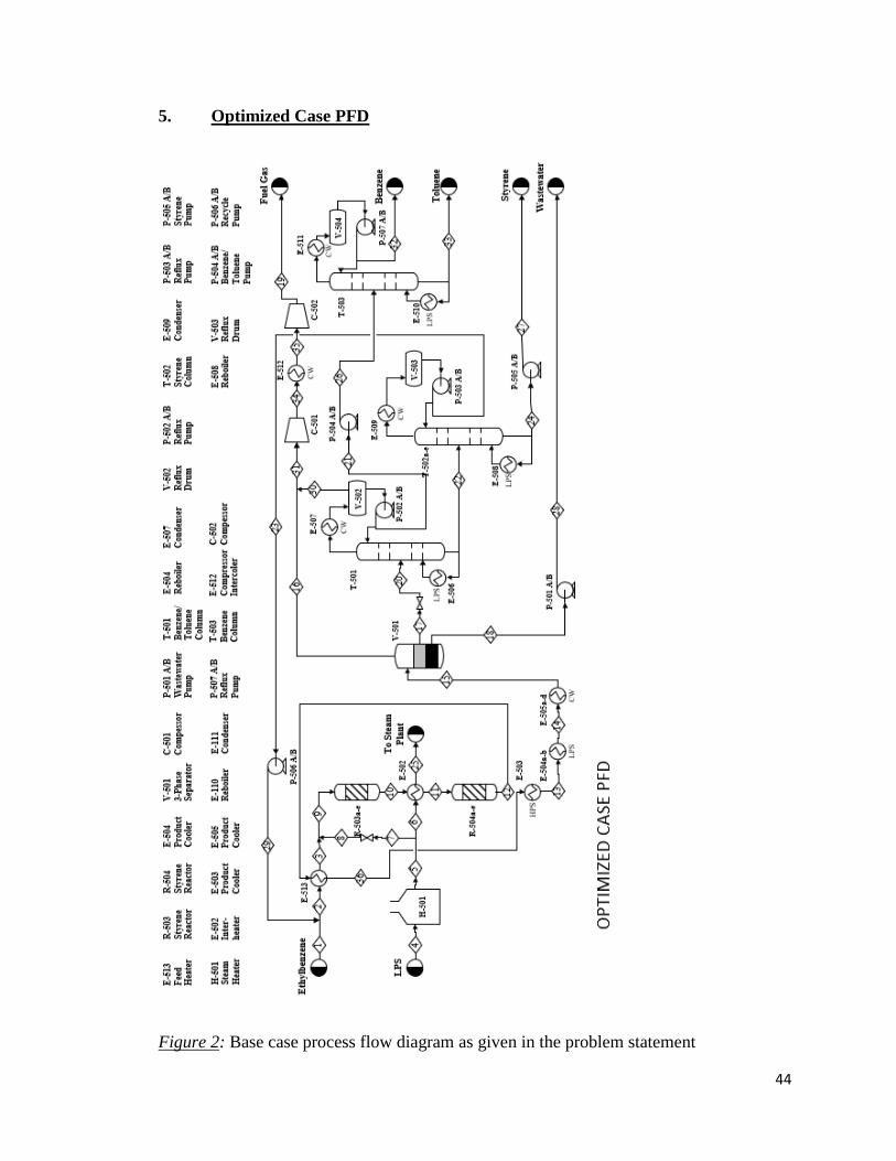
44

5. Optimized Case PFD

Figure 2: Base case process flow diagram as given in the problem statement

45

6. Optimized Case Stream Table

Table 2: Optimized case stream table as calculated for ChE 451

Stream No. 1 2 3 4 5 6 7 8 9

Temperature (°C) 136 107 225 159 800 800 800 800 525

Pressure (kPa) 203 203 188 600 565 565 565 188 188

Vapor Mole Fraction 0 0 1 1 1 1 1 1 1

Total Flow (kg/h) 19548 57071 57071 180973 180973 116368 64606 64606 121676

Total Flow (kmol/h) 185 538 538 10046 10046 6459 3586 3586 4125

Comp. Flow (kmol/h)

Water 0 0 0 10046 10046 6459 3586 3586 3586

Ethylbenzene 181 533 533 0 0 0 0 0 533

Styrene 0 1.2 1.2 0 0 0 0 0 1.2

Hydrogen 0 0 0 0 0 0 0 0 0

Benzene 1.8 1.8 1.8 0 0 0 0 0 1.8

Toluene 1.8 2.2 2.2 0 0 0 0 0 2.2

Ethylene 0 0 0 0 0 0 0 0 0

Methane 0 0 0 0 0 0 0 0 0

Stream No. 10 11 12 13 14 15 16 17 18

Temperature (°C) 483 575 539 270 180 65 65 65 65

Pressure (kPa) 164 149 113 98 83 68 68 68 68

Vapor Mole Fraction 1 1 1 1 1 0 1 0 0

Total Flow (kg/h) 121676 121676 121676 121676 121676 121676 2928 55355 63393

Total Flow (kmol/h) 4190 4190 4268 4268 4268 4268 210 539 3519

Comp. Flow (kmol/h)

Water 3586 3586 3586 3586 3586 3586 67 0 3519

Ethylbenzene 460 460 359 359 359 359 2.5 356 0

Styrene 63 63 121 121 121 121 0.6 121 0

Hydrogen 54 54 89 89 89 89 87 1.7 0

Benzene 6.1 6.1 25 25 25 25 1.1 24 0

Toluene 10 10 33 33 33 33 0.6 33 0

Ethylene 4.3 4.3 23 23 23 23 21 2.5 0

Methane 7.5 7.5 31 31 31 31 30 1.0 0

Stream No. 19 20 21 22 23 24 25 26 27

Temperature (°C) 157 65 50 120 91 123 700 50 123

Pressure (kPa) 240 60 40 60 25 55 555 200 200

Vapor Mole Fraction 1 0 0 0 0 0 1 0 0

Total Flow (kg/h) 221 55355 4791 50023 37523 12500 116368 4791 12500

Total Flow (kmol/h) 3469 539 55 474 353 120 6459 55 120

Comp. Flow (kmol/h)

Water 67 0 0 0 0 0 6459 0 0

Ethylbenzene 2.6 356 3.5 353 352 0.6 0 3.5 0.6

Styrene 0.6 121 0 121 1.2 119 0 0 119

Hydrogen 89 1.7 0 0 0 0 0 0 0

Benzene 4.7 24 21 0 0 0 0 21 0

Toluene 2.4 33 31 0 0 0 0 31 0

Ethylene 23 2.5 0 0 0 0 0 0 0

Methane 31 1.0 0 0 0 0 0 0 0

Stream No. 28 29 30 31 32 33 34 35 36

Temperature (°C) 65 91 50 63 80 136 157 63 429

Pressure (kPa) 200 203 40 40 170 190 98 98 113

Vapor Mole Fraction 0 0 1 1 0 0 1 1 1

Total Flow (kg/h) 63393 37523 541 3469 20 34 221 221 121676

Total Flow (kmol/h) 3519 353 11 221 1571 3219 3469 3469 4268

Comp. Flow (kmol/h)

Water 3519 0 0 67 0 0 67 67 3586

Ethylbenzene 0 352 0 2.6 0 3.5 3 3 359

Styrene 0 1.2 0 0.6 0 0 1 1 121

Hydrogen 0 0 1.7 89 0 0 89 89 89

Benzene 0 0 3.6 4.7 20 0.5 5 5 25

Toluene 0 0 1.8 2.4 0 30.5 2 2 33

Ethylene 0 0 2.4 23 0.1 0 23 23 23

Methane 0 0 1.0 31 0 0 31 31 31

46

7. Optimized Case Utility Summary Table

8. Optimized Case Equipment Summary Table

Utility Summary for Unit 500

bfw hps bfw lps lps bfw

18588 kg/h 9486.927 kg/h 4739512 kg/h 10366.73 kg/h

lps bfw

518690 kg/h 43652.02 kg/h 1642037 kg/h

lps bfw

53053 kg/h 1060.334 kg/h 19547.29 kg/h

E-506

E-508 E-509

E-503 E-504 E-505

cw

E-507

E-510 E-511

cw

cw

E-512

cw

cw

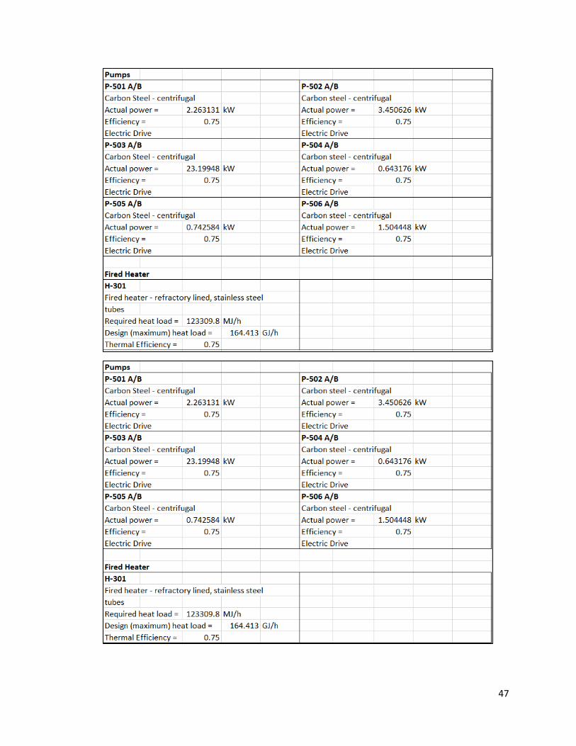
47

48

9. Optimized Case Pro/II

49

10. Optimized Case Income/Cash Flow Statement

50

11. Thermodynamic Flowsheet

51

Appendix C- Optimization Materials and Steps

1. Sensitivity Graph

Figure 3: Results from sensitivity analysis completed on the base case styrene process

2. Economic Comparison (Reactor Type)

NPV Contribution Isothermal Adiabatic Difference

Raw Materials -$1178 M -$1008 M $170 M

Utilities -$69 M -$66 M $3 M

FCI -$137 M -$190 M -$53 M

NPV -$320 M -$264 M $56 M

3. Economic Comparison (Reactor Conditions)

NPV Contribution Adiabatic

Adiabatic with Changes Difference

Raw Materials -$1008 M -$874 M $134 M

Utilities -$66 M -$74 M -$8 M

FCI -$190 M -$226 M -$36 M

NPV -$264 M -$204 M $60 M

(300)

(200)

(100)

-

100

200

300

-30% -20% -10% 0% 10% 20% 30%

Dif

fere

nce

in P

rice

fro

m B

ase

Cas

e (i

n

$M

)

Percent Variance of Price

Sensitivity Analysis

Styrene Raw Materials Labor Utilities Equipment

52

4. Conversion vs. Selectivity (Volume of R-503)

5. Conversion vs. Selectivity (Temperature of R-503)

0

0.5

1

1.5

2

2.5

3

3.5

4

4.5

5

0

0.1

0.2

0.3

0.4

0.5

0.6

0.7

0.8

0.9

1

0 50 100 150 200

Sele

ctiv

ity

Co

nve

rsio

n

Volume(m^3)

CONVERSION

SELECTIVITY

0

0.5

1

1.5

2

2.5

3

3.5

4

4.5

5

0

0.1

0.2

0.3

0.4

0.5

0.6

0.7

0.8

0.9

1

400 450 500 550 600 650 700

Sele

ctiv

ity

Co

nve

rsio

n

Temperature (°C)

CONVERSION

SELECTIVITY

53

6. Conversion vs. Selectivity (Pressure of R-503)

7. Conversion vs. Selectivity (Temperature of R-503)

0

0.5

1

1.5

2

2.5

3

3.5

4

4.5

5

0

0.1

0.2

0.3

0.4

0.5

0.6

0.7

0.8

0.9

1

100 150 200 250

Sele

ctiv

ity

Co

nve

rsio

n

Pressure (kPa)

CONVERSION

SELECTIVITY

0

0.5

1

1.5

2

2.5

3

3.5

4

4.5

5

0

0.1

0.2

0.3

0.4

0.5

0.6

0.7

0.8

0.9

1

400 450 500 550 600 650 700

Sele

ctiv

ity

Co

nve

rsio

n

Temperature (°C)

CONVERSION

SELECTIVITY

54

8. Economic Comparison (Materials of Construction)

NPV Contribution

No Material Change With Material Changes Difference

Raw Materials -$875 M -$875 M -

Utilities -$74 M -$74 M -

FCI -$226 M -$114 M $112 M

NPV -$204 M -$39 M $165 M

9. Economic Comparison (Heat Integration)

NPV Contribution Without HI With HI Difference

Utilities -$74 M -$72 M $2 M

FCI -$114 M -$114 M $0.3 M

NPV $16 M $20 M $4.1 M

10. Economic Comparison (Base Case vs. Optimized Case)

Base Case Optimized Case

NPV -$320 M $31 M

DCFROR N/A 16%

AE -$52 M $5 M

55

Appendix D- Miscellaneous Information

1. Rate Laws

where pi is the partial pressure of component i in Pa, T is the temperature in K, the

activation energy is in J/mol, and the rate is in mole/(m3 catalyst* second).

2. Notes About November 2018 Presentation Deficiencies

Our engineering team addressed several deficiencies noted by the presentation

panel in this report. First, we fixed errors in the PFDs, which included changing the

names of the adiabatic reactors to R-503 and R-504, aligning the input and output streams

on the far left and far right sides of the page, and ensuring that stream 19 remained the

fuel gas stream exiting the plant. The panel also noted that the temperature of the process

is above the flash point of each component. The finished process safety section in the

paper includes this. Lastly, the panel noted a lack of sources for why the team decided to

use stainless steel clad as the material for towers T-501 and T-502; therefore, after further

research, the team selected carbon steel as the tower material and documented the source

used in the works cited section.

We also corrected calculation errors. For the presentation, we made graphs

showing the change in selectivity and conversion as temperature and pressure changed in

56

the reactor section; however, we used the incorrect definition for selectivity. Originally,

the engineering team defined it as the yield of styrene divided by the total amount of all

side products (benzene and toluene) and by products (hydrogen, ethylene, and methane).

Now, the definition is the yield of styrene divided by only the side product total. In

addition, a calculation issue in Excel occured when the team originally added tower T-

503. The additional separation caused an increase in the raw materials cost for the total

process when solving the mass balances, which did not make sense as it should only be

separating the pre-existing stream. We corrected this by using a separate tab for the T-

503 calculation.

Lastly, the most significant deficiency noted was that our graphs and tables were

not effective. Our original tables put prices per year, one-time costs, and NPV in one

place, and we denoted the significance of each adjustment in the process with percent

changes. We corrected all tables in Appendix C so they display NPV contributions (the

panel asked us to either put all the values in terms of NPV or equivalent annual operating

costs- EAOCs.) We relocated these figures into the Appendix section to make them

accessible to the reader but also to keep them separate so that they do not become a

distraction (the panel mentioned this during the presentation.) In addition, we made the

graphs shown below for the presentation; however, the NPV values are now incorrect as

we found that w did not remove the the utility cost for the isothermal reactors once we

changed them to adiabatic. However, despite this mistake, the trends observed in the

graphs did not change and this still influenced the team’s design choices. If given more

time, the team would correct these to properly reflect the accurate NPV.

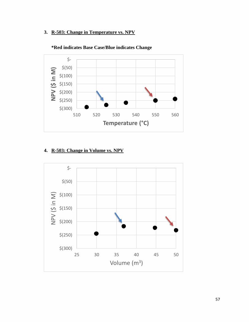
57

3. R-503: Change in Temperature vs. NPV

*Red indicates Base Case/Blue indicates Change

4. R-503: Change in Volume vs. NPV

$(300)

$(250)

$(200)

$(150)

$(100)

$(50)

$-

510 520 530 540 550 560

NP

V (

$ in

M)

Temperature (°C)

$(300)

$(250)

$(200)

$(150)

$(100)

$(50)

$-

25 30 35 40 45 50

NP

V (

$ in

M)

Volume (m3)

58

5. R-504: Change in Volume vs. NPV

$(300)

$(250)

$(200)

$(150)

$(100)

$(50)

$-

30 35 40 45 50

NP

V (

$ in

M)

Volume (m3)

59

Appendix E- Fluidized Bed Reactor Pro-II Simulation

Figure 3: Converged Pro-II flowsheet for the fluidized bed reactor in the base case

styrene process (and associated component flowrates in the product stream)

60

Table 3: Product stream from the fluidized bed reactor in the base case styrene process

(as calculated in the Excel model). When compared to the values calculated by Pro-II, the

Excel model appears to be a good approximation.

Total 4018.2 kmol/hr

Water 3467 kmol/hr

Ethylbenzene 282 kmol/hr

Styrene 95 kmol/hr

Hydrogen 66.0 kmol/hr

Benzene 26.4 kmol/hr

Toluene 30.6 kmol/hr

Ethylene 23.9 kmol/hr

Methane 27.5 kmol/hr

61

References

[1] R. Turton, R. C. Bailie, W. B. Whiting and J. A. Shaeiwitz, Analysis, Synthesis and

Design of Chemical Processes, 3rd Edition, Prentice Hall, 2009.

[2] R. Cocco, S. B. R. Karri and T. Knowlton, "Introduction to Fluidization," CEP

Magazine, November 2014.

[3] "Hydrogen Embrittlement," [Online]. Available: www.nace.org/Corrosion-

Central/Corrosion-101/Hydrogen-Embrittlement/.