Embed Size (px)
Citation preview

Optimization and Scheduling of Applications in a
Heterogeneous CPU-GPU Environment
Submitted to the School of Computer Engineering of Nanyang Technological University for
fullfillment of the Degree of Master of Engineering
by
Karan Rajendra Shetti
G1003232J
under the guidance of
Asst. Prof. Suhaib A. Fahmy
School of Computer Engineering
Jan 2014


Abstract
With the emergence of General Purpose computation on GPU (GPGPU)
and corresponding programming frameworks (OpenCL, CUDA), more applications are
being ported to use GPUs as a co-processor to achieve performance that could not be
accomplished using just the traditional processors. However, programming the GPUs
is not a trivial task and depends on the experience and knowledge of the individual
programmer. The main problem is identifying which task or job should be allocated to a
particular device. The problem is further complicated due to the dissimilar computational
power of the CPU and the GPU. Therefore, there is a genuine need to optimize the
workload balance.
This thesis presents the work done toward the author’s post graduate
study and describes the optimization of the Heterogeneous Earliest Finish Time (HEFT)
algorithm in the CPU-GPU heterogeneous environment.
In the initial chapters, different scheduling principles available are described
and an in depth analysis of three state of the art algorithms for the chosen heterogeneous
environment is presented. A comparison of fine-grained with coarse-grained scheduling
paradigms is also studied. Using state of the art StarPU scheduling framework and
exhaustive benchmarks, it is shown that the fine grained approach in much more efficient
for the CPU-GPU environment.
A novel optimization of the HEFT algorithm that takes advantage of dis-
similar execution times of the processors is proposed. By balancing the locally optimal
result with the globally optimal result, it is shown that performance can be improved sig-
nificantly without any change in the complexity of the algorithm (as compared to HEFT).
HEFT-NC (No-Cross) is compared with HEFT both in terms of speedup and schedule
length. It is shown that the HEFT-NC outperforms HEFT algorithm and is consistent
across different graph shapes and task sizes.

Acknowledgements
I would firstly likely to thank Dr. Suhaib Fahmy for giving me the oppor-
tunity to complete my Master’s program. I would like to especially thank him for his
patience and understanding while I was trying to juggle a job, coursework and the thesis.
I would also like to thank my supervisor at Airbus Innovations, Singapore,
Dr Timo Bretschneider, without whose support and encouragement, this endeavor would
have been very difficult. His constant support and push to improve my work has helped
tremendously and also his role as the devil’s advocate has improved the overall quality of
my work. I would also like to thank my colleague Asha for being my sounding board and
encouraging me to continue working by sharing her experiences of her PhD.
I would also like to thank my family for their unflinching support and belief
in me, and my housemates, Shantanu, Danny, Aiyappa and Khurana for their support
and encouragement. I truly appreciate the patience they have shown me and also re-
specting my need for a peaceful environment at home. Finally I would like to thank my
girlfriend Satvika, who in more ways than one made sure I completed this program. Her
encouragement and support has never wavered and she has helped me strive harder to
complete this study.
Karan R Shetti
Jan 2014
Nanyang Technological University, Singapore

ii

Contents
1 Introduction 3
1.1 Problem Statement . . . . . . . . . . . . . . . . . . . . . . . . . . . . . . . 5
1.1.1 Constraints . . . . . . . . . . . . . . . . . . . . . . . . . . . . . . . 6
1.2 Key Contributions . . . . . . . . . . . . . . . . . . . . . . . . . . . . . . . 6
1.3 Organization of the Report . . . . . . . . . . . . . . . . . . . . . . . . . . . 6
2 Literature Review 9
2.1 Scheduling algorithms in homogeneous architectures . . . . . . . . . . . . . 9
2.1.1 Partitioned Scheduling algorithms . . . . . . . . . . . . . . . . . . . 10
2.1.2 Global scheduling algorithms . . . . . . . . . . . . . . . . . . . . . 10
2.1.3 Heuristic based scheduling algorithms . . . . . . . . . . . . . . . . . 11
2.2 Advances in Heterogeneous architectures . . . . . . . . . . . . . . . . . . . 14
2.2.1 Heterogeneous architectures . . . . . . . . . . . . . . . . . . . . . . 14
2.3 Scheduling algorithms in heterogeneous architectures . . . . . . . . . . . . 16
2.4 Current models and frameworks for CPU-GPU environment . . . . . . . . 18
2.4.1 Harmony Model . . . . . . . . . . . . . . . . . . . . . . . . . . . . . 18
2.4.2 Predictive runtime scheduling . . . . . . . . . . . . . . . . . . . . . 19
2.4.3 Static Partitioning using OpenCL . . . . . . . . . . . . . . . . . . . 20
2.5 Summary . . . . . . . . . . . . . . . . . . . . . . . . . . . . . . . . . . . . 22
3 Programming Framework 23
3.1 Introduction . . . . . . . . . . . . . . . . . . . . . . . . . . . . . . . . . . . 23
3.2 OpenCL Application Programming Interface . . . . . . . . . . . . . . . . . 24
3.2.1 Platform Model . . . . . . . . . . . . . . . . . . . . . . . . . . . . . 24
3.2.2 Execution Model . . . . . . . . . . . . . . . . . . . . . . . . . . . . 24
3.2.3 Memory Model . . . . . . . . . . . . . . . . . . . . . . . . . . . . . 27
3.2.4 Summary . . . . . . . . . . . . . . . . . . . . . . . . . . . . . . . . 27
3.3 StarPU Scheduling Interface . . . . . . . . . . . . . . . . . . . . . . . . . . 28
3.3.1 Programming Interface [1] . . . . . . . . . . . . . . . . . . . . . . . 29
3.3.2 Task Scheduling [1] . . . . . . . . . . . . . . . . . . . . . . . . . . . 30
3.3.3 Summary . . . . . . . . . . . . . . . . . . . . . . . . . . . . . . . . 33

iv CONTENTS
4 Fine Grained Scheduling 35
4.1 Introduction . . . . . . . . . . . . . . . . . . . . . . . . . . . . . . . . . . . 35
4.2 Multi-step Applications . . . . . . . . . . . . . . . . . . . . . . . . . . . . . 36
4.2.1 Example 1 . . . . . . . . . . . . . . . . . . . . . . . . . . . . . . . . 36
4.2.2 Example 2 . . . . . . . . . . . . . . . . . . . . . . . . . . . . . . . . 36
4.2.3 Example 3 . . . . . . . . . . . . . . . . . . . . . . . . . . . . . . . . 38
4.3 Experiments and Discussion . . . . . . . . . . . . . . . . . . . . . . . . . . 39
4.4 Results and Discussion . . . . . . . . . . . . . . . . . . . . . . . . . . . . . 40
4.4.1 256 Matrix dataset . . . . . . . . . . . . . . . . . . . . . . . . . . . 40
4.4.2 1024 Matrix dataset . . . . . . . . . . . . . . . . . . . . . . . . . . 43
4.4.3 512 Matrix dataset . . . . . . . . . . . . . . . . . . . . . . . . . . . 46
4.4.4 Device Utilization . . . . . . . . . . . . . . . . . . . . . . . . . . . . 49
4.5 Summary and Conclusion . . . . . . . . . . . . . . . . . . . . . . . . . . . 51
5 HEFT-No Cross Algorithm 53
5.1 Introduction . . . . . . . . . . . . . . . . . . . . . . . . . . . . . . . . . . . 53
5.2 Problem Statement . . . . . . . . . . . . . . . . . . . . . . . . . . . . . . . 54
5.3 Algorithm Overview . . . . . . . . . . . . . . . . . . . . . . . . . . . . . . 55
5.3.1 Modification of Task Weight . . . . . . . . . . . . . . . . . . . . . . 55
5.3.2 No-Crossover Scheduling . . . . . . . . . . . . . . . . . . . . . . . . 58
5.4 Results and Discussion . . . . . . . . . . . . . . . . . . . . . . . . . . . . . 61
5.4.1 Experimental Setup . . . . . . . . . . . . . . . . . . . . . . . . . . . 61
5.4.2 Simulation Results . . . . . . . . . . . . . . . . . . . . . . . . . . . 61
5.5 Conclusion . . . . . . . . . . . . . . . . . . . . . . . . . . . . . . . . . . . . 65
5.5.1 Future Work . . . . . . . . . . . . . . . . . . . . . . . . . . . . . . . 65
6 Extension of the HEFT-NC Algorithm 67
6.1 Introduction . . . . . . . . . . . . . . . . . . . . . . . . . . . . . . . . . . . 67
6.2 Algorithm Overview . . . . . . . . . . . . . . . . . . . . . . . . . . . . . . 68
6.2.1 Modification of Task Weight . . . . . . . . . . . . . . . . . . . . . . 68
6.2.2 No-Crossover Scheduling . . . . . . . . . . . . . . . . . . . . . . . . 68
6.3 Results and Discussion . . . . . . . . . . . . . . . . . . . . . . . . . . . . . 70
6.3.1 Experimental Setup . . . . . . . . . . . . . . . . . . . . . . . . . . . 70
6.3.2 Simulation Results . . . . . . . . . . . . . . . . . . . . . . . . . . . 70
6.4 Conclusion . . . . . . . . . . . . . . . . . . . . . . . . . . . . . . . . . . . . 74
7 Conclusion and Future Work 75
7.1 Conclusion . . . . . . . . . . . . . . . . . . . . . . . . . . . . . . . . . . . . 75
7.2 Future Work . . . . . . . . . . . . . . . . . . . . . . . . . . . . . . . . . . . 77
7.2.1 Extensions to proposed algorithm . . . . . . . . . . . . . . . . . . . 77
7.2.2 Real world platform testing . . . . . . . . . . . . . . . . . . . . . . 78

CONTENTS v
Appendix A Experimental setup 79
A.1 Hardware Specification . . . . . . . . . . . . . . . . . . . . . . . . . . . . . 79
A.1.1 CPU : Intel Core 2 Duo . . . . . . . . . . . . . . . . . . . . . . . . 79
A.1.2 GPU: Nvidia Quadro 580 . . . . . . . . . . . . . . . . . . . . . . . 79
A.2 Software Specification . . . . . . . . . . . . . . . . . . . . . . . . . . . . . 80

vi CONTENTS

List of Figures
1.1 Simplistic model of HSA . . . . . . . . . . . . . . . . . . . . . . . . . . . . 4
1.2 Kaveri: Internal architecture . . . . . . . . . . . . . . . . . . . . . . . . . . 5
3.1 OpenCL platform model [2] . . . . . . . . . . . . . . . . . . . . . . . . . . 25
3.2 Work-item/Work-group example [2] . . . . . . . . . . . . . . . . . . . . . . 25
3.3 OpenCL memory model [2] . . . . . . . . . . . . . . . . . . . . . . . . . . . 27
3.4 Complete OpenCL framework [2] . . . . . . . . . . . . . . . . . . . . . . . 28
3.5 Performance model of Matrix Multiplication . . . . . . . . . . . . . . . . . 29
3.6 Execution timeline of multiple tasks . . . . . . . . . . . . . . . . . . . . . . 31
3.7 Execution model of StarPU [1] . . . . . . . . . . . . . . . . . . . . . . . . 33
4.1 Performance model for recursive Gaussian task . . . . . . . . . . . . . . . 37
4.2 Performance model for matrix transpose task . . . . . . . . . . . . . . . . . 37
4.3 Execution Time - 256 dataset . . . . . . . . . . . . . . . . . . . . . . . . . 40
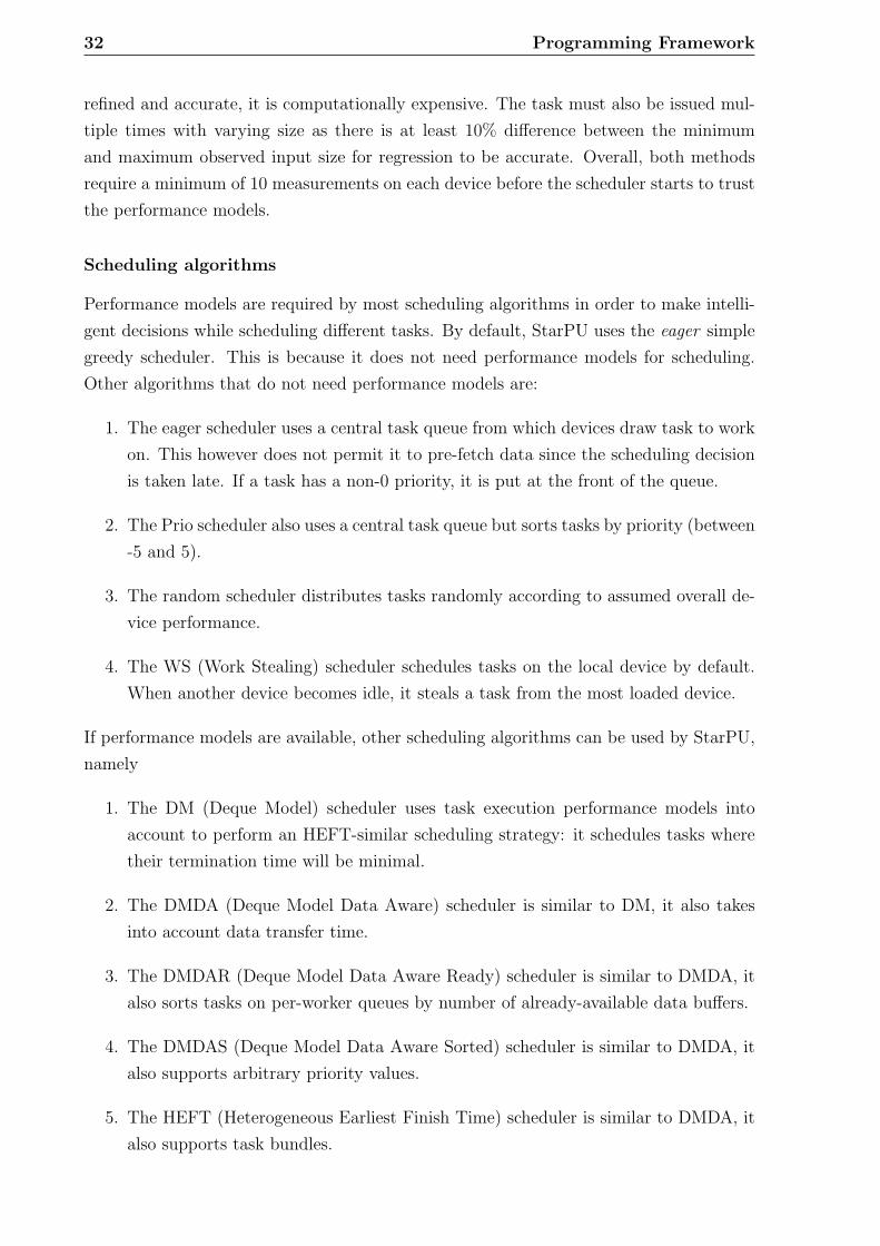
4.4 Atomic HEFT - 256 Dataset . . . . . . . . . . . . . . . . . . . . . . . . . . 41
4.5 Atomic WS - 256 Dataset . . . . . . . . . . . . . . . . . . . . . . . . . . . 41
4.6 Non Atomic HEFT - 256 Dataset . . . . . . . . . . . . . . . . . . . . . . . 42
4.7 Non Atomic WS - 256 Dataset . . . . . . . . . . . . . . . . . . . . . . . . . 42
4.8 Execution Time - 1024 dataset . . . . . . . . . . . . . . . . . . . . . . . . . 43
4.9 Atomic HEFT - 1024 dataset . . . . . . . . . . . . . . . . . . . . . . . . . 44
4.10 Atomic WS - 1024 dataset . . . . . . . . . . . . . . . . . . . . . . . . . . . 44
4.11 Non-Atomic HEFT - 1024 dataset . . . . . . . . . . . . . . . . . . . . . . . 45
4.12 Non-Atomic WS - 1024 dataset . . . . . . . . . . . . . . . . . . . . . . . . 45
4.13 Execution Time - 512 dataset . . . . . . . . . . . . . . . . . . . . . . . . . 46
4.14 Atomic HEFT - 512 Dataset . . . . . . . . . . . . . . . . . . . . . . . . . . 47
4.15 Atomic WS - 512 Dataset . . . . . . . . . . . . . . . . . . . . . . . . . . . 47
4.16 Non-Atomic HEFT - 512 dataset . . . . . . . . . . . . . . . . . . . . . . . 48
4.17 Non-Atomic WS - 512 dataset . . . . . . . . . . . . . . . . . . . . . . . . . 48
4.18 Utilization of CPU and GPU . . . . . . . . . . . . . . . . . . . . . . . . . . 50
4.19 Utilization of devices - Work Steal . . . . . . . . . . . . . . . . . . . . . . . 50
5.1 Example of random DAG . . . . . . . . . . . . . . . . . . . . . . . . . . . 57
viii LIST OF FIGURES
5.2 Application trace of HEFT . . . . . . . . . . . . . . . . . . . . . . . . . . . 60
5.3 Application trace of HEFT-NC . . . . . . . . . . . . . . . . . . . . . . . . 60
5.4 Speedup comparison α = 0.1 . . . . . . . . . . . . . . . . . . . . . . . . . . 62
5.5 Speedup comparison α = 5 . . . . . . . . . . . . . . . . . . . . . . . . . . . 62
5.6 Speedup comparison α = 10 . . . . . . . . . . . . . . . . . . . . . . . . . . 63
5.7 SLR comparison over different graph shapes . . . . . . . . . . . . . . . . . 63
5.8 SLR comparison over different CCR . . . . . . . . . . . . . . . . . . . . . . 64
6.1 Speedup comparison across different CCR, for given shape (alpha) . . . . . 71
6.2 Speedup comparison across different alpha, for given CCR . . . . . . . . . 71
6.3 SLR comparison over different graph shapes . . . . . . . . . . . . . . . . . 73
6.4 SLR comparison over different communication ratios . . . . . . . . . . . . 73

List of Tables
4.1 Execution time for mvmAtomic Task (in ms) . . . . . . . . . . . . . . . . . 36
4.2 Execution time for mulFFT Task (in ms) . . . . . . . . . . . . . . . . . . . 38
5.1 DAG Rank table . . . . . . . . . . . . . . . . . . . . . . . . . . . . . . . . 57
5.2 Definitions . . . . . . . . . . . . . . . . . . . . . . . . . . . . . . . . . . . . 59
5.3 SLR comparison over varying CCR . . . . . . . . . . . . . . . . . . . . . . 64
6.1 Definitions . . . . . . . . . . . . . . . . . . . . . . . . . . . . . . . . . . . . 69
6.2 Average SLR for 4 processors . . . . . . . . . . . . . . . . . . . . . . . . . 72
6.3 Average SLR for 8 processors . . . . . . . . . . . . . . . . . . . . . . . . . 72
A.1 CPU specification . . . . . . . . . . . . . . . . . . . . . . . . . . . . . . . . 79
A.2 CPU specification . . . . . . . . . . . . . . . . . . . . . . . . . . . . . . . . 79

2 LIST OF TABLES
Chapter 1
Introduction
The computing requirements of applications have been growing at a rapid pace. Conven-
tional single core processors are incapable of delivering the required processing power as
they are unable to overcome the three walls: Memory, Instruction level parallelism and
Power wall. Even the traditional method of increasing performance, i.e. increasing clock
frequency is not always optimal and after a point physically infeasible [3]. Multi-core
CPU and many-core GPU (Graphical Processing Unit) have been able to alleviate this
problem and have emerged as a cost effective means of scaling applications [3]. The mod-
ern GPU is a specialized hardware, which is able to execute highly parallel computations.
It focuses more on data processing rather than caching and flow control [4]. GPUs which
have traditionally been used for graphic rendering are now increasingly being used for
non-graphical applications. This has given birth to a new field of study called GPGPU
(General Purpose computation on GPU) [5] and owing to its high performance, GPUs
are increasingly being used in image processing, simulations, spectral analysis and other
scientific applications [6]. Keeping in mind these processing capabilities of GPU, sig-
nificant research has been conducted to seek ways to use the power of GPUs for general
purpose computing [7, 8, 9, 10, 11]. However, programmability of GPU still remains a
challenging task. It has become easier with the introduction of programming frameworks
like OpenGL, CUDA and OpenCL. However, all these frameworks require manual mem-
ory management and work distribution, which makes it more challenging as sub optimal
programming can severely degrade performance [8]. While GPUs have impressive com-
puting power, their specialized hardware may not be optimal for some applications, i.e.
algorithms need to be inherently parallel and involve enough data processing to overcome
memory latencies. This has led to the trend of using both CPU and GPU in a heteroge-
neous environment. This technique has been successful as most desktops and notebooks
are equipped with multi-core CPU and GPU. AMD has recently introduced new fusion
processors called APU (Accelerated Processing Units) which combine both CPU and GPU
in one chip [7, 12]. In the case of the APU, the CPU and GPU work in tandem with
shared system memory, and the key advantage here is lower power consumption when
4 Introduction
running modern applications that are designed to leverage on the advantages of both the
CPU and GPU. Applications that deal with analytics, search and facial recognition are
some aspects that stand to gain from this boost [13].
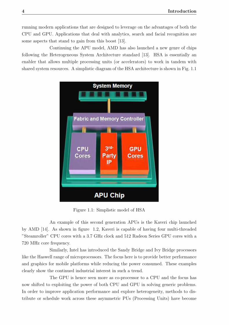
Continuing the APU model, AMD has also launched a new genre of chips
following the Heterogeneous System Architecture standard [13]. HSA is essentially an
enabler that allows multiple processing units (or accelerators) to work in tandem with
shared system resources. A simplistic diagram of the HSA architecture is shown in Fig. 1.1
Figure 1.1: Simplistic model of HSA
An example of this second generation APUs is the Kaveri chip launched
by AMD [14]. As shown in figure 1.2, Kaveri is capable of having four multi-threaded
”Steamroller” CPU cores with a 3.7 GHz clock and 512 Radeon Series GPU cores with a
720 MHz core frequency.
Similarly, Intel has introduced the Sandy Bridge and Ivy Bridge processors
like the Haswell range of microprocessors. The focus here is to provide better performance
and graphics for mobile platforms while reducing the power consumed. These examples
clearly show the continued industrial interest in such a trend.
The GPU is hence seen more as co-processor to a CPU and the focus has
now shifted to exploiting the power of both CPU and GPU in solving generic problems.
In order to improve application performance and explore heterogeneity, methods to dis-
tribute or schedule work across these asymmetric PUs (Processing Units) have become

1.1 Problem Statement 5
Figure 1.2: Kaveri: Internal architecture
more important. Conventional scheduling algorithms may not be optimal due to dissim-
ilar execution times and possibly different communication rates. The main goal of any
scheduling algorithm is to assign a task to the best suited processor such that the overall
execution time (make-span) is minimized. This problem of assigning tasks to the most
efficient processor is known to be NP-hard [15] and hence most scheduling algorithms are
based on heuristics.
1.1 Problem Statement
A platform is considered heterogeneous when dissimilar computing architectures are cou-
pled together to increase the overall computing power and solve problems faster. The
introduction of new heterogeneous architecture has led to an immense improvement in
performance at a lower cost, but also has given rise to many challenges, as the rate of
execution of tasks is different on each processor.
This property of dissimilar execution time in heterogeneous environments has reinvig-
orated research in task scheduling. Applications like image-filtering, face recognition,
gesture recognition and audio processing are multi-step processes. There are cases when
certain steps within such applications may have skewed performance on a single device.
In problems involving multi-step applications, it is crucial to determine which sections
are more efficient on a particular device.
Keeping in mind the above points, the author intends to study the problem of mapping a
set of N tasks, to a heterogeneous environment represented by a CPU and GPU such that

6 Introduction
the overall execution time of the application is minimized. As this problem has a non
polynomial solution, an approximate heuristic solution will be investigated. It is intended
to simplify this process by using predetermined information derived from static profiling
(automatic or manual).
1.1.1 Constraints
• The problem of finding a mapping for a set of tasks N to set of processing elements
is an NP hard problem. This implies only heuristic solutions can be found.
• The proposed schedule can only be non-preemptive as GPUs do not support pre-
emption.
• In order to reduce the complexity of framework, an application level as compared
to a driver level approach is used.
1.2 Key Contributions
Some of the key contributions of this thesis are:
1. A broad survey and analysis of the current literature on task scheduling in both
homogeneous and heterogeneous environments is presented. An in-depth analysis
of the more relevant literature is then discussed.
2. Using the state of the art StarPU framework, a comparison study between fine-
grained and coarse grained scheduling for the chosen environment was undertaken.
Several benchmarks were used and results are analyzed over different data sizes.
3. A novel optimization to the Heterogeneous Earliest Finish Time(HEFT) algorithm
for the CPU-GPU environment is presented. The author is able to demonstrate
significant improvements in its performance without changing the complexity of the
algorithm.
1.3 Organization of the Report
This report is organized as follows. Chapter 2 provides a comprehensive review of rele-
vant strategies used to schedule tasks both in the homogeneous and heterogeneous envi-
ronments. It also provides a critique of the strategies that can be used for a CPU-GPU
environment. Chapter 3 provides a broad overview and justification of the different
programming frameworks used in this thesis. Chapter 4 presents the results of com-
parison between a fine-grained approach and coarse-grained approach to scheduling tasks
in a CPU-GPU environment. Based on the results derived from chapter 4, chapters 5

1.3 Organization of the Report 7
6 put forward the different optimizations to the HEFT algorithm. Finally, Chapter 7
summarizes the work presented and suggest future work in the area

8 Introduction

Chapter 2
Literature Review
Parallel computing is a form of computation in which multiple operations are carried
out simultaneously [16]. It has evolved from the principle, that large problems can
often be divided into smaller ones, which are then solved in parallel [16]. Depending
on the type of hardware architecture, parallel computers can be broadly classified into
homogeneous and heterogeneous platforms [17]. Homogeneous include platforms such
as multi-core, many-core, grid computing and clusters. Here the processors are similar,
so all tasks execute with the same rate. A platform is considered heterogeneous when
dissimilar computing architectures are coupled together, for accelerating specific tasks.
Therefore, In some cases, the rate of execution of tasks is different on each processor and
in some, tasks may not be able to run on all processors. The introduction of these new
heterogeneous architectures has led to immense improvements in performance at lower
cost, but they have also given rise to many challenges. One of the interesting areas of
research has been the scheduling of tasks or programs between the specialized hardware
and the traditional processor. In Section 2.1, a brief introduction of the scheduling
algorithms available for homogeneous architectures is presented. This section describes the
different scheduling paradigms and provides insight for development in a heterogeneous
environment. In section 2.2, the advances and strategies used for high performance
computing, particularly in heterogeneous environments is presented. The latest advances
in task scheduling algorithms in CPU-GPU heterogeneous environment is elaborated in
Section 2.3. Finally in Section 2.4, a detailed account of some of the current models and
frameworks for task scheduling in CPU-GPU environment are presented
2.1 Scheduling algorithms in homogeneous architec-
tures
An application (or task set) is assumed to comprise a static set of n tasks. These tasks
give rise to a potentially infinite sequence of invocations (or jobs) [17]. Therefore task
scheduling in multi processor architecture is basically trying to solve two problems, i.e.

10 Literature Review
Allocation problems and Priority problems. Within the domain of allocation problems,
the level of task migration is used to classify different scheduling algorithms [17]
• No Migration: - Migration of tasks and jobs is not allowed as each task is allocated
to a processor.
• Task-level migration: - Jobs of one task can execute on different processors,
however each processor can execute only one job.
• Job-level migration: - A single job is allowed to migrate and execute on differ-
ent processors. This level migration gives the highest level of freedom. The only
restriction is that parallel execution of a single job is not allowed
If no migration is allowed in the scheduling algorithm, it is considered a
partitioned approach, a global approach on the other hand allows task and job migration.
2.1.1 Partitioned Scheduling algorithms
As mentioned before, in the partitioned approach, there is no support for job/task migra-
tion. This has a very important practical implication, as once the task has been scheduled
as part of a multi-processor system, it becomes a homogeneous processor problem. Well
researched algorithms [18, 19] developed for single processor scheduling can then be used.
Partition based algorithms [20, 21, 22, 23, 24] are implemented by using
one run queue for each processor. This implies that if a task overruns its worst case
performance, it only affects that processor. This localizes the problem and is more man-
ageable for large systems as compared to global scheduling. However, the disadvantages
of the partitioning approach to multiprocessor scheduling is that the determining the ideal
number of processor required by an optimal algorithm is NP-Hard [25].
2.1.2 Global scheduling algorithms
In global scheduling algorithms, tasks are permitted to migrate from one processor to
another. The focus of the majority of research done in this domain has been on job level
migration. The goal has been to optimize the preemption and scheduling of jobs [17]. In
this scheduling method, there is only one run queue for the entire system. This implies
that there will be fewer context switches as compared to the partitioned method as the
scheduler will preempt only when all processors are busy. The method is much more
efficient as any spare processing power can be used by other jobs and not just those on
the same processor.
However, the use of global scheduling algorithms was discouraged due to
the Dhall effect. Dhall and Liu [26] showed that some tasks may not be schedule-able
even though system is underutilized [4] and the tasks have low utilization. But, Philips
et. al [27] proved that augmenting a system by increasing the processor speed is more

2.1 Scheduling algorithms in homogeneous architectures 11
effective than augmenting a system by increasing the number of processors. Therefore
the Dhall effect only occurs when at least one task is needed with very high utilization
[17, 28] thereby renewing interest in global scheduling algorithms.
An example of such algorithm is P-fair scheduling [29]. In this algorithm,
all urgent tasks are scheduled first and the remaining resources are distributed to other
highest priority task contending based on the total order function [29]. This algorithm
was further improved in [30, 31], by optimizing the memory access patterns of tasks.
They propose improving throughput by discouraging tasks that generate high memory
to L2 cache traffic from being co-scheduled. This concept was further enhanced by [32]
where they consider a model to find out a group of tasks that can be encouraged to be co-
scheduled. The essence of the problem is to promote parallelism; therefore they propose a
modified P-fair algorithm which focuses on reducing the spread (the time interval in which
each job of a task is scheduled). The ideal spread would be 1, but as perfect parallelism
is not always achievable, therefore they show that cache use is more efficient when the
spread is minimized.
2.1.3 Heuristic based scheduling algorithms
1. Exact algorithms
(a) Algorithms that have a guaranteed solutions. These can also be the optimal
solutions for a given problem
2. Approximation Algorithms
(a) Algorithms that produce solutions that are guaranteed to be within a fixed
percentage of the actual optimum.
(b) Approximation algorithms are fast and have polynomial running time
3. Heuristic Algorithms
(a) These algorithms produce solutions, which are not guaranteed to be close to
the optimum
(b) The performance of heuristics is often evaluated empirically
The algorithm to map a set of tasks to a set of processing elements is NP
hard, therefore the only solution space available is the heuristic algorithms.

12 Literature Review
These can further be sub divided into:
1. Construction Heuristics [33]
(a) The algorithm begins without a known schedule, and then adds one job at a
time
(b) Dispatching rules are examples of the construction heuristics. A dispatching
rule is a rule that prioritizes all the jobs that are waiting for processing on a
machine. Whenever a machine has been freed, a dispatching rule inspects the
waiting jobs and selects the job with the highest priority
(c) Some examples of dispatching rules are [33]
i. Shortest Processing Time first (SPT)
ii. Longest Processing Time first (LPT)
iii. Earliest Completion Time first (ECT)
2. Improvement Heuristics [33]
(a) The algorithm begins with a known schedule, this is considered optimum for
solving the problem
(b) The goal is to then find a better schedule similar to the one it started with,
when adding a new task
(c) Some of the examples are: Iterative Improvement, Threshold Accepting, Sim-
ulated Annealing
Construction heuristics using dispatching rules are very useful, they are simple and fast
to implement and can find a reasonably good solution [33]. However, one of its biggest
drawbacks is unpredictability. Therefore it is more common to use composite dispatching
rules which combine multiple dispatching rules to improve the scheduling performance.
In this method, a scaling parameter can also be chosen to scale the contribution of the
dispatching rule. The most common rules are:
Min-min heuristic- For each component, the resource having the mini-
mum estimated completion time (ECT) is found. Denote this as a tuple (C, R, T), where
C is the task, R is the processor for which the minimum is achieved and T is the corre-
sponding ECT. In the next step, the minimum ECT value over all such tuples is found.
The task having the minimum ECT value is chosen to be scheduled next. This is done
iteratively until all the tasks have been mapped. The intuition behind this heuristic is
that the make span increases the least at each iterative step with the hope that the final
make-span will be as small as possible.
Max-min heuristic- The first step is exactly same as in the min-min
heuristic. In the second step the maximum ECT value over all the tuples found is chosen
and the corresponding task is mapped instead of choosing the minimum. The intuition

2.1 Scheduling algorithms in homogeneous architectures 13
behind this heuristic is that by giving preference to longer jobs, there is a hope that the
shorter jobs can be overlapped with the longer job on other processors.
Sufferage heuristic: In this heuristic, both the minimum and second best
minimum ECT values are found for each task in the first step. The difference between
these two values is defined as the sufferage value. In the second step, the task having
the maximum sufferage value is chosen to be scheduled next. The intuition behind this
heuristic is that jobs are prioritized on relative affinities. The job having a high sufferage
value suggests that if it is not assigned to the processor for which it has minimum ECT,
it may have an adverse effect on the make-span because the next best ECT value is far
from the minimum ECT value. A high sufferage value job is chosen to be scheduled next
in order to minimize the penalty of not assigning it to its best processor.

14 Literature Review
2.2 Advances in Heterogeneous architectures
Moore’s Law, which predicts that the transistor density doubles every 18 months has
continuously driven improvement in hardware architectures. However, for current ap-
plications, just increasing transistor density does not deliver the same improvement in
application performance. Various strategies are being investigated to overcome this prob-
lem [34]
• Multicore systems: Combining two or more cores on one die
– Simplest method to improve performance. By combining multiple cores, per-
formance improves while reducing power/heat consumed per core
– It may not be suitable for data intensive applications
• Specialized processors : Unconventional architectures targeting high performance in
specific applications
– Examples include vector processors, Digital Signal Processors(DSP) and Graph-
ical Processing Units (GPUs)
– While these processors are very efficient for certain applications, they are not
suitable for general purpose applications
• Heterogeneous architectures [35, 36] : Computing architectures in which conven-
tional and specialized architectures work cooperatively
– This strategy combines the benefits of the above methods wherein general
purpose computations are handled by the conventional processor and specific
applications are accelerated by the unconventional processors
– Special programming paradigms need to be applied to take full advantage of
such a system. In many cases, existing algorithms need to be redefined and
implemented
Keeping the above points in mind, it can be observed that heterogeneous
model is best suited for augmenting Moore’s Law [34].
2.2.1 Heterogeneous architectures
Programming complexity has been the main barrier toward widespread adoption of het-
erogeneous architectures. But with the rise of disruptive technologies like the multi-
core/GPU architectures, scientists have adapted and modified existing algorithms to fully
exploit it’s advantages. There are many examples of the heterogeneous environments

2.2 Advances in Heterogeneous architectures 15
CPU-FPGA Co processor Model
Highly successful model in many applications [37, 35, 36]. The main drawback of this
model is the complex programming environment(VHDL). Many C to VHDL compilers and
integrated development tools have been created to alleviate this problem. Altera, FPGA
manufacturer, has recently developed an OpenCL SDK [38] to reduce the programming
effort and time to market.
Cell Broadband Engine
Cell Broadband Engine (CELL BE) [39] was developed by through an alliance of IBM,
Toshiba and Sony. It consists of a multi core chip composed of the Parallel Processing
Element(PPE) and multiple Synergistic Processing Elements(SPE). The PPE and SPE
are connected through an internal High Speed Bus and optimized for single precision
floating point operations [39]. However, this technology has not been very successful due
to limited support available for its programming framework.
CPU-GPU Co-processor Model
GPUs have been used for general purpose computation for over a decade [5]. By increasing
parallelism instead of frequency, GPUs have been able to improve performance while
reducing power requirements. One of the drawbacks of increasing parallelism [5, 35, 36]
is that it only accelerates parallel code. Sequential execution and control logic are not very
efficient on the GPU. This serial section hence becomes the bottleneck during execution,
thus most applications are benefited by combining multi-core CPUs and massively parallel
GPUs [34]. Applications in Query co-processing [40] can especially benefit from such a
architecture. It is also observed that closely coupling the CPU and GPU allows sharing
of resources like memory and cache allowing greater acceleration of applications [40]
CPUs are designed to handle logical functions owing to large die area ded-
icated to caches and instruction level parallelism. This reduces the die are for integer
and floating point calculators. This also reduces the number of cores that placed on the
same die (typically 4-8). On the other hand, GPUs have much simpler cores and simpler
control logic [36]. In the Fermi [41] based architecture, 512 accelerator cores are available.
These cores are organized into 16 streaming multiprocessors and are clocked at roughly
1.5 GHz.
The latest GPU developed by Nvidia is the Kepler class [42]. It is divided
into 4 multiprocessors with 192 cores each totaling to 1536 cores. This class of GPUs
operates at a lower frequency of 1 GHz. The next generation 28 nm production process
coupled with lower operating frequency drastically lowers the power consumption. ling
to 1536 cores. This class of GPUs operates at a lower frequency of 1 GHz. The next
generation 28 nm production process coupled with lower operating frequency drastically
lowers the power consumption.

16 Literature Review
2.3 Scheduling algorithms in heterogeneous architec-
tures
As described in the section 2.1, scheduling algorithms for homogeneous architectures
has been well explored. While scheduling in heterogeneous architectures has also been
covered well, it has mainly been restricted to distributed and grid systems [43, 44, 45].
The research in this area for heterogeneous architectures like the GPUs within a single
machine has only picked over the last five years [46, 12, 47, 3, 48] due to improvement
in architecture technology. Due to the specialization of GPU hardware, there are more
considerations that need to be taken into account for [4], such as:
• Computing model of task, either adapted to CPU or GPU
• Amount of computing resources
• Difference in the memory architecture of the GPU
• Bottleneck of data transfers between CPU and GPU
A simple method was presented by Wang et al. [4], where tasks are divided into two
categories, computing tasks and communicating tasks. A hierarchical control data flow
is constructed where computing tasks are operating nodes and communicating tasks are
transmitting nodes. Using this task partitioning and execution runtime of tasks, the
algorithm decides which processing element the task runs on. The method proposed is
very simplistic and vague; the authors compare their solution with a traditional method
and claim about 23% improvement in performance. However details of the comparison
are not well documented.
In the method proposed by Jimenez et al. [43], a predictive user level sched-
uler is used which schedules tasks based on previous performance on a CPU and a GPU.
This algorithm is further elaborated in section 2.4.2. The Harmony framework [49] which
is analyzed in section 2.4.1 represents programs as a sequence of kernels. This framework
considers scheduling of these kernels based on the suitability of the kernels towards a
particular architecture. Using a multivariate regression model, they dynamically assign
different tasks to the processing elements. The Qilin framework [48] on the other hand
predicts run time using similar regression models offline. After extensive profiling of tasks
offline, using different input parameters, a linear model is created. This method however
may not be suitable for all applications and in some cases may require extensive profiling.
MapReduce is a programming model that enables massive data processing in large scale
computing environments. This model can take advantage of the superior performance of
GPUs. One such framework which considers task scheduling is illustrated by Shirahata
et al. [47]. The industry standard Hadoop framework [50] is used and extended to invoke
CUDA functions. The authors suggest an approach that optimizes the schedule based on

2.3 Scheduling algorithms in heterogeneous architectures 17
minimizing the elapsed time. Task profiles are collected using heartbeat messages. At 64
nodes (best configuration) this method improves performance by 1.93 times but suffers
significant overhead due to the Hadoop map task invocation.
MARS [51] is another MapReduce framework implemented using GPUs
to speed up many web applications. However, one drawback of using the MapReduce
solution on the GPU is that of memory. GPUs have comparatively lesser memory and
may not be sufficient to solve larger web based problems which have generally process
gigabytes or terabytes of data. Therefore more experiments need to be conducted to get
more quantitative results.
A dynamic approach to schedule tasks was proposed by Ravi et al. [3] for
MapReduce problems. Programs are divided into chunks which are then distributed across
the devices. This method is beneficial as it requires minimum input from users and does
not use any profiling techniques. The general idea of this algorithm is straightforward as
it uses a master-slave model to allocate new chunks once the processing elements complete
their previous work. However, one of the drawbacks of this framework is the choice of
chunk size. Their experimental results show a high variation in performance when different
sizes are chosen. Choosing the optimal size has been left for further research [3].
Grewe et al. [46] used OpenCL and Clang [52] frameworks to analyze
programs and extract static code features to partition these programs across devices.
The key contribution of this work is a machine learning based compiler that accurately
predicts the best partitioning of a task using these static code features. A two-level
predictor is used to partition the tasks. This is a fine grained approach to solve the
scheduling problem but according to the authors themselves most of the programs are
scheduled by the level one predictor. This calls to question the need for an extensive
second level predictor. Also choice of features has not been justified and any changes in
the static features will require re-training the entire model which can be quite laborious
as machine learning algorithms are computationally expensive.
However, their approach is unique, wherein task partitioning is considered
instead of scheduling between a CPU and GPU. A detailed analysis of the same is con-
ducted in section 2.4.3.

18 Literature Review
2.4 Current models and frameworks for CPU-GPU
environment
In this section, some of the current models and interesting ideas that the author finds
relevant to his study will be presented.
2.4.1 Harmony Model
The Harmony model [49] is a runtime supported programming and execution model which
is concerned with simplifying development and ensuring binary portability and scalability
across different system configurations. The model provides
• Semantics for simplifying parallelism management
• Dynamic scheduling of compute intensive kernels
• Online monitoring based optimization for heterogeneous systems
This model is divided into two sections namely programming model and execution model.
Harmony programming model
The programming model is relatively simple: it consists of compute intensive kernels
(analogous to function calls), whose execution is managed by control decisions. The
control decisions take in a set of input variables and determine the next kernel to be
executed. As kernels are encountered, there are dispatched via blocking calls. Kernel
arguments are managed by using a shared address space. These are treated as global
variables by the runtime.
Harmony execution model
During execution, an application dispatches kernels via the Harmony API which is regis-
tered by the API along with its dependence information. Kernels in the dispatch window
are then scheduled on cores for which the binaries exist. It optimizes the schedule by using
speculative kernel execution. When an application is run via the API, it first scans the
kernels in the dispatch window without blocking. This allows it to build a graph which
represents all the data dependencies between the kernels. Control decisions determine
the number of kernels that can be scanned without blocking. Non flow dependencies are
removed by variable renaming. As the kernels complete execution, the dispatch window
and schedule are updated. The harmony model shows promising results, for a matrix mul-
tiplication application it can transparently transfer it to the GPU as the size of the matrix
increases. However it does not really propose any new heuristic for task scheduling. It
relies on the control decisions specified to make a choice between different architectures.

2.4 Current models and frameworks for CPU-GPU environment 19
But on the other hand, it provides a simple model for effectively using a CPU and a
GPU. As the model is generic it can also be extended to other architectures like FPGA’s
as long as the corresponding binary is present. This makes it an ideal runtime framework
for different heterogeneous architectures.
2.4.2 Predictive runtime scheduling
In this work by Jimenez et. al [43], a novel predictive user level scheduler based on the
past performance history is presented. The authors envision a state of the art heteroge-
neous system where all processing elements are utilized by different applications (not just
scientific) and are able to adapt their behavior to improve execution time. In the model,
function level granularity is chosen; the scheduler is used as a library in the Linux OS. It
is implemented as process level scheduler. This is done as developing it as a kernel level
scheduler poses difficulties and involves a long development time. Therefore the interface
to the scheduler is a set of C++ classes. There are two steps in the algorithm namely
Processing Element (PE) selection and task selection.
Processing Element Selection
In this step, the PE on which a task should be executed is selected. This does not
mean that execution begins immediately but is a mechanism to choose which task is
best suited for a particular PE. There are two alternatives developed for this step. One
method uses the First-Free heuristic which is scheduling the tasks on the first available
PE. However this technique is not very efficient therefore a predictive algorithm based on
past performance was developed. In this method, a performance history is maintained for
all PE and task pairs by forcing the first N calls of the same function to N different PEs.
The next function call is then scheduled according best possible execution time.
Task Selection
All algorithms in this step follow the First Come First Serve heuristic. This is one of the
main drawbacks of this work as it does not consider any load balancing techniques and
may not always be optimum.
Evaluation
In order to evaluate their work, the authors have used a mix of synthetic and real bench-
marks namely matmul, ftdock, cp and sad. Even though First Free heuristic is simple,
it shows considerable improvement in some of the benchmarks. In some cases, it claims
about 60% improvement in performance. But in other cases the improvement is insignif-
icant or even degraded. This could be because some benchmarks are biased towards one

20 Literature Review
PE. There are two variations of the predictive algorithms implemented, namely history-
gpu and estimate-hist. Both the algorithms look at the performance history and create
an ’allowed-pe’ list. In the next step history-gpu schedules the task to first available
allowed-pe while estimate-hist estimates the waiting time on all PEs and schedules the
task to the PE with lowest waiting time. Both these algorithms show more consistent
and significant speedups. history-gpu performs better as the number of PE are increased
but estimate-hist manages to balance workload between CPU and GPU better.
Analysis
This model presents a simple scheduler to optimize performance on heterogeneous archi-
tectures. As it is implemented as a library, it can also be extended to other architectures.
It shows significant improvement over just using the CPU or GPU and is able to fully
utilize both the processing elements. However, because of its simple nature, there is reduc-
tion in speedup when the number of tasks that need to be scheduled is increased. Being
a user level scheduler, there is also interference from other OS level tasks. This can also
degrade performance. Another shortcoming of this method is that they haven’t explicitly
considered the data transfer time between the CPU and GPU which is significant in many
cases.
2.4.3 Static Partitioning using OpenCL
This work [46] presents a static partitioning approach to scheduling tasks/jobs to a het-
erogeneous environment like the CPU and GPU. The OpenCL environment is used to
analyze programs and extract static code features. They claim the static approach is
superior as it does not require any offline profiling and also avoids the overheads of a
dynamic run time solution. The key contribution of this paper is a machine learning
based compiler that accurately predicts the best partitioning of a task using static code
features. They have used over 47 benchmarks which are friendly towards both CPU and
GPU to validate their claim. The static code features are extracted using Clang [52].
The OpenCL code is read by Clang which builds an abstract syntax tree. This is used
to analyze the code and extract features such as number of floating point operation or
number of memory accesses. Similar features such as memory access are coalesced and a
Principal Component Analysis (PCA) is done to reduce the dimensionality of the feature
space before the results are fed into the model.
Training Data
The training data used in this work are the static code features of OpenCL programs and
their optimal partitioning. The former is the input and the latter is the output. Using
these, a model is created. Each program is run in varying partitions, namely all work on

2.4 Current models and frameworks for CPU-GPU environment 21
(CPU, GPU), (90% on CPU 10% on GPU) and so on. The partitioning with the lowest
runtime is selected as the ideal partitioning.
Predictor
All OpenCL programs can be classified into three categories, namely
1. Executed only on CPU
2. Executed only on GPU
3. Partitioned and distributed between CPU and GPU
In order to predict the correct partition, a two level hierarchical predictor is presented.
In the first level, programs belonging to category one and two are filtered and scheduled
to the corresponding devices. Therefore the features here are reduced to two using PCA.
The remaining programs are then mapped according to third predictor. Here the features
are reduced to 11 classes; class 0 represents GPU only while class 10 represents CPU only.
All other classes represent a mix of the two.
Results
In this implementation, majority of the programs are filtered out by the first level pre-
dictor, only few programs required a more fine grained approach to partitioning. All
comparisons of speedup are made with the performance of a single core system. The
proposed approach is then compared with static strategy of CPU only, GPU only and the
dynamic approach proposed by Ravi et al [3].
GPU friendly benchmarks
In these benchmarks, for obvious reasons the GPU only approach achieves the best per-
formance. The CPU only approach loses in these benchmarks. The results of the dynamic
approach [3] are good but lose out, as some of the work is performed on the CPU, this
degrades performance as compared to GPU only approach. The prediction approach pro-
posed correctly predicts for all programs and they are scheduled on the GPU thereby
achieving optimal performance.
CPU friendly benchmarks
In these benchmarks, CPU only approach achieves the best performance and a speedup of
6.12 . GPU only achieves a speedup of 1.05 for obvious reasons. The dynamic approach
also performs badly as it suffers from overheads of transferring data to the GPU when it
is actually inefficient to do so. The partitioning approach performs slightly better and is
able to achieve a speedup 4.81.

22 Literature Review
Remaining Benchmarks
In these benchmarks, the static approaches perform the worst with a speedup 4.49(CPU)
and 6.26 (GPU) as the optimal performance is achieved only when the work is distributed.
The dynamic approach shows a lot of potential here and achieves a speedup of 8. The
partitioning approach gives an even better performance and achieves a speedup of 9.31
as it does not suffer from the scheduling overheads.
Analysis
The work in this paper is very well presented. It shows that the partitioning approach
can outperform the scheduling approach. Their method of validating their claim by using
benchmarks friendly to CPU, GPU and also a mixture gives a better perspective on
their result as compared to other works [43, 49]. However this method is a fine grained
approach to solve the scheduling problem. According to the authors themselves most of
the programs are scheduled by the level one predictor. This calls to question the need
for an extensive second level predictor. Apart from that, training the model can be quite
laborious as machine learning algorithms are computationally expensive. Also choice of
features has not been justified and any changes in the static features will require retraining
the entire model.
2.5 Summary
This chapter introduced the basics of scheduling in a parallel environment. It highlighted
the need for classifications of scheduling algorithms based on the type of architectures
they support. Section 2.1 illustrated the different algorithms used on homogeneous ar-
chitectures. It introduced the two types of scheduling algorithms based on the level of
job migration allowed. Both these methods namely the Partitioned approach and Global
scheduling approach were elaborated and the benefits and problems of the two were dis-
cussed. The current state of the art in scheduling tasks in heterogeneous architectures was
introduced in section 2.3. It also highlighted the need to use different types of strategies
due to the nature of the architectures. Many algorithms and their competencies were dis-
cussed in this section. Section 2.4 then elaborated on the chosen few models/frameworks
that this author felt was relevant to his study. The pros and cons these models were also
discussed. Therefore in conclusion, while there is a wealth of literature on the subject,
there is still a search for an optimal algorithm. Many considerations like optimizing mem-
ory transfers along with task scheduling, fine grained vs. coarse granied scheduling and
optimization of device utilization can still be studied.

Chapter 3
Programming Framework
3.1 Introduction
In order to accelerate an application using a GPGPU solution, there are many program-
ming options available. The most commonly used Application Programming Interfaces
(API) are CUDA (Compute Unified Device Architecture), OpenCL [53] (Open Com-
puting Language) and DirectCompute. DirectCompute is a GPGPU API developed by
Microsoft which uses High Level Shader Language (HLSL) syntax. It is easy to use for
existing DirectX programmer but otherwise has very little support and documentation.
OpenACC is another programming standard for parallel computing devel-
oped by Cray, CAPS, Nvidia and PGI. The standard is designed to simplify parallel
programming of heterogeneous CPU/GPU systems [54]. Similar to OpenMP, sections of
C/Fortan code can be identified and accelerated using PRAGMA compiler directives and
additional functions. Unlike OpenMP, code can be started not only on the CPU, but
also on the GPU. The directives and programming model defined in the OpenACC API
document allow programmers to create high-level host + accelerator programs without
the need to explicitly initialize the accelerator, manage data or program transfers between
the host and accelerator, or initiate accelerator start-up and shutdown [54].
CUDA is a more mature framework developed by Nvidia. It has a C like
syntax making it easier to program for existing C programmers. It provides excellent
support for different GPU optimized libraries and integrates easily into existing solutions.
However, CUDA is only supported by Nvidia GPUs. This is the main drawback; it does
not even fall back to CPU if a GPU is not detected.
StarPU [55, 1] is a runtime system capable of scheduling tasks over hetero-
geneous, accelerator based machines. It is a portable system that automatically schedules
a graph of tasks onto a heterogeneous set of processors. It is a software tool aiming to al-
low programmers to exploit the computing power of the available CPUs and GPUs, while
relieving them from the need to specially adapt their programs to the target machine
and processing units. StarPU’s run-time and programming language extensions support
24 Programming Framework
a task-based programming model. Applications submit computational tasks, with CPU
and/or GPU implementations, and StarPU schedules these tasks and associated data
transfers on available CPUs and GPUs. The data that a task manipulates are auto-
matically transferred among accelerators and the main memory, so that programmers are
freed from the scheduling issues and technical details associated with these transfers. This
framework is further elucidated in Section 3.3.
3.2 OpenCL Application Programming Interface
OpenCL is an open source API developed to enable co-processors to work in tandem with
CPUs which is maintained by the Khronos group. It is supported by many companies
like ADM, Nvidia, Intel and ARM holdings. It is similar to CUDA as it also has a C like
syntax and can be integrated easily. The main advantage of OpenCL is that it supports
multiple devices. Some examples are multi-core CPUs, multi-socket CPU, GPUs and Cell
processors.
This means that a programmer can change the hardware architecture with-
out any changes to the code as OpenCL is a standard from which vendors are expected
to derive abstractions to support their devices. Therefore it can in theory support many
more devices like FPGAs and mobile hardware in the future [2]. The ability to support
a general heterogeneous environment and wide industry support has been the motivation
to choose this API for the remainder of the project.
Each OpenCL implementation (i.e. an OpenCL library from AMD, NVIDIA,
etc.) defines platforms which enable the host system to interact with OpenCL-capable
devices.The software architecture of all implementations can be described by:
• Platform Model
• Execution Model
• Memory Model
3.2.1 Platform Model
The platform model consists of a host connected to one or more OpenCL devices [2]. A
device is divided into one or more compute units. Compute units are divided into one or
more processing elements. This hierarchy is described in the Figure 3.1. Each processing
element is executes independently as it maintains its own program counter.
3.2.2 Execution Model
The execution model of the OpenCL API [53] is defined by two parts namely kernels that
execute on one or more OpenCL devices and a host program that executes on the host.

3.2 OpenCL Application Programming Interface 25
Figure 3.1: OpenCL platform model [2]
The host program defines the context for the kernels and manages their execution. When
a kernel is submitted for execution by the host, an index space is defined. The index
space supported in OpenCL 1.0 is called an NDRange. An NDRange is an N-dimensional
index space, where N is one, two or three. It is defined by an integer array of length N
specifying the extent of the index space in each dimension.
An instance of the kernel executes for each point in this index space. This
kernel instance is called a work-item and is identified by its point in the index space, which
provides a global ID for the work-item. Each work-item executes the same code but the
specific execution pathway through the code and the data operated upon can vary per
work-item. Work-items are organized into work-groups. The work-groups provide a more
coarse-grained decomposition of the index space. As shown in figure 3.2, work-groups are
assigned a unique work-group ID with the same dimensionality as the index space used
for the work-items [53]. All work items in a workgroup execute together on the same
compute unit, thereby sharing local memory. Only work items in the same work group
can be synchronized. The size of the work groups is called the local work-size of the kernel
Figure 3.2: Work-item/Work-group example [2]

26 Programming Framework
Context
The host defines a context for the execution of the kernels. The context includes the
following resources:
• Devices: The collection of OpenCL devices to be used by the host.
• Kernels: The OpenCL functions that run on OpenCL devices.
• Program Objects: The program source and executable that implement the kernels.
• Memory Objects: A set of memory objects visible to the host and the OpenCL
devices.
The context is created and manipulated by the host using functions from the OpenCL
API. The host creates a data structure called a command-queue to coordinate execution
of the kernels on the devices.
Command Queues
The host places commands into the command-queue which are then scheduled onto the
devices within the context. These include:
1. Kernel execution commands: Execute a kernel on the processing elements of a
device.
2. Memory commands: Transfer data to, from, or between memory objects, or map
and un-map memory objects from the host address space.
3. Synchronization commands: These commands constrain the order of execution. The
command-queue schedules commands for execution on a device. These execute
asynchronously between the host and the device. Commands execute relative to
each other in one of two modes:
(a) In-order Execution: Commands are launched in the order they appear in the
command queue and complete in order. This serializes the execution order of
commands in a queue.
(b) Out-of-order Execution: Commands are issued in order, but do not wait to
complete before the following commands execute. Any order constraints are
enforced by the programmer through explicit synchronization commands. Ker-
nel execution and memory commands submitted to a queue generate event
objects. These are used to control execution between commands and to coor-
dinate execution between the host and devices.
It is possible to associate multiple queues with a single context. These queues run con-
currently and independently with no explicit mechanisms within OpenCL to synchronize
between them.

3.2 OpenCL Application Programming Interface 27
3.2.3 Memory Model
Work-items executing a kernel have access to four distinct memory regions as shown in
Figure 3.3. Each region has a specific purpose. Memory objects can be accessed by all
devices only when they are defined in the same context. The different classifications are:
Figure 3.3: OpenCL memory model [2]
1. Global Memory: This memory region permits read/write access to all work-items
in all work-groups. Work-items can read from or write to any element of a memory
object.
2. Constant Memory: A region of global memory that remains constant during the
execution of a kernel. The host allocates and initializes memory objects placed into
constant memory.
3. Local Memory: A memory region local to a work-group. This memory region can
be used to allocate variables that are shared by all work-items in that work-group.
It may be implemented as dedicated regions of memory on the OpenCL device.
Alternatively, the local memory region may be mapped onto sections of the global
memory.
4. Private Memory: A region of memory private to a work-item. Variables defined in
one work-item’s private memory are not visible to another work-item.
3.2.4 Summary
As shown in Figure 3.4, the OpenCL framework consists of program code which runs on
the Host device, kernel programs which can run on all OpenCL capable devices defined

28 Programming Framework
within the same context. Work packages are enqueued by the framework to a device and
executed either in-order or out-of-order. Memory management on the other hand needs to
be done manually using the different types of memory objects mentioned above. However,
OpenCL is still an ongoing project and is gradually being embraced by many hardware
vendors and may undergo changes in the future.
Figure 3.4: Complete OpenCL framework [2]
3.3 StarPU Scheduling Interface
StarPU [55], developed by INRIA, is a runtime system capable of scheduling tasks over
heterogeneous, accelerator based machines. It is a portable system that automatically
schedules a graph of tasks onto a heterogeneous set of processors. It is a software tool
aiming to allow programmers to exploit the computing power of the available CPUs
and GPUs, while relieving them from the need to specially adapt their programs to the
target machine and processing units. Many applications like the linear algebra libraries
MAGMA [56] and PaStiX [57] use StarPU as a backend scheduler for deployment in
a heterogeneous environment. Taking into account the extensive use of StarPU in such
applications, it is an ideal choice as a scheduler for this investigation. Applications submit
computational tasks, with CPU and/or GPU implementations, and StarPU schedules
these tasks and associated data transfers on available CPUs and GPUs. The data that a
task manipulates are automatically transferred among accelerators and the main memory,
so that programmers are freed from the scheduling issues and technical details associated
with these transfers [55]. StarPU maintains the historical data of application runtimes
over different data-sizes and builds performance models for each device. It uses these
auto-tuned models along with well-known algorithms like HEFT (Heterogeneous Earliest
Finish Time), WS (Work Steal) and other variants for scheduling tasks efficiently. In most
cases, these algorithms are sufficient; however custom scheduling techniques can also be
defined.

3.3 StarPU Scheduling Interface 29
The next two sections provide an overview of the StarPU framework, it is
not intended to be an extensive tutorial but aims to provide a basic understanding of the
framework and how scheduling decisions are made.
3.3.1 Programming Interface [1]
The programming interface of StarPU can be described using the following data struc-
tures:
1. Codelets: This data structure is used to describe the computational kernels that
can be implemented on different architectures. It also defines the data buffers and
the data access rules (READ/WRITE) that are used by the kernels.
(a) Each codelet can be associated with a performance model. These models can
take into consideration execution time by the performance model as well as
power consumption. These models are built using the execution profile of the
application over at least 10 iterations. Every time the application is run, its
execution profile is saved and the model is updated using hashing techniques.
Alternatively, by specifying different parameters during the execution ,these
models can also be derived using regression based estimates and are used by
StarPU to make scheduling decisions. An example of a performance model is
shown in figure 3.5. It describes the performance on a CPU and a GPU for a
2D matrix multiplication codelet.
Figure 3.5: Performance model of Matrix Multiplication
2. Task: The task is an instantiation of a codelet. This structure is used to apply a
codelet on a data set, on the architectures for which the codelet is defined. The
StarPU GCC plug-in views tasks as Extended C functions.
(a) Tasks may have several implementations, one for each device

30 Programming Framework
(b) Tasks may have several implementations of the same device. When invoked,
StarPU can choose any of its implementations.
(c) Data handles that are used to describe the data set that each task uses. These
handles need to be registered with StarPU and are used to data management
between different devices
(d) Callback functions can be defined for each task, these are invoked after the
successful completion of the task
(e) Other additional options like task dependencies and priority levels can also be
specified using this structure
(f) The task can also be defined as synchronous or asynchronous, which means that
the task will only be executed in the order of submission. However, the process
of task submission itself is always asynchronous (non-blocking operation).
By default, task dependencies are inferred from data dependency (sequential
coherence) by StarPU. The application can however disable sequential coherency for some
data, and dependencies be expressed by hand. A task is identified by a unique 64-bit
number chosen by the application which is referred to as a tag. Task dependencies can be
enforced either by the means of callback functions or by expressing dependencies between
tags of tasks that have not been submitted yet.
3.3.2 Task Scheduling [1]
StarPU obtains performance portability by efficiently using all computing resources at
the same time. It provides a unified view of all computational units and can effectively
map tasks in a heterogeneous environment while transparently handling low level function
like data transfer automatically. Also, by comparing the relative performance of tasks on
different processing units, processing units can automatically execute the tasks they are
best suited for.
Data Management
Data that is manipulated by the different devices needs to be registered with the StarPU
scheduler through the starpu data handle() data structure. Using these data handles it
automatically manipulates all data transfers between the devices. StarPu replicates data
on all devices and by default, stores these wherever they were used. This is to ensure
minimal data transfer overhead in case they are re-used by other tasks on the same
device. When a task modifies some data, all other copies are invalidated, and only the
device which ran that task has a valid replicate of the data.

3.3 StarPU Scheduling Interface 31
Task Submission
The starpu create task() function is used to create tasks. Once the appropriate data fields
are filled, it can be submitted to the scheduler using the starpu task submit() function.
This operation can be completely asynchronous by setting the appropriate flag during
task creation. In the ideal case, all tasks should be submitted asynchronously. The
starpu wait for task() or
starpu task wait for all() functions should be used to wait for tasks to terminate. StarPU
will then be able to rework the whole schedule, overlap computation with communication
and manage accelerator local memory usage. Figure 3.6 shows an example of multiple
tasks being submitted asynchronously and scheduled using the work-steal algorithm by
StarPU across different processing elements.
Figure 3.6: Execution timeline of multiple tasks
Task scheduling algorithms
Performance modeling
Performance modeling is the key to scheduling tasks effectively on StarPU. The ap-
plication programmer needs to configure a performance model for the codelets of the
task. There are two types of models available namely STARPU HISTORY BASED and
STARPU REGRESSION BASED. STARPU HISTORY BASED measures runtime per-
formance. This assumes that for a given set of data input/output sizes, the perfor-
mance will always be about the same. This is very true for regular kernels on GPUs
for instance (< 0.1% error) and CPUs (1% error) [1]. Records of the average run-time
of previous executions on the various processing units are stored and used for estima-
tion. This method is very useful as it has lower overhead while making scheduling
decisions. However, it inherently assumes that the execution time changes based only
on size of the data. STARPU REGRESSION BASED models performance based on
run-times but further refined by regression. Performance regularity is still assumed, but
works with various data input sizes, by applying regression over observed execution times.
STARPU REGRESSION BASED uses a∗nb regression form. While this method is more
32 Programming Framework
refined and accurate, it is computationally expensive. The task must also be issued mul-
tiple times with varying size as there is at least 10% difference between the minimum
and maximum observed input size for regression to be accurate. Overall, both methods
require a minimum of 10 measurements on each device before the scheduler starts to trust
the performance models.
Scheduling algorithms
Performance models are required by most scheduling algorithms in order to make intelli-
gent decisions while scheduling different tasks. By default, StarPU uses the eager simple
greedy scheduler. This is because it does not need performance models for scheduling.
Other algorithms that do not need performance models are:
1. The eager scheduler uses a central task queue from which devices draw task to work
on. This however does not permit it to pre-fetch data since the scheduling decision
is taken late. If a task has a non-0 priority, it is put at the front of the queue.
2. The Prio scheduler also uses a central task queue but sorts tasks by priority (between
-5 and 5).
3. The random scheduler distributes tasks randomly according to assumed overall de-
vice performance.
4. The WS (Work Stealing) scheduler schedules tasks on the local device by default.
When another device becomes idle, it steals a task from the most loaded device.
If performance models are available, other scheduling algorithms can be used by StarPU,
namely
1. The DM (Deque Model) scheduler uses task execution performance models into
account to perform an HEFT-similar scheduling strategy: it schedules tasks where
their termination time will be minimal.
2. The DMDA (Deque Model Data Aware) scheduler is similar to DM, it also takes
into account data transfer time.
3. The DMDAR (Deque Model Data Aware Ready) scheduler is similar to DMDA, it
also sorts tasks on per-worker queues by number of already-available data buffers.
4. The DMDAS (Deque Model Data Aware Sorted) scheduler is similar to DMDA, it
also supports arbitrary priority values.
5. The HEFT (Heterogeneous Earliest Finish Time) scheduler is similar to DMDA, it
also supports task bundles.

3.3 StarPU Scheduling Interface 33
6. The Pheft (parallel HEFT) scheduler is similar to HEFT, it also supports parallel
tasks (still experimental).
7. The PGreedy (Garallel Greedy) scheduler is similar to Greedy, it also supports
parallel tasks (still experimental).
3.3.3 Summary
StarPU is an open source scheduler that can be used to schedule tasks in a heterogeneous
environment. It massively reduces the amount of data transfers without any application
code modification. The unique selling point of StarPU is the tight collaboration between
its high-level data management library and its portable scheduling engine. This allows
the programmer to easily design powerful scheduling policies. An overview of the StarPU
execution model is shown in Figure 3.7. StarPU unlocks the portability of performance
on complex accelerator-based platforms: it is for instance generic enough to transparently
handle heterogeneous multi-GPU setups by hiding both low-level heterogeneity and by
dispatching tasks according to the capabilities of the different units. StarPU is not limited
to multi-core machines equipped with GPUs and Cell processors. Its asynchronous event-
driven design will for instance make it straightforward to implement an OpenCL backend.
Figure 3.7: Execution model of StarPU [1]

34 Programming Framework

Chapter 4
Fine Grained Scheduling
4.1 Introduction
As mentioned in Chapter 1, introduction of heterogeneous architecture has led to an
immense improvement in performance at lower cost. While many applications can take
advantage of the superior performance, programming them efficiently is still a topic of
active research.
Applications like image-filtering, face recognition, gesture recognition and
audio processing are multi-step processes. There are cases when certain steps within such
applications may have skewed performance on a single device. In problems involving
multi-step applications, it is crucial to determine which sections are more efficient on
a particular device as it allows a fine grained approach to scheduling tasks. The focus
here is not on partitioning the tasks themselves, but determining how such a fine grained
scheduling improves overall execution time and reduces task starvation. Work Steal (WS)
and Heterogeneous Earliest Finish Time (HEFT) [58] are ideal for comparison as they
represent the different scheduling perspectives. Work Steal is a greedy algorithm that
schedules tasks as and when a processing element becomes available, it does not take into
account the historical performance on different devices.
The main idea behind Work Steal is to improve device utilization. On the
other hand HEFT [58],can use performance models and historical data to make a quicker
decision on ideal mapping of tasks onto devices while trying to reduce overall make-span.
However, it may not be a fair algorithm as it can starve some tasks in order to run them on
a better suited device leading to poor device utilization. The following sections describe
in detail the effect of fine grained scheduling across the two scheduling algorithms using
the StarPU framework. It also shows the result when executing applications over different
data sizes.

36 Fine Grained Scheduling
4.2 Multi-step Applications
Applications, especially in the image processing domain have similar base functions. For
example, several image filtering algorithms utilize the Fourier domain (and hence FFT)
for faster processing. Hence, different applications can reuse come computation kernels.
The matrix transpose kernel, for example is the same for the FFT and the Recursive
Gaussian tasks. Other tasks like 2D matrix multiplication or matrix-vector multiplication
are also used regularly as sub-tasks within a larger algorithm. Keeping this in mind, three
multi-step applications were developed and used to evaluate the fine grained approach. All
examples have two variations, one deployed as an atomic task and the other as non-atomic
tasks. The experimental setup for these tests is mentioned in Appedndix A
4.2.1 Example 1
The first example used is matrix multiplication (matMul) followed by a matrix-vector
multiplication (vectMul). Two variants of this application were created. mvmAtomic,
is a straightforward variation, where only one task is created. The OpenCL kernels for
the two sub-sections are combined and only one OpenCL execution call is made. For
the other variant, mvmSep, two tasks are created and submitted to the StarPU scheduler
asynchronously. An explicit dependency is specified such that vectMul is executed only
after matMul. Table 4.1 shows the execution time of the tasks for different data sizes.
It can be seen that the vectMul task is more efficient on the CPU even as the data size
increases; while matMul is more efficient on the GPU only when the data processed is
large. This is an ideal example that can be used to represent non-uniform performance
within a single task.
Table 4.1: Execution time for mvmAtomic Task (in ms)
Tasks 256 512 1024
matMulCPU 174 1824 54528
GPU 564 1011 5396
vectMulCPU 1 2 8
GPU 403 402 419
mvm atomicCPU 178 1436 54216
GPU 486 1025 5417
mvm sepCPU 181 1046 5442
GPU 546 1084 14980
4.2.2 Example 2
Recursive Gaussian (recGauss) filtering is another application that is used for testing the
approach. Gaussian blurring is optimal for applications that require low pass filtering

4.2 Multi-step Applications 37
or running averages. It is a widely used effect in graphics software, typically to reduce
image noise and detail. Recursive Gaussian technique is very efficient in achieving this,
especially when long filters are used. The recursive Gaussian function consists of two
kernels, namely Gaussian filtering and Matrix transpose. From the performance models
(Figures 4.1 and 4.2) generated by StarPU we can see the inherent heterogeneity in this
algorithm, wherein the recursive Gaussian kernel performs better on the GPU as the data
size increases but the transpose binary is always efficient on the CPU. Therefore this
application, GaussSep can be divided into two tasks.
106 107 108 109
0
1,000
2,000
No of Data-Points
Execution
time(m
s)
CPU GPU
Figure 4.1: Performance model for recursive Gaussian task
106 107 108 109
0
200
400
No of Data-Points
Execution
time(m
s)
CPU GPU
Figure 4.2: Performance model for matrix transpose task

38 Fine Grained Scheduling
4.2.3 Example 3
The final application developed is 2D matrix multiplication followed by 2D Fast Fourier
Transform (FFT). FFT which has a complexity of O (N logN) is used in this example
as it is an efficient way of computing the DFT of a signal which has a complexity of
O(N2). The FFT algorithm is inherently not parallel and hence more efficient on the
CPU. Matrix multiplication on the other hand operates on a relatively larger data set
and can be parallelized very easily. It is very suited to be executed on the GPU. While
this example also shows the heterogeneity within the application, it represents a different
class of applications as the penalty of running the application on a suboptimal device is
very high. Table 4.2 shows the execution time of the individual tasks when executed on
the CPU/GPU only.
Table 4.2: Execution time for mulFFT Task (in ms),
Tasks 256 512 1024
matMul cmplx CPU 288 7030 81192
GPU 671 2360 8655
fftAtomicCPU 26 139 588
GPU 616 957 2488

4.3 Experiments and Discussion 39
4.3 Experiments and Discussion
The examples developed in the section 4.2 along with other benchmarks are deployed
using the StarPU scheduler. The average result over 20 iterations of each experiment is
used for analyzing the scheduling perspective. Seven tasks are chosen as the intended
benchmarks to analyze the different approaches. All tasks are created and submitted
to the StarPU scheduler asynchronously. The execution time is measured from when
the tasks starts execution till the callback function is called by StarPU and the task is
destroyed. As StarPU manages data transfer internally, data transfer time between the
devices are included within the execution time. The different tasks (atomic) deployed are:
1. bSearch-Binary search
2. matMul-2D Floating point Matrix multiplication
3. recGauss-Recursive Gaussian
4. mvmAtomic1- 2D matrix multiplication followed by matrix-vector multiplication
5. mvmAtomic2- 2D matrix multiplication followed by matrix-vector multiplication
6. FFT - Fast Fourier Transform
7. mulFFT - 2D matrix multiplication followed by FFT
The tasks are then split into separate non-atomic tasks as mentioned below:
1. mvmAtmomic1/2: These applications are split into two tasks, namely mvmAtomic1 1
/ 2 1 and mvmAtomic1 2 / 2 2. The first corresponds to the matrix multiplication
task and the second corresponds to matrix-vector multiplication task.
2. recGauss: This application is split into two functional tasks, namely the Gaussian
function and the transpose function as explained in the previous section. However,
as we are operating in two dimensions, the tasks need to be deployed twice, resulting
in four tasks. These are recGauss1, recGauss2, recGauss3 and recGauss4.
3. mulFFT: This application is deployed as two tasks, mulFFT1 which corresponds
to the matrix multiplication operation and mulFFT2 being the 2D FFT task.

40 Fine Grained Scheduling
4.4 Results and Discussion
4.4.1 256 Matrix dataset
If we examine the execution time when the tasks are deployed both atomically and non-
atomically, we can see that there is very little difference in execution time for small data
sets. Figure 4.3 shows the execution time of all algorithms for the 256 data-set, the non-
atomic HEFT approach has the best performance with an improvement of about 25% as
compared to its atomic counterpart. As compared to HEFT (atomic), the Work Steal
algorithm shows a marginal improvement(1%). This can be attributed to the fact that for
such computations, the CPU and GPU have similar performance with CPU performing
better in some cases.
Figures 4.4 and 4.5 show an example of the execution time-line when these
tasks are deployed atomically using the HEFT and WS algorithms. In these snapshots,
we can see that the atomic HEFT algorithm schedules most of the tasks on the CPU and
the result is similar to a CPU only approach. Figures 4.6, 4.7 show the same when
the tasks are deployed non-atomically. We can observe that a better schedule in achieved
by HEFT. Work Steal algorithm has a longer make-span but better utilization. In the
case of the HEFT algorithms, the make-span of the tasks improves significantly as fine
grained approach creates a detailed performance profile of all tasks. From this profile,
HEFT schedules matMul on the GPU instead of the CPU.
Figure 4.3: Execution Time - 256 dataset
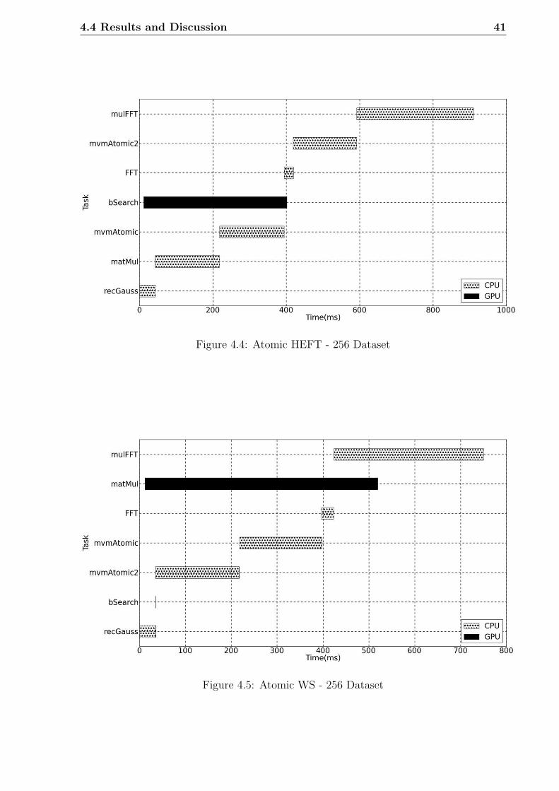
4.4 Results and Discussion 41
Figure 4.4: Atomic HEFT - 256 Dataset
Figure 4.5: Atomic WS - 256 Dataset

42 Fine Grained Scheduling
Figure 4.6: Non Atomic HEFT - 256 Dataset
Figure 4.7: Non Atomic WS - 256 Dataset
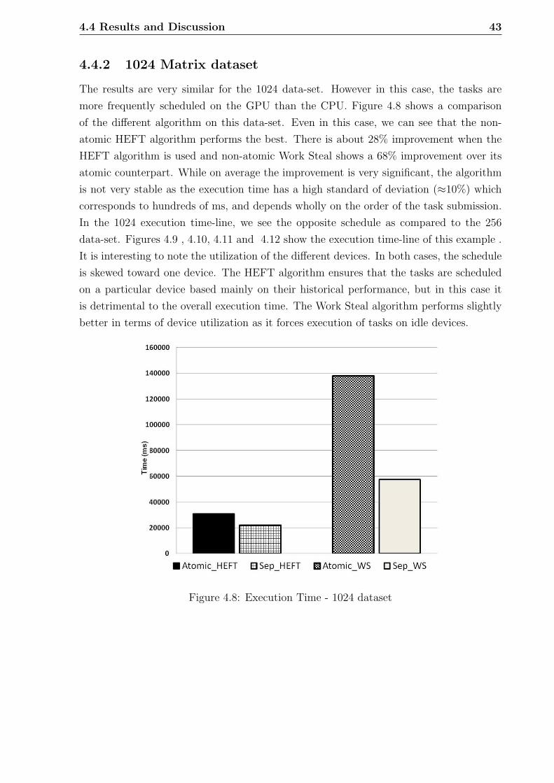
4.4 Results and Discussion 43
4.4.2 1024 Matrix dataset
The results are very similar for the 1024 data-set. However in this case, the tasks are
more frequently scheduled on the GPU than the CPU. Figure 4.8 shows a comparison
of the different algorithm on this data-set. Even in this case, we can see that the non-
atomic HEFT algorithm performs the best. There is about 28% improvement when the
HEFT algorithm is used and non-atomic Work Steal shows a 68% improvement over its
atomic counterpart. While on average the improvement is very significant, the algorithm
is not very stable as the execution time has a high standard of deviation (≈10%) which
corresponds to hundreds of ms, and depends wholly on the order of the task submission.
In the 1024 execution time-line, we see the opposite schedule as compared to the 256
data-set. Figures 4.9 , 4.10, 4.11 and 4.12 show the execution time-line of this example .
It is interesting to note the utilization of the different devices. In both cases, the schedule
is skewed toward one device. The HEFT algorithm ensures that the tasks are scheduled
on a particular device based mainly on their historical performance, but in this case it
is detrimental to the overall execution time. The Work Steal algorithm performs slightly
better in terms of device utilization as it forces execution of tasks on idle devices.
Figure 4.8: Execution Time - 1024 dataset

44 Fine Grained Scheduling
Figure 4.9: Atomic HEFT - 1024 dataset
Figure 4.10: Atomic WS - 1024 dataset

4.4 Results and Discussion 45
Figure 4.11: Non-Atomic HEFT - 1024 dataset
Figure 4.12: Non-Atomic WS - 1024 dataset

46 Fine Grained Scheduling
4.4.3 512 Matrix dataset
The results of the experiment with the 512 data-set are more interesting. Figure 4.13
shows the execution time of all approaches, there is considerable improvement in perfor-
mance when the non-atomic approach is used in both algorithms. As expected a non-
atomic HEFT solution provides the best result, it is 43% faster than its atomic equivalent.
From the time-line as shown in Figure 4.16 and 4.17, we can also observe that the devices
are utilized better.
In the Work Steal approach, we can see an improvement of 68% when
compared with its atomic counterpart. Both the CPU and GPU are utilized well. In the
non-atomic approach, tasks such as FFT, mvmAtomic1 1 and mulFFT2 are scheduled on
the GPU, which is not the optimal device for these tasks. The overall execution time is
still comparable to its HEFT counterpart. This is attributed to the fact the utilization
of the devices is quite high. From these results we can infer that improving the device
utilization is as important to reducing the overall execution time as making the correct
decision on choosing the optimum device. Therefore scheduling algorithms that can take
into account both historical run-time information and current device utilization merits
further research.
Figure 4.13: Execution Time - 512 dataset

4.4 Results and Discussion 47
Figure 4.14: Atomic HEFT - 512 Dataset
Figure 4.15: Atomic WS - 512 Dataset

48 Fine Grained Scheduling
Figure 4.16: Non-Atomic HEFT - 512 dataset
Figure 4.17: Non-Atomic WS - 512 dataset

4.4 Results and Discussion 49
4.4.4 Device Utilization
One of the aspects that plays a major role in improving the overall execution time is the
device utilization. A good schedule is able to use all devices within the heterogeneous
environment effectively. In some cases, it is more useful to schedule a task on a non-
optimal device than wait for the ideal device to be free. Figure 4.18 shows the improvement
in utilization of the CPU and GPU when the HEFT algorithm is used across 256 and 512
data sets. In the context of large data sizes such as the 1024 data set, we can see that the
GPU is utilized extensively as most tasks are efficient on it, while the CPU on the other
hand is underutilized.
For smaller data sizes, the improvement is more significant. It is observed
that the non-atomic versions are able to better utilize the devices. This is very evident
in the 512 data-set where the CPU utilization increases from 34% to 74%. In the case of
the 256 data-set the GPU utilization increases from 43% to 69%.
In the case of the Work Steal algorithm, there is a similar improvement in
performance, but no general conclusion can be derived as the results have a high variation.
Figure 4.19 depicts this variation over 10 iterations of the deploying tasks using the Work
Steal algorithm. We can observe that there is a significant fluctuation in both CPU and
GPU utilization. In this case, the task dependencies and sub-optimal scheduling lowers
the CPU utilization. Work Steal does not consider the previous performance of the task
and therefore schedules the task on the next available device. If it schedules a task on a
suboptimal device, for eg : FFT on the GPU, it takes substantially more time to complete
the task, while in the mean time the CPU waits till the dependencies are satisfied. This
leaves the CPU idle for long periods, lowering its utilization while the GPU is utilized
sub optimally.

50 Fine Grained Scheduling
Figure 4.18: Utilization of CPU and GPU
2 4 6 8 10
60
70
80
90
100
No of Iterations
Utilization
(%)
CPU GPU
Figure 4.19: Utilization of devices - Work Steal

4.5 Summary and Conclusion 51
4.5 Summary and Conclusion
In this chapter, the effectiveness of a fine grained scheduling approach in a CPU-GPU
heterogeneous environment was presented. Examples representing the different classes of
applications have been used in this study. Both inter-task (mvmAtomic, mulFFT) and
intra-task (recGauss) partitioning of applications were used to thoroughly investigate the
benefit of such an approach. The variation of the results over multiple data sets was also
studied. Using a fine grained approach provides greater freedom to the scheduler to make
decisions. This is very critical when non-homogeneous tasks are deployed as it allows
devices to be fully utilized. From the execution times and the time line graphs, we can
conclude that the non-atomic HEFT approach demonstrates the best result.
Based on the results presented in this chapter, we can conclude that map-
ping tasks to the ideal device based on only performance profile does not necessarily
improve the execution time. Other consideration that need to be taken into account are:
• Task dependencies
• Device utilization
• Memory transfer time
The effect of these factors is further studied in the next chapter.

52 Fine Grained Scheduling

Chapter 5
HEFT-No Cross Algorithm
5.1 Introduction
The main goal of any scheduling algorithm is to assign a task to the best suited processor
such that the overall execution time (make-span) is minimized. As shown in chapter 4,
performance profiles alone are not sufficient to make this decision. We must also consider
task dependencies and device utilization.
A well accepted representation of an application (set of tasks) is the Di-
rected Acyclic Graph (DAG), which characterizes the application both in terms of ex-
ecution time and inter-task dependencies. This problem of assigning tasks to the most
efficient processor is known to be NP-hard [15] and hence most scheduling algorithms
are based on heuristics. Heterogeneous Earliest-Finish-Time (HEFT) is widely accepted
algorithm that schedules a DAG onto a range of heterogeneous processors. There are two
phases within the algorithm. In the first phase, tasks are ranked and prioritized and the
second phase is used for processor selection. This algorithm has relatively low complexity
O(v2p), where v is the number of tasks and p is the number of processors. However, it
was developed before the advent of using specialized processors like GPUs [44] for general
computation.
Since then, many improvements and variations of the HEFT algorithm have been sug-
gested. Zhao and Sakellariou [59] investigated different methods to improve the ranking
function. They showed that using the average value as the task rank is not optimal. How-
ever, the results from the proposed modifications are not consistent over different graphs.
Nasri and Nafti [60] put forward another algorithm that closely mimics HEFT. Commu-
nication costs are included as part of the task rank to compensate for the heterogeneity
in communication, but the results are only marginally better than HEFT.
The PETS [61] algorithm also focuses on changing the ranking method: task ranks are
calculated not only on the Average Computation Cost (ACC) but also the Data Transmit
Cost (DTC) and Data Receive Cost (DRC). It claims to derive better schedules 71% of
the time and has lower complexity than HEFT. However, for randomly generated graphs,

54 HEFT-No Cross Algorithm
the algorithm shows marginal improvement in schedule length. Better results are ob-
tained for FFT graphs. Observing that small changes to the ranking method can affect
the performance of the scheduling algorithm, Sakellariou and Zhao [62] suggest a hybrid
method which is less sensitize toward the ranking system. The authors propose a 3-step
algorithm namely ranking, grouping and scheduling. In the grouping step, all independent
tasks are grouped together allowing greater freedom in the scheduling step to schedule
tasks in parallel. The Balanced Minimum Completion Time(BMCT) heuristic proposed
for the scheduling step outperforms HEFT for random, as well as real world work-flows
but is computationally expensive. In comparison with HEFT it is approx. seven times
slower [62].
Bittencourt et al. [63] proposed a different optimization to HEFT. The main idea here is
to minimize the Earliest Finish Time (EFT) of all the children of a node on the processor
where the selected node is to be executed. Four different variations to this look-ahead
model are presented. The algorithm performs well when the number of processors is high
but otherwise the improvement in terms of schedule length is marginal. By looking-ahead,
the complexity is also increased. Arabnejad and Barbosa [64] further optimize this ap-
proach. They put forward an algorithm that is able to look-ahead while maintaining
the same complexity as HEFT. They calculated the Optimistic Cost Table (OCT) for all
tasks and use the same for ranking and processor selection (minimize Optimistic Finish
Time instead of EFT). The algorithm also shows 4-10% improvement in make-span over
HEFT.
5.2 Problem Statement
HEFT is a well accepted list-based heuristics owing to low complexity and efficiency
[44]. Canon et. al [65] compared 20 scheduling heuristics and concluded that for random
graphs, on average, HEFT derives the best schedule. They compared these algorithms
in terms of robustness and schedule length. Computationally, the HEFT algorithm has
a complexity of O(v2p). The HEFT algorithm first assigns a priority (rank) to each task
and then uses an insertion based framework to assign tasks to a particular processor such
that the overall execution time is minimized. However, the HEFT algorithm may not be
optimal in a CPU-GPU environment as it uses average computation time to derive the
schedule and does not consider the effect of dissimilar execution times. This problem is
further exacerbated for complex task sets which have high inter task dependencies. Due
to these dependencies a single suboptimal scheduling decision can cause a significant delay
in the execution of all tasks.
Therefore, several improvements such as changing the ranking method,
looking ahead and clustering have been proposed [59, 62, 61, 66, 64, 60] over the past
few years to further improve the performance of the algorithm. In this chapter, a novel
optimization to the HEFT algorithm HEFT-NC (No Cross) is presented. The main idea

5.3 Algorithm Overview 55
behind the algorithm is balancing the globally optimal performance (Earliest Finish Time)
with the locally optimal one (computation time on different processors) by restricting the
crossing of tasks between processors. Some of the results of this study were published in
the 14’th International Conference on Parallel and Distributed Computing, Applications
and Technologies (PDCAT13) [67].
5.3 Algorithm Overview
Currently, HEFT is not fully suited to take advantage of dissimilar performance of the
CPUs and GPUs. The main idea behind the HEFT task ranking is to schedule the largest
task first, however using the average time as a metric to prioritize tasks is not optimal for
a CPU-GPU environment. The processor selection step in HEFT is based on scheduling
the highest priority task producing the lowest global Earliest Finish Time (EFT). In some
cases, we can observe that the make-span can be reduced by choosing the more optimal
processor (based on computation times) for a task rather the global EFT as later shown
in Fig. 5.3. Therefore, both the task ranking and the processor selection steps have scope
for improvement.
5.3.1 Modification of Task Weight
Approach 1
Zhao and Sakellariou [59] have experimented with various simple metrics (Median, Best
value, Worst value) to better rank tasks, but none of the metrics showed consistent per-
formance. In the author’s first approach, relative speedup was used as a metric as this is
more intuitive when comparing the performance of the CPU and GPU. The speedup is
defined as the ratio of the execution time on the slower processor to the faster processor.
This value is used to calculate the rank of the tasks. Comparing this modification with
the original HEFT (same processor selection heuristic) shows a 2.3% improvement in the
make-span averaged over 500 random DAGs. It was also observed that it produces a
better schedule 45% of the time.
Approach 2
While using the speedup as a metric shows some improvement, it does not capture all the
information about the tasks. A large speedup value does not necessarily mean that the
task is large and hence should be scheduled first. The actual time saved or the absolute
time difference of the computation times is a better metric. A similar comparison (as
Approach 1) with HEFT shows that on average, there is a 2.6% improvement in the
make-span. In this method, there is a strong bias towards tasks with large computation

56 HEFT-No Cross Algorithm
time, tasks with better speedup can be assigned lower priority. Therefore while the make
span improves, this approach produces better schedules only 38% of the time.
Approach 3
Keeping in mind the advantages and disadvantages of both the approaches, a composite
task ranking system is proposed which takes into consideration both speedup and the time
saved. By using the ratio of absolute time saved over the speedup as defined in Eq. 5.1,
we are normalizing the information across different tasks and processors.
Weightni=
abs(w(ni, pj)− w(ni, pk))
w(ni, pj)/w(ni, pk)(5.1)
Here w(ni, pj) is defined as the computation time of task ni on processor pj. This method
captures more information about the tasks and shows a 3.1% improvement in make-span
while being better than HEFT 42% of the time.
Consider the DAG shown in Fig. 5.1, the task set consists of 16 nodes with 0 being
the root node added to complete the graph. Table 5.1 shows the computation time and
the rank assigned to each task using HEFT and Approach 3. The priority of tasks as
assigned by HEFT will be {2,6,1,9,5,4,7,10,8,3,12,11,13,15,14,16} and that assigned using
the proposed approach is {2,1,6,5,9,4,8,7,3,10,11,3,12,15,14,16}. We can see that Task 1
is given higher preference compared to Task 6 even though the absolute time difference
is similar because of the higher speedup achieved. Conversely, Task 5 is given preference
over Task 9 even though their speedup is comparable as it saves a significant amount of
time. Therefore, both factors are used efficiently to determine the priority of the task.

5.3 Algorithm Overview 57
Figure 5.1: Example of random DAG
Table 5.1: DAG Rank table
Task P1 (time) P2 (time) HEFT-Rank Proposed-Rank
1 40 260 1550 355
2 286 352 1937 403
3 132 247 813 238
4 256 298 1333 262
5 97 299 1375 320
6 131 304 1617 348
7 136 104 1176 250
8 165 308 860 253
9 315 370 1399 273
10 292 213 1055 225
11 172 136 623 176
12 323 343 802 166
13 316 153 547 172
14 14 45 312 92
15 266 105 468 146
16 215 347 281 82

58 HEFT-No Cross Algorithm
5.3.2 No-Crossover Scheduling
As per the HEFT algorithm, the highest priority tasks are first scheduled on the processor
that produces the lowest finish time (globally optimal). This approach may not be the
most optimal for large and complex task sets. Sometimes, better make-span can be
achieved by scheduling tasks based on just the computation time of tasks on different
processors (locally optimal). This is more relevant for CPU-GPU environment, where the
level of heterogeneity is quite high. The formal definition of the algorithm (HEFT-NC)
is shown Algorithm 1.
Algorithm 1: HEFT-NC Algorithm
1 for all ni in N do
2 Compute modified task weight(ni)3 Compute blevel(ni)
4 end
5 StartNode←ReadyTaskList6 while ReadyTaskList is NOT NULL do
7 Select ni node in the ReadyTaskList with the maximum blevel8 for all pj in P do
9 Compute EST (ni,pj)10 EFT (ni,pj) ⇐ wi,j + EST(ni,pj)
11 end
12 Select pj with Min EFT (ni,pj)13 if wi,j <= Mink∈P (wi,k) then
14 Map node ni on processor pj which provides its least EFT15 Update T Available[pj ] and ReadyTaskList
16 else
17 Weightabstract =abs(EFT (ni ,pj )−EFT (ni ,pk ))
EFT (ni ,pj )/EFT (ni ,pk )
18
19 ifWeight(ni )
Weightabstract<= CROSS THRESHOLD then
20 Map node ni on processor pj (Cross-over)21 Update T Available[pj ] and ReadyTaskList
22 else
23 Map node ni on processor pk (No Cross-over)24 Update T Available[pk] and ReadyTaskList
25 end
26 end
27 end
The algorithm can be better understood by studying the schedules produced
as shown in Fig 5.2 and 5.3. In both cases, Task 2 is scheduled first on P1. HEFT
schedules Task 6 next followed by Task 1. In this case, Task 1 is scheduled on P2 as it
produces the lowest EFT. In comparison HEFT-NC schedules Task 1 second, ideally it
should have been scheduled on P2, however if we look at the computation time of Task 1
on P1 and P2, there is a significant difference (≈ 220 time units). So we can observe that
while globally the finish time is optimized if this task is scheduled on P2 but it is more

5.3 Algorithm Overview 59
Table 5.2: Definitions
N {n1, n2, n3, n4, n5, n6.}.Set of nodes in the DAG
P {p1,p2, p3, p4, p5, p6.}//Set of processors
wi,j Time required to execute task ni on processor pjci,j Time required to transfer data from task ni to nj
T Available[pj ] Time at which processor pj completes the execution of all thenodes previously assigned to it
EST (ni,pj) Max(T Available[pj ],Max(nm∈pred(ni )
) EFT(nm,pj)+ci,j)
EFT (ni,pj) wi,j + EST (ni,pj)
CROSS THRESHOLD Empirically defined coefficient that determines if a task shouldcrossover to a locally sub-optimal processor
efficient if we use the locally optimal processor (P1). Therefore applying the HEFT-NC
definition, the cross over to P2 is not allowed. While this can lower device utilization, it
can be observed that for large task sets the make-span is significantly improved.
The decision to cross over is critical and depends on the empirically derived value of
CROSS THRESHOLD. This value is defined as a number from 0-1. A value close to
unity will reduce the HEFT-NC schedule to the HEFT schedule. On the other hand, a
low value will not allow any cross over thereby lowering the efficiency of the heterogeneous
architecture. For this work, the value has been set to 0.3 and has shown consistent results
over 2000 DAGs as described in Section 5.4. The make-span using this method has
improved by about 4.8%. HEFT-NC also has a better schedule length ratio (SLR) of 0.98
as compared to 1.05 of HEFT. Therefore we can observe that making short term sacrifices
can significantly improve overall performance.
Lines 13-24 in the formal description of the algorithm better illustrate the
cross/no-cross decision making process. The first step is to check if processor j that pro-
duces the lowest EFT is also the most efficient processor for the task (lowest computation
time). If this case is true, (Lines 13-16) the globally optimal result matches the locally
optimal one and the task is scheduled on that processor. If these results don’t match, i.e
there exists a processor k which has a lower computation time than j, then we create an
abstract task which is an aggregate of all the previous tasks executed. This also includes
the task that needs to be scheduled. The EFT on processor p and k are used as the
computation times respectively. We create this abstract task to reduce the complexity of
the scheduling problem to a two task problem.
The composite weight as described in Eq. 5.1 is calculated for this abstract task (Line
17). Now we can compare the two tasks (abstract task and the original task to be sched-
uled) and choose the larger task. However, a simple binary comparison can overload
one processor by restricting cross-overs. Hence, a margin of error is allowed through
the CROSS THRESHOLD parameter (Lines 18-24). In the chosen example as shown
in Fig. 5.3, Tasks 1 and 2 are aggregated as a single task and their abstract weight is
calculated and compared with the weight of Task 1.

60 HEFT-No Cross Algorithm
0 200 400 600 800 1,000 1,200 1,400 1,600 1,800 2,000
26978311141615410121315
Timeline (time units)
TaskNo
P2
P1
Figure 5.2: Application trace of HEFT
0 200 400 600 800 1,000 1,200 1,400 1,600 1,800
21659831214164710111315
Timeline (time units)
TaskNo
P1
P2
Figure 5.3: Application trace of HEFT-NC

5.4 Results and Discussion 61
5.4 Results and Discussion
5.4.1 Experimental Setup
The performance of the HEFT-NC algorithm was tested exhaustively across 2000 ran-
domly generated DAGs. The following parameters were considered for generation of
these DAGs. Each of these parameters were combined in all possible combinations and
25 iterations of each combination were generated.
1. Number of tasks (N) = {10, 50, 100, 200, 500}
2. Graph shape (α) = {0.1, 1, 5, 10}
3. Computation to Communication ratio (CCR) = {0.1, 5, 10}
4. Outdegree range [0..5]
5.4.2 Simulation Results
Speedup Comparison
Figure 5.4 - 5.6 shows the speedup achieved across different parameters (α = 0.1,5,10).
We can observe that in all cases, for narrow as well as wide graphs the speedup achieved
is quite significant. The results are much better for large task sets, for smaller task
sets HEFT produces better results. This can be attributed to the fact that no-crossover
method can sometimes lengthen the schedule by overloading a processor as it assumes
that there will always be more tasks available. But as we can observe, overall, there is a
consistent improvement of about 4-6% in make-span. The best case performance of the
algorithm shows a 20% improvement.
Schedule Length Comparison
The metric most commonly used to evaluate a schedule for a single DAG is the make-span.
In order to compare DAGs with very different topologies, the metric most commonly used
is the Scheduling Length Ratio (SLR) as defined in Eq. 5.2
SLR =make− span(solution)
CPIC(5.2)
Critical Path Including Communication (CPIC) is the longest path in the DAG including
communication costs. The average SLR over different computation to communication
ratio (CCR) is shown in Table. 5.3. The improvement in performance is consistently
better than HEFT across the different CCRs. This shows that the algorithm is quite
stable.
Another important observation is the best case percentage, i.e. the amount of time

62 HEFT-No Cross Algorithm
0 50 100 200 300 400 500
−6
−4
−2
0
2
4
6
8
No of Nodes
Speedup(%
)
CCR-0.1 CCR-5 CCR-10
Figure 5.4: Speedup comparison α = 0.1
50 100 200 300 400 500
2
3
4
5
6
No of Nodes
Speedup(%
)
CCR-0.1 CCR-5 CCR-10
Figure 5.5: Speedup comparison α = 5
HEFT-NC produces shorter make-spans than HEFT. HEFT-NC is quite consistent and
on average produces better results than HEFT 68% of the time. As the task sets get bigger
and more complex, HEFT-NC produces better results. Fig. 5.7 shows the performance
of both algorithm with varying shape of the graph. For narrower graphs, there is very
little improvement in performance as compared to square or wider graphs. This is due
to the fact that dependencies curb the different permutations in which the tasks can be

5.4 Results and Discussion 63
100 200 300 400 500
2
3
4
5
No of Nodes
Speedup(%
)
CCR-0.1 CCR-5 CCR-10
Figure 5.6: Speedup comparison α = 10
scheduled.
Narrow(0.1) Square(0.5) Wide(10)2
4
6
8
10
Graph Shape
SLR
HEFT HEFT-NC
Figure 5.7: SLR comparison over different graph shapes
The performance of the algorithm over different CCR is shown in Fig. 5.8.
The improvement in performance here is significant across all ratios. The highest im-
provement can be seen in graphs with high CCR ratio because by restricting the number
of crossovers, we limit the amount of data that needs to be transferred between proces-

64 HEFT-No Cross Algorithm
Low Comm Med Comm High Comm8
8.5
9
9.5
10
CCR
SLR
HEFT HEFT-NC
Figure 5.8: SLR comparison over different CCR
sors. Therefore, even though communication costs are not taken into account explicitly,
the algorithm is indirectly benefited by using the no-crossover heuristic.
Table 5.3: SLR comparison over varying CCR
Name CCR = 0.1 CCR = 5 CCR = 10
HEFT HEFT-NC HEFT HEFT-NC HEFT HEFT-NC
Mean 12.76 12.23 11.53 10.91 12.42 11.83
Median 10.62 10.17 9.09 8.70 10.85 10.37
Std. Dev. 8.64 8.37 8.34 7.83 9.03 8.54
Best Case % 18.03 65.86 14.37 68.58 12.37 84.9

5.5 Conclusion 65
5.5 Conclusion
A novel optimization to the HEFT algorithm is presented in this chapter. The modifica-
tions proposed do not change the complexity of the algorithm but significantly improve its
performance. Modifications to both the task ranking method and the processor selection
method are suggested here.
• Task ranking: A new method to rank the tasks such that both speedup and absolute
time saved, are considered while giving priorities to the tasks. This modification
alone showed about 3-4% improvement in the make-span. While the results were
not always significant, it provided a more optimal barometer while making decisions
in the processor selection step.
• Local vs global optimization: Through exhaustive experiments it was shown that
the performance of HEFT-NC has improved significantly over the HEFT algorithm.
We have shown that in many cases, a locally optimized approach produces better
schedules. Experiments were conducted using randomly generated DAGs to test the
algorithm thoroughly.
5.5.1 Future Work
From the above results we can observe that the while HEFT-NC algorithm is very efficient,
there is still scope to improve its performance. Communication costs have not been
considered in this work. Although, indirectly it does benefit from lower memory transfers,
a better ranking system which also takes communication costs into consideration could
significantly improve performance. Another extension that incorporates multiple CPU-
GPUs can be investigated. The key challenge here would be to improve performance
without changing the complexity of the Cross/No-Cross decision.

66 HEFT-No Cross Algorithm

Chapter 6
Extension of the HEFT-NC
Algorithm
6.1 Introduction
In the previous chapter, the concept of the HEFT-No Cross algorithm is introduced.
Through exhaustive testing, it was shown that choosing the locally efficient processor as
compared to the globally efficient processor improves the overall execution time. This
approach however, was only studied in a single CPU and GPU environment.
Recent advances in GPGPU technology has led to including multiple CPU
and GPUs in the same computing framework. This industry trend toward multiple GPUs
can be observed with the advent of technologies like Unified Virtual Addressing, wherein
all devices share the same memory and GPUDirect, where communication between GPUs
can happen without host intervention. These technologies simplify the integration of
multiple GPUs within a single system.
Increasing the number of accelerators like GPUs, helps scale up performance
tremendously as it adds another level of parallelism and can also lower power requirements.
Many high end servers like the Tesla S8750 use multiple GPUs (4) along with a host
system to accelerate performance. Supercomputers like Tianhe-1A, ranked 2 in top 500
supercomputers [68] is able to generate a theoretical peak performance of 4700 petaFlops/s
using 4,096 Intel Xeon E5540 processors and 1,024 Intel Xeon E5450 processors, with 5,120
AMD GPUs. Other supercomputers like Nebulae (ranked 4) and Tsubame 2.0 (ranked
5) also use multiple GPUs. Therefore scheduling in a multi CPU-GPU environment can
be considered the next challenge in heterogeneous scheduling techniques. This chapter
describes the methods to extend HEFT-NC algorithm to a multi CPU-GPU environment.

68 Extension of the HEFT-NC Algorithm
6.2 Algorithm Overview
6.2.1 Modification of Task Weight
The weight of a task for a two processor HEFT-NC is calculated based on Eq. 5.1. The
idea there is to include information about speedup and the absolute time saved metric.
This method is straight forward for a two processor system. To extend the same idea to a
multiple CPU-GPU environment the least efficient processor for a given task is identified.
This can be considered the base processor and the respective metric can be calculated as
shown in Eq 6.1 - 6.4
MaxTimei = maxj∈p
(w(ni, pj)) (6.1)
Speedupi = MaxTimei/w(ni, pj) (6.2)
TimeDiffi = abs(MaxTimei − w(ni, pj)) (6.3)
Weightni=
SpeedupiTimeDiffi
(6.4)
Eq. 6.4 is the final equation that defines the composite weight of a given
task ni . This method, is able to combine both the speedup and time saved metric without
increasing the algorithmic complexity of the task ranking procedure. In order to support
the processor selection step, the locally optimum processor for a given task is also identified
in this step as shown in Eq. 6.5
MinProc(L)i = minj∈p
w(ni, pj) (6.5)
6.2.2 No-Crossover Scheduling
Once the task weights are generated, the tasks are ranked based on their dependencies
with other tasks. The task with highest rank is selected first in the processor selection
step. Based on the HEFT heuristic, the processor producing the lowest effective finish
time is selected and can be considered the globally optimal processor (GOP).
The computation times of a given task on GOP and the processor selected
based on Eq. 6.5 (locally optimal) are compared. If the processors have the same com-
putation time, then the task is scheduled based on the HEFT algorithm heuristics (GOP
solution). However, if the processors are different, then further analysis is carried out
to check if the task should instead be scheduled on the locally optimal processor (LOP).
This decision is similar to the decision described in Section. 5.3. By calculating the LOP
during the ranking stage using Eq. 6.5, the solution is reduced to a two processor problem

6.2 Algorithm Overview 69
and hence does not increase the complexity of the algorithm. The formal definition of the
extension of the algorithm (HEFT-NCe) is described in Algorithm 2.
Algorithm 2: HEFT-NC Extended Algorithm
1 for all ni in N do
2 Compute modified task weight(ni)3 MinProc(L)i = Minj∈p w(ni, pj)4 Compute blevel(ni)
5 end
6 StartNode←ReadyTaskList7 while ReadyTaskList is NOT NULL do
8 Select ni node in the ReadyTaskList with the maximum blevel9 for all pj in P do
10 Compute EST (ni,pj)11 EFT (ni,pj) ⇐ wi,j + EST(ni,pj)
12 end
13 Select pj with Min EFT (ni,pj)14 GlobalMinProc = j
15 if GlobalMinProc == MinProc(L)i then16 Map node ni on processor pj which provides its least EFT17 Update T Available[pj ] and ReadyTaskList
18 else
19 WeightLtask =abs(w(ni ,pglobalMin )−w(ni ,plocalMin ))
w(ni ,pglobalMin )/w(ni ,plocalMin )
20
21 Weightabstract =abs(EFT (ni ,pglobalMin )−EFT (ni ,plocalMin ))
EFT (ni ,pglobalMin )/EFT (ni ,plocalMin )
22
23 ifWeightLtaskWeightabstract
<= CROSS THRESHOLD then
24 Map node ni on processor plocalMin (Cross-over)25 Update T Available[plocalMin] and ReadyTaskList
26 else
27 Map node ni on processor pglobalMin (No Cross-over)28 Update T Available[pglobalMin] and ReadyTaskList
29 end
30 end
31 end
Table 6.1: DefinitionsN {n1, n2, n3, n4, n5, n6.}.Set of nodes in the DAG
P {p1,p2, p3, p4, p5, p6.}//Set of processors
wi,j Time required to execute task ni on processor pjci,j Time required to transfer data from task ni to nj
T Available[pj ] Time at which processor pj completes the execution of all thenodes previously assigned to it
EST (ni,pj) Max(T Available[pj ],Max(nm∈pred(ni )
) EFT(nm,pj)+ci,j)
EFT (ni,pj) wi,j + EST (ni,pj)
CROSS THRESHOLD Empirically defined coefficient that determines if a task shouldcrossover to a locally sub-optimal processor

70 Extension of the HEFT-NC Algorithm
6.3 Results and Discussion
6.3.1 Experimental Setup
The performance of the HEFT-NCe algorithm was tested exhaustively across 2000 ran-
domly generated DAGs. The following parameters were considered for generation of these
DAGs. Each of these parameters were combined in all possible combinations and 25 iter-
ations of each combination were generated.
1. Number of tasks (N) = {30, 50, 100, 200, 500, 1000 }
2. Graph shape (α) = {0.1, 5, 10}
3. Computation to Communication ratio (CCR) = {0.1, 5, 10}
6.3.2 Simulation Results
Speedup Comparison
Figures 6.1(a) and 6.1(b) show the speedup achieved for different shape parameters (α =
0.1,5,10) across all CCR ratios. We can observe that in all cases, for narrow(alpha = 0.1)
as well wide (alpha = 10) graphs the speedup achieved is quite significant. The results are
much better for large task sets. For smaller task sets HEFT produces better results which
is similar to what was observed in the two-processor solution. It can also be observed
that scaling up the number of processors does not lower the overall performance of the
algorithm which suggests that the algorithm is robust and stable. As narrow graphs do
not provide any flexibility in scheduling, HEFT has better performance in these scenarios.
Overall, HEFT-NCe show a 6% and 7% improvement in performance across all parameters
for a four and eight processor system respectively.
Considering the effects of communication between processors, Figures 6.2(a)
and 6.2(b) show the speedup achieved for a given CCR (CCR = 0.1,5,10) across different
shapes. Even in these scenarios, HEFT-NCe performs better. The improvement in per-
formance is more substantial in larger tasks sets. The effect of different communication
ratios, does not affect the performance proving that the algorithm is robust and can scale
easily over different CCRs. The best case performance in these scenarios shows a 18%
improvement while on average, a 4% improvement can be observed.

6.3 Results and Discussion 71
0 50 100 200 300 400 500
-3-2-1012345678910
No of Nodes
Speedup(%
)
Alpha-0.1 Alpha-5 Alpha-10
(a) 4 processors
100 300 500 700 1,000
012345678910
No of Nodes
Speedup(%
)
Alpha-0.1 Alpha-5 Alpha-10
(b) 8 processors
Figure 6.1: Speedup comparison across different CCR, for given shape (alpha)
0 50 100 200 300 400 500
-3-2-1012345678910
No of Nodes
Speedup(%
)
CCR-0.1 CCR-5 CCR-10
(a) 4 processors
100 300 500 700 1,000
01234567891011
No of Nodes
Speedup(%
)
CCR-0.1 CCR-5 CCR-10
(b) 8 processors
Figure 6.2: Speedup comparison across different alpha, for given CCR

72 Extension of the HEFT-NC Algorithm
Schedule Length Comparison
Comparing the SLR as defined in Eq. 5.2 of the two algorithms gives a better indication
of the utilization of the devices. Lower values indicate better utilization of the devices
during scheduling.
In the context of a 4 processor system, Table. 6.2 shows the average SLR
over all 2000 randomly generated graphs. HEFT-NCe has a lower SLR (≈ 8%) than
HEFT. It is also more stable with a lower standard deviation (≈ 11%).
The same trend is observed in an eight processor system. Table. 6.3 sum-
marizes all the results. Another important observation is the best case percentage, while
the value is lower than that observed in a two processor system (68%), HEFT-NCe is
quite consistent and on average produces better results than HEFT 55% of the time.
Table 6.2: Average SLR for 4 processors
Name HEFT HEFT-NC
Mean 2.6 2.39
Median 2.17 2.01
Std. Dev. 1.58 1.40
Best Case % 10.64 61.04
Table 6.3: Average SLR for 8 processors
Name HEFT HEFT-NC
Mean 1.46 1.34
Median 1.29 1.19
Std. Dev. 0.62 0.54
Best Case % 8.64 50.37
Further analysis of the SLR over different graph shapes and communica-
tion ratios is described through Figures 6.3(a), 6.3(b), 6.4(a) and 6.4(b). Fig. 6.3(a)
and 6.3(b) show the performance of the algorithm over varying shape of the graphs.
The performance of HEFT-NCe improves as the graphs shape increases. The best perfor-
mance improvement is seen in wide graphs owing to the flexibility available in scheduling.
Similarly, 6.4(a) and 6.4(b) show the SLR over different communication rates. It is
interesting to note that for lower communication ratio graphs, the improvement is more
significant, ≈ 9% for a 4 processor system and ≈ 14% for an eight processor system. In
this scenario, it is actually the HEFT algorithm that performs poorly
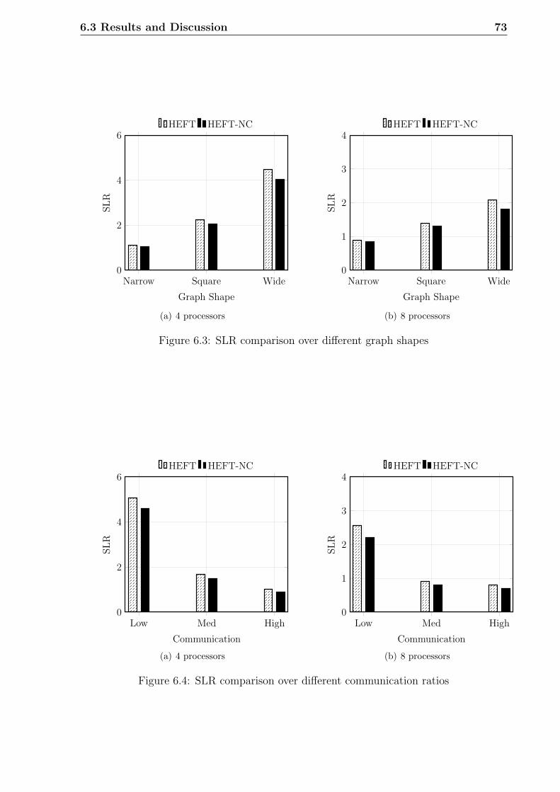
6.3 Results and Discussion 73
Narrow Square Wide0
2
4
6
Graph Shape
SLR
HEFT HEFT-NC
(a) 4 processors
Narrow Square Wide0
1
2
3
4
Graph Shape
SLR
HEFT HEFT-NC
(b) 8 processors
Figure 6.3: SLR comparison over different graph shapes
Low Med High0
2
4
6
Communication
SLR
HEFT HEFT-NC
(a) 4 processors
Low Med High0
1
2
3
4
Communication
SLR
HEFT HEFT-NC
(b) 8 processors
Figure 6.4: SLR comparison over different communication ratios

74 Extension of the HEFT-NC Algorithm
6.4 Conclusion
In this chapter, the HEFT-NC algorithm was extended to support a multi CPU-GPU
environment. The original HEFT-NC algorithm was modified both in the task ranking
and processor selection phase. The motivation behind the modifications was to ensure the
complexity of the algorithm does not increase. Through exhaustive testing, the author
has shown that the HEFT-NC algorithm is robust, stable and outperforms HEFT even
with an increase in the number of processing elements. The average SLR over different
graphs is significantly lower than HEFT which showcases the efficiency of the scheduling
principle.

Chapter 7
Conclusion and Future Work
7.1 Conclusion
With the rapid rise in computational requirements, heterogeneous architectures are being
considered as a viable solution. In this thesis, the author first introduced the problem
of scheduling in the heterogeneous environment. Some of the key contributions from the
author were highlighted and the constraints and limitations were justified.
A substantial literature review was conducted which showed the trends in
scheduling algorithms both in the homogeneous and heterogeneous environments. It can
be observed that solutions developed for conventional systems may not be applicable to
heterogeneous environments due to nature of the hardware architectures. By reviewing
the latest advances in these architectures a better understanding of the architecture was
established.
This study also investigated the state of the art scheduling algorithms for
heterogeneous environments. The various models were studied and the advantages and
disadvantages were presented. This study helped the author understand the various prob-
lems in scheduling and motivated him to focus his study by targeting
• Coarse grained vs Fine Grained scheduling
• Effect of dependencies
• Optimizing device utilization
In Chapter 4, the author studied the effect of fine grained and coarse grained
approaches to scheduling. These methodologies were compared using the StarPU envi-
ronment and several CPU friendly and GPU friendly benchmarks. Work Steal which is a
simple greedy algorithm and HEFT algorithm were used as the candidate algorithms for
the comparison.
It was observed that fine grained scheduling provided more freedom to the
chosen scheduling algorithms thereby deriving better schedules using both algorithms.
76 Conclusion and Future Work
Using the atomic (fine grain) approach improved the make-span on average by 28% across
all data sets. The fine grained approach also ensured high device utilization when using
the HEFT algorithm, but showed inconsistent results in the Work steal method due to
its greedy nature.
However, one of the drawbacks of using the fine grained approach is addi-
tional dependencies that are incurred by breaking up a complex task into simpler task.
These dependencies can severely degrade performance if the tasks are scheduled on a sub
optimal processor.
Based on these results, the author was able to propose a novel optimization
to the HEFT algorithm as described in Chapter 5. HEFT algorithm is a well established
as it produces schedules with short make-span and has low algorithmic complexity. The
author was able further improve its performance by optimizing both the task ranking
stage and processor selection stage of the algorithm without changing the complexity of
the algorithm.
In the task ranking stage, the author developed a new method to prioritize
tasks. This method takes into consideration the speedup and absolute time saved as
compared to just the average execution time in HEFT. This optimization hence is more
suited to the CPU-GPU environment as these architectures can have vastly dissimilar
execution times for a given task. Changing this method alone improved performance over
HEFT algorithm by 3-4% and produced shorter schedules.
The main contribution in this chapter is the idea that due to the vastly
different architectures, a locally optimized approach produces better results than a glob-
ally optimized approach. The HEFT-No Cross algorithm compares both these solutions
during the processor selection phase and chooses the optimal processor using a local bias.
Extensive tests were conducted using simulated data, over 2500 DAGs of
different sizes and shapes were generated. In terms of make-span, the HEFT-NC algorithm
shows a 4-6% improvement on average and a best case of 20% as compared to HEFT. The
algorithm was compared using the Schedule Length Ratio metric also and showed better
performance across all DAGs. On average, HEFT-NC produced better schedules 70% of
the time, while HEFT achieved 14% (Both achieved same results otherwise).
HEFT-NC algorithm was further extended to multi CPU - multi GPU en-
vironment to test the scalability of the algorithm. This is presented in Chapter 6. Even
in these scenarios, the HEFT-NCe algorithm outperformed HEFT by 6-8% in terms of
make-span. It produced better results 55% of the time as compared to 8% by HEFT.

7.2 Future Work 77
7.2 Future Work
With the rapid development of the technology in the semiconductor industry, it is now
possible to couple CPUs and GPUs even more closely. Both AMD and Nvidia are actively
developing platforms that are closely coupled. These hardware vendors are also trying to
reduce the effort required by programmers to benefit from GPU co-processor model, for
Eg. the ’Fusion System Architecture’ (FSA), which is a task-based queuing model is still
being developed by AMD and will be implemented in the future.
Studying the current literature in this topic, we can observe that a large
number of applications benefit from the heterogeneous environment and hence schedulers
that can exploit benefit of the CPU-GPU environment will play a critical role in the
future. As mentioned in Chapter 5 and 6, the HEFT-NC algorithm is quite robust
and scalable. It performs well for narrow as well as wide graphs, however there are still
multiple avenues in which the current work can further extended.
7.2.1 Extensions to proposed algorithm
• Communication costs PETS [61] algorithm shows that performance of HEFT can
be improved by considering both data in and data out costs. These haven’t been
taken into consideration in HEFT-NC algorithm during task ranking or the pro-
cessor selection stage. They are added during the graph traversal linearly. One
way to improve the performance could be to consider data transfer time while mak-
ing the Cross/No-Cross decision. By comparing the communication costs with the
processing time, a better decision can be made.
• Extended task profiling As mentioned in chapter 2, Grewe et al [46] propose a static
partitioning approach to schedule tasks in CPU-GPU environment. They profile the
code to determine the best architecture to run on, by extracting static code features
and classifying them. This approach could be used in the proposed approach to
further enhance the task profiles (based on execution time only). By including more
information about the actual complexity of the task, the cross/ no cross decision
can be further refined.
• Look ahead variation In many cases, especially when inter task dependencies are
high, the decision not to cross can lower processor utilization. One way to avoid
this is develop a look ahead variant, wherein the child of a particular node is also
considered. This might change the complexity of the algorithm, but as shown by
Arabnejad and Barbosa [64] this situation can be avoided by gathering the infor-
mation during the task ranking stage.

78 Conclusion and Future Work
7.2.2 Real world platform testing
The second aspect that can further examined is the integration of the proposed scheduling
algorithm in real world systems. The best approach forward would be to integrate the
scheduling algorithms within the Operating Systems(OS). GPUs can then be used as
a co-processor and applications can be seamlessly deployed on them. Fusion System
Architecture is AMD’s attempt to better utilize both the processors.
However, currently, one of the main drawbacks of GPUs is the inability to
pre-empt tasks during execution. This severely limits the type of real world systems it
can be used with. One of the ways to overcome this would be to reserve a certain number
of cores for high priority tasks, but this could lead to wastage of resources.
Therefore, completing integrating heterogeneous schedulers in the OS will
require considerable effort from both hardware vendors and OS programmers, a simpler
way to approach this problem could be by using already developed run-time schedulers
like StarPU. StarPU allows programmers to design their own scheduling policy using their
API. This can help test the algorithms developed in real-world platform and fine tune
as necessary. Implementing and testing the proposed algorithm on such platforms could
further enhance this study.
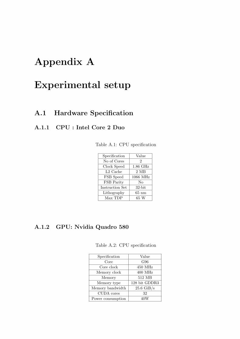
Appendix A
Experimental setup
A.1 Hardware Specification
A.1.1 CPU : Intel Core 2 Duo
Table A.1: CPU specification
Specification Value
No of Cores 2
Clock Speed 1.86 GHz
L2 Cache 2 MB
FSB Speed 1066 MHz
FSB Parity No
Instruction Set 32-bit
Lithography 65 nm
Max TDP 65 W
A.1.2 GPU: Nvidia Quadro 580
Table A.2: CPU specification
Specification Value
Core G96
Core clock 450 MHz
Memory clock 400 MHz
Memory 512 MB
Memory type 128 bit GDDR3
Memory bandwidth 25.6 GiB/s
CUDA cores 32
Power consumption 40W

80 Experimental setup
A.2 Software Specification
The following software was used during the testing:
1. Operating System-Linux Ubuntu 11.04
2. Development tools
(a) Scheduler: StarPU runtime 1.0.4
(b) Trace tool: ViTE 1.1 (Visual Trace Explorer)
(c) IDE: Eclipse Galileo

References
[1] Cedric Augonnet, Samuel Thibault, and Raymond Namyst, “StarPU: a Runtime
System for Scheduling Tasks over Accelerator-Based Multicore Machines,” Technical
Report 7240, INRIA, Mar. 2010.
[2] Benedict Gaster, Lee Howes, David R Kaeli, Perhaad Mistry, and Dana Schaa, Het-
erogeneous Computing with OpenCL: Revised OpenCL 1.0, Morgan Kaufmann, 2012.
[3] Vignesh T. Ravi, Wenjing Ma, David Chiu, and Gagan Agrawal, “Compiler and
runtime support for enabling generalized reduction computations on heterogeneous
parallel configurations,” in Proceedings of the 24th ACM International Conference
on Supercomputing. 2010, ICS ’10, pp. 137–146, ACM.
[4] Lei Wang, Yong-Zhong Huang, Xin Chen, and Chun yan Zhang, “Task scheduling of
parallel processing in CPU-GPU collaborative environment,” in Computer Science
and Information Technology, 2008, pp. 228–232.
[5] M. Harris, “General purpose computing on GPUs,” http://gpgpu.org/, 2002.
[6] Ian Buck, “Taking the plunge into GPU computing,” in GPU Gems 2, Matt Pharr,
Ed., pp. 509–519. Addison-Wesley, 2005.
[7] AMD, “AMD Technologies:Leading the Next Era of Vivid Digital Experiences,”
www.amd.com/us/products/technologies/Pages/technologies.aspx, 2011.
[8] C. Ranger, R. Raghuraman, A. Penmetsa, G. Bradski, and C. Kozyrakis, “Evalu-
ating mapreduce for multi-core and multiprocessor systems,” in High Performance
Computer Architecture, 2007, 2007, pp. 13–24.
[9] Chris J. Thompson, Sahngyun Hahn, and Mark Oskin, “Using modern graphics
architectures for general-purpose computing: a framework and analysis,” in Proceed-
ings of the 35th annual ACM/IEEE international symposium on Microarchitecture.
2002, MICRO 35, pp. 306–317, IEEE Computer Society Press.
[10] H. J. Siegel, J. K. Antonio, R. C. Metzger, M. Tan, and Y. A. Li, Parallel and
distributed computing handbook, chapter Heterogeneous computing, McGraw-Hill,
Inc., New York, NY, USA, 1996.

82 REFERENCES
[11] Shuhao Zhang, Jiong He, Bingsheng He, and Mian Lu, “Omnidb: Towards portable
and efficient query processing on parallel CPU/GPU architectures,” Proceedings of
the VLDB Endowment, vol. 6, no. 12, pp. 1374–1377, 2013.
[12] N.Brookwood, “AMD Fusion Family of APUs: Enabling a Superior, Immersive PC
Experience,”
http://sites.amd.com/us/Documents/48423B fusion whitepaper WEB.pdf, 2010.
[13] AMD, “Heterogeneous system architecture: A technical review,” http://amd-dev.
wpengine.netdna-cdn.com/wordpress/media/2012/10/hsa10.pdf, 2012.
[14] AMD, “Amd introduces kaveri, its most powerful apu ever,” http://www.pcmag.
com/article2/0,2817,2427114,00.asp, 2014.
[15] C. Boeres, J.V. Filho, and V. E F Rebello, “A cluster-based strategy for scheduling
task on heterogeneous processors,” in 16th Symposium on Computer Architecture
and High Performance Computing, SBAC-PAD. IEEE, 2004, pp. 214–221.
[16] G. S. Almasi and A. Gottlieb, Highly Parallel Computing, Benjamin-Cummings
Publishing Co., Inc., Redwood City, CA, USA, 1989.
[17] Robert I. Davis and Alan Burns, “A survey of hard real-time scheduling for multi-
processor systems,” ACM Comput. Surv., vol. 43, no. 4, pp. 1–44, Oct. 2011.
[18] Joseph Y-T Leung and Jennifer Whitehead, “On the complexity of fixed-priority
scheduling of periodic, real-time tasks,” Performance evaluation, vol. 2, no. 4, pp.
237–250, 1982.
[19] Chung Laung Liu and James W Layland, “Scheduling algorithms for multiprogram-
ming in a hard-real-time environment,” Journal of the ACM (JACM), vol. 20, no.
1, pp. 46–61, 1973.
[20] J.M. Lopez, J.L. Diaz, and D.F. Garcia, “Minimum and maximum utilization bounds
for multiprocessor rate monotonic scheduling,” Parallel and Distributed Systems, vol.
15, no. 7, pp. 642–653, 2004.
[21] J. M. Lopez, J. L. Dıaz, and D. F. Garcıa, “Utilization bounds for EDF scheduling
on real-time multiprocessor systems,” Oct. 2004, vol. 28, pp. 39–68.
[22] J. M. Lopez, J. L. Dıaz, and D. F. Garcıa, “Minimum and maximum utilization
bounds for multiprocessor RM scheduling,” in Proceedings of the 13th Euromicro
Conference on Real-Time Systems, 2001, p. 67.
[23] N.C. Audsley, “Optimal priority assignment and feasibility of static priority tasks
with arbitrary start times,” 1991.

REFERENCES 83
[24] N. C. Audsley, “On priority asignment in fixed priority scheduling,” Inf. Process.
Lett., vol. 79, no. 1, pp. 39–44, May 2001.
[25] Michael R. Garey and David S. Johnson, Computers and Intractability; A Guide to
the Theory of NP-Completeness, W. H. Freeman & Co., New York, NY, USA, 1990.
[26] Sudarshan K Dhall and CL Liu, “On a real-time scheduling problem,” Operations
Research, vol. 26, no. 1, pp. 127–140, 1978.
[27] Cynthia A. Phillips, Cliff Stein, Eric Torng, and Joel Wein, “Optimal time-critical
scheduling via resource augmentation,” in Proceedings of the twenty-ninth annual
ACM symposium on Theory of computing, 1997, pp. 140–149.
[28] J.H. Anderson and J.M. Calandrino, “Parallel real-time task scheduling on multicore
platforms,” in Real-Time Systems Symposium, 2006, pp. 89–100.
[29] S.K. Baruah and Shun-Shii Lin, “Pfair scheduling of generalized pinwheel task sys-
tems,” IEEE Transactions on Computers, vol. 47, no. 7, pp. 812–816, 1998.
[30] Alexandra Fedorova, Christopher Small, Daniel Nussbaum, and Margo Seltzer, “Chip
multithreading systems need a new operating system scheduler,” in Proceedings of
the 11th workshop on ACM SIGOPS European workshop. 2004, ACM.
[31] J.H. Anderson and A. Srinivasan, “Mixed Pfair/ERfair scheduling of asynchronous
periodic tasks,” in Real-Time Systems, 2001, pp. 76–85.
[32] J.H. Anderson, J.M. Calandrino, and U.C. Devi, “Real-time scheduling on multicore
platforms,” in Real-Time and Embedded Technology and Applications Symposium,
2006, pp. 179–190.
[33] SS Panwalkar and Wafik Iskander, “A survey of scheduling rules,” Operations re-
search, vol. 25, no. 1, pp. 45–61, 1977.
[34] Amar Shan, “Heterogeneous processing: A strategy for augmenting Moore’s law,”
Linux Journal, vol. 2006, no. 142, pp. 7–, Feb. 2006.
[35] Andre R. Brodtkorb, Christopher Dyken, Trond R. Hagen, Jon M. Hjelmervik, and
Olaf O. Storaasli, “State-of-the-art in heterogeneous computing,” Sci. Program., vol.
18, no. 1, pp. 1–33, Jan. 2010.
[36] Andre R. Brodtkorb, Trond R. Hagen, and Martin L. SaeTra, “Graphics processing
unit (GPU) programming strategies and trends in GPU computing,” J. Parallel
Distrib. Comput., vol. 73, no. 1, pp. 4–13, Jan. 2013.
[37] Cristian Grozea, Zorana Bankovic, and Pavel Laskov, “Facing the multicore-
challenge,” chapter FPGA vs. Multi-core CPUs vs. GPUs: Hands-on Experience
with a Sorting Application, pp. 105–117. Springer-Verlag, 2010.

84 REFERENCES
[38] Altera Corporation, “Implementing fpga design with the OpenCL standard,”
http://www.altera.com/literature/wp/wp-01173-opencl.pdf, Nov 2013.
[39] M. Gschwind, H.P. Hofstee, B. Flachs, M. Hopkin, Y. Watanabe, and T. Yamazaki,
“Synergistic processing in cell’s multicore architecture,” Micro, IEEE, vol. 26, no. 2,
pp. 10–24, 2006.
[40] Jiong He, Mian Lu, and Bingsheng He, “Revisiting co-processing for hash joins on
the coupled CPU/GPU architecture,” Proceedings of the VLDB Endowment, vol. 6,
no. 10, pp. 889–900, 2013.
[41] NVIDIA, “Nvidia next generation CUDA compute architecture: Fermi,” 2010.
[42] NVIDIA, “Nvidia kepler gk110 architecture whitepaper,” http://www.nvidia.
com/content/PDF/kepler/NVIDIA-Kepler-GK110-Architecture-Whitepaper.
pdf, 2012.
[43] Vıctor J. Jimenez, Lluıs Vilanova, Isaac Gelado, Marisa Gil, Grigori Fursin, and Na-
cho Navarro, “Predictive runtime code scheduling for heterogeneous architectures,”
in Proceedings of the 4th International Conference on High Performance Embedded
Architectures and Compilers. 2009, pp. 19–33, Springer-Verlag.
[44] Haluk Topcuoglu, Salim Hariri, and Min-You Wu, “Task scheduling algorithms
for heterogeneous processors,” in Eighth proceedings of Heterogeneous Computing
Workshop. IEEE, 1999, pp. 3–14.
[45] Hyunok Oh and Soonhoi Ha, “A static scheduling heuristic for heterogeneous pro-
cessors,” in Proceedings of the Second International Euro-Par Conference on Parallel
Processing-Volume II, 1996, Euro-Par ’96, pp. 573–577.
[46] Dominik Grewe and Michael F. P. O’Boyle, “A static task partitioning approach
for heterogeneous systems using OpenCL,” in Proceedings of the 20th International
Conference on Compiler Construction. 2011, pp. 286–305, Springer-Verlag.
[47] K. Shirahata, H. Sato, and S. Matsuoka, “Hybrid map task scheduling for GPU-based
heterogeneous clusters,” in Cloud Computing Technology and Science (CloudCom),
2010, pp. 733–740.
[48] Chi-Keung Luk, Sunpyo Hong, and Hyesoon Kim, “Qilin: exploiting parallelism on
heterogeneous multiprocessors with adaptive mapping,” in Proceedings of the 42nd
Annual IEEE/ACM International Symposium on Microarchitecture, New York, NY,
USA, 2009, pp. 45–55, ACM.

REFERENCES 85
[49] Gregory F. Diamos and Sudhakar Yalamanchili, “Harmony: an execution model and
runtime for heterogeneous many core systems,” in Proceedings of the 17th inter-
national symposium on High performance distributed computing. 2008, pp. 197–200,
ACM.
[50] Tom White, Hadoop: The definitive guide, O’Reilly Media, Inc., 2012.
[51] Bingsheng He, Wenbin Fang, Qiong Luo, Naga K Govindaraju, and Tuyong Wang,
“Mars: A mapreduce framework on graphics processors,” in Proceedings of the
17th international conference on Parallel Architectures and Compilation Techniques.
ACM, 2008, pp. 260–269.
[52] S. Naroff, “Clang: New LLVM C Front-end,” http://llvm.org/devmtg/2007-05/09-
Naroff-CFE.pdf, 2007.
[53] Aaftab Munshi et al., “The Opencl specification,” Khronos OpenCL Working Group,
vol. 1, pp. l1–15, 2009.
[54] OpenACC-Standard.org, “The OpenACC application programming interface,”
http://www.openacc.org/sites/default/files/OpenACC
[55] Cedric Augonnet, Samuel Thibault, Raymond Namyst, and Pierre-Andre Wacrenier,
“Starpu: a unified platform for task scheduling on heterogeneous multicore architec-
tures,” Concurrency and Computation: Practice and Experience, vol. 23, no. 2, pp.
187–198, 2011.
[56] Emmanuel Agullo, Jim Demmel, Jack Dongarra, Bilel Hadri, Jakub Kurzak, Julien
Langou, Hatem Ltaief, Piotr Luszczek, and Stanimire Tomov, “Numerical linear
algebra on emerging architectures: The PLASMA and MAGMA projects,” in Journal
of Physics: Conference Series. IOP Publishing, 2009, vol. 180, p. 012037.
[57] Pascal Henon, Pierre Ramet, and Jean Roman, “Pastix: a high-performance parallel
direct solver for sparse symmetric positive definite systems,” Parallel Computing,
vol. 28, no. 2, pp. 301–321, 2002.
[58] Yang Gerasoulis, Apostolos and Tao, “A comparison of clustering heuristics for
scheduling directed acyclic graphs on multiprocessors,” Journal of Parallel and Dis-
tributed Computing, vol. 16, no. 4, pp. 276–291, 1992.
[59] Henan Zhao and Rizos Sakellariou, “An experimental investigation into the rank
function of the heterogeneous earliest finish time scheduling algorithm,” in Euro-Par
2003 Parallel Processing, pp. 189–194. Springer, 2003.
[60] Wahid Nasri and Wafa Nafti, “A new DAG scheduling algorithm for heterogeneous
platforms,” in 2nd IEEE International Conference on Parallel Distributed and Grid
Computing (PDGC). IEEE, 2012, pp. 114–119.

86 REFERENCES
[61] E Ilavarasan, P Thambidurai, and R Mahilmannan, “Performance effective task
scheduling algorithm for heterogeneous computing system,” in The 4th International
Symposium on Parallel and Distributed Computing. IEEE, 2005, pp. 28–38.
[62] Rizos Sakellariou and Henan Zhao, “A hybrid heuristic for DAG scheduling on
heterogeneous systems,” in 18th International Symposium on Parallel and Distributed
Processing. IEEE, 2004, p. 111.
[63] Luiz F Bittencourt, Rizos Sakellariou, and Edmundo RM Madeira, “DAG scheduling
using a lookahead variant of the heterogeneous earliest finish time algorithm,” in
18th Euromicro International Conference on Parallel, Distributed and Network-Based
Processing (PDP). IEEE, 2010, pp. 27–34.
[64] H Arabnejad and J Barbosa, “List scheduling algorithm for heterogeneous systems
by an optimistic cost table,” IEEE Transactions on Parallel and Distributed Systems,
, no. 99, pp. 1–1, 2013.
[65] Louis-Claude Canon, Emmanuel Jeannot, Rizos Sakellariou, and Wei Zheng, “Com-
parative evaluation of the robustness of DAG scheduling heuristics,” in Grid Com-
puting. Springer, 2008, pp. 73–84.
[66] Saima Gulzar Ahmad, Ehsan Ullah Munir, and Wasif Nisar, “A segmented approach
for DAG scheduling in heterogeneous environment,” in 12th International Conference
on Parallel and Distributed Computing, Applications and Technologies (PDCAT).
IEEE, 2011, pp. 362–367.
[67] Timo Bretschneider Karan R Shetti, Suhaib A. Fahmy, “Optimization of the heft al-
gorithm for a CPU-GPU environment,” in 14’th International Conference on Parallel
and Distributed Computing, Applications and Technologies. IEEE, 2013, pp. 362–367.
[68] http://www.top500.org/, “Top 500 supercomputer,” http://www.top500.org/
lists/2013/11/#.U4R8PvmSzJY, November 2011.