Embed Size (px)
Citation preview

1
Optimization Background for Network Design
David TipperAssociate ProfessorAssociate Professor
Graduate Telecommunications and Networking Program University of [email protected]@tele.pitt.edu
Slides 5Slides 5http://www.sis.pitt.edu/~dtipper/2110.htmlhttp://www.sis.pitt.edu/~dtipper/2110.html
Optimization Review• Algorithms for Logical Layer Design
– (Graph Theory, Optimization) • Optimization Techniques
– Seek to find best (maximum or minimum) solution as determined ( )by an objective function f(X)
– Set of unknown decision variables X– Constraints limit the possible values for the variables– Feasible space is the set of solutions that satisfy the constraints
Telcom 2110 2
• Definition– “A Mathematical Programming Model is a mathematical decision
model for planning (programming) decisions that optimize an objective function and satisfy limitations imposed by mathematical constraints.” **1
**1 T.W. Knowles, Management Science: Building and Using Models, Irwin, 1989.

2
Types of Optimization Problems
Telcom 2110 3
Constrained Optimization
Maximize (or minimize): Objective
• General Symbolic Model
xxxfMaximize (or minimize):
Subject to:
Constraints
Objective
…
nxxxf 21,
1 1 2 1
2 1 2 2
, , ,
, , ,
n
n
g x x x b
g x x x b
1 2, , , m n mg x x x b
… where are the decision variablesnxxx 21 ,
Telcom 2110 4
n21 ,
• Solution methods•brute-force, analytical and heuristic solutions
•linear/integer/convex programming

3
Mathematical Programming• Types of Mathematical Programs:
– Linear Programs (LP): the objective and constraint functions are linear and the decision variables are continuous.
– Integer (Linear) Programs (ILP): one or more of the decision variables are restricted to integer values only and the functions are linear.
• Pure IP: all decision variables are integer.• Mixed IP (MIP): some decision variables are integer, others
are continuous.• 1/0 MIP: some or all decision variables are further restricted
Telcom 2110 5
• 1/0 MIP: some or all decision variables are further restricted to be valued either “1” or “0” that is Binary Variables.
– Nonlinear Programs: one or more of the functions is not linear.
Linear Programming
Maximize: Objective
• General Symbolic Form
b
nn xcxcxc 2211
Subject to:
Constraints
Bounds
…
11 1 12 2 1 1
21 1 22 2 2 2
, ,
, ,
n n
n n
a x a x a x b
a x a x a x b
1 1 2 2 , ,
0 , 1, ,
m m mn n m
j
a x a x a x b
x j n
Telcom 2110 6
… where jjij cba ,, are the model parameters.

4
Linear Programming
Maximize: Objective
• Can be written in matrix formulation
xcT
bSubject to: Constraints
Bounds
bAx
jxj 0
…where c, A, b are parameters
Telcom 2110 7
Linear Programming
• General Restrictions– All decision variables must be nonnegative– Constant terms cannot appear on the LHS of a constraint.– No variable can appear on the RHS of a constraint
.0jx
No variable can appear on the RHS of a constraint.– No variable can appear more than once in a function, i.e.
objective or constraint.
• Steps for Formulating LP Models– Construct a verbal model.– Define the decision variables.– Construct the math model.
Telcom 2110 8
• Feasible solution - set of all points satisfying all constraints and sign restrictionsOptimal solution to an LP – a point in the feasible region with the best objective function value

5
Formulating LP Problems• An example**2
– A steel company must decide how to allocate production time on a rolling mill. The mill takes unfinished slabs of steel as input and can produce either of two products: bands and coils. The products come off the mill at different rates and also have
Tons/hour Profit/ton Bands 200 $25Coils 140 $30
The products come off the mill at different rates and also have different profit-abilities:
– The weekly production that can be justified based on current d f t d
Telcom 2110 9
**2 from, R. Fourer, D. Gay, B. Kernighan, AMPL, Boyd & Fraser, 1993, pp. 2-10.
Maximum tons: Bands 6,000Coils 4,000
and forecast orders are:
Formulating LP Problems
• Example (cont’d)– The question facing the company is:
If 40 hours of production time are available, how many tons of b d d l h ld b d d b hbands and coils should be produced to bring in the greatest total profit?
• Constructing the Verbal model – Put the objective and constraints into words.– For constraints, use the form
Telcom 2110 10
Maximize: total profitSubject to: total number of production hours 40
tons of bands produced 6,000tons of coils produced 4,000
{a verbal description of the LHS} {a relationship} {an RHS constant}

6
• Definine the Decision Variables – XB number of tons of bands produced.– XC number of tons of coils produced.
Formulating LP Problems
• Construct the Symbolic Model
Maximize:
Subject to:
CB XX 3025
4014012001 CB XX
60000 X
Telcom 2110 11
60000 BX
40000 CX
For a Two variable problem can solve graphically by ploting constraints and objective function
Solving LP Problems
Coils Coils
• Graphical Solution Method
Coils
2000
4000
6000
Constraints
Feasible region 2000
4000
6000220K
192K
120K
Profit
Optimal solution
Hours
XC XC
Telcom 2110 12
Bands00 2000 4000 6000 8000
00 2000 4000 6000 8000
Bands
XBXB
Optimal Solution: XB = 6000, XC = 1400
Profit = 25*6000 + 30*1400
= $192,000

7
Solving LP Problems
• 4 Possible Outcomes
Unique Optimal Solution Multiple Optimal Solutions
Telcom 2110 13
No Feasible Solution Unbounded Optimal Solution
Example 2Maximize Z = 10 X1 + 4 X2
Subject to 5X1 + 4 X2 ≤ 25
X2 ≤ 3X1 ≥ 0, X2 ≥ 01 2
The feasible solution space is the area shaded in the figure below.
The optimal solution is x1 = 5 and x2 = 0, which gives the maximum objective value z = 50.
Telcom 2110 14

8
Solving Linear Programs
• Simplex method– Efficient algorithm to
solve LP problems by
In general problem is too complex for graphical solution
x2
solve LP problems by performing matrix operations on the LP Tableau
– Developed by George Dantzig (1947)
– Can be used to solve
Telcom 2110 1515
x1small LP problems by hand
– Equivalent to checking corner points
Linear Program in Standard Form • indices
– j=1,2,...,n variables
– i=1,2,...,m equality constraints
• constants( ) ffi i
First put in standard form
– c = (c1,c2,...,cn) cost coefficients
– b = (b1,b2,...,bm) constraint left-hand-sides
– A = (aij) m × n matrix of constraint coefficients
• variables– x = (x1, x2,...,xn)
Linear program
maximize
Linear program (matrix form)
maximize
Telcom 2110 16
maximize
z = j=1,2,...,n cjxj
subject to
j=1,2,...,n aijxj = bi , i=1,2,...,m
xj 0 , j=1,2,...,n
maximize
cx
subject to
Ax = b
x 0
n > m
rank(A) = m

9
Simplex Method• Slack Variables
add a slack variable xn+i to make constraint an equality
0,11
iniin
n
jjiji
n
jjij xbxxatochangebxa
11 jj
0,11
iniin
n
jjiji
n
jjij xbxxatochangebxa
• Nonnegative unconstrained Variables
xn unconstrained xn – xn+i + xn+i+1 = 0 0,0 1 inin xx
Telcom 2110 17
Exercise: transform the following LP to the standard formMaximize: z = x1 + x2
subject to 632 21 xx
47 21 xx
321 xx
0,0 21 xx
Simplex Method
Exercise: transform the following LP to the standard formMaximize: z = x1 + x2
subject to632 321 xxx
47 421 xxx
321 xx
0,0,0,0 4321 xxxx
Telcom 2110 18
Some software tools require converting max to min by multiplying by -1 For example Min –z is same as Max z , that is
Min - x1 - x2 is the same as Max above

10
Simplex Method
• After LP is in standard form • Find a basic feasible solution (maybe slack
variable with base variable set to zero), move f t i i l dfrom corner to corner via swapping columns and eliminating slack variables.
• Algorithm1. Find a basic feasible solution and form tableau2. Repeat
1. If all coefficients in objective row => 0 stop2. Else, pick column with most negative coefficient
Telcom 2110 19
2. Else, pick column with most negative coefficient3. Pick row with least positive ratio of rhs/(column value)4. Normalize Row so pivot value =one5. Use Gaussian elimination to remove make rest of column
zero
LP Example
• Two types of leather belts: deluxe and regular, each requires 1 sq. yard of leather
• Each week: only 40 sq yard leather & 60 hrs of labor skill availableavailable
• Regular belt: 1 hr labor -> $3 profitDeluxe belt: 2 hr labor -> $4 profit
• Variable: x1 = # deluxe belts produced/wkx2 = # regular belts produced/wk
• LP: maximize profit z = 4x1 + 3x2
Telcom 2110 20
p 1 2
s.t. x1 + x2 ≤ 402x1 +x2 ≤ 60
x1, x2 ≥ 0
11
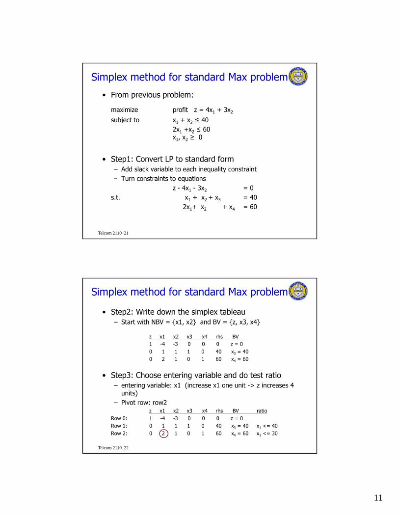
Simplex method for standard Max problem
• From previous problem:
maximize profit z = 4x1 + 3x2
subject to x1 + x2 ≤ 40subject to x1 + x2 ≤ 402x1 +x2 ≤ 60x1, x2 ≥ 0
• Step1: Convert LP to standard form– Add slack variable to each inequality constraint– Turn constraints to equations
Telcom 2110 21
Turn constraints to equationsz - 4x1 - 3x2 = 0
s.t. x1 + x2 + x3 = 402x1+ x2 + x4 = 60
Simplex method for standard Max problem
• Step2: Write down the simplex tableau – Start with NBV = {x1, x2} and BV = {z, x3, x4}
z x1 x2 x3 x4 rhs BVz x1 x2 x3 x4 rhs BV 1 -4 -3 0 0 0 z = 00 1 1 1 0 40 x3 = 40 0 2 1 0 1 60 x4 = 60
• Step3: Choose entering variable and do test ratio– entering variable: x1 (increase x1 one unit -> z increases 4
units)
Telcom 2110 22
units)– Pivot row: row2
z x1 x2 x3 x4 rhs BV ratioRow 0: 1 -4 -3 0 0 0 z = 0Row 1: 0 1 1 1 0 40 x3 = 40 x1 <= 40Row 2: 0 2 1 0 1 60 x4 = 60 x1 <= 30

12
Simplex method for standard Max problem
• Step4: Perform pivoting – Make coefficient of x1 in row2 to be one and all other rows to
be zeros– departing variable: x4 and BV = {z x3 x1}– departing variable: x4 and BV = {z, x3, x1}
z x1 x2 x3 x4 rhs BV 1 0 -1 0 2 120 z = 1200 0 0.5 1 -0.5 10 x3 = 10 0 1 0.5 0 0.5 30 x1 = 30
• Repeat step 3-4– entering variable: x2 (increase x2 one unit -> z increases one
Telcom 2110 23
entering variable: x2 (increase x2 one unit > z increases one unit)
– Pivot row: row1z x1 x2 s1 s2 rhs BV ratio
Row 0: 1 0 -1 0 2 120 z = 120Row 1: 0 0 0.5 1 -0.5 10 x3 = 10 x2 <= 20 Row 2: 0 1 0.5 0 0.5 30 x1 = 30 x2 <= 60
Simplex method for standard Max problem
• Optimal solution is reached– No new entering variable is found– x1 = 20, x2 = 20 with maximum profit at
z = 4(20) + 3(20) = $140 per week
z x1 x2 X3 X4 rhs BV ratio1 0 0 2 1 140 z = 1400 0 1 2 -1 20 x2 = 20 0 1 0 -1 1 20 x1 = 20
Telcom 2110 24

13
Solving LP problems
• Simplex method– Easy to use but to solve large problems need to use
computer• Many software packages implement LP simplex method
– General math/stats packages: Matlab, Excel, Mathematica etc.– Specialized optimization packages : LINDO, AMPL/CPLEX, XPRESS-
LP, etc.
• Consider three examples1. AMPL/CPLEX : modeling language (and software) for
designing and solving large complex LP/IP problems
Telcom 2110 25
designing and solving large complex LP/IP problems.2. MATLAB: General mathematics solver 3. MS EXCEL with SOLVER (standard spreadsheet tool)
Example: Simplex Algorithm• Look at the LP problem (slide 12,13) solved graphically:
Maximize:
Subject to:
CB XX 3025
4014012001 XX
• Adding slack variables (S1, S2, S3) and covert LP to standard form
Subject to: 4014012001 CB XX
60000 BX
40000 CX
Maximize:
Subject to:
25 30B CZ X X
1 200 1 140 40X X S
Telcom 2110 26
Subject to: 11 200 1 140 40B CX X S
2 6000BX S
3 4000CX S
1 2 3, , , , 0B CX X S S S
14
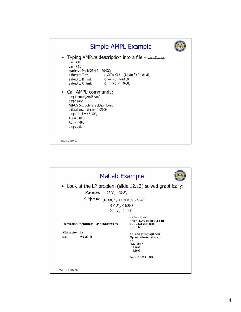
Simple AMPL Example
• Typing AMPL’s description into a file – prod0.modvar XB;var XC;maximize Profit: 25*XB + 30*XC;subject to Time: (1/200) * XB + (1/140) * XC <= 40;subject to B_limit: 0 <= XB <= 6000;subject to C_limit: 0 <= XC <= 4000;
• Call AMPL commands:ampl: model prod0.modampl: solve;MINOS 5.5: optimal solution found2 it ti bj ti 192000
Telcom 2110 27
2 iterations, objective 192000ampl: display XB, XC;XB = 6000XC = 1400ampl: quit
Matlab Example• Look at the LP problem (slide 12,13) solved graphically:
Maximize:
Subject to:CB XX 3025
4014012001 CB XX
60000 BX40000 CX
>> f = [-25 -30];>>A = [1/200 1/140; 1 0; 0 1];>> b = [40 6000 4000];>> b = b';
>> [x,fval]=linprog(f,A,b)Optimization terminated.
In Matlab formulate LP problems as
Minimize fxs.t. Ax ≤ b
Telcom 2110 28
px =1.0e+003 *
6.00001.4000
fval = -1.9200e+005

15
Steps in Implementing an LP Model in Excel
1. Organize the data for the model on the spreadsheet.
2 Reserve separate cells in the spreadsheet to2. Reserve separate cells in the spreadsheet to represent each decision variable in the model.
3. Create a formula in a cell in the spreadsheet that corresponds to the objective function.
4. For each constraint, create a formula in a separate cell in the spreadsheet that corresponds
Telcom 2110 29
to the left-hand side (LHS) of the constraint.• After entering LP model in spreadsheet, use
Solver to solve the model
EXCEL Example
• Two types of leather belts: deluxe and regular, each requires 1 sq. yard of leather
• Each week: only 40 sq yard leather & 60 hrs of labor skill available• Regular belt: 1 hr labor -> $3 profit• Deluxe belt: 2 hr labor -> $4 profit• Variable:
– x1 = # deluxe belts produced/wk– x2 = # regular belts produced/wk
• LP: maximize profit z = 4x1 + 3x2s.t. 2x1 +x2 <= 60, labor constraint
Telcom 2110 30
x1 + x2 <= 40, leather constraint x1, x2 >= 0, lower bound

16
Implementing LP model in a Spreadsheet
1. Organizing the data• Enter data into spreadsheet – in this example: unit profit, unit labor required,
unit leather required and available resource• Coefficient (e.g., in the objective function and constraints) and values (e.g., ( g , j ) ( g ,
RHS) of the model will be referred to or calculated from these data.• This makes the spreadsheet model more flexible to data changes.
Telcom 2110 31
2. Representing the decision variables• In this example, let cells B13 and C13 represent the decision variables X1 and X2.
• These cells should be shaded and outlined to visually distinguish them from other elements of the model.
S l ill d t i th ti l l f th ll
LP in MS EXCEL
• Solver will determine the optimal values for these cells
Telcom 2110 32

17
3. Representing the objective function.• Let Cell B16 represent an objective function: 4X1+3X2
- Enter the formula in cell B16 as = B7*B13+C7*C13
- Again, shaded and outlined to distinguish from other cells
LP in MS EXCEL
Telcom 2110 33
4. Representing the Constraints (1)• Create a formula in a cell that corresponds to the LHS or RHS of the constraint• Let cell B20 represent a LHS of labor constraint: 2X1+X
- Enter the formula in cell B20 as = B8*B13+C8*C13• Let cell D20 represent a RHS of labor constraint: 60
LP in MS EXCEL
- Enter the formula in cell D20 as = E8
Telcom 2110 34

18
4. Representing the Constraints (2)• Let cell B21represent a LHS of leather constraint: X1+X2
- Enter the formula in cell B21 as = B9*B13+C9*C13• Let cell D21 represent a RHS of leather constraint: 40
- Enter the formula in cell D21 as = E9
LP in MS EXCEL
Telcom 2110 35
Using Solver• After implementing an LP model in a spreadsheet, use Solver to solve the
model.
1. Invoking Solver in Excel• Choose the Solver command from the Tools menu• Then the Solver Parameters dialog boxes is displayed• Then the Solver Parameters dialog boxes is displayed
Telcom 2110 36

19
3. Defining the Changing Cells• Indicate which cells represent the decision variables in the model by
entering their locations in the By Changing Cells box
• In this example, cells B13 and C13 represent the decision variables
Using Solver
Telcom 2110 37
2. Defining the Target Cell • Specify the location of the cell that represents the objective function by entering
it (B16 in this example) in the Set Target Cell box• Cell B16 contains a formula representing the objective function• Select the Max button as in this example we want Solver to try to maximize
Using Solver
• Select the Max button, as in this example we want Solver to try to maximize this value (Select the Min button when you want to minimize the objective)
Telcom 2110 38
20
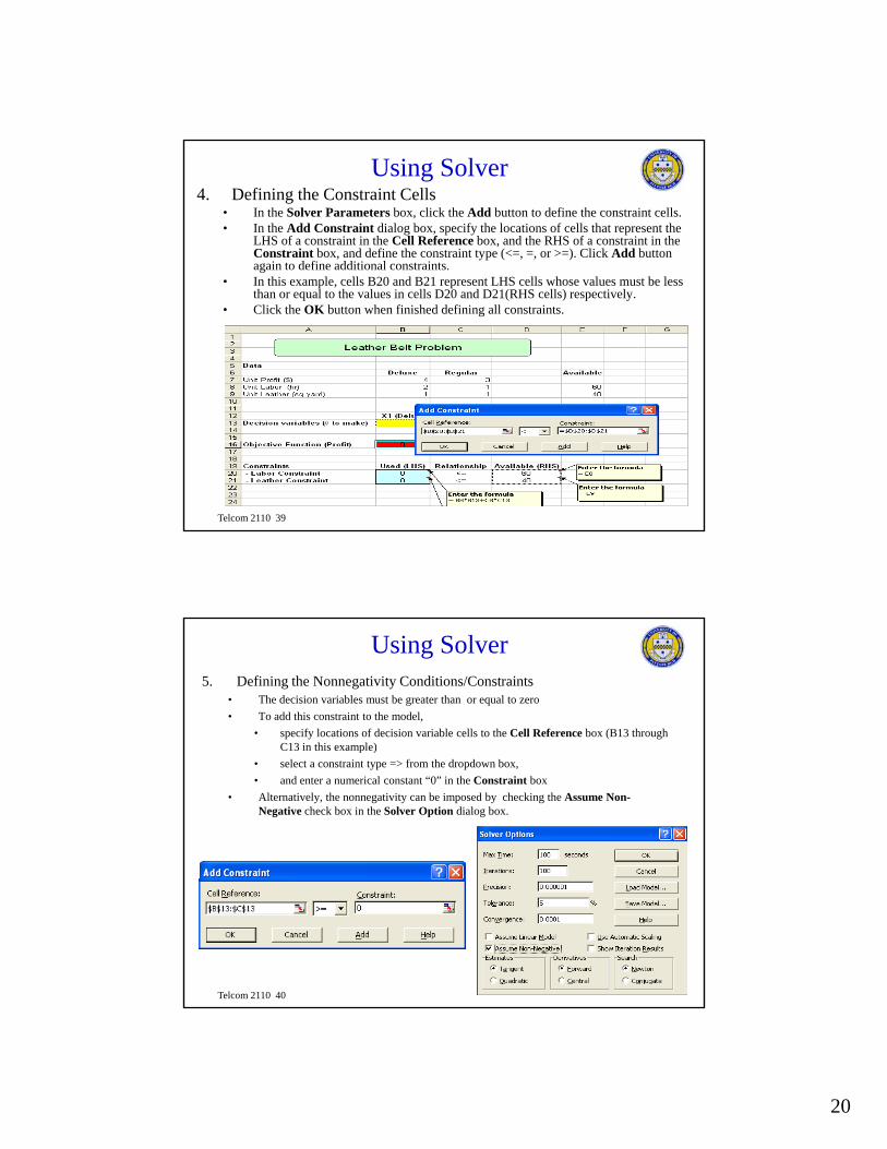
4. Defining the Constraint Cells• In the Solver Parameters box, click the Add button to define the constraint cells.• In the Add Constraint dialog box, specify the locations of cells that represent the
LHS of a constraint in the Cell Reference box, and the RHS of a constraint in the Constraint box, and define the constraint type (<=, =, or >=). Click Add button again to define additional constraints.
Using Solver
g• In this example, cells B20 and B21 represent LHS cells whose values must be less
than or equal to the values in cells D20 and D21(RHS cells) respectively.• Click the OK button when finished defining all constraints.
Telcom 2110 39
5. Defining the Nonnegativity Conditions/Constraints• The decision variables must be greater than or equal to zero
• To add this constraint to the model,
• specify locations of decision variable cells to the Cell Reference box (B13 through C13 in this example)
Using Solver
C13 in this example)
• select a constraint type => from the dropdown box,
• and enter a numerical constant “0” in the Constraint box
• Alternatively, the nonnegativity can be imposed by checking the Assume Non-Negative check box in the Solver Option dialog box.
Telcom 2110 40

21
6. Solving the model• Click the Solve button in the Solver Parameters dialog box to solve the
problem.• Optimal solutions: X1 = 20, X2 = 20• Optimal value(profit) = 140
Using the Solver
Telcom 2110 41
• Many problems in Network Design involve variables that are restricted to Integer Values – problems with such constraints are called Integer Programs or Mixed Integer Programs when some variables are integer and some are not
• Consider previous LP Example (slides 12-13)
Integer Programming
p p ( )– Assume that orders for bands and coils are placed (and filled) in 1,000s of
pounds only.– Although feasible region is greatly reduced, problem becomes much more
difficult.
• New Symbolic Model– Let the new decision variables be the number of 1000 pound “units” or
orders of bands and coils.
Maximize: XX 3000025000
Telcom 2110 42
Maximize:
Subject to:
CB XX 3000025000
4014010002001000 CB XX
,60 BX
,40 CX
integer
integer

22
Integer Programming
• Graphical Solution Method
2
4
6
Feasible integer solutions
Coils
$185K
Optimal integer solution ($185K)
X’C
Telcom 2110 43
00 2 4 6 8
Feasible integer solutions
Bands
X’B
Solving IP Problems
• Branch-and-Bound Procedure– The solution space consists of a tree of LP subproblems, in which each
integer variable is either fixed or its integrality constraint is “relaxed.”– The root node of the tree is the LP relaxation of the problem i e allThe root node of the tree is the LP relaxation of the problem, i.e. all
integer variables are relaxed.– The relaxation can result in an all integer solution, or a fractional
solution (some decision variables are non-integer).– If the solution of the relaxation has fractional-valued integer variables,
a fractional variable is selected for branching and two new subproblems are generated, each with more restrictive bounds on the branching variable.
– The subproblems can result in an all integer solution, an infeasible bl th f ti l l ti
Telcom 2110 44
problem or another fractional solution.– If the solution is fractional, the process is repeated.– Branches are “fathomed” if the subproblem is infeasible, the objective
value is worse than the current best integer solution or the subproblem gives an integer solution.

23
Solving MIP Problems
0
SP1:Bounds0<=XB<=60<=XC<=4
SolutionObj. = 192KXB = 6.00XC = 1.40
• Branch-and-Bound Tree (Example)
1 2
3 6
SP2:Bounds0<=XB<=60<=XC<=1
SolutionObj. = 180KXB = 6.00XC = 1.00
SP7:Bounds6<=XB<=62<=XC<=4
Solution*Infeasible
SP3:Bounds0<=XB<=62<=XC<=4
SolutionObj. = 189KXB = 5.14XC = 2.00
SP4:Bounds0<=XB<=52<=XC<=4
SolutionObj. = 188KXB = 5.00XC = 2 10
1
2
3
4
9
10
Telcom 2110 45
4 5
SP6:Bounds0<=XB<=53<=XC<=4
SolutionObj. = 183KXB = 3.71XC = 3.00
XC = 2.10
SP5:Bounds0<=XB<=52<=XC<=2
SolutionObj. = 185KXB = 5.00XC = 2.00
5
6 8
7
Branch-and-Bound (cont’d)
• Subproblem1: start with optimum LP solution
Coils
• Subproblem2: 0<=XB<=60<=XC<=1
Coils
Bands00 2 4 6 8
2
4
6
XC
XB=6, XC=1.4 => Z = $192K
Bands00 2 4 6 8
2
4
6
XC
XB=6, XC=1 => Z = $180K
Telcom 2110 46
0 2 4 6 8
XB
0 2 4 6 8
XB

24
Branch-and-Bound (cont’d)
• Subproblem3: 0<=XB<=62<=XC<=4
• Subproblem4: 0<=XB<=52<=XC<=4
Coils Coils
Bands00 2 4 6 8
2
4
6
XC
XB=5.14, XC=2 => Z = $188.57K XB=5, XC=2.1 => Z = $188K
00 2 4 6 8
2
4
6
XC
Telcom 2110 47
XB
0 2 4 6 8 0 2 4 6 8
XB
Branch-and-Bound (cont’d)
• Subproblem5: 0<=XB<=52<=XC<=2
• Subproblem6: 0<=XB<=53<=XC<=4
CoilsCoils
XB=3.7, XC=3 => Z = $182.5K
00 2 4 6 8
2
4
6
XC
Bands00 2 4 6 8
2
4
6
XC
XB=5, XC=2 => Z = $185K
Telcom 2110 48
0 2 4 6 8
XBXB
0 2 4 6 8

25
Branch-and-Bound (cont’d)
• Subproblem7: 6<=XB<=62<=XC<=4
Coils
Bands00 2 4 6 8
2
4
6
XC
NO Feasible Solution
Telcom 2110 49
XB
0 2 4 6 8
Matrix Expression of LP/IP Problems
• Why use it?– Most LP/IP problems are quite large and it becomes very
cumbersome to describe them by explicitly giving each linear f l d l f llfunction, equality, and inequality in full.
– It is desirable to model problems in a more general fashion (e.g. give an IP for optimally designing a mesh-restorable network in general as opposed to doing so for a specific network).
– Formulate with Matrix Vector or Sum format
Telcom 2110 50

26
Algebraic Expression of LP/IP Problems
• Basic Production Model (Revisited)
Problem name: prob lp Given: P a set of products
Algebraic ModelOriginal Model
Problem name: prob.lp
Maximize25 XB + 30 XC
Subject To0.005 XB + 0.007143 XC <= 40
Bounds0 <= XB <= 60000 <= XC <= 4000 Maximize: jj Xc
,P a set of products
hours available at the millb
tons per hour of product j, for eachja Pj
profit per ton of product j, for eachjc Pj
maximum tons of product j, for eachju Pj
Define variables: jX tons of product j to be made, for each Pj
Telcom 2110 51
End
Subject to:
Pj
bXaPj
jj
1
PjuX jj ,0
AMPL model
• Basic AMPL model (revisited) -prod0.modset P;param a {j in P};param b;param b;param c {j in P};param u {j in P};var X {j in P};maximize Total_Profit: sum {j in P} c[j] * X[j];subject to Time: sum {j in P} (1/a[j]) * X[j] <= b;subject to Limit {j in P}: 0 <= X[j] <= u[j];
• model data – prod0 dat
Telcom 2110 52
model data prod0.datset P := bands coils;param: a c u :=bands 200 25 6000coils 140 30 4000;param b := 40;

27
• Many optimization formulations and design tools for network design (WANDL, VPISystems, Opnet) – Optimization Techniques usually form the initial basis of the
formulation Often use a heuristic or meta heuristic solution techniques
Network Design
– Often use a heuristic or meta-heuristic solution techniques
• Formulation depends – Network layer (e.g., WDM, SONET, MPLS, etc.),– Technology (wired vs. wireless, etc.)– QoS requirements – Reliability goals– Other constraints
Telcom 2110 53
Network Design Optimization Models
• Network design problems– Network topology, Switch location, link capacity sizing,
routings, etc..• Good References
• M. Pioro and D. Medhi , Routing, Flow and Capacity Design in Communication and Computer Networks
• ITU Network Planning Manual Pt1 and Pt 2• Consider a couple of simple examples here –more later
– Max Flow Assignment (routing problem)A f l i
Telcom 2110 54
• Arc formulation• Path formulation
– Simple Network Design Model

28
Example: LP to find max flow between nodes 1-5 Edge capacities:
1
2 420 10
58
2
Max Flow LP Formulations
Define directional flow variables:
source
“trans-shipment nodes”
53 208
x42
1
24
x12
x13
x32 x23 x45
x24
Telcom 2110 55
sink53x35
Source: W. D. Grover, ECE 681, UofA, Fall 2004
To maximize (1 5) flow : /* using lp_solve syntax */
max: x12 + x13 ; /* (or x35 + x45) */
subject to constraints:
Max Flow LP Formulations (2)“transportation problem” or “arc-flow” approach
j
c1: x12 + x13 = x45 + x35 ; /* source = sink */
c2: x12 + x32 - x23 + x42 - x24 = 0 ; /* node 2 trans-shipment*/
c3: x13 + x23 - x32 - x35 = 0 ; /* node 3 trans-shipment*/
c4: x24 - x45 - x42 = 0 ; /* node 4 trans-shipment*/
x4224
x12x24
Telcom 2110 56
1
53
x13
x32 x23 x45
24
x35Source: W. D. Grover, ECE 681, UofA, Fall 2004

29
Continued....
Also subject to (capacity constraints):
x12 < 20 ;
Max Flow LP Formulations (3)“transportation problem” or “arc-flow” approach
220 10x13 < 8 ;
x24 < 10 ;
x42 < 10 ;
x23 < 2 ;
x32 < 2 ;
35 20
1
5
2 4
3
20 10
20
58
2
x42
1
24
x12
x32 x23 x
x24
Telcom 2110 57
x35 < 20 ;
x45 < 5 ; 53
x13
x23 x45
x35
Source: W. D. Grover, ECE 681, UofA, Fall 2004
Symbolically....
1,
max 1i E
x i
Max Flow LP Formulations (4)“transportation problem” or “arc-flow” approach
s.t. 1, 5,
1 5i E i E
x xi i
, ,
{ {1,5}}i j E i j E
x x i Nij ji
0 x s ij Eijij Where
Telcom 2110 58
ijijWhere:
E = set of edges that exist
N = set of nodes
sij = spare capacity on edge ij (= sji)
Source: W. D. Grover, ECE 681, UofA, Fall 2004

30
Symbolically....
15
maxi P
fi
Max Flow LP FormulationsAlternate approach: “flow assignment to routes” or “arc-path” approach
s.t.
15i P
kf s k Ei i k
Where:
E = set of edges that exist (indexed by k)
P 15= set of “eligible” distinct routes between nodes 1 and 5 (source-sink)
0 15f i Pi
Telcom 2110 59
15
sk = spare capacity on edge k
if the i th distinct route crosses span k. Zero otherwise
See Numerical Example posted on web pages
1ki
Source: W. D. Grover, ECE 681, UofA, Fall 2004
Identify all distinct routes between source- sink (set P15) ....
2f1
f4
Network Flow LP Formulations (6)“flow assignment to routes” or “arc-path” approach - example
Route associated fl i bl
Route associated fl i bl
1
5
2 4
3
1
5
2 4
3f2
f3
f4
Telcom 2110 60
flow variable
1-2-4-5 f1
1-2-3-5 f2
flow variable
1-3-5 f3
1-3-2-4-5 f4
Source: W. D. Grover, ECE 681, UofA, Fall 2004

31
To maximize (1 -> 5) flow :
max: f1 + f2 + f3 + f4 ;
subject to constraints:
Network Flow LP Formulations (7)“flow assignment to routes” or “arc-path” approach - example (2)
c1: f1 + f2 <= 20 ; /* link 12 capacity */
c2: f4 + f3 <= 8 ; /* link 13 capacity */
c3: f4 + f2 <= 2 ; /* link 23 capacity */
c4: f1 + f4 <= 10 ; /* link 24 */
2 4 2 4
f1f420 10
20 10
Telcom 2110 61
1
53
1
53f2
f320
58
20 10
20
58
2 2
Source: W. D. Grover, ECE 681, UofA, Fall 2004
What are the remaining constraints ? :
- for link 3-5 ... ?: c5: f3 + f2 <= 20; /*link 35 capacity */
Network Flow LP Formulations (8)“flow assignment to routes” or “arc-path” approach - example (2)
- for link 4-5 ... ?
1
2 4
1
2 4f41020
5
20 10
52 2
c6: f4 + f1 <= 5; /*link 45 capacity */
f1
(note this makes prior constraint f4 + f1<=10 redundant )
Telcom 2110 62
53 53f2
f320
8
208
Source: W. D. Grover, ECE 681, UofA, Fall 2004

32
• Note that the “indicator” parameters do not appear explicitly in the
executable model.
ki
Network Flow LP Formulations (9)“flow assignment to routes” or “arc-path” approach - example (3)
• Really they just represent our knowledge of the topology and the routes being considered.
• Implicitly above, we only wrote the flow variables that had non-zero coefficients.
Examples: 12 1 (flow1 crosses span 12)1 Hence f1 is in the first constraint
Telcom 2110 63
135 1 (flow3 crosses span 35)3 Hence f3 is in the fifth constraint, etc.
Source: W. D. Grover, ECE 681, UofA, Fall 2004See posted numerical example of arc-path approach
• indices– d=1,2,…,D set of demands (source-destination pairs)
– p=1,2,…,Pd possible paths for flows of demand d
Simple Network Design Problem
p , , , d p p
– e=1,2,…,E links
• Input parameters (constants) – hd offered traffic load of demand d
– ce upper bound on capacity of link e
– e unit (marginal) cost of link e
– edp = 1 if e belongs to path p realizing demand d; 0,
Telcom 2110 64
edp g p p g ; ,otherwise
• variables– xdp flow of demand d on path p
– ye capacity of each link

33
Capacitated flow allocation problemLP formulation – basic design
• Objective: minimize F(y) = e eye
• constraintsp xdp = hd d=1,2,…,D
d p edpxdp ye e=1,2,…,E
ye ce e=1,2,…,E
– flow and capacity variables are continuous and non-ti
Telcom 2110 65
negative
xdp 0, ye 0
This is an LP problem can solve using Simplex method See posted numerical example. Many variations tailor to specific network design problems see posted slides from D. Medhi book
Optimization Based Network Design Procedure
Input Data
Node Locations and potential locations Potential Links Traffic Demands Cost function/parameters
Network Design Optimizer
Find working path for traffic demands
Find backup paths for given failure scenarios
Network topology &Link capacity assignment
Technology, QoS requirements, etc
Survivability requirements
Network design strategy/Network optimization model
Telcom 2110 66
Output Results
Network Cost Network Topology Capacity of LinksWorking Paths Backup Paths

34
Complexity
• Real Network Design problems are quite large (have many variables and constraints)
– Graph Theory and Optimization Based algorithms for network design are complex – when can one use a technique?
C l it f l ith ll d t O( ) hi h d t th d• Complexity of an algorithm usually denotes O(.) which denotes the order of time growth in the algorithm as a function of problem variables
– Dijkstra’s Algorithm for SPT O(N log(N)) where N is number of nodes in graph
– Prim’s Algorithm for MST O(E log(N)) where N is # nodes, E # edges• Problems that can be solved by a deterministic algorithm in a polynomial
time complexity denoted P that is O(Nk) • Problems that can not be solved with P complexity denoted NP and don’t
scale well
Telcom 2110 67
– Linear Programming Problems have P complexity– Integer Programming Problems have NP complexity
• Still Branch and Bound can be used for small/medium problems !
• In general for NP problems use Sub-optimal solution algorithms (meta-heuristics – such as greedy alorithm, genetic algorithms, tabu search, etc.)
Summary•Basic Constrained optimization •Linear Programming
• Formulation • Graphical Solution• Simplex Method• Software Tools
• Integer Linear Programming• Branch and Bound Solution
• Network Design Models
Telcom 2110 68
g•Arc Flow formulation• Path formulation• Many variations in the literature tailored to specific design problem


![3. DUMMY VARIABLES, NONLINEAR VARIABLES AND SPECIFICATIONminiahn/ecn725/cn3_dummy.pdf · 2006-03-07 · DUMMY VARIABLES, NONLINEAR VARIABLES AND SPECIFICATION [1] DUMMY VARIABLES](https://img.pdfslide.net/doc/110x75/5b90b6d509d3f21c788c95bb/3-dummy-variables-nonlinear-variables-and-miniahnecn725cn3dummypdf-2006-03-07.jpg)