Optimization for Network Planning Includes slide materials developed by Wayne D. Grover, John Doucette, Dave Morley © Wayne D. Grover 2002, 2003 E E 681

Optimization for Network Optimization for Network PlanningPlanning

Includes slide materials developed by Wayne D. Grover, John Doucette, Dave Morley

© Wayne D. Grover 2002, 2003

E E 681 - Module 3

(version for book website)

E E 681 Lecture #3 © Wayne D. Grover 2002, 2003 2

Outline

• Optimization– Mathematical Programming– Linear Programming (LP)– Formulating LP Problems– Solving LP Problems– Integer Programming– Solving MIP Problems– Algebraic Expression of LP/IP Problems

• Mesh-Restoration Concept– Terminology– Spare Capacity Sharing– Spare Capacity Placement (SCP)– SCP Integer Programming problem


Mathematical Programming

1 T.W. Knowles, Management Science: Building and Using Models, Irwin, 1989.

Maximize (or minimize):

Subject to:

Constraints

Objective

• Definition– “A Mathematical Programming Model is a mathematical decision

model for planning (programming) decisions that optimize an objective function and satisfy limitations imposed by mathematical constraints.” 1

• General Symbolic Model

…

nxxxf 21,

1 1 2 1

2 1 2 2

, , ,

, , ,

n

n

g x x x b

g x x x b

1 2, , , m n mg x x x b

… where are the decision variables.nxxx 21,


Mathematical Programming

• Types of Mathematical Programs:– Linear Programs (LP): the objective and constraint functions are

linear and the decision variables are continuous.– Integer (Linear) Programs (IP): one or more of the decision

variables are restricted to integer values only and the functions are linear.

• Pure IP: all decision variables are integer.• Mixed IP (MIP): some decision variables are integer, others are

continuous.• 1/0 MIP: some or all decision variables are further restricted to be

valued either “1” or “0”.

– Nonlinear Programs: one or more of the functions is not linear.


Linear Programming

Maximize:

Subject to:

Constraints

Objective

Bounds

… where jjij cba ,, are the model parameters.

• General Symbolic Form

…

nnxcxcxc 2211

11 1 12 2 1 1

21 1 22 2 2 2

, ,

, ,

n n

n n

a x a x a x b

a x a x a x b

1 1 2 2 , ,

0 , 1, ,

m m mn n m

j

a x a x a x b

x j n


Linear Programming

• General Restrictions– All decision variables must be nonnegative,– Constant terms cannot appear on the LHS of a constraint.– No variable can appear on the RHS of a constraint.– No variable can appear more than once in a function, i.e. objective

or constraint.

• Steps for Formulating LP Models– Construct a verbal model.– Define the decision variables.– Construct the symbolic model.

.0jx


Formulating LP Problems

2 from, R. Fourer, D. Gay, B. Kernighan, AMPL, Boyd & Fraser, 1993, pp. 2-10.

Tons/ Profit/ hour ton

Bands 200 $25Coils 140 $30

Maximum tons: Bands 6,000Coils 4,000

• An example2

– A steel company must decide how to allocate production time on a rolling mill. The mill takes unfinished slabs of steel as input and can produce either of two products: bands and coils. The products come off the mill at different rates and also have different profitabilities:

– The weekly production that can be justified based on current and forecast orders are:



Maximize: total profitSubject to: total number of production hours 40

tons of bands produced 6,000tons of coils produced 4,000

• An example (cont’d)– The question facing the company is: If 40 hours of production time

are available, how many tons of bands and coils should be produced to bring in the greatest total profit?

• Constructing the Verbal model – Put the objective and constraints into words.– For constraints, use the form

{a verbal description of the LHS} {a relationship} {an RHS constant}


• Defining the Decision Variables – XB number of tons of bands produced.

– XC number of tons of coils produced.

• Construct the Symbolic Model


Maximize:

Subject to:

CB XX 3025

4014012001 CB XX

60000 BX

40000 CX


Solving LP Problems

Bands00 2000 4000 6000 8000

Coils

2000

4000

6000Constraints

Feasible region

00 2000 4000 6000 8000

Bands

Coils

2000

4000

6000220K

192K

120K

Profit

Optimal solution

Hours

• Graphical Solution Method


Solving LP Problems

Unique Optimal Solution Alternate Optimal Solutions

No Feasible Solution Unbounded Optimal Solution

• 4 Possible Outcomes


Solving LP Problems

• Simplex method– Efficient algorithm to solve LP problems by performing matrix

operations on the LP Tableau.– Developed by George Dantzig (1947).– Can be used to solve small LP problems by hand.

• AMPL and CPLEX– AMPL: modeling language (and software) for designing large and

complex LP/IP problems.– CPLEX: software package (“solver”) to solve large and complex

LP/IP problems.

• Sub-Optimal Algorithms (Heuristics)– Simulated annealing.– Genetic algorithms.– Tabu search.– Many others, often very specific to the type of problem.


Integer Programming

Maximize:

Subject to:

CB XX 3000025000

4014010002001000 CB XX

,60 BX

,40 CX

integer

integer

• Convert Example to Integer Program– Assume that orders for bands and coils are placed (and filled) in

1,000s of pounds only.– Although feasible region is greatly reduced, problem becomes much

more difficult.

• New Symbolic Model– Let the new decision variables be the number of 1000 pound “units”

or orders of bands and coils.


Integer Programming

00 2 4 6 8

2

4

6

Feasible integer solutions

Bands

Coils

$185K

Optimal integer solution ($185K)

• Graphical Solution Method


Solving MIP Problems

• Branch-and-Bound Procedure– The solution space consists of a tree of LP subproblems, in which each

integer variable is either fixed or its integrality constraint is “relaxed.”– The root node of the tree is the LP relaxation of the problem, i.e. all

integer variables are relaxed.– The relaxation can result in an all integer solution, or a fractional

solution (some decision variables are non-integer).– If the solution of the relaxation has fractional-valued integer variables, a

fractional variable is selected for branching and two new subproblems are generated, each with more restrictive bounds on the branching variable.

– The subproblems can result in an all integer solution, an infeasible problem or another fractional solution.

– If the solution is fractional, the process is repeated.– Branches are “fathomed” if the subproblem is infeasible, the objective

value is worse than the current best integer solution or the subproblem gives an integer solution.


Solving MIP Problems

0

1 2

3 6

4 5

Bounds0<=XB<=60<=XC<=1

SolutionObj. = 180KXB = 6.00XC = 1.00


Solution*Infeasible











1

2

3

4

5

6 8

7

9

10

• Branch-and-Bound Tree (Example)


Algebraic Expression of LP/IP Problems

• Why use it?– Most LP/IP problems are quite large and it becomes very

cumbersome to describe them by explicitly giving each linear function, equality, and inequality in full.

– It is desirable to model problems in a more general fashion (e.g. give an IP for optimally designing a mesh-restorable network in general as opposed to doing so for a specific network).


Algebraic Expression of LP/IP Problems

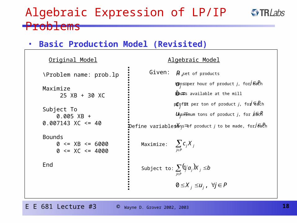
• Basic Production Model (Revisited)

\Problem name: prob.lp

Maximize 25 XB + 30 XC

Subject To 0.005 XB + 0.007143 XC <= 40

Bounds 0 <= XB <= 6000 0 <= XC <= 4000

End

Maximize:

Subject to:

Pj

jjXc

bXaPj

jj

1

PjuX jj ,0

Given: ,P a set of products

hours available at the millbtons per hour of product j, for eachja Pj

profit per ton of product j, for eachjc Pj

maximum tons of product j, for eachju Pj

Define variables: jX tons of product j to be made, for each Pj

Algebraic ModelOriginal Model


Example: LP/IP for Mesh-Restoration Design• Networks are Inherently Mesh-Like

• Distributed mesh-restoration exploits network connectivity to allow sharing of redundancy.

Level(3)North American Network


Spare Capacity Sharing

• Consider 2 different failure scenarios

X

X

– Restoration is allowed to follow multiple distinct routes.– Restoration route for both failure scenarios have several spans in

common.– Spare capacity on each span contributes to restorability of many

spans.


Spare Capacity Placement (SCP)

• Optimal Design– Objective is to find least costly way to place sufficient spare capacity

on a network such that all spans are fully restorable.– Can we use LP/IP?– Reference:

• M. Herzberg and S. J. Bye, “An Optimal Spare-Capacity Assignment Model for Survivable Networks with Hop Limits”, IEEE Globecom’94, 1994

• Integer Programming Approach– Objective Function:

• Minimize Cost of Spare Capacity Placement

– Constraints:• Each possible span failure has enough restoration flow for full

restoration.• Enough spare capacity exists on each span to accommodate restoration

flows.


SCP Integer Programming Problem

• Parameters (Inputs)– Cj: Cost of each unit of capacity on span j

– Li: Target Restoration level for span i (Li = 1 assumed)

– S: Number of spans in the network

– Pi: Number of eligible routes for restoration of span i

– wj: Number of working links (capacity units) on span j

i,jp: Equal to 1 if pth eligible route for span i uses span j

• Variables (Outputs)– fi

p: Restoration flow assigned to pth route for span i

– sj: Number of spare capacity units placed on span j


SCP Integer Programming Problem

• Objective Function:

• Subject To:

– 1.

– 2.

s

jjj sCMinimize

1

.,...,2,1 Si

jiSji .,...,2,1),(

ii

P

p

pi Lwf

i

1

iP

p

pi

pjij fs

1,

Documents

Optimization for Network Planning Includes slide materials developed by Wayne D. Grover, John Doucette, Dave Morley © Wayne D. Grover 2002, 2003 E E 681