Embed Size (px)
Citation preview
uptecf14052
Examensarbete 30 hpDecember 2014
Optimization for Train Energy Performance
Johan Brändström
Teknisk- naturvetenskaplig fakultet UTH-enheten Besöksadress: Ångströmlaboratoriet Lägerhyddsvägen 1 Hus 4, Plan 0 Postadress: Box 536 751 21 Uppsala Telefon: 018 – 471 30 03 Telefax: 018 – 471 30 00 Hemsida: http://www.teknat.uu.se/student
Abstract
Optimization for Train Energy Performace
Johan Brändström
In many studies efforts are made to decrease the energy consumption of trains by optimizing their drive style, e.g. accelerate and brake optimally and regenerate electricity when braking. In other studies the goal is to distribute the run time between stations in an optimal way to decrease the energy consumption, given a relatively simple drive style. In this report the goal is to combine these two energy saving methods to obtain as low energy consumption as possible. By coupling one software containing a drive style optimizer with another software which by different optimization methods calculates the optimal run time distribution on a given track this is accomplished. The study also contains a comparison between drive styles, with the goal to find a relatively simple but energy efficient drive style. Finally the dependence between run time distribution and energy consumption is further analysed.
The results show that by redistributing the run times the energy consumption can be decreased compared to previously existing time tables. They also show that a relatively simple drive style gives comparable energy consumption compared to the one obtained using a drive style optimizer. Finally the results show that the dependence between run time and energy consumption can be approximated with a simple second order equation.
ISSN: 1401-5757, UPTEC F14 052Examinator: Tomas NybergÄmnesgranskare: Per LötstedtHandledare: Astrid Herbst

Populärvetenskaplig sammanfattning
I många studier görs försök att sänka tågs energiförbrukning genom att optimera deras körstil, dvs gasaoch bromsa vid rätt tillfällen samt återmata elektricitet vid inbromsning. I andra studier är målet att dis-tribuera gångtiden mellan stationer på ett optimalt sätt för att sänka energiförbrukningen, givet en relativtenkel körstil. I den här rapporten är målet att kombinera dessa två energibesparande metoder för att fåen så låg energiförbrukning som möjligt. Detta görs genom att koppla ihop en mjukvara innehållandeen körstilsoptimerare med en annan mjukvara vars uppgift är att genom olika optimeringsmetoder räknaut optimal tidsdistribuering på en given bana. I studien ingår även en jämförelse mellan olika körstilari syftet att hitta en relativt enkel men energieffektiv körstil. Slutligen analyseras även relationen mellangångtidsdistribuering och energiförbrukning djupare.
Resultaten visar att genom att distribuera om gångtiderna kan energiförbrukningen sänkas jämfört medtidigare tidtabeller. De visar också att en relativt enkel körstil ger om något högre ändå jämförbar energiför-brukning med den från körstilsoptimeraren. Till slut visar resultaten att sambandet mellan gångtid ochenergiförbrukning kan approximeras med en enkel andragradsekvation.
1

Acknowledgements
I am using this opportunity to express my gratitude to everyone who supported me throughout the courseof this master thesis. I am sincerely grateful for the constructive help and path finding thoughts that havehelped guiding me to the final results of this report. I express my warm thanks to Astrid Herbst, JohanLundin, Rasmus Myklebust and Erik Wik for their expertise, support and guidance at Bombardier. Fur-thermore I thank Michel Chapuis, Cecilia Söderberg and Karl-Johan Åhs giving me personal and practicalsupport throughout the whole project. Finally I want to thank my girlfriend Monica Ricão, my parents Bir-gitta Brändström and Tomas Brändström and everyone else that has given me support to finish this project.
Thank you!
Johan Brändström
2
Contents
1 Populärvetenskaplig sammanfattning 1
2 Acknowledgements 2
3 Abbreviations and Units 5
4 Introduction 74.1 Background information . . . . . . . . . . . . . . . . . . . . . . . . . . . . . . . . . . . . . . . . 74.2 Objectives . . . . . . . . . . . . . . . . . . . . . . . . . . . . . . . . . . . . . . . . . . . . . . . . 74.3 Scope . . . . . . . . . . . . . . . . . . . . . . . . . . . . . . . . . . . . . . . . . . . . . . . . . . . 7
4.3.1 Limitations of the study . . . . . . . . . . . . . . . . . . . . . . . . . . . . . . . . . . . . 7
5 Theory 85.1 Time table optimization . . . . . . . . . . . . . . . . . . . . . . . . . . . . . . . . . . . . . . . . 85.2 TEP - Train Energy Performance . . . . . . . . . . . . . . . . . . . . . . . . . . . . . . . . . . . 85.3 Drive style optimization . . . . . . . . . . . . . . . . . . . . . . . . . . . . . . . . . . . . . . . . 8
5.3.1 All out Drive Style . . . . . . . . . . . . . . . . . . . . . . . . . . . . . . . . . . . . . . . 85.3.2 Energy saving techniques . . . . . . . . . . . . . . . . . . . . . . . . . . . . . . . . . . . 95.3.3 RMS currents in engine . . . . . . . . . . . . . . . . . . . . . . . . . . . . . . . . . . . . 10
5.4 Optimization algorithms . . . . . . . . . . . . . . . . . . . . . . . . . . . . . . . . . . . . . . . . 115.4.1 Design of Experiments - DOE . . . . . . . . . . . . . . . . . . . . . . . . . . . . . . . . . 115.4.2 Hill Climbing Algorithms . . . . . . . . . . . . . . . . . . . . . . . . . . . . . . . . . . . 125.4.3 Multi Objective Algorithms . . . . . . . . . . . . . . . . . . . . . . . . . . . . . . . . . . 14
5.5 Response surface method - RSM . . . . . . . . . . . . . . . . . . . . . . . . . . . . . . . . . . . 175.5.1 Response surface calculation models . . . . . . . . . . . . . . . . . . . . . . . . . . . . . 175.5.2 RSM validation methods . . . . . . . . . . . . . . . . . . . . . . . . . . . . . . . . . . . . 18
6 Methods 206.1 TEP set-up . . . . . . . . . . . . . . . . . . . . . . . . . . . . . . . . . . . . . . . . . . . . . . . . 206.2 Parametrization . . . . . . . . . . . . . . . . . . . . . . . . . . . . . . . . . . . . . . . . . . . . . 21
6.2.1 Optimization set-ups . . . . . . . . . . . . . . . . . . . . . . . . . . . . . . . . . . . . . . 226.2.2 AODC set-up . . . . . . . . . . . . . . . . . . . . . . . . . . . . . . . . . . . . . . . . . . 23
6.3 ModeFrontier set-up . . . . . . . . . . . . . . . . . . . . . . . . . . . . . . . . . . . . . . . . . . 266.3.1 Node configuration using DAS . . . . . . . . . . . . . . . . . . . . . . . . . . . . . . . . 266.3.2 Node configuration using all-out drive style . . . . . . . . . . . . . . . . . . . . . . . . 27
6.4 Time table optimization . . . . . . . . . . . . . . . . . . . . . . . . . . . . . . . . . . . . . . . . 286.5 RMS-impact investigation . . . . . . . . . . . . . . . . . . . . . . . . . . . . . . . . . . . . . . . 286.6 Response surface method . . . . . . . . . . . . . . . . . . . . . . . . . . . . . . . . . . . . . . . 28
6.6.1 RSM-validation . . . . . . . . . . . . . . . . . . . . . . . . . . . . . . . . . . . . . . . . . 29
7 Results 307.1 Optimization results using DAS . . . . . . . . . . . . . . . . . . . . . . . . . . . . . . . . . . . . 30
7.1.1 Test set-up using DAS . . . . . . . . . . . . . . . . . . . . . . . . . . . . . . . . . . . . . 307.1.2 Final set-up using DAS . . . . . . . . . . . . . . . . . . . . . . . . . . . . . . . . . . . . 31
7.2 Optimization preparation using AODC . . . . . . . . . . . . . . . . . . . . . . . . . . . . . . . 31
3
7.3 Comparison between drive styles . . . . . . . . . . . . . . . . . . . . . . . . . . . . . . . . . . . 357.3.1 RMS-impact . . . . . . . . . . . . . . . . . . . . . . . . . . . . . . . . . . . . . . . . . . . 36
7.4 Time table comparison . . . . . . . . . . . . . . . . . . . . . . . . . . . . . . . . . . . . . . . . . 377.5 RSM-analysis . . . . . . . . . . . . . . . . . . . . . . . . . . . . . . . . . . . . . . . . . . . . . . 39
7.5.1 Input parameter dependence according to the response surfaces . . . . . . . . . . . . . 397.5.2 RSM evaluation . . . . . . . . . . . . . . . . . . . . . . . . . . . . . . . . . . . . . . . . . 42
8 Discussion 468.1 Drive style comparison . . . . . . . . . . . . . . . . . . . . . . . . . . . . . . . . . . . . . . . . . 46
8.1.1 RMS-currents . . . . . . . . . . . . . . . . . . . . . . . . . . . . . . . . . . . . . . . . . . 468.2 Response surface method . . . . . . . . . . . . . . . . . . . . . . . . . . . . . . . . . . . . . . . 468.3 Time table optimization of GMTD using DAS . . . . . . . . . . . . . . . . . . . . . . . . . . . . 47
9 Outlook 489.1 Future time table optimization improvements . . . . . . . . . . . . . . . . . . . . . . . . . . . . 48
4

Abbreviations and Units
Table 3.1: Abbreviations
Abbreviation SignificanceSSH Secure ShellSET Server nameGUI Graphical User InterfaceTEP Train Energy PerformanceMF ModeFrontier
DAS Drive assistance systemAOD All-Out Drive style
AODC All-Out Drive style combined with CoastingGA Genetic Algorithm
DOE Design of ExperimentsULH Uniform Lattice Hypercube
MOGA Multi Objective Genetic AlgorithmRMS Root Mean SquareSVD Singular Value DecompositionNN Neural NetworksRBF Radial Basis Function
MAE Mean Absolute ErrorMRE Mean Relative ErrorAIC Akaike Information Criterion
GMTD Generic Metro Track Datajson File name extension of used in- and output files in TEPmat File name extension: Microsoft Access TableEC Energy Cost = Cost in Euro per kWhES Energy Saved = net energy saved per km
5
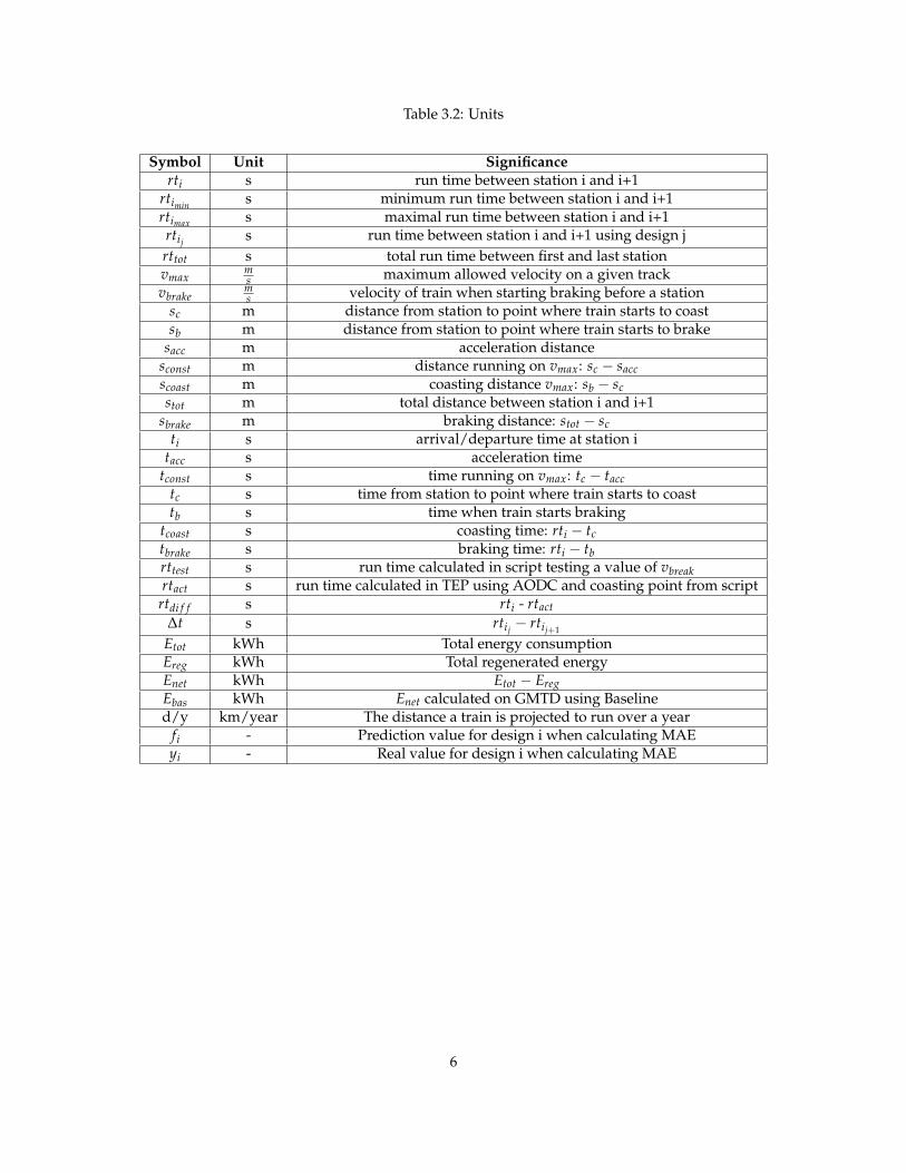
Table 3.2: Units
Symbol Unit Significancerti s run time between station i and i+1
rtimin s minimum run time between station i and i+1rtimax s maximal run time between station i and i+1rtij s run time between station i and i+1 using design jrttot s total run time between first and last stationvmax
ms maximum allowed velocity on a given track
vbrakems velocity of train when starting braking before a station
sc m distance from station to point where train starts to coastsb m distance from station to point where train starts to brake
sacc m acceleration distancesconst m distance running on vmax: sc − saccscoast m coasting distance vmax: sb − scstot m total distance between station i and i+1
sbrake m braking distance: stot − scti s arrival/departure time at station i
tacc s acceleration timetconst s time running on vmax: tc − tacc
tc s time from station to point where train starts to coasttb s time when train starts braking
tcoast s coasting time: rti − tctbrake s braking time: rti − tbrttest s run time calculated in script testing a value of vbreakrtact s run time calculated in TEP using AODC and coasting point from script
rtdi f f s rti - rtact∆t s rtij − rtij+1
Etot kWh Total energy consumptionEreg kWh Total regenerated energyEnet kWh Etot − EregEbas kWh Enet calculated on GMTD using Baselined/y km/year The distance a train is projected to run over a year
fi - Prediction value for design i when calculating MAEyi - Real value for design i when calculating MAE
6
Introduction
4.1 Background information
During the last couple of decades trains have become more and more important in the transportation sector,partly because of their comfort and relatively small pollution contribution compared to other transports.To be economically comparable to other transports it is important to always increase the efficiency of thetrains with regard to energy consumption. This can be done in different ways, e.g. by optimizing drivestyle using energy saving methods or by distributing the run time between stations optimally. Scheduleoptimization is of great importance to train operators when minimizing energy consumption. There aremany studies on energy optimization with regard to either drive style or time table optimization, but theyare rarely connected in one study [4].
An important part of Bombardier is to deliver Metros to customers. In order to be able to make acompetitive bid it is important to keep down the energy costs, since they are a big part of the total cost.
4.2 Objectives
By coupling an optimization software with an energy performance tool developed by Bombardier differentparametrizations are investigated in this paper. The two main objectives are schedule improvement anddrive style optimization. The schedule improvement aims at lowering the fuel consumption for trainsby optimizing the time distribution in the schedule. Desired is to find a drive style that is both easilyimplemented but also energy efficient. The drive styles are implemented in an energy performance tool,that also calculates the energy consumption between every station. The properties and accuracy of oneof the drive styles have not been thoroughly tested and the last part of this project aims at comparingthis optimizer with a simpler drive style. Furthermore the dependence of the input parameter run time isinvestigated with the help of different response surfaces. The accuracy of the algorithms used to create theresponse surfaces are investigated in different ways.
4.3 Scope
4.3.1 Limitations of the studyThe project was limited to make the scope of the project appropriate:
• When comparing drive styles three stations were used although if more time were given seven sta-tions would have been preferable.
• The time of the schedule optimization. A schedule optimization can theoretically run for weeks,which in this project was obviously not possible.
• The input parameter range was restricted. Increasing it drastically increases the calculation time andtherefore the range was chosen as wisely as possible to not loose accuracy in the results.
7
Theory
5.1 Time table optimization
There are different parameters that can affect a time table, and therefore different ways that a time tableoptimization can be made. In some studies the goal is to minimize the time table delays [1], while in otherdifferent constraints such as station capacities [2] or passenger waiting time [3] are used. Usually the timetables are set using these constraints and the energy optimization lies in the drive style [4]. In this report thefocus lies on lowering the energy consumption and optimizing the schedule and the drive style on a singletrack while outer circumstances such as delays or passenger flow are left out. The energy consumptioncalculations are made in one software, while the optimization is made in another. The basics of thesesoftware and drive style properties are explained in the following sections.
5.2 TEP - Train Energy Performance
The last couple of years Bombardier has developed a software called Train Energy Performance (TEP),which allows a detailed model of a rail vehicle to be simulated under a variety of conditions. The softwareutilizes detailed loss models for many of the electrical components, and has been validated against real-world energy consumption tests with satisfactory results. The program can be executed using complexinput data regarding the train, the track, surrounding environment, and drive style. Many train energyoptimization software use simplified models of the train (e.g purely mechanical models and constant train-set efficiency). The models in TEP are much more detailed with regard to the propulsion system losses,thus offering higher accuracy than many other software train models. With this software the models can bemade very precise, opening up to improved results in optimizations.
5.3 Drive style optimization
There are different ways the drive style of a train can be optimized to decrease energy consumption. Thischapter explains the most basic drive style often called all-out drive style (AOD). Some energy savingtechniques are explained that lay the ground for energy efficient driving which is described at the end ofthe section.
5.3.1 All out Drive StyleThe AOD is perhaps not famous for being the most energy efficient drive style. When a vehicle appliesAOD it drives at maximum allowed speed all the time, and it also utilizes maximum traction and brakingforce when accelerating and braking [6]. Consequently, the AOD yields the shortest travel time for anygiven track.
The AOD can be summarized in three steps that are shown in figure 5.1.
• Acceleration: The first part of the AOD consists of accelerating until the maximum allowed velocity onthe track is reached. The distance covered under this part is referred to as sacc while the correspondingtime is tacc.
• Constant Velocity: During the part when the train is running with maximum allowed velocity thecovered distance is sconst while the time is tconst:
8
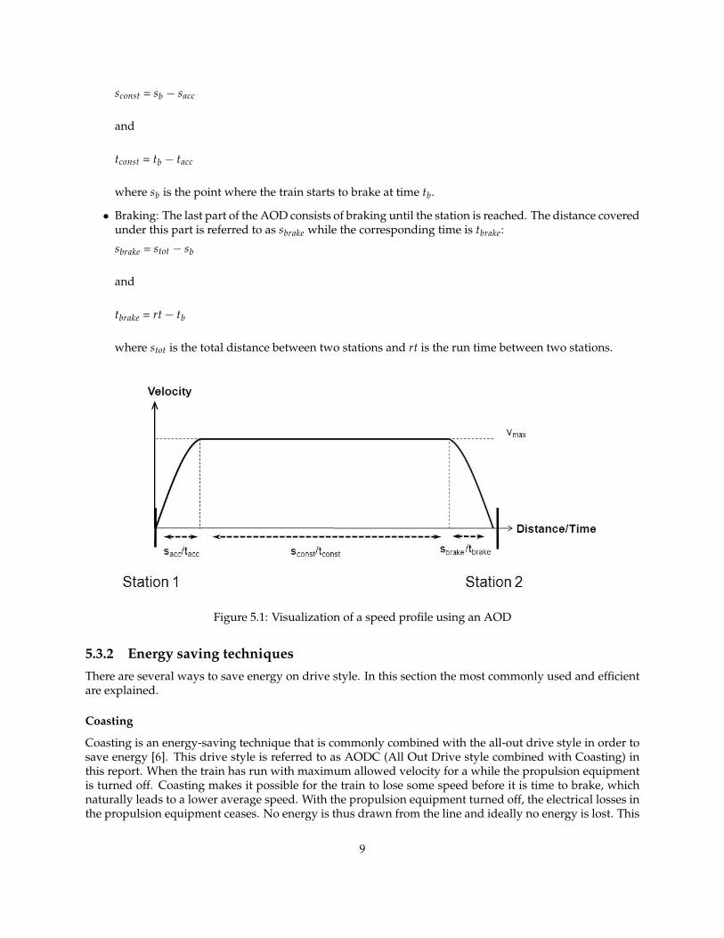
sconst = sb − sacc
and
tconst = tb − tacc
where sb is the point where the train starts to brake at time tb.
• Braking: The last part of the AOD consists of braking until the station is reached. The distance coveredunder this part is referred to as sbrake while the corresponding time is tbrake:
sbrake = stot − sb
and
tbrake = rt− tb
where stot is the total distance between two stations and rt is the run time between two stations.
Figure 5.1: Visualization of a speed profile using an AOD
5.3.2 Energy saving techniquesThere are several ways to save energy on drive style. In this section the most commonly used and efficientare explained.
Coasting
Coasting is an energy-saving technique that is commonly combined with the all-out drive style in order tosave energy [6]. This drive style is referred to as AODC (All Out Drive style combined with Coasting) inthis report. When the train has run with maximum allowed velocity for a while the propulsion equipmentis turned off. Coasting makes it possible for the train to lose some speed before it is time to brake, whichnaturally leads to a lower average speed. With the propulsion equipment turned off, the electrical losses inthe propulsion equipment ceases. No energy is thus drawn from the line and ideally no energy is lost. This
9
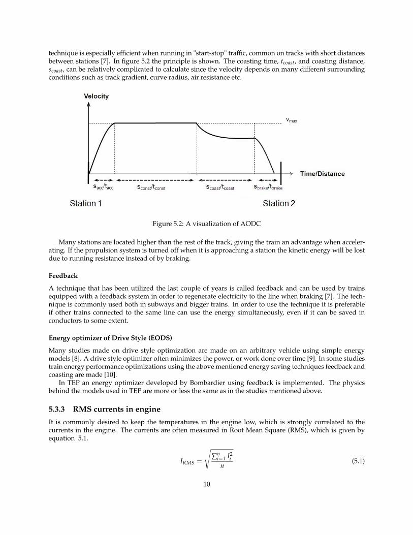
technique is especially efficient when running in "start-stop" traffic, common on tracks with short distancesbetween stations [7]. In figure 5.2 the principle is shown. The coasting time, tcoast, and coasting distance,scoast, can be relatively complicated to calculate since the velocity depends on many different surroundingconditions such as track gradient, curve radius, air resistance etc.
Figure 5.2: A visualization of AODC
Many stations are located higher than the rest of the track, giving the train an advantage when acceler-ating. If the propulsion system is turned off when it is approaching a station the kinetic energy will be lostdue to running resistance instead of by braking.
Feedback
A technique that has been utilized the last couple of years is called feedback and can be used by trainsequipped with a feedback system in order to regenerate electricity to the line when braking [7]. The tech-nique is commonly used both in subways and bigger trains. In order to use the technique it is preferableif other trains connected to the same line can use the energy simultaneously, even if it can be saved inconductors to some extent.
Energy optimizer of Drive Style (EODS)
Many studies made on drive style optimization are made on an arbitrary vehicle using simple energymodels [8]. A drive style optimizer often minimizes the power, or work done over time [9]. In some studiestrain energy performance optimizations using the above mentioned energy saving techniques feedback andcoasting are made [10].
In TEP an energy optimizer developed by Bombardier using feedback is implemented. The physicsbehind the models used in TEP are more or less the same as in the studies mentioned above.
5.3.3 RMS currents in engineIt is commonly desired to keep the temperatures in the engine low, which is strongly correlated to thecurrents in the engine. The currents are often measured in Root Mean Square (RMS), which is given byequation 5.1.
IRMS =
√∑n
i=1 I2i
n(5.1)
10
where n is the number of values of the current Ii given in different time steps.If the train has to use a lot of traction force, for example in a steep uphill, these currents can increase.
For some optimizations it might be of interest to keep the RMS-currents low in order to decrease the tem-perature in the engine.
5.4 Optimization algorithms
When solving an optimization problem the goal is to find either the maximum or minimum value of oneor more functions. The task can consist of one or more input parameters and the goal is to find the val-ues of these parameters that generate the highest or lowest goal functions. The more parameters and goalfunctions there are the more complicated the problem becomes. Optimizations with one goal functionare called single-objective optimizations, while optimizations with more than one goal function are calledmulti-objective optimizations [11].
Mathematically the functions that calculate the goal functions can be divided into linear and non-linear.In a linear function the extreme values lie at the end of the input parameter ranges and therefore the ex-treme values are not very complicated to find. The goal for an optimization problem is to find the globalextreme value, but in non-linear functions local extreme values can cause troubles. A good optimizationalgorithm has to be able to overcome this problem and to be fast at the same time. The following sectionsgo through the most common optimization algorithms solving both single and multi-objective problems.The structure of the theory is based on the structure in the optimization software ModeFrontier (MF).
5.4.1 Design of Experiments - DOEThe first step before running an optimization is to choose initial designs. This step is very important sinceit affects the speed of the convergence [12]. The choice of starting points is commonly referred to as Designof Experiments (DOE). There are many different ways to create a DOE and some are more sophisticatedthan others. A good sampling method manages to avoid clustering in order to make the algorithm testthe whole sampling space. If the starting points are clustered the risk of stopping at a local extreme pointduring the optimization increases. When running the DOE it is also important to have in mind how manystarting points that are needed. The desired number of points depends on which algorithms that are used,some need more than others. In the following paragraphs some of the most common sampling methodsare explained.
Random Sampling
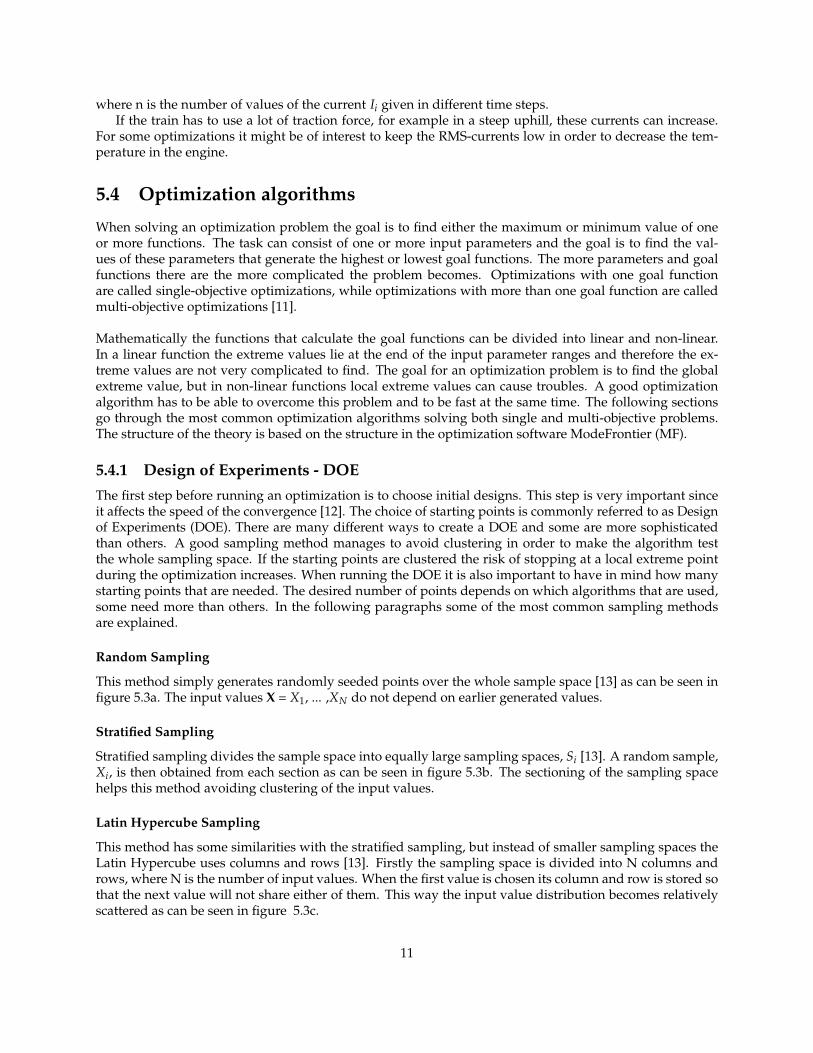
This method simply generates randomly seeded points over the whole sample space [13] as can be seen infigure 5.3a. The input values X = X1, ... ,XN do not depend on earlier generated values.
Stratified Sampling
Stratified sampling divides the sample space into equally large sampling spaces, Si [13]. A random sample,Xi, is then obtained from each section as can be seen in figure 5.3b. The sectioning of the sampling spacehelps this method avoiding clustering of the input values.
Latin Hypercube Sampling
This method has some similarities with the stratified sampling, but instead of smaller sampling spaces theLatin Hypercube uses columns and rows [13]. Firstly the sampling space is divided into N columns androws, where N is the number of input values. When the first value is chosen its column and row is stored sothat the next value will not share either of them. This way the input value distribution becomes relativelyscattered as can be seen in figure 5.3c.
11
(a) Example of randomsampling
(b) Example ofstratified sampling
(c) Example of LatinHypercube Sampling
Figure 5.3: Three different input parameter sampling types
Factorial designs
A factorial design is an example of a statistical design, which means that it is suitable for statistical anal-ysis [14]. It can either be a full factorial which means that every combination of the input parameters areinvestigated in order to find out how the output responds to changes of the input parameters. A reducedfactorial is commonly used when the number of designs becomes too large on a full factorial and the userwants to save time. The number of designs in a full factorial is equal to 2k where k is the number of inputparameters.
5.4.2 Hill Climbing AlgorithmsA common way of solving non-linear optimization problems is to use a hill climbing method. This methodaims at finding the global maximum of a function and is often used to solve single-objective problems [15].These kinds of algorithms have a tendency to "get stuck" at local extreme points. This can be avoidedby only using them on unimodal functions, which means that the function only has one extreme value inthe given region. SIMPLEX is a very efficient hill climbing method which has been combined with neweralgorithms in order to be used on multi-objective problems.
The SIMPLEX algorithm
A simplex is a geometrical figure that can consist of different number of points [15]. The SIMPLEX algo-rithm is started by creating a polytope consisting of N+1 vertices, where N is the number of dimensions ofthe input parameters [16]. This means that the number of input values from the DOE is N+1. The methoditerates the function values and moves the vertices of the polyhedron towards the optimal result by com-paring the values in the corners. The following example is a 2-dimensional problem, but the method can beused in any number of dimensions. In two dimensions the polytope becomes a triangle.
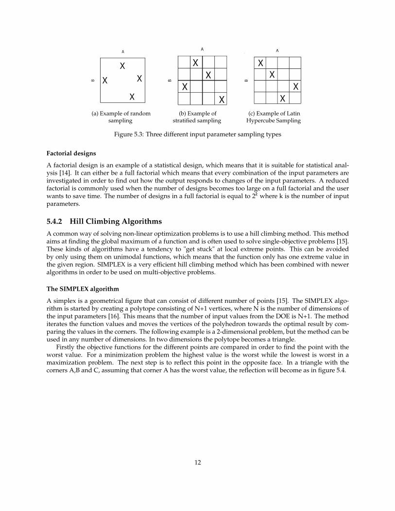
Firstly the objective functions for the different points are compared in order to find the point with theworst value. For a minimization problem the highest value is the worst while the lowest is worst in amaximization problem. The next step is to reflect this point in the opposite face. In a triangle with thecorners A,B and C, assuming that corner A has the worst value, the reflection will become as in figure 5.4.
12
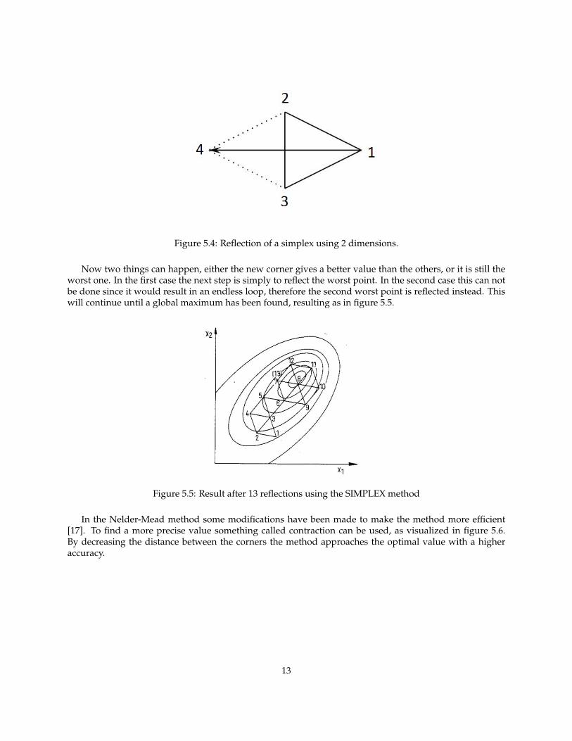
Figure 5.4: Reflection of a simplex using 2 dimensions.
Now two things can happen, either the new corner gives a better value than the others, or it is still theworst one. In the first case the next step is simply to reflect the worst point. In the second case this can notbe done since it would result in an endless loop, therefore the second worst point is reflected instead. Thiswill continue until a global maximum has been found, resulting as in figure 5.5.
Figure 5.5: Result after 13 reflections using the SIMPLEX method
In the Nelder-Mead method some modifications have been made to make the method more efficient[17]. To find a more precise value something called contraction can be used, as visualized in figure 5.6.By decreasing the distance between the corners the method approaches the optimal value with a higheraccuracy.
13
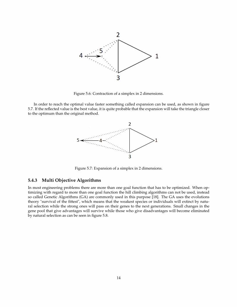
Figure 5.6: Contraction of a simplex in 2 dimensions.
In order to reach the optimal value faster something called expansion can be used, as shown in figure5.7. If the reflected value is the best value, it is quite probable that the expansion will take the triangle closerto the optimum than the original method.
Figure 5.7: Expansion of a simplex in 2 dimensions.
5.4.3 Multi Objective AlgorithmsIn most engineering problems there are more than one goal function that has to be optimized. When op-timizing with regard to more than one goal function the hill climbing algorithms can not be used, insteadso called Genetic Algorithms (GA) are commonly used in this purpose [18]. The GA uses the evolutionstheory "survival of the fittest", which means that the weakest species or individuals will extinct by natu-ral selection while the strong ones will pass on their genes to the next generations. Small changes in thegene pool that give advantages will survive while those who give disadvantages will become eliminatedby natural selection as can be seen in figure 5.8.
14
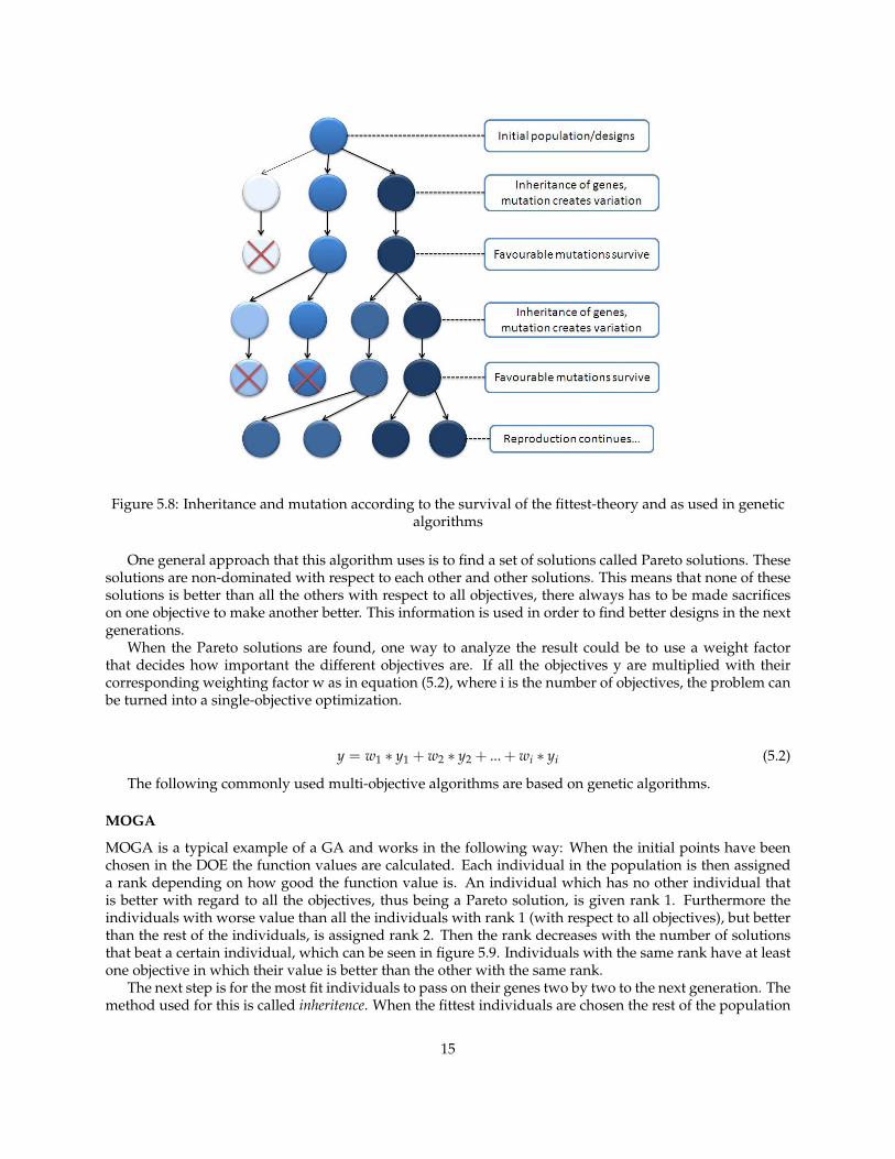
Figure 5.8: Inheritance and mutation according to the survival of the fittest-theory and as used in geneticalgorithms
One general approach that this algorithm uses is to find a set of solutions called Pareto solutions. Thesesolutions are non-dominated with respect to each other and other solutions. This means that none of thesesolutions is better than all the others with respect to all objectives, there always has to be made sacrificeson one objective to make another better. This information is used in order to find better designs in the nextgenerations.
When the Pareto solutions are found, one way to analyze the result could be to use a weight factorthat decides how important the different objectives are. If all the objectives y are multiplied with theircorresponding weighting factor w as in equation (5.2), where i is the number of objectives, the problem canbe turned into a single-objective optimization.
y = w1 ∗ y1 + w2 ∗ y2 + ... + wi ∗ yi (5.2)
The following commonly used multi-objective algorithms are based on genetic algorithms.
MOGA
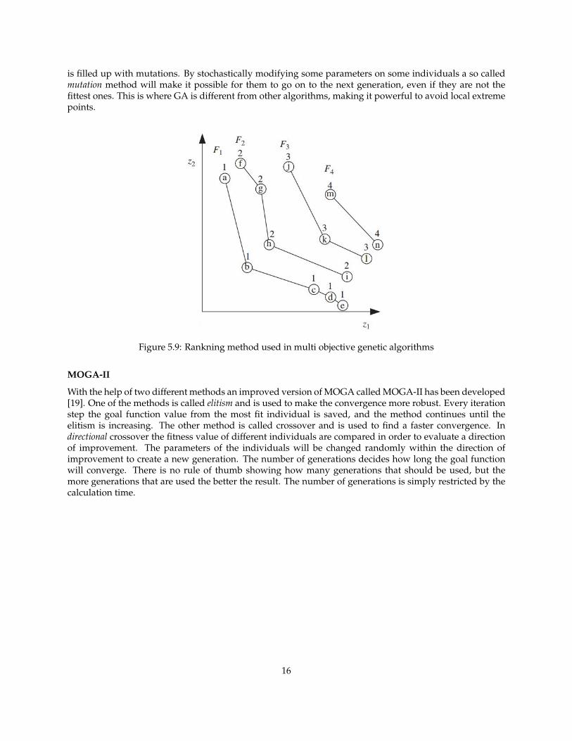
MOGA is a typical example of a GA and works in the following way: When the initial points have beenchosen in the DOE the function values are calculated. Each individual in the population is then assigneda rank depending on how good the function value is. An individual which has no other individual thatis better with regard to all the objectives, thus being a Pareto solution, is given rank 1. Furthermore theindividuals with worse value than all the individuals with rank 1 (with respect to all objectives), but betterthan the rest of the individuals, is assigned rank 2. Then the rank decreases with the number of solutionsthat beat a certain individual, which can be seen in figure 5.9. Individuals with the same rank have at leastone objective in which their value is better than the other with the same rank.
The next step is for the most fit individuals to pass on their genes two by two to the next generation. Themethod used for this is called inheritence. When the fittest individuals are chosen the rest of the population
15
is filled up with mutations. By stochastically modifying some parameters on some individuals a so calledmutation method will make it possible for them to go on to the next generation, even if they are not thefittest ones. This is where GA is different from other algorithms, making it powerful to avoid local extremepoints.
Figure 5.9: Rankning method used in multi objective genetic algorithms
MOGA-II
With the help of two different methods an improved version of MOGA called MOGA-II has been developed[19]. One of the methods is called elitism and is used to make the convergence more robust. Every iterationstep the goal function value from the most fit individual is saved, and the method continues until theelitism is increasing. The other method is called crossover and is used to find a faster convergence. Indirectional crossover the fitness value of different individuals are compared in order to evaluate a directionof improvement. The parameters of the individuals will be changed randomly within the direction ofimprovement to create a new generation. The number of generations decides how long the goal functionwill converge. There is no rule of thumb showing how many generations that should be used, but themore generations that are used the better the result. The number of generations is simply restricted by thecalculation time.
16
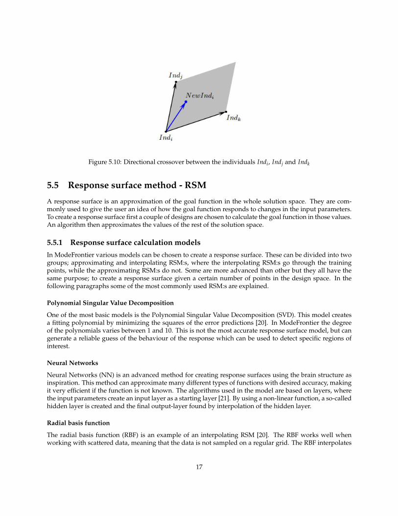
Figure 5.10: Directional crossover between the individuals Indi, Indj and Indk
5.5 Response surface method - RSM
A response surface is an approximation of the goal function in the whole solution space. They are com-monly used to give the user an idea of how the goal function responds to changes in the input parameters.To create a response surface first a couple of designs are chosen to calculate the goal function in those values.An algorithm then approximates the values of the rest of the solution space.
5.5.1 Response surface calculation modelsIn ModeFrontier various models can be chosen to create a response surface. These can be divided into twogroups; approximating and interpolating RSM:s, where the interpolating RSM:s go through the trainingpoints, while the approximating RSM:s do not. Some are more advanced than other but they all have thesame purpose; to create a response surface given a certain number of points in the design space. In thefollowing paragraphs some of the most commonly used RSM:s are explained.
Polynomial Singular Value Decomposition
One of the most basic models is the Polynomial Singular Value Decomposition (SVD). This model createsa fitting polynomial by minimizing the squares of the error predictions [20]. In ModeFrontier the degreeof the polynomials varies between 1 and 10. This is not the most accurate response surface model, but cangenerate a reliable guess of the behaviour of the response which can be used to detect specific regions ofinterest.
Neural Networks
Neural Networks (NN) is an advanced method for creating response surfaces using the brain structure asinspiration. This method can approximate many different types of functions with desired accuracy, makingit very efficient if the function is not known. The algorithms used in the model are based on layers, wherethe input parameters create an input layer as a starting layer [21]. By using a non-linear function, a so-calledhidden layer is created and the final output-layer found by interpolation of the hidden layer.
Radial basis function
The radial basis function (RBF) is an example of an interpolating RSM [20]. The RBF works well whenworking with scattered data, meaning that the data is not sampled on a regular grid. The RBF interpolates
17
the function using the input data and a certain radial function. There are five different radial functionsavailable in ModeFrontier. These are Gaussians (G), Duchon’s Polyharmonic Splines (PS), Hardy’s Multi-Quadrics (MQ), Inverse MultiQuardics (IMQ) and Wendland’s Compactly Supported C2 (W2). All of theseare commonly used in the field and could well work for the kind of problems that this report solves exceptthe W2 that can not be used with more than 5 dimensions.
5.5.2 RSM validation methodsThere are several ways to validate if a RSM is a good approximation of the solution to a problem. In thefollowing subsections some constants that can give information about the error are described as well as themore complex constant Akaike Information Criterion (AIC).
Mean absolute error
One of the most simple but efficient ways is to calculate the mean absolute error (MAE). The error, or thedifference between the real values and the calculated ones, is also commonly referred to as the residual.The absolute error is calculated as in equation 5.3.
ei = | fi − yi| (5.3)
Here fi is the function value of design i and yi the true value of design i. The absolute mean error is ob-tained by summing up the mean errors and dividing the result by the number of designs as in equation 5.4.
MAE =1n
n
∑i=1| fi − yi| =
1n
n
∑i=1|ei| (5.4)
Mean relative error
Another validation tool that can give additional information about the accuracy of a model is the meanrelative error, which is calculated as in equation 5.5.
MRE =100n
n
∑i=1
| fi − yi|yi
=100n
n
∑i=1
|ei|yi
(5.5)
Basically the absolute error is divided by the function value in every point and the total sum is multi-plied by 100 to obtain the answer in percent.
Akaike Information Criterion
One way to measure the quality of RSM is to use the Akaike information criterion (AIC). The AIC does notgive any information about how well the model fits the data, instead it estimates how much informationthat is lost when generating the model [22]. AIC is calculated as in equation 5.6.
AIC = 2k− 2 ln L (5.6)
where k is the number of input parameters and L is the likelihood function containing parameters from theresponse surface. AIC is always negative and a high absolute value indicates less data loss. This tool isespecially suited for comparing different models using the same input data.
18

Over-fitted functions
When making a polynomial-fitted curve a higher polynomial usually gives a smaller value of the MAE forthe training points [23]. However when the polynomial increases the risk for over-fitting occurs, whichmeans that the fitted curve starts to prioritize the accuracy in the training points rather then learning andgeneralize from them, which results in less accuracy in the new predicted data. If a function is over-fittedthis will be noticed in the AIC.
19
Methods
The first part of the project consisted of setting up the environment which is the foundation to both thetime table optimization and the drive style comparison. The train energy performance was optimized bycoupling TEP to the optimization software ModeFrontier (MF). TEP was installed on a Linux server whileMF was run from a workstation using Windows. By using a secure shell (SSH) MF was connected to theLinux server. After coupling the software, optimizations using different set-ups and parametrizations weremade and different drive styles compared. Lastly different response surfaces were made in order to find aninput parameter dependence, whereupon the response surface methods were examined.
In the following sections details about the set-ups, parametrizations and response surface methods areexplained.
6.1 TEP set-up
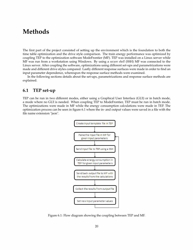
TEP can be run in two different modes, either using a Graphical User Interface (GUI) or in batch mode,a mode where no GUI is needed. When coupling TEP to ModeFrontier, TEP must be run in batch mode.The optimizations were made in MF while the energy consumption calculations were made in TEP. Theoptimization process can be seen in figure 6.1 where the in- and output values were saved in a file with thefile name extension "json".
Figure 6.1: Flow diagram showing the coupling between TEP and MF.
20
In TEP the drive style properties of the train can be chosen. The ones provided are AOD, AODC and onedrive style optimizer called Drive Assistance System (DAS). The details of these drive styles are explainedin section 6.2.
6.2 Parametrization
The two drive styles that were used in this project were DAS and AODC. The drive style optimizer DASchooses where the traction- and braking force is applied in order for the train to drive in an energy efficientmanner. This is done by testing all the available trajectories in every point of the track and choosing theones with least consumption for every point. When using DAS it is possible to manually set the time tablebefore running a simulation.
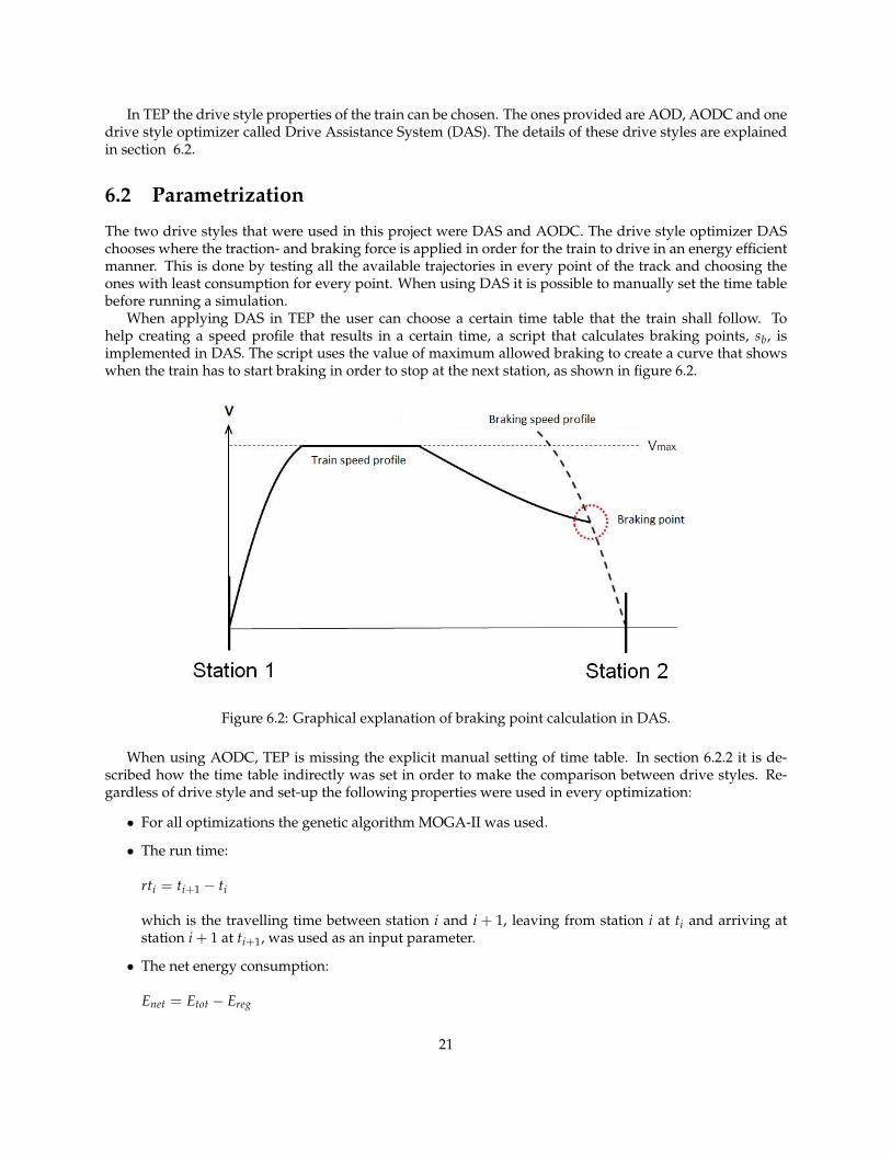
When applying DAS in TEP the user can choose a certain time table that the train shall follow. Tohelp creating a speed profile that results in a certain time, a script that calculates braking points, sb, isimplemented in DAS. The script uses the value of maximum allowed braking to create a curve that showswhen the train has to start braking in order to stop at the next station, as shown in figure 6.2.
Figure 6.2: Graphical explanation of braking point calculation in DAS.
When using AODC, TEP is missing the explicit manual setting of time table. In section 6.2.2 it is de-scribed how the time table indirectly was set in order to make the comparison between drive styles. Re-gardless of drive style and set-up the following properties were used in every optimization:
• For all optimizations the genetic algorithm MOGA-II was used.
• The run time:
rti = ti+1 − ti
which is the travelling time between station i and i + 1, leaving from station i at ti and arriving atstation i + 1 at ti+1, was used as an input parameter.
• The net energy consumption:
Enet = Etot − Ereg
21
where Etot is the total consumed energy and Ereg is the regenerated energy.
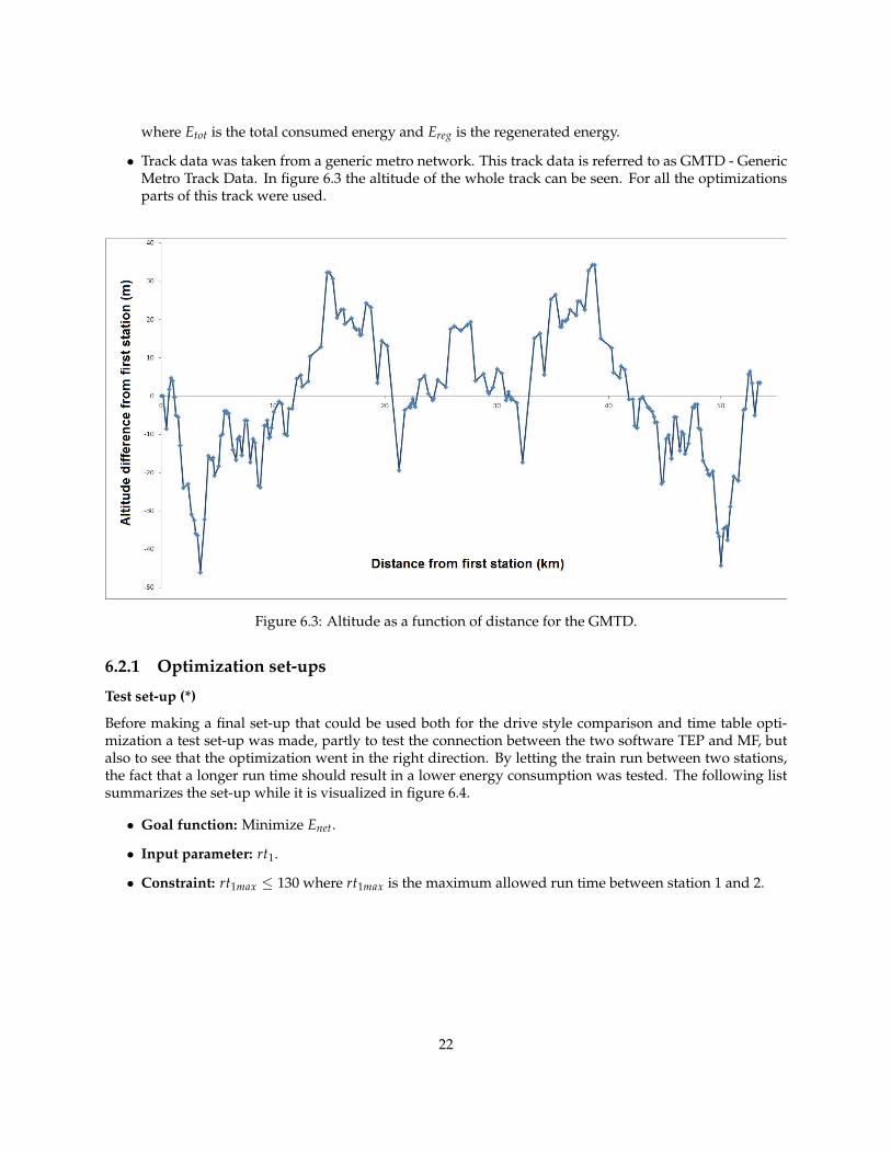
• Track data was taken from a generic metro network. This track data is referred to as GMTD - GenericMetro Track Data. In figure 6.3 the altitude of the whole track can be seen. For all the optimizationsparts of this track were used.
Figure 6.3: Altitude as a function of distance for the GMTD.
6.2.1 Optimization set-ups
Test set-up (*)
Before making a final set-up that could be used both for the drive style comparison and time table opti-mization a test set-up was made, partly to test the connection between the two software TEP and MF, butalso to see that the optimization went in the right direction. By letting the train run between two stations,the fact that a longer run time should result in a lower energy consumption was tested. The following listsummarizes the set-up while it is visualized in figure 6.4.
• Goal function: Minimize Enet.
• Input parameter: rt1.
• Constraint: rt1max ≤ 130 where rt1max is the maximum allowed run time between station 1 and 2.
22
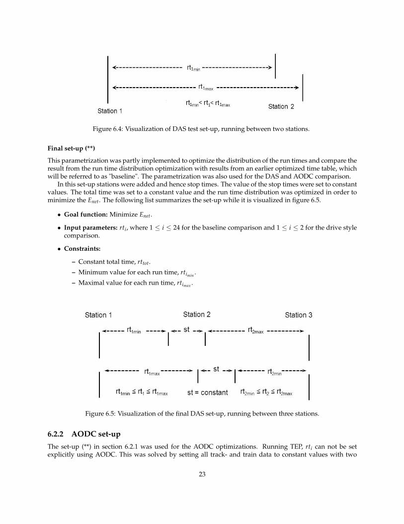
Figure 6.4: Visualization of DAS test set-up, running between two stations.
Final set-up (**)
This parametrization was partly implemented to optimize the distribution of the run times and compare theresult from the run time distribution optimization with results from an earlier optimized time table, whichwill be referred to as "baseline". The parametrization was also used for the DAS and AODC comparison.
In this set-up stations were added and hence stop times. The value of the stop times were set to constantvalues. The total time was set to a constant value and the run time distribution was optimized in order tominimize the Enet. The following list summarizes the set-up while it is visualized in figure 6.5.
• Goal function: Minimize Enet.
• Input parameters: rti, where 1 ≤ i ≤ 24 for the baseline comparison and 1 ≤ i ≤ 2 for the drive stylecomparison.
• Constraints:
– Constant total time, rttot.
– Minimum value for each run time, rtimin .
– Maximal value for each run time, rtimax .
Figure 6.5: Visualization of the final DAS set-up, running between three stations.
6.2.2 AODC set-upThe set-up (**) in section 6.2.1 was used for the AODC optimizations. Running TEP, rti can not be setexplicitly using AODC. This was solved by setting all track- and train data to constant values with two
23
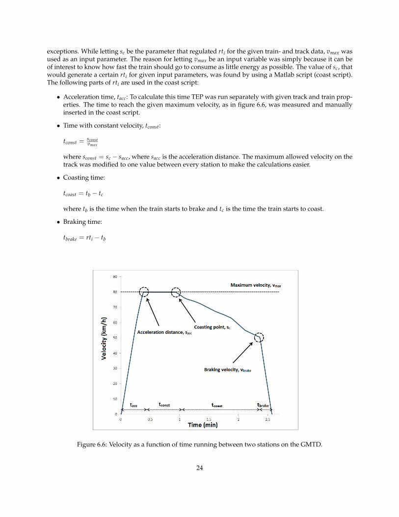
exceptions. While letting sc be the parameter that regulated rti for the given train- and track data, vmax wasused as an input parameter. The reason for letting vmax be an input variable was simply because it can beof interest to know how fast the train should go to consume as little energy as possible. The value of sc, thatwould generate a certain rti for given input parameters, was found by using a Matlab script (coast script).The following parts of rti are used in the coast script:
• Acceleration time, tacc: To calculate this time TEP was run separately with given track and train prop-erties. The time to reach the given maximum velocity, as in figure 6.6, was measured and manuallyinserted in the coast script.
• Time with constant velocity, tconst:
tconst =sconstvmax
where sconst = sc − sacc, where sacc is the acceleration distance. The maximum allowed velocity on thetrack was modified to one value between every station to make the calculations easier.
• Coasting time:
tcoast = tb − tc
where tb is the time when the train starts to brake and tc is the time the train starts to coast.
• Braking time:
tbrake = rti − tb
Figure 6.6: Velocity as a function of time running between two stations on the GMTD.
24
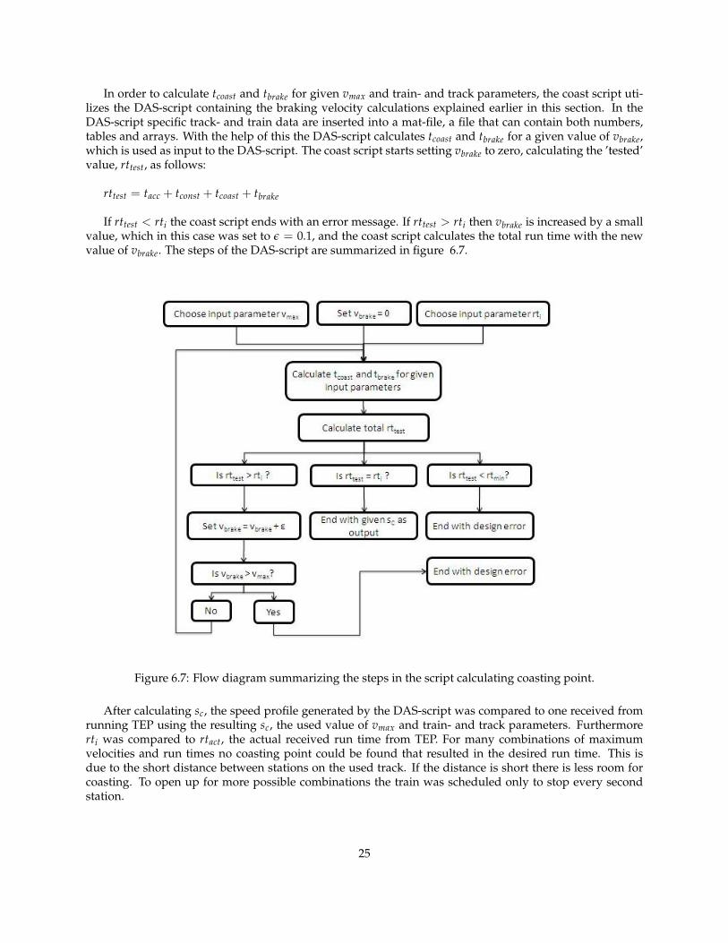
In order to calculate tcoast and tbrake for given vmax and train- and track parameters, the coast script uti-lizes the DAS-script containing the braking velocity calculations explained earlier in this section. In theDAS-script specific track- and train data are inserted into a mat-file, a file that can contain both numbers,tables and arrays. With the help of this the DAS-script calculates tcoast and tbrake for a given value of vbrake,which is used as input to the DAS-script. The coast script starts setting vbrake to zero, calculating the ’tested’value, rttest, as follows:
rttest = tacc + tconst + tcoast + tbrake
If rttest < rti the coast script ends with an error message. If rttest > rti then vbrake is increased by a smallvalue, which in this case was set to ε = 0.1, and the coast script calculates the total run time with the newvalue of vbrake. The steps of the DAS-script are summarized in figure 6.7.
Figure 6.7: Flow diagram summarizing the steps in the script calculating coasting point.
After calculating sc, the speed profile generated by the DAS-script was compared to one received fromrunning TEP using the resulting sc, the used value of vmax and train- and track parameters. Furthermorerti was compared to rtact, the actual received run time from TEP. For many combinations of maximumvelocities and run times no coasting point could be found that resulted in the desired run time. This isdue to the short distance between stations on the used track. If the distance is short there is less room forcoasting. To open up for more possible combinations the train was scheduled only to stop every secondstation.
25
6.3 ModeFrontier set-up
The optimization described in the previous chapter takes place in MF. All the commands in MF are con-trolled by nodes that each have different properties. One node was used for the coupling by using SSH-information. This way the input- and output files were sent back and forth between the Linux server andthe workstation. By running the terminal on the server through the SSH node TEP was started in batchmode. This way the energy consumption was calculated for every set of input parameters. In the followingsubsection the node configuration in MF is explained.
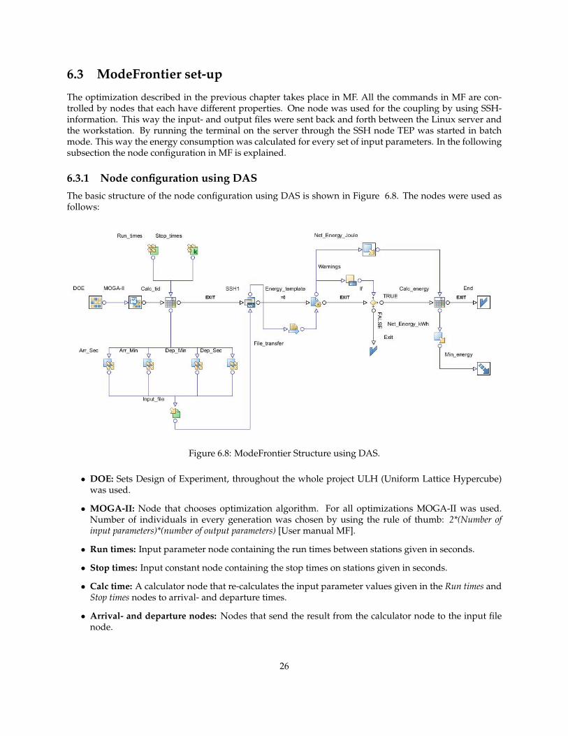
6.3.1 Node configuration using DASThe basic structure of the node configuration using DAS is shown in Figure 6.8. The nodes were used asfollows:
Figure 6.8: ModeFrontier Structure using DAS.
• DOE: Sets Design of Experiment, throughout the whole project ULH (Uniform Lattice Hypercube)was used.
• MOGA-II: Node that chooses optimization algorithm. For all optimizations MOGA-II was used.Number of individuals in every generation was chosen by using the rule of thumb: 2*(Number ofinput parameters)*(number of output parameters) [User manual MF].
• Run times: Input parameter node containing the run times between stations given in seconds.
• Stop times: Input constant node containing the stop times on stations given in seconds.
• Calc time: A calculator node that re-calculates the input parameter values given in the Run times andStop times nodes to arrival- and departure times.
• Arrival- and departure nodes: Nodes that send the result from the calculator node to the input filenode.
26
• Input file: A node that parses the input file that is send to the Linux server.
• SSH node: Contains SET-server name and login information.
• File transfer: Node that copies the output file from the SSH-server and sends it to a folder where itcan be found by the energy template node.
• Energy template: Searches the output file for DAS errors and Enet. This is done by setting a numbertag that has a relative position to a certain string.
• If-node: Node that discards designs that do not fulfil the constraints.
• Warnings: Node that informs the if-node if the design should be discarded or not.
• Calc energy: Calculates Enet in kWh.
• Net energy output nodes: Transfer the values of the energy to the next nodes.
• Min energy: Node that decides whether the goal function should be maximized or minimized.
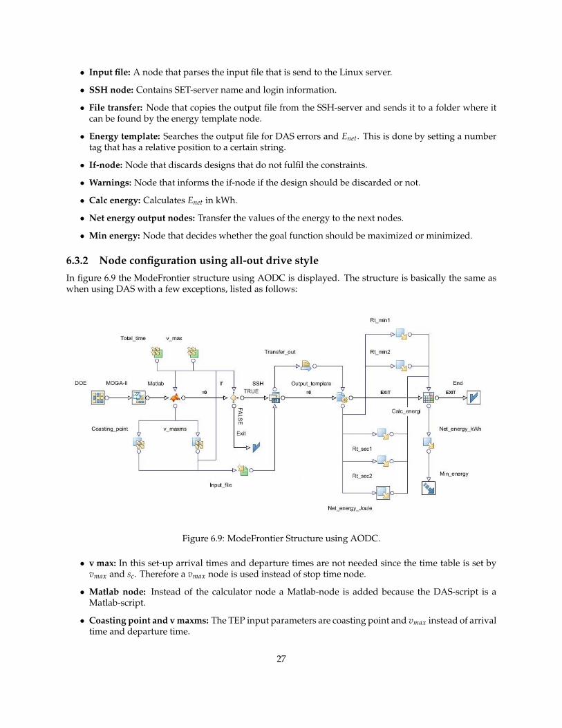
6.3.2 Node configuration using all-out drive styleIn figure 6.9 the ModeFrontier structure using AODC is displayed. The structure is basically the same aswhen using DAS with a few exceptions, listed as follows:
Figure 6.9: ModeFrontier Structure using AODC.
• v max: In this set-up arrival times and departure times are not needed since the time table is set byvmax and sc. Therefore a vmax node is used instead of stop time node.
• Matlab node: Instead of the calculator node a Matlab-node is added because the DAS-script is aMatlab-script.
• Coasting point and v maxms: The TEP input parameters are coasting point and vmax instead of arrivaltime and departure time.
27
• If node: Discards the designs found in Matlab-script with combinations of vmax and total time thatresult in an infeasible design.
• Rt min and Rt sec nodes: Nodes that were implemented in order to compare the desired run timeswith the resulting ones using the given coasting point and maximum velocity.
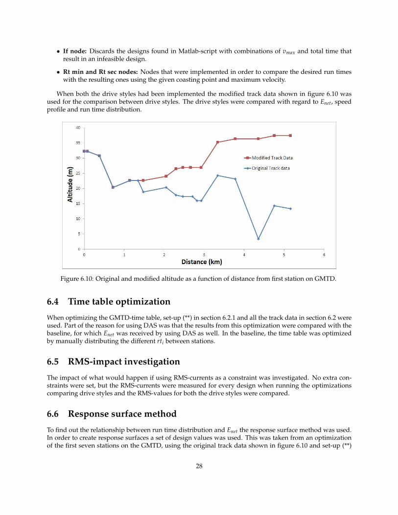
When both the drive styles had been implemented the modified track data shown in figure 6.10 wasused for the comparison between drive styles. The drive styles were compared with regard to Enet, speedprofile and run time distribution.
Figure 6.10: Original and modified altitude as a function of distance from first station on GMTD.
6.4 Time table optimization
When optimizing the GMTD-time table, set-up (**) in section 6.2.1 and all the track data in section 6.2 wereused. Part of the reason for using DAS was that the results from this optimization were compared with thebaseline, for which Enet was received by using DAS as well. In the baseline, the time table was optimizedby manually distributing the different rti between stations.
6.5 RMS-impact investigation
The impact of what would happen if using RMS-currents as a constraint was investigated. No extra con-straints were set, but the RMS-currents were measured for every design when running the optimizationscomparing drive styles and the RMS-values for both the drive styles were compared.
6.6 Response surface method
To find out the relationship between run time distribution and Enet the response surface method was used.In order to create response surfaces a set of design values was used. This was taken from an optimizationof the first seven stations on the GMTD, using the original track data shown in figure 6.10 and set-up (**)
28

in section 6.2.1. Normally a full factorial could be used in this purpose, but for the scope of this project theoptimization designs were used.
The MOGA-II optimization results were used to create the RSM-surface. Different RSM:s were made inorder to find one that correctly describes how Enet depends on the distribution of the run time. To examineif any polynomial dependence existed 1st, 2nd and 3rd order SVD polynomials were calculated. These werethen compared to the more advanced methods Neural Networks and Radial basis functions.
6.6.1 RSM-validationIn ModeFrontier there are various ways to validate a RSM-model. In this project the absolute mean errorbetween the original design data and the RSM:s were taken in regard. In addition to this the AIC wascalculated since it is a good way to validate statistical models. Firstly this was done using only the originaldata points from ULH and MOGA-II optimization. An additional test of the models was made by addingrandomly selected data points and investigate if the absolute mean error changed.
29
Results
7.1 Optimization results using DAS
In this section the results from set-up (*) and (**), explained in section 6.2, that were used to optimize GMTDtime table are shown. The used drive style throughout the whole section is DAS.
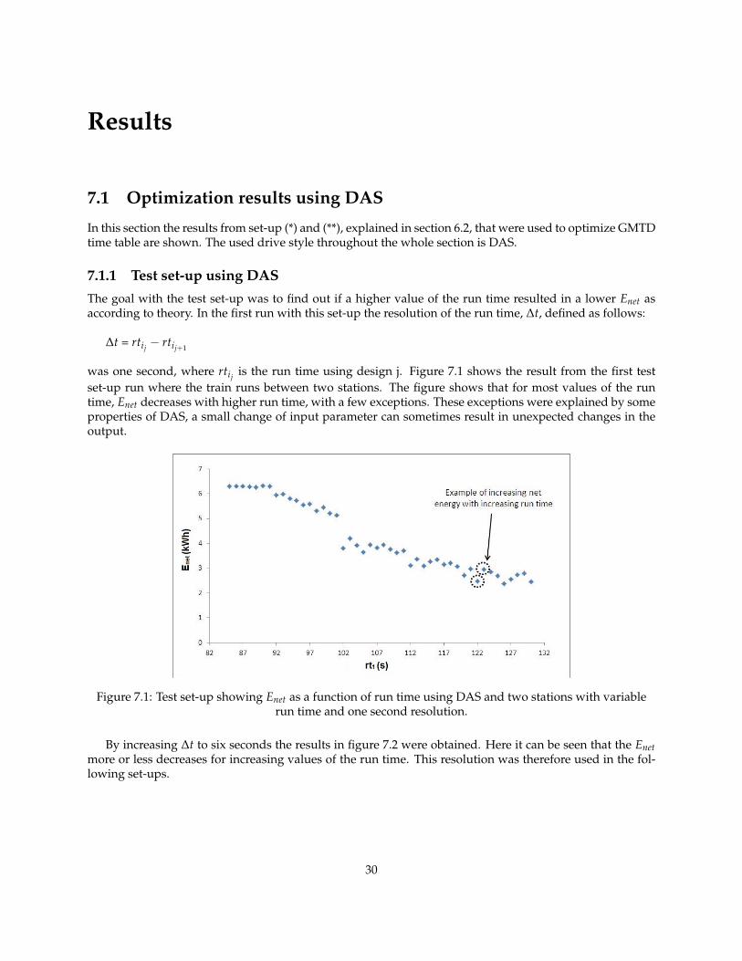
7.1.1 Test set-up using DASThe goal with the test set-up was to find out if a higher value of the run time resulted in a lower Enet asaccording to theory. In the first run with this set-up the resolution of the run time, ∆t, defined as follows:
∆t = rtij − rtij+1
was one second, where rtij is the run time using design j. Figure 7.1 shows the result from the first testset-up run where the train runs between two stations. The figure shows that for most values of the runtime, Enet decreases with higher run time, with a few exceptions. These exceptions were explained by someproperties of DAS, a small change of input parameter can sometimes result in unexpected changes in theoutput.
Figure 7.1: Test set-up showing Enet as a function of run time using DAS and two stations with variablerun time and one second resolution.
By increasing ∆t to six seconds the results in figure 7.2 were obtained. Here it can be seen that the Enetmore or less decreases for increasing values of the run time. This resolution was therefore used in the fol-lowing set-ups.
30
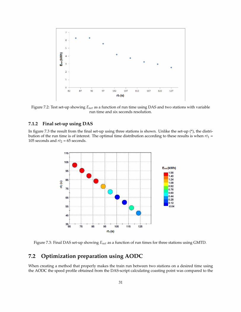
Figure 7.2: Test set-up showing Enet as a function of run time using DAS and two stations with variablerun time and six seconds resolution.
7.1.2 Final set-up using DASIn figure 7.3 the result from the final set-up using three stations is shown. Unlike the set-up (*), the distri-bution of the run time is of interest. The optimal time distribution according to these results is when rt1 =105 seconds and rt2 = 65 seconds.
Figure 7.3: Final DAS set-up showing Enet as a function of run times for three stations using GMTD.
7.2 Optimization preparation using AODC
When creating a method that properly makes the train run between two stations on a desired time usingthe AODC the speed profile obtained from the DAS-script calculating coasting point was compared to the
31
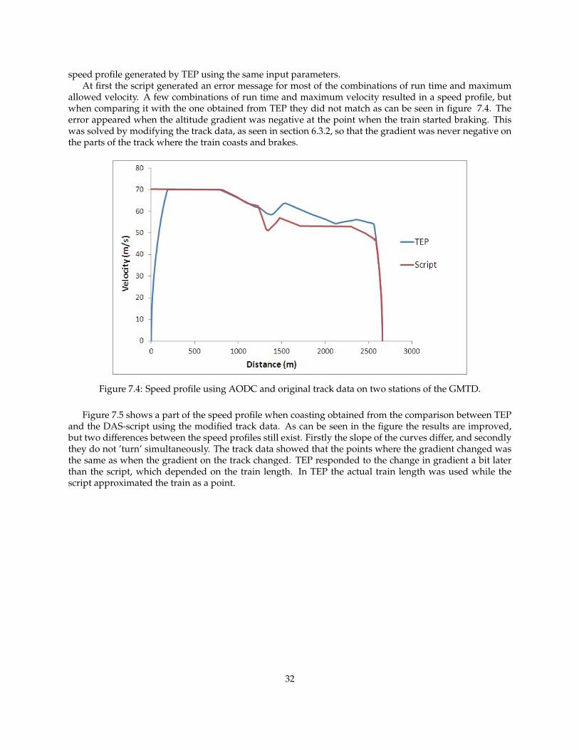
speed profile generated by TEP using the same input parameters.At first the script generated an error message for most of the combinations of run time and maximum
allowed velocity. A few combinations of run time and maximum velocity resulted in a speed profile, butwhen comparing it with the one obtained from TEP they did not match as can be seen in figure 7.4. Theerror appeared when the altitude gradient was negative at the point when the train started braking. Thiswas solved by modifying the track data, as seen in section 6.3.2, so that the gradient was never negative onthe parts of the track where the train coasts and brakes.
Figure 7.4: Speed profile using AODC and original track data on two stations of the GMTD.
Figure 7.5 shows a part of the speed profile when coasting obtained from the comparison between TEPand the DAS-script using the modified track data. As can be seen in the figure the results are improved,but two differences between the speed profiles still exist. Firstly the slope of the curves differ, and secondlythey do not ’turn’ simultaneously. The track data showed that the points where the gradient changed wasthe same as when the gradient on the track changed. TEP responded to the change in gradient a bit laterthan the script, which depended on the train length. In TEP the actual train length was used while thescript approximated the train as a point.
32
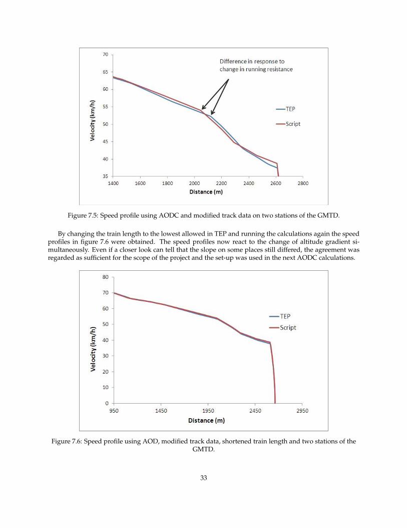
Figure 7.5: Speed profile using AODC and modified track data on two stations of the GMTD.
By changing the train length to the lowest allowed in TEP and running the calculations again the speedprofiles in figure 7.6 were obtained. The speed profiles now react to the change of altitude gradient si-multaneously. Even if a closer look can tell that the slope on some places still differed, the agreement wasregarded as sufficient for the scope of the project and the set-up was used in the next AODC calculations.
Figure 7.6: Speed profile using AOD, modified track data, shortened train length and two stations of theGMTD.
33
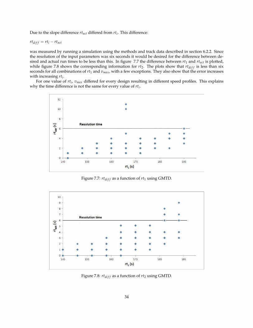
Due to the slope difference rtact differed from rti. This difference:
rtdi f f = rti − rtact
was measured by running a simulation using the methods and track data described in section 6.2.2. Sincethe resolution of the input parameters was six seconds it would be desired for the difference between de-sired and actual run times to be less than this. In figure 7.7 the difference between rt1 and rtact is plotted,while figure 7.8 shows the corresponding information for rt2. The plots show that rtdi f f is less than sixseconds for all combinations of rt1 and vmax, with a few exceptions. They also show that the error increaseswith increasing rti.
For one value of rti, vmax differed for every design resulting in different speed profiles. This explainswhy the time difference is not the same for every value of rti.
Figure 7.7: rtdi f f as a function of rt1 using GMTD.
Figure 7.8: rtdi f f as a function of rt2 using GMTD.
34
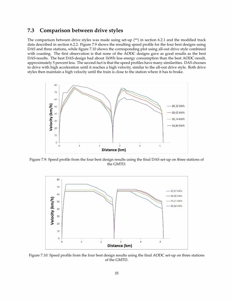
7.3 Comparison between drive styles
The comparison between drive styles was made using set-up (**) in section 6.2.1 and the modified trackdata described in section 6.2.2. Figure 7.9 shows the resulting speed profile for the four best designs usingDAS and three stations, while figure 7.10 shows the corresponding plot using all-out drive style combinedwith coasting. The first observation is that none of the AODC designs gave as good results as the bestDAS-results. The best DAS-design had about 1kWh less energy consumption than the best AODC-result,approximately 5 percent less. The second fact is that the speed profiles have many similarities. DAS choosesto drive with high acceleration until it reaches a high velocity, similar to the all-out drive style. Both drivestyles then maintain a high velocity until the train is close to the station where it has to brake.
Figure 7.9: Speed profile from the four best design results using the final DAS set-up on three stations ofthe GMTD.
Figure 7.10: Speed profile from the four best design results using the final AODC set-up on three stationsof the GMTD.
35
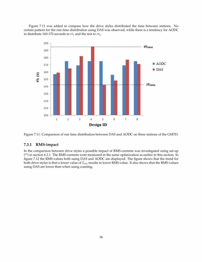
Figure 7.11 was added to compare how the drive styles distributed the time between stations. Nocertain pattern for the run time distribution using DAS was observed, while there is a tendency for AODCto distribute 160-170 seconds to rt1 and the rest to rt2.
Figure 7.11: Comparison of run time distribution between DAS and AODC on three stations of the GMTD.
7.3.1 RMS-impactIn the comparison between drive styles a possible impact of RMS-currents was investigated using set-up(**) in section 6.2.1. The RMS-currents were measured in the same optimization as earlier in this section. Infigure 7.12 the RMS-values both using DAS and AODC are displayed. The figure shows that the trend forboth drive styles is that a lower value of Enet results in lower RMS-value. It also shows that the RMS-valuesusing DAS are lower than when using coasting.
36
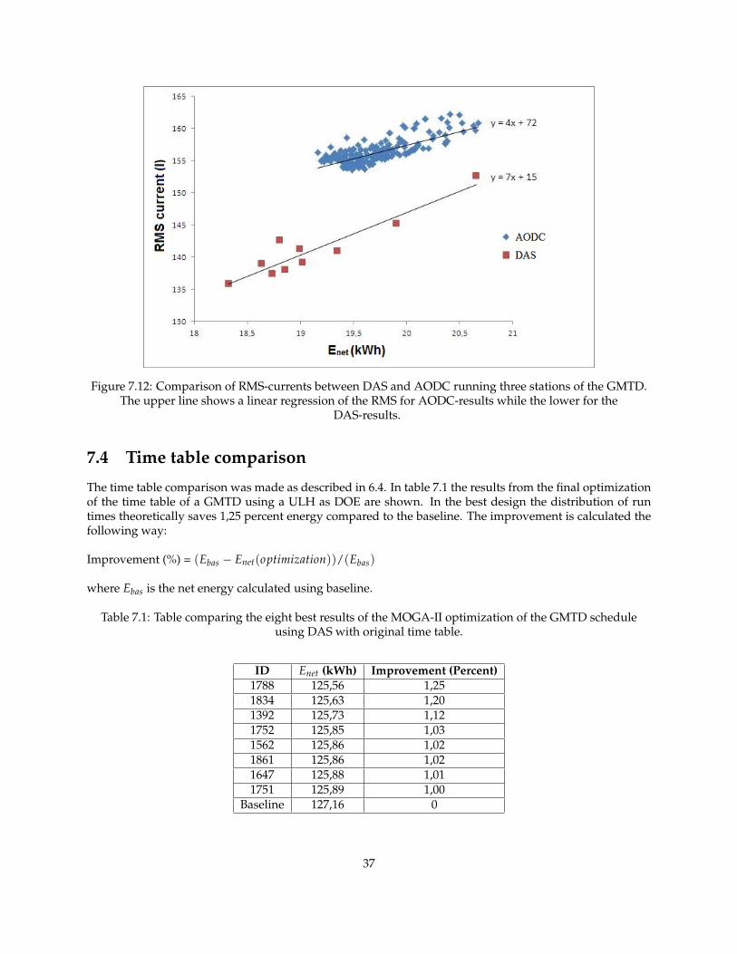
Figure 7.12: Comparison of RMS-currents between DAS and AODC running three stations of the GMTD.The upper line shows a linear regression of the RMS for AODC-results while the lower for the
DAS-results.
7.4 Time table comparison
The time table comparison was made as described in 6.4. In table 7.1 the results from the final optimizationof the time table of a GMTD using a ULH as DOE are shown. In the best design the distribution of runtimes theoretically saves 1,25 percent energy compared to the baseline. The improvement is calculated thefollowing way:
Improvement (%) = (Ebas − Enet(optimization))/(Ebas)
where Ebas is the net energy calculated using baseline.
Table 7.1: Table comparing the eight best results of the MOGA-II optimization of the GMTD scheduleusing DAS with original time table.
ID Enet (kWh) Improvement (Percent)1788 125,56 1,251834 125,63 1,201392 125,73 1,121752 125,85 1,031562 125,86 1,021861 125,86 1,021647 125,88 1,011751 125,89 1,00
Baseline 127,16 0
37
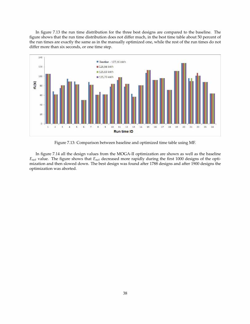
In figure 7.13 the run time distribution for the three best designs are compared to the baseline. Thefigure shows that the run time distribution does not differ much, in the best time table about 50 percent ofthe run times are exactly the same as in the manually optimized one, while the rest of the run times do notdiffer more than six seconds, or one time step.
Figure 7.13: Comparison between baseline and optimized time table using MF.
In figure 7.14 all the design values from the MOGA-II optimization are shown as well as the baselineEnet value. The figure shows that Enet decreased more rapidly during the first 1000 designs of the opti-mization and then slowed down. The best design was found after 1788 designs and after 1900 designs theoptimization was aborted.
38
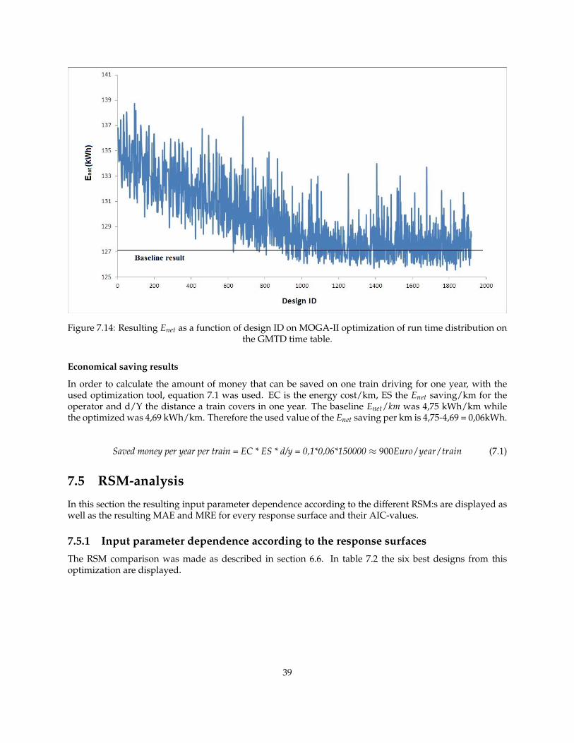
Figure 7.14: Resulting Enet as a function of design ID on MOGA-II optimization of run time distribution onthe GMTD time table.
Economical saving results
In order to calculate the amount of money that can be saved on one train driving for one year, with theused optimization tool, equation 7.1 was used. EC is the energy cost/km, ES the Enet saving/km for theoperator and d/Y the distance a train covers in one year. The baseline Enet/km was 4,75 kWh/km whilethe optimized was 4,69 kWh/km. Therefore the used value of the Enet saving per km is 4,75-4,69 = 0,06kWh.
Saved money per year per train = EC * ES * d/y = 0,1*0,06*150000 ≈ 900Euro/year/train (7.1)
7.5 RSM-analysis
In this section the resulting input parameter dependence according to the different RSM:s are displayed aswell as the resulting MAE and MRE for every response surface and their AIC-values.
7.5.1 Input parameter dependence according to the response surfacesThe RSM comparison was made as described in section 6.6. In table 7.2 the six best designs from thisoptimization are displayed.
39
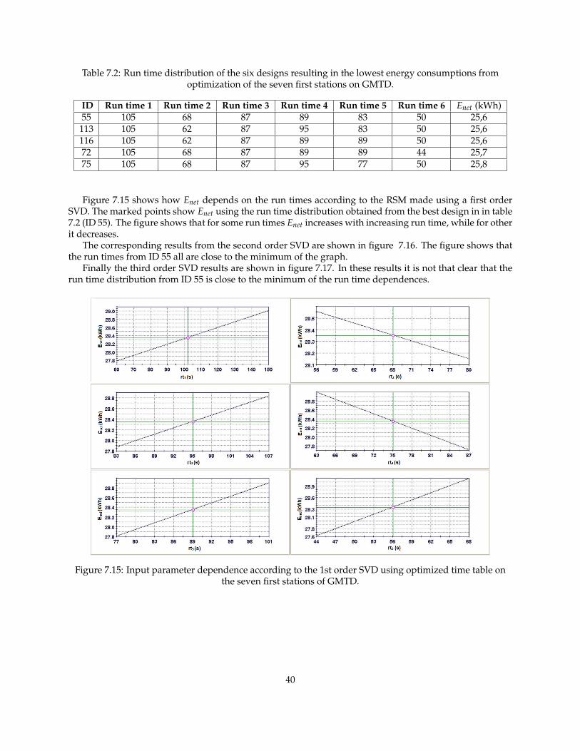
Table 7.2: Run time distribution of the six designs resulting in the lowest energy consumptions fromoptimization of the seven first stations on GMTD.
ID Run time 1 Run time 2 Run time 3 Run time 4 Run time 5 Run time 6 Enet (kWh)55 105 68 87 89 83 50 25,6113 105 62 87 95 83 50 25,6116 105 62 87 89 89 50 25,672 105 68 87 89 89 44 25,775 105 68 87 95 77 50 25,8
Figure 7.15 shows how Enet depends on the run times according to the RSM made using a first orderSVD. The marked points show Enet using the run time distribution obtained from the best design in in table7.2 (ID 55). The figure shows that for some run times Enet increases with increasing run time, while for otherit decreases.
The corresponding results from the second order SVD are shown in figure 7.16. The figure shows thatthe run times from ID 55 all are close to the minimum of the graph.
Finally the third order SVD results are shown in figure 7.17. In these results it is not that clear that therun time distribution from ID 55 is close to the minimum of the run time dependences.
Figure 7.15: Input parameter dependence according to the 1st order SVD using optimized time table onthe seven first stations of GMTD.
40
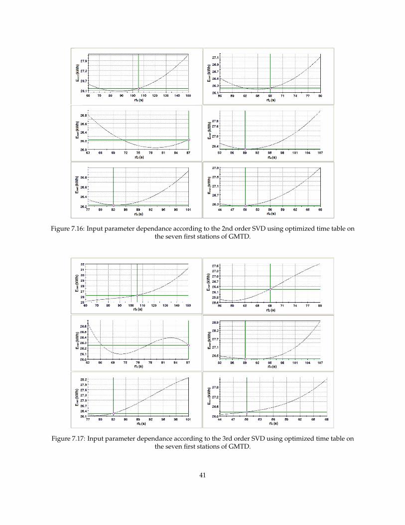
Figure 7.16: Input parameter dependance according to the 2nd order SVD using optimized time table onthe seven first stations of GMTD.
Figure 7.17: Input parameter dependance according to the 3rd order SVD using optimized time table onthe seven first stations of GMTD.
41
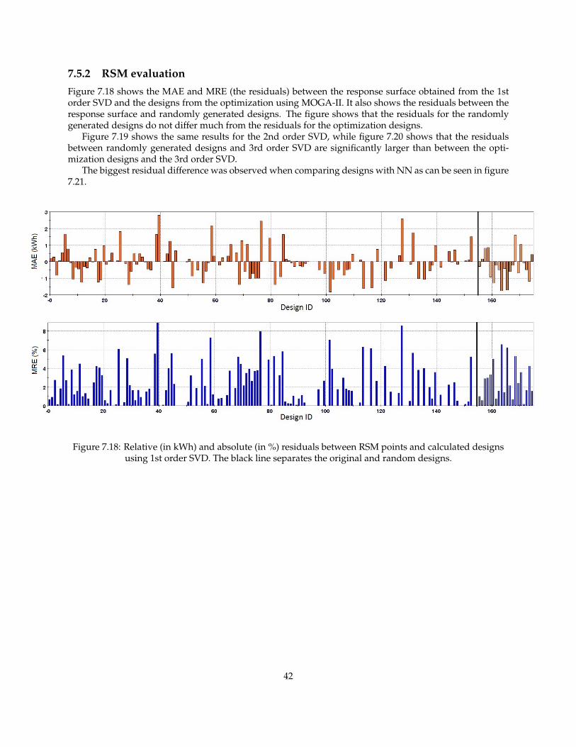
7.5.2 RSM evaluationFigure 7.18 shows the MAE and MRE (the residuals) between the response surface obtained from the 1storder SVD and the designs from the optimization using MOGA-II. It also shows the residuals between theresponse surface and randomly generated designs. The figure shows that the residuals for the randomlygenerated designs do not differ much from the residuals for the optimization designs.
Figure 7.19 shows the same results for the 2nd order SVD, while figure 7.20 shows that the residualsbetween randomly generated designs and 3rd order SVD are significantly larger than between the opti-mization designs and the 3rd order SVD.
The biggest residual difference was observed when comparing designs with NN as can be seen in figure7.21.
Figure 7.18: Relative (in kWh) and absolute (in %) residuals between RSM points and calculated designsusing 1st order SVD. The black line separates the original and random designs.
42

Figure 7.19: Relative (in kWh) and absolute (in %) residuals between RSM points and calculated designsusing 2nd order SVD. The black line separates the original and random designs.
Figure 7.20: Relative (in kWh) and absolute (in %) residuals between RSM points and calculated designsusing 3rd order SVD. The black line separates the original and random designs.
43
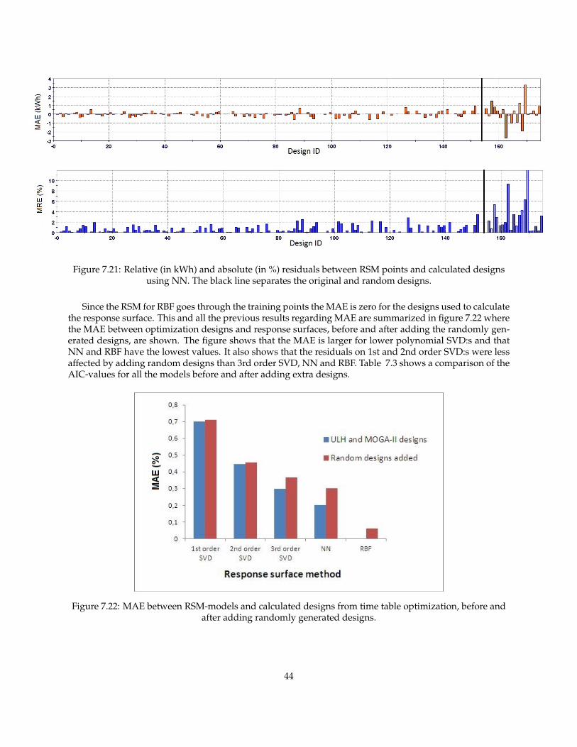
Figure 7.21: Relative (in kWh) and absolute (in %) residuals between RSM points and calculated designsusing NN. The black line separates the original and random designs.
Since the RSM for RBF goes through the training points the MAE is zero for the designs used to calculatethe response surface. This and all the previous results regarding MAE are summarized in figure 7.22 wherethe MAE between optimization designs and response surfaces, before and after adding the randomly gen-erated designs, are shown. The figure shows that the MAE is larger for lower polynomial SVD:s and thatNN and RBF have the lowest values. It also shows that the residuals on 1st and 2nd order SVD:s were lessaffected by adding random designs than 3rd order SVD, NN and RBF. Table 7.3 shows a comparison of theAIC-values for all the models before and after adding extra designs.
Figure 7.22: MAE between RSM-models and calculated designs from time table optimization, before andafter adding randomly generated designs.
44
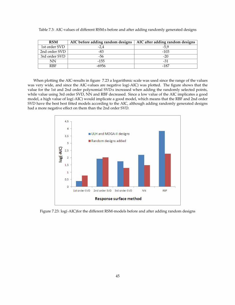
Table 7.3: AIC-values of different RSM:s before and after adding randomly generated designs
RSM AIC before adding random designs AIC after adding random designs1st order SVD -2,4 -5,92nd order SVD -83 -1033rd order SVD -56 -20
NN -155 -31RBF -6956 -187
When plotting the AIC-results in figure 7.23 a logarithmic scale was used since the range of the valueswas very wide, and since the AIC-values are negative log(-AIC) was plotted. The figure shows that thevalue for the 1st and 2nd order polynomial SVD:s increased when adding the randomly selected points,while value using 3rd order SVD, NN and RBF decreased. Since a low value of the AIC implicates a goodmodel, a high value of log(-AIC) would implicate a good model, which means that the RBF and 2nd orderSVD have the best best fitted models according to the AIC, although adding randomly generated designshad a more negative effect on them than the 2nd order SVD.
Figure 7.23: log(-AIC)for the different RSM-models before and after adding random designs
45
Discussion
8.1 Drive style comparison
A comparison between the drive style optimizer DAS and the simpler drive style AODC has been made.This comparison was partly made to cross-check the performance of DAS but also to see if a less compli-cated drive style can match the energy consumption achieved using a more complex optimizer. The drivestyle as computing using a DAS is hard to implement exactly for a driver and could only be used either asa reference or be implemented with a computer.
The results showed that the implementation of the drive styles still can be improved using DAS. Smallchanges of the input-parameters resulted in unexpected changes of the output that in some cases led tounexpected errors affecting the results. This is something already noticed by other users and will be furtherinvestigated. Furthermore the coast script did not generate the same time as the time received from TEP(rtact was not equal to rti). This was due to the slope of the speed profile calculated with the script thatdiffered from the one calculated in TEP.
When calculating the run time using coasting, the DAS-script, used to calculate coasting time, generatedan error message for many of the designs and the calculations were stopped. This happened if the train wascoasting on a part of the track where the slope was negative. This was solved by modifying the track dataso that the gradients were positive or zero on the parts where the train coasted. The comparison betweendrive styles was still possible to do and the modification did not affect the results.
The results of the comparison showed that DAS gave approximately 5 percent lower energy consump-tion than the AODC. It was also observed that the drive styles had many similarities regarding the speedprofile. By further investigating different parametrizations there is a good potential that the energy con-sumption using AODC could be decreased further. Instead of using an advanced drive style such as DAS,AODC could be used which is easy to use even for a human driver.
8.1.1 RMS-currentsWhile comparing drive styles a comparison between the RMS-currents was made. Since the RMS-currentsare correlated to the temperature in the engine it is of interest to keep them low. If one of the drive styleswould result in high RMS-currents a constraint could be of interest. The results showed that a lower energyconsumption in general resulted in lower RMS-currents, regardless of drive style. They also showed thatthe RMS-currents when using DAS in general were lower than when using AODC. The last part could beexplained by the energy consumption being lower for most of the designs using DAS. If a lower value ofthe energy consumption would have been found using coasting the RMS-current would have decreasedaccording to the trend. Early in the project adding a constraint on the RMS-currents was suggested, butsince no maximum value could be found it was chosen only to monitor the RMS-values for each design.For the results in this project a constraint would not have changed the results since the lowest energyconsumption was found where the RMS-currents were low. For future projects there is a possibility thatadding a constraint would help the optimization algorithms to search in better regions. To conclude, theRMS-currents do not restrict the values of the designs in this project.
8.2 Response surface method
In order to find the behaviour of the goal function Enet with respect to the input parameter rti differentresponse surfaces were made. The goal was to find a simple model that could describe their dependence.
46
With the help of residuals (MAE and MRE) and AIC the accuracy of the response surfaces were tested.The results showed that according to the residuals a higher order SVD, NN or RBF would give the best
approximation. Since the interpolated surface calculated by an RBF by definition always goes through thedesign points the residuals gave good results for RBF, but when randomly selected designs were added thisvalue increased drastically. By adding more points it could theoretically become higher than when usingthe other models. The results also showed that the RBF lost the least data according to the AIC, but even inthis case the value worsened when adding extra designs. To summarize, the preciseness of RBF is hard tocompare with other RSM:s due to its properties.
According to the AIC the second order SVD polynomial was the best model amongst the SVD:s, evenbetter than the NN and not far away from the RBF after adding the randomly generated designs. If morepoints had been added the second order SVD might even have become the best model according to theAIC.
The results showed that the first order SVD might be somewhat simple, two of the run times had anegative dependence of the run times which goes against the basic physics; a higher run time should givelower energy consumption. They also showed that the third order polynomial might have been affected byover-fitting, since the accuracy according to the mean square error decreased when adding extra trainingpoints. This is a typical sign of over-fitting since the accuracy for the original training point is high while itis low for the predicted data, as earlier discussed in the theory section.
To sum up, the run time dependence can be approximated with a second order polynomial, helpingfurther optimizations. It can also be concluded that it is important not to look only at one parameter whenvalidating the results.
8.3 Time table optimization of GMTD using DAS
An optimization of the run time distribution in the schedule of the a GMTD has been made. The resultshave been compared to an old schedule that was optimized by manually changing the time table in orderto find better results, called baseline.
The results can be seen as successful, but by changing the set-up it could be even more obvious that themethod has many opportunities. Firstly the baseline was already optimized various times by redistributingthe run times between stations. Secondly the optimization might have found an even better result if thescope of the project would have been wider, although according to the results Enet had almost stoppedconverging. An interesting result was that the original time table had many similarities with the optimaltime tables according to the optimization, which can give an indication that the method is working.
47

Outlook
9.1 Future time table optimization improvements
To summarize the optimization of the time table using DAS can be seen as successful, but there is still roomfor improvement. The following list gives a few examples of what can be done in future projects:
• The whole input parameter range should be regarded. By using the results from the response sur-face methods the range for the input parameters can be chosen more wisely in order to make theoptimization more efficient.
• The problems caused in DAS should be solved to avoid the unexpected errors caused by smallchanges of the input parameters.
• One restriction in this project was the script calculating the coasting point using AODC. If the opti-mizations will be done in the future, this script has to be able to handle negative gradients.
• The discarded designs can be added in order to give more information to the optimization algorithm,making the optimization faster.
• Calculations can run for a longer time in order to find an optimal time table distribution and ensurefull convergence.
• The optimization method could be tested on time tables which are not already optimized, where thereal opportunities of the method can be discovered.
• Instead of using a UHL a full-factorial DOE can be used to give a more detailed solution space.
• To find out more about the input parameter dependence it could be interesting to add more randomdesigns in the RSM:s to see what happens with the MAE and the AIC.
• Add a constraint on the RMS-currents. Since no maximum value was found within this project it wasnot added, but for those who want to take this project further and have a restriction on the RMS-currents it could easily be added.
48
Bibliography
[1] A. D’Ariano, F. Corman, I.A. Hansen, "Railway traffic optimization by advanced scheduling and rerout-ing algorithms", Delft University of Technology, Delft, The Netherlands, 2009.
[2] A. Caprara, M. Monaci, P. Toth, P. L. Guida, "A Lagrangian heuristic algorithm for a real-world traintimetabling problem", Discrete Applied Mathematics, Vol. 154, 1 April 2006, P. 738–753.
[3] K. Ghoseiri, F. Szidarovszky, M. J. Asgharpour, "A multi-objective train scheduling model and solution",Transp. Research Part B: Methodological, Vol. 38, Dec. 2004, p. 927–952.
[4] M. Larranaga, J. Anselmi, U. Ayesta, P. Jacko, A. Romo, "Optimization Techniques Applied to RailwaySystems", Basque Center for Applied Mathematics, Bilbao, Spain; Avenue du Colonel Roche, F-31400Toulouse, France, 24 Jan 2013.
[5] J. Francis, A history of the English railway: its social relations and revelations, London, England: Green andLongmans, 1851.
[6] C. Desprez, H. Djellab, "Traction energy saving by speed profile optimization". SNCF Innovation andResearch Department, 40 av. des Terroirs de France Paris 75611, France, 2012.
[7] E. Andersson, M Berg, Spårtrafiksystem och spårfordon. KTH, Avd. Spårfordon, Inst. Farkost och Flyg,Stockholm, Sweden 2007.
[8] A. A. Malikopoulos, J. P. Aguilar "Optimization of Driving Styles for Fuel Economy Improvement",Intelligent Transportation Systems, Sept. 16-19, 2012, p. 194-199.
[9] T. Guan, C. W. Frey "Model adaptive driver assistance system to increase fuel savings", Vehicular Elec-tronics and Safety, July 24-27, 2012, p. 312 - 317.
[10] V De Martinis, M Gallo "Models and methods to optimise train speed profiles with and without energyrecovery systems: a suburban test case", Procedia - Social and Behavioral Sciences, Vol. 87, 10 Oct. 2013,p. 222–233.
[11] K. Deb "Multi-Objective Optimization Using Evolutionary Algorithms: An Introduction", Departmentof Mechanical Engineering, Institute of Technology, Kanpur, India, February 2011.
[12] S. Poles, Y. Fu, E. Rigoni, "The Effect of Initial Population Sampling on the Convergence of Multi-Objective Genetic Algorithms", Multiobjective Programming and Goal Programming, Lecture Notes in Eco-nomics and Mathematical Systems Vol. 618, 2009, p. 123-133.
[13] M. D. Mckay, R. J. Beckman, W. J. Conover, "A Comparison of Three Methods for Selecting Values ofInput Variables in the Analysis of Output From a Computer Code", Technometrics, Vol. 21, No. 2, May,1979, p. 239-245.
[14] M. D. Morris, "Factorial sampling plans for preliminary computational experiments", Technometrics,Vol. 33, No. 2, May, 1991, p. 161-174.
[15] A. Karimi, P. Siarry, "Global Simplex Optimization—A simple and efficient metaheuristic for continu-ous optimization", Engineering Applications of Artificial Intelligence, Vol. 25, February 2012, p. 48–55.
[16] S. Poles, "ESTECO Technical Report 2003-005: The SIMPLEX method", ESTECO, Trieste, Italy, October7, 2003.
49
[17] U Hoffmann, Einführung in die Optimierung mit Anwendungsbeispielen aus dem Chemie-Ingenieurwesen,Germany, Verlag Chemie GMBH, 1971.
[18] A. Konak, D. W. Coit, A. Smith, "Multi-objective optimization using genetic algorithms: A tutorial inReliability Engeneering and System Safety", Information Sciences and Technology, Penn State Berks-Lehigh Valley, USA, 2006.
[19] E. Rigoni, S. Poles, "NBI and MOGA-II, two complementary algorithms for Multi-Objective optimiza-tions", ESTECO Area Science Park, Trieste, Italy, 2005.
[20] E. Rigoni, "ESTECO Technical Report 2010-004", ESTECO, Trieste, Italy, October 14, 2010.
[21] S. Razavi, B. A. Tolson, "A New Formulation for Feedforward Neural Networks", IEEE Transactionson Neural Networks, Vol. 22, no. 10, Oct. 2011.
[22] H. Akaike "A New Look at the Statistical Model Identification", IEEE Transactions on Automatic con-trol, Vol. 19, no. 6, Dec 1974, p. 716-723.
[23] I. V. Tetko, D. J. Livingstone, A. I. Luik, "Neural Network Studies. 1. Comparison of Overfitting andOvertraining", Institute of Bioorganic and Petroleum Chemistry, J. Chem. Inf. Comput. Sci., 1995, p.826–833.
[24] T. Tanneberger, "Optimization of a double decker train regarding crosswind stability", Bachelor thesis,Technische Universität, Berlin, 2012.
50