Linkoping Studies in Science and Technology.Dissertations, No. 1277

Optimization, Matroids and

Error-Correcting Codes

Martin Hessler

Division of Applied MathematicsDepartment of Mathematics

Linkoping 2009

i

ii

Optimization, Matroids and Error-Correcting Codes

Copyright c⃝ 2009 Martin Hessler, unless otherwise noted.

Matematiska institutionenLinkopings universitetSE-581 83 Linkoping, Swedenmahes@mai.liu.se

Linkoping Studies in Science and Technology.Dissertations, No. 1277

ISBN 978-91-7393-521-0ISSN 0345-7524

Printed by LiU-Tryck, Linkoping 2009

ii

iii

Abstract

The first subject we investigate in this thesis deals with optimization prob-lems on graphs. The edges are given costs defined by the values of inde-pendent exponential random variables. We show how to calculate some orall moments of the distributions of the costs of some optimization problemson graphs.

The second subject that we investigate is 1-error correcting perfectbinary codes, perfect codes for short. In most work about perfect codes, twocodes are considered equivalent if there is an isometric mapping betweenthem. We call this isometric equivalence. Another type of equivalence isgiven if two codes can be mapped on each other using a non-singular linearmap. We call this linear equivalence. A third type of equivalence is given iftwo codes can be mapped on each other using a composition of an isometricmap and a non-singular linear map. We call this extended equivalence.

∙ In Paper 1 we give a new better bound on how much the cost of thematching problem with exponential edge costs varies from its mean.

∙ In Paper 2 we calculate the expected cost of an LP-relaxed versionof the matching problem where some edges are given zero cost. Aspecial case is when the vertices with probability 1 − p have a zerocost loop, for this problem we prove that the expected cost is givenby the formula

1− 1

4+

1

9− ⋅ ⋅ ⋅ − (−p)n

n2.

∙ In Paper 3 we define the polymatroid assignment problem and give aformula for calculating all moments of its cost.

∙ In Paper 4 we present a computer enumeration of the 197 isometricequivalence classes of the perfect codes of length 31 of rank 27 andwith a kernel of dimension 24.

∙ In Paper 5 we investigate when it is possible to map two perfect codeson each other using a non-singular linear map.

∙ In Paper 6 we give an invariant for the equivalence classes of allperfect codes of all lengths when linear equivalence is considered.

∙ In Paper 7 we give an invariant for the equivalence classes of allperfect codes of all lengths when extended equivalence is considered.

∙ In Paper 8 we define a class of perfect codes that we call FRH-codes.It is shown that each FRH-code is linearly equivalent to a so calledPhelps code and that this class contains Phelps codes as a propersubset.

iii

iv

iv

v

Acknowledgements

I would like to thank my supervisor Johan Wastlund for his intuitive ex-planations of complicated concepts and for making studying mathematicsboth fun and educational. I also want to thank my second supervisor OlofHeden for his great support, for all our inspiring discussions and successfulcooperation.

This work was carried out at Linkoping University, and I would like tothank all who have given inspiring courses. I would also like to thank thedirector of postgraduate studies at Linkoping Bengt Ove Turesson.

I also would like to give many thanks to all my present and formercolleagues at the Department of Mathematics. In particular I would like tomention Jens Jonasson, Ingemar Eriksson, Daniel Ying, Gabriel Bartolini,Elina Ronnberg, Martin Ohlson, Carina Appelskog and Milagros IzquierdoBarrios.

Last but not least I would like to thank my family and friends for theirsupport and encouragement.

Linkoping, December 2009

Martin Hessler

v

vi

vi

vii

Popularvetenskaplig sammanfattning

Avhandlingen behandlar tva huvudproblem. Det forsta problemet som betraktasar hur vardet av en optimal losning for optimeringsproblem over slumpdata kanberaknas. Det andra problemet ar hur mangden av binara perfekta koder kan hit-tas och ges struktur. Bada typerna av problem har egenskapen att redan for smaproblem blir tidsatgangen for datorkorningar extremt stor. Berakningsmassigtar problemet att antalet mojliga losningar/koder vaxer extremt snabbt.

Ett optimeringsproblem som betraktas i avhandlingen ar att matcha noderi en graf. Den graf vi i allmanhet betraktar, bestar av en mangd med 2n noder,dar varje par av noder har en kant mellan sig. Vi tanker oss att varje sadan kanthar en given kostnad. En matchning i grafen ar en mangd av n kanter sadan attvarje nod har exakt en kant i matchningen. Losningen till optimeringsproblemetar den matchning som har lagst summa av kantkostnader. Antalet matchningarar storre an n! = n(n− 1) . . . 3 ⋅ 2 ⋅ 1. En naiv metod for att hitta optimum ar attberakna kostnaden for alla matchningar. Om vi tanker oss att en 4 Ghz datorkan berakna kostnaden for en matchning per klockcykel skulle det ta ca 6 gangeruniversums alder att ga igenom 27! matchningar.

For att undersoka hur optimeringsproblem beter sig pa stora grafer kan viinte betrakta alla mojliga tilldelningar av kantkostnader. Det startantagande vianvander i denna avhandling ar att vi betraktar kostnaderna som slumpmassiga.Grundtanken vi anvander illustreras ofta med Schrodingers katt. Schrodingerskatt ar tankeexperimentet att vi tanker oss en katt i en lada och innan vi oppnarladan vet vi inte om katten lever eller ar dod. I vara optimeringsproblem tankervi oss att vi betraktar en medelkant (eller en medelnod) och innan vi ”oppnarladan” vet vi varken vilken kanten ar eller hur dyr den ar.

Ett resultat ar en battre uppskattning av hur mycket vi kan forvanta oss attkostnaden for matchningen i en specifik graf avviker fran den forvantade kost-naden. Vi introducerar ocksa en generalisering av det bipartita matchningsprob-lemet. For denna generalisering ges en exakt metod for att berakna alla momentav den slumpvariabel som ger kostnaden for den generaliserade matchningen igrafen.

En perfekt kod C ar en mangd 0-1-strangar av langd n, sadan att allastrangar av langd n kan fas genom att andra pa maximalt en siffra i ett uniktelement i C. For att strukturera perfekta koder ger vi invarianter som fangarde grundlaggande egenskaperna hos koderna. En invariant ar associerad till enekvivalensrelation och har den egenskapen att alla ekvivalenta koder har sammavarde. En enkel ekvivalens ges om tva binara koder betraktas som ekvivalenta omde bara skiljer sig pa vilken ordning ettorna och nollorna star i vektorerna. Dessekvivalensklasser ar subklasser till de ekvivalensklasser som vi betraktar. Somett exempel kan vi se att C1 = {(1, 1, 0), (1, 0, 1)} och C2 = {(0, 1, 1), (1, 0, 1)}ar tva ekvivalenta koder. Dock finns det n! olika satt att ordna positionerna ikodorden i en kod, och vi vet att n! snabbt blir valdigt stort.

Ett ytterligare resultat ar att vi kan konstruera perfekta koder med varjemojlig instans av en typ av invariant. Ett foljdresultat ar att varje perfekt kodar en linjar transformation av de koder vi kan konstruera med hjalp av en av debetraktade invarianterna.

vii

viii

viii

ix

Contents

Introduction 1

1 Introduction 1

2 Graphs and optimization problems 3

3 Notation and conventions in random optimization 63.1 Exponential random variables . . . . . . . . . . . . . . . 6

4 Matroids 8

5 Optimization on a matroid 85.1 The oracle process in the general matroid setting . . . . 95.2 The minimum spanning tree (MST) problem on the com-

plete graph . . . . . . . . . . . . . . . . . . . . . . . . . 10

6 The Poisson weighted tree method 146.1 The PWIT . . . . . . . . . . . . . . . . . . . . . . . . . 146.2 The free-card matching problem . . . . . . . . . . . . . 156.3 Calculating the cost in the PWIT . . . . . . . . . . . . . 166.4 The solution to the free-card matching problem . . . . . 17

7 The main results in random optimization 19

8 Error correcting codes 21

9 Basic properties of codes 239.1 On the linear equations of a matroid . . . . . . . . . . . 24

10 The error correcting property 26

11 Binary tilings 30

12 Simplex codes 32

13 Binary perfect 1-error correcting codes 3213.1 Extended perfect codes . . . . . . . . . . . . . . . . . . . 3413.2 Equivalence and mappings of perfect codes I . . . . . . . 3413.3 The coset structure of a perfect code . . . . . . . . . . . 3613.4 Equivalences and mappings of perfect codes II . . . . . . 4013.5 The tiling representation (A,B) of a perfect code C . . 4213.6 The invariant LC . . . . . . . . . . . . . . . . . . . . . . 4413.7 The invariant L+

C . . . . . . . . . . . . . . . . . . . . . . 4713.8 The natural tiling representation of a perfect code. . . . 4913.9 Phelps codes . . . . . . . . . . . . . . . . . . . . . . . . 5113.10FRH-codes . . . . . . . . . . . . . . . . . . . . . . . . . 52

ix

x

14 Concluding remarks on perfect 1-error correcting binarycodes 52

Paper 1: Concentration of the cost of a random matchingproblem 59

M. Hessler and J. Wastlund

1 Introduction 59

2 Background and outline of our approach 60

3 The relaxed matching problem 61

4 The extended graph 62

5 A correlation inequality 64

6 The oracle process 64

7 Negative correlation 66

8 An explicit bound on the variance of Cn 68

9 Proof of Theorem 1.2 70

10 Proof of Theorem 1.3 7310.1 The distribution of a sum of independent exponentials . 7310.2 An operation on the cost matrix . . . . . . . . . . . . . 74

11 A conjecture on asymptotic normal distribution 76

Paper 2: LP-relaxed matching with free edges and loops 83M. Hessler and J. Wastlund

1 Introduction 83

2 Outline of our method 84

3 The class of telescoping zero cost flats 85

4 The zero-loop p-formula 86

5 Conclusion 92

x

xi

Paper 3: The polymatroid assignment problem 97M. Hessler and J. Wastlund

1 Introduction 97

2 Matroids and polymatroids 97

3 Polymatroid flow problems 98

4 Combinatorial properties of the polymatroid flow prob-lem 99

5 The random polymatroid flow problem 102

6 The two-dimensional urn process 103

7 The normalized limit measure 104

8 A recursive formula 105

9 The higher moments in terms of the urn process 107

10 The Fano-matroid assignment problem 108

11 The super-matching problem 110

12 The minimum edge cover 11112.1 The outer-corner conjecture and the giant component . 11512.2 The outer-corner conjecture and the two types of super-

matchings . . . . . . . . . . . . . . . . . . . . . . . . . . 117

Paper 4: A computer study of some 1-error correcting perfectbinary codes 119

M. Hessler

Introduction 121

Preliminaries and notation 122

Super dual 122

Application 123Perfect codes of length 31, rank 27 and kernel of dimension 24 . 124

xi

xii

Paper 5: Perfect codes as isomorphic spaces 135M. Hessler

Introduction 137

Preliminaries and notation 138

General results 139

Examples 140

Paper 6: On the classification of perfect codes: side class struc-tures 145

O. Heden and M. Hessler

Introduction 147

Tilings and perfect codes 152

Proof of the main theorem 153

Some classifications 158

Some remarks 161

Paper 7: On the classification of perfect codes: Extended sideclass structures 163

O. Heden, M. Hessler and T. Westerback

Introduction 165

Linear equivalence, side class structure and equivalence 167

Extended side class structure 169

More on the dual space of an extended side class structure 170

Some examples 171

Paper 8: On linear equivalence and Phelps codes 181O. Heden and M. Hessler

1 Introduction 181

xii

xiii

2 Preliminaries 1832.1 Linear equivalence and tilings . . . . . . . . . . . . . . . 1832.2 Phelps construction . . . . . . . . . . . . . . . . . . . . . 1862.3 FRH-codes . . . . . . . . . . . . . . . . . . . . . . . . . 187

3 Non full rank FRH-codes and Phelps construction 188

4 An example of a FRH-code of length 31 192

xiii

xiv

xiv

Introduction

1 Introduction

The first topic in this thesis is the research that I have done in collaborationwith Johan Wastlund, regarding how to characterize the distribution of theoptimum of some random optimization problems.

The second topic in this thesis is the work I have done in collaborationwith Olof Heden about binary 1-error correcting perfect codes. The partof the introduction about coding theory is intended to give an introductionand the main results along with more streamlined proofs than those in theoriginal Papers 4-7. Moreover this gives the opportunity to put the resultsin the proper context and clarify some general principles that were not fullydeveloped in the original articles.

We will first give two explicit examples that will exemplify the twotypes of problems we consider in this thesis. The examples are simple casesof the types of problems explored in depth later in the introduction andthe appended papers.

The first problem is an example of the type of optimization problemswe will consider, only we will later consider the costs as random.

Example 1.1. The following problem is an example of a matching prob-lem. We have four points {1, 2, 3, 4} on the real line. Suppose we want toconstruct disjoint pairs and for each pair {x, y}, x ∕= y, we have to pay∣x− y∣. We demand that every point is in exactly one pair. The optimiza-tion problem is to do this so that the sum of the costs is minimized. Clearlythe solution is to pair {1, 2} and {3, 4}.

The second problem concerns partitions of sets of binary vectors intoequivalence classes. We give a very simple example of the type of problemsthat we will consider.

Example 1.2. Consider all binary vectors of length 5 and suppose thatwe want to partition all sets of cardinality two. We may define two setsA and B as equivalent if there is a non-singular linear map µ, such that µmaps the set A on B, that is, µ(A) = B.

For any two non-zero words x and y the sets A = {0, x} and B = {0, y}there will always be a (non-unique) map µ such that A = µ(B) = {0, µ(y)}.Similarly, any two sets A = {x1, x2} and B = {y1, y2}, each consisting oftwo different non-zero vectors, will be equivalent.

1

2

Both these subjects are born out of the need to partition some finiteset in some predefined way according to a well defined criterion. In theExample 1.1, we partitioned the set {1, 2, 3, 4} in {1, 2} and {3, 4}. In theExample 1.2 we partitioned the sets of cardinality 2 into two equivalenceclasses.

When reading the mathematical descriptions, a simple picture is oftenuseful in order to structure the information presented. In this thesis Ibelieve that the picture which will facilitate understanding is a set withcertain properties that is partitioned. Another reason to try to use simplearguments is to make it easier to find counterparts with similar propertiesto the mathematical model. These counterparts give access to intuitionderived from the combined practical experience of other problems of thesame nature. Further, such a description is also helpful for people withouta background in this particular field of mathematics. Therefore we devotesome space in order to describe the general structure of the results that wewant to present in this thesis.

The main properties used here is actually closely related to simplearguments concerning dimension and linear dependencies in vector spaces.Such relations can be generalized in a number of ways. Historically a veryfamous generalization was done by H. Whitney (1935), in his article ”Onthe abstract properties of linear dependence” [32], where he introducedthe matroid concept. We will not give any details yet, these will come inSection 4.

Many real-life optimization problems can be modelled by pairwise re-lations among members of a set. Such pairwise relations are natural torepresent as a graph. Two examples closely related to this thesis are thetravelling salesman problem, TSP for short, and particle interactions.

In the parts that deal with random optimization all problems will beformulated as if the edges have some specific although random cost. Aninteresting problem in its own right is how to model specific problems withcosts on a graph. The TSP is a very natural problem in this respect. Inthe TSP the vertices in the graph represent cities and the cost of each edgeis simply the distance between the two cities. The optimization problemis to visit every city with minimal cost, that is, the shortest tour amongall the cities. In the particle interaction problem the costs are defined bythe binding energies of the atoms. The optimization problem is to formbindings, how this can be done depends upon which types of atoms we havein the system, in such a way that the total energy is minimized.

In the random optimization problems studied in the attached papers,each edge in a graph is given a random cost. One of the results is a betterbound on how much the cost of the matching problem varies from the mean.We calculate the mean and higher moments of some previously unsolvedgeneralizations of the matching problem.

In coding theory the corresponding real-life problem, is how to com-municate information. That is, if we say something to someone we want

2

3

to be reasonably sure that the person we are talking to understands whatwe say. Observe that even if we assume that two persons speak the samelanguage there might be communication problems in between them. Oneway to think of this is how easily words can be misheard if they closely re-semble each other. The conclusion is that we do not want words to be toosimilar. As an example, consider draft and graft, these words only differin one position and each of these words could easily be mistaken for theother. Luckily their meanings are such that most of the time the contextwill clarify which is the correct interpretation. But a misunderstandingwould be most unfortunate if we are communication with the authorities.In a mathematical context this can be thought of as a partitioning problem.The problem is how to partition all sequences of letters in such a way thatall small changes of the words result in something that is not a word. Butthis should be done in an efficient way so that we do not get unnecessarilylong words in our language.

In coding theory we give a different approach to how to structurethe, so called, perfect codes. This new structure gives new tools how toenumerate, classify and relate different classes of perfect codes. We givenew invariants for some equivalence relations on the set of perfect codes.We also give a non-trivial result on how a certain class of perfect codes, thePhelps codes, is related to an equivalence relation on the family of perfectcodes.

This study of perfect codes has been motivated by a need to find a newapproach that can overcome the problems inherited by the large number ofdifferent representations in each equivalence class of perfect codes.

2 Graphs and optimization problems

We consider a graph as a pair of sets (V,E), the set V = {vi} for i = 1 . . . n,is some numbering of the vertices in the graph and the set E denotes theedges. The degree of a vertex vi in a graph is the number of edges eij ∈ E.We will also in some cases refer to the degree of a vertex in some sub-graph,(V, F ) for F ⊂ E, where it is defined in the natural way.

We will here always consider the case that we have undirected edges,that is, for every edge eij ∈ E, eij = eji. This is natural in the travel-ling salesman problem if we consider the costs of the edges as distances.But if we consider the costs as ticket prices, we don’t necessary have thissymmetry.

A loop in a graph is an edge eii whose endpoints coincide. If weconsider graphs with loops we will state this explicitly, that is, the defaultcase is a graph without loops.

A graph is complete if there exists an edge eij for every pair i, j ∈ [1, n],such that i ∕= j.

A bipartite graph is a graph where we can split the vertex set V intotwo disjoint sets A and B such that every edge in E goes between a vertex

3

4

in A and a vertex in B. A complete bipartite graph is a bipartite graphsuch that for every pair vi ∈ A and vj ∈ B there exists an edge eij .

A forest is a graph without cycles. In a connected graph there isa path connecting any pair of vertices. A tree is a forest such that thesubgraph, defined by the vertices having an edge in the forest, is connected.A spanning tree is a tree that contains every vertex of the graph. Hencethere is a unique path connecting any two vertices in a spanning tree.

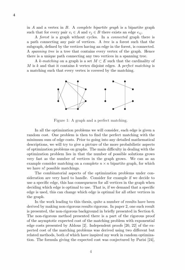
A k-matching on a graph is a set M ⊂ E such that the cardinality ofM is k and that it contains k vertex disjoint edges. A perfect matching isa matching such that every vertex is covered by the matching.

Figure 1: A graph and a perfect matching.

In all the optimization problems we will consider, each edge is given arandom cost. One problem is then to find the perfect matching with theminimum sum of edge costs. Prior to going into any detailed mathematicaldescriptions, we will try to give a picture of the more probabilistic aspectsof optimization problems on graphs. The main difficulty in dealing with theoptimization problem lies in that the number of possible solutions growsvery fast as the number of vertices in the graph grows. We can as anexample consider matching on a complete n× n bipartite graph, for whichwe have n! possible matchings.

The combinatorial aspects of the optimization problems under con-sideration are very hard to handle. Consider for example if we decide touse a specific edge, this has consequences for all vertices in the graph whendeciding which edge is optimal to use. That is, if we demand that a specificedge is used, this can change which edge is optimal for all other vertices inthe graph.

In the work leading to this thesis, quite a number of results have beenderived by making non-rigorous results rigorous. In paper 2, one such resultis presented, the non-rigorous background in briefly presented in Section 6.The non-rigorous method presented there is a part of the rigorous proofof the asymptotic expected cost of the matching problem with exponentialedge costs presented by Aldous [2]. Independent proofs [20, 22] of the ex-pected cost of the matching problems was derived using two different butrelated methods, both of which have inspired my work in random optimiza-tion. The formula giving the expected cost was conjectured by Parisi [24],

4

5

this formula gives the expected cost on the complete bipartite graph withn+ n vertices as

1 +1

4+

1

9+ ⋅ ⋅ ⋅+ 1

n2→ ¼2

6.

The method we use to solve problems in random optimization in thisthesis involves constructing something very much like an algorithm. Thisalgorithm recursively finds the optimum solution, i.e. we first find the opti-mum 1-matching and then use the information gained to find the optimum2-matching and so forth. Constructing such an algorithm mainly deals withhow to acquire information about the edge costs while maintaining somenice probabilistic properties of the random variables involved. We will nowconsider some examples of how choosing the right way to condition on therandom variables can help us answer questions about random structures.

Example 2.1. Suppose that we have two dice with six sides, one blue,one red. Consider first that we condition on the event that at least one dieis equal to two. What is the probability that both dice are equal to two?What if we instead condition on the event that the blue die is equal to two?In the first case the probability is 1/11 and in the second case 1/6.

Example 2.2. Suppose that we have a thousand dice with six sides. Whatis the probability that the sum is divisible by six? What happens if wecondition on that the sum of the first 999 dice is equal to n? The probabilityis 1/6.

Example 2.3. Suppose we place 3 points independently randomly withuniform distribution on a circle. What is the probability that we can rotatethe circle in such a way that all points lie on the right hand side of the circle?One solution is to condition on the lines that we get through the centre ofthe circle and the 3 points, but not on which side of the origin the pointslie. In principle there are only 6 ways to rotate the circle in order to getthe points on the right side. Further there are 8 ways to choose which sideof origin the points lie. Hence the probability is 3/4.

A fundamental property to maintain (or prove), is that the randomvariables are independent. It is easy to see that in the travelling salesmanproblem with costs given by distances between points, it is not even possibleto start with independent costs. As the edge costs must pointwise in theprobability space (every arrangement of the vertices in the plane) fulfil thetriangle inequality. Clearly the triangle inequality leads to a dependency forthe cost random variables. To get a manageable problem we define a relatedproblem where we assume that the random variables are independent. Fromthis approach a large class of interesting problems has evolved, some ofwhich are considered in the papers in this thesis.

In paper 1 we use an exact method to get a bound on how much thecost varies from the average cost for the matching problem.

5

6

In paper 2 we derive a formula for the expected cost of a specificgeneralization of the matching problem.

In paper 3 we give a generalization of the bipartite matching problemwhere we allow more intricate restrictions on each of the two sets of vertices.For this problem we give an exact formula for all moments.

When we construct the methods used in this thesis, the most impor-tant statements involve how different partial solutions are related to eachother. Whitney defined the class of matroids in his famous paper [32]. Foran optimization problem on a matroid, it is possible to make statementsabout how partial solutions are related. In fact, matroids have a s strongerproperty than we need, the property that we can find the optimal solutionusing a greedy algorithm. But for the purpose of this thesis we will usea language suitable for a larger class of optimization problems, to whichfor example the assignment problem belongs. We will devote Section 4 togive a short description of matroids. Although of limited practical use,we believe that the matroid example is very informative in relation to ourpapers about random optimization.

3 Notation and conventions in random opti-mization

In this section, we specify the notation and definitions needed for our studyof some random optimization problems.

3.1 Exponential random variables

Many of the methods used in this thesis are completely dependent on spe-cific properties of exponential random variables. An exponential randomvariable X of rate ° > 0 is a random variable with the density functionfX(x) = ° exp(−°x). We get the probability

P (X ≤ x) =

∫ x

0

fX(t)dt.

We define FX(x) = P (X ≤ x) and FX(x) = P (X > x) = 1 − FX(x).Hence, FX(x) is the probability function (the distribution) of the randomvariable X. We list some of the properties of exponential random variablesbelow, we include short proofs of these properties.

Lemma 3.1. (The memorylessness property)Let X be an exponential random variable of rate °. Conditioned on theevent that X is larger than some constant k, the increment size X − k isan exponential random variable Xk of rate °, in other words,

P (X > k + t∣X > k) = P (X > t). (1)

6

7

Proof. We only need to note that

P (X > k) = exp(−°k),

and

exp(°k) exp(−°(x+ k) = exp(−°x).

Lemma 3.2. For any set {X1, . . . , Xn} of independent exponential randomvariables Xi of rates °i, Z = min(X1, . . . , Xn) is a rate ° = °1+°2+⋅ ⋅ ⋅+°nexponential random variable.

Proof. P (Z > x) = exp(−°1x) ⋅ ⋅ ⋅ ⋅ ⋅ exp(−°nx) = exp(−°x)

Lemma 3.3. (The index of the minimum)For any set {X1, . . . , Xn} of independent exponential random variables Xi

of rates °i and the minimum Z = min(X1, . . . , Xn). Then Xj = Z withprobability

°j°1 + ⋅ ⋅ ⋅+ °n

.

Proof. Assume without loss of generality that j = 1. By Lemma 3.2, therandom variable Y = min(X2, . . . , Xn) is exponential of rate °2 + ⋅ ⋅ ⋅+ °n,it follows that

P (X1 = Z) = P (X1 < Y ) =

∫ ∞

0

fX1(x)FY (x)dx =°1

°1 + ⋅ ⋅ ⋅+ °n.

Lemma 3.4. (The independence property of the value and theindex of the minimum of a set)For any set {X1, . . . , Xn} of independent exponential random variables Xi

of rates °i and the minimum Z = min(X1, . . . , Xn). Let I be the randomvariable such that XI = Z. Then Z and I are independent.

Proof. Again assume that j = 1 and define the random variable Y =min(X2, . . . , Xn). With this terminology we get

P (I = 1, Z > x) = P (Y > X1 > x) =

∫ ∞

x

fX1(t)FY (t)dt =

°1 exp(−x(°1 + °1))

°1 + °2= P (I = 1)P (Z > x).

7

8

4 Matroids

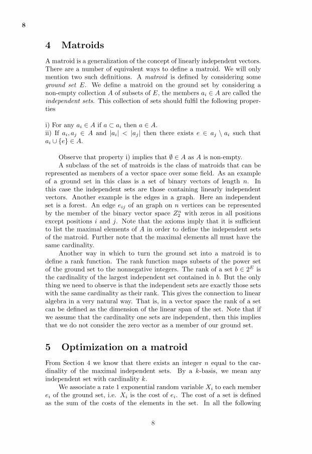
A matroid is a generalization of the concept of linearly independent vectors.There are a number of equivalent ways to define a matroid. We will onlymention two such definitions. A matroid is defined by considering someground set E. We define a matroid on the ground set by considering anon-empty collection A of subsets of E, the members ai ∈ A are called theindependent sets. This collection of sets should fulfil the following proper-ties

i) For any ai ∈ A if a ⊂ ai then a ∈ A.ii) If ai, aj ∈ A and ∣ai∣ < ∣aj ∣ then there exists e ∈ aj ∖ ai such thatai ∪ {e} ∈ A.

Observe that property i) implies that ∅ ∈ A as A is non-empty.A subclass of the set of matroids is the class of matroids that can be

represented as members of a vector space over some field. As an exampleof a ground set in this class is a set of binary vectors of length n. Inthis case the independent sets are those containing linearly independentvectors. Another example is the edges in a graph. Here an independentset is a forest. An edge eij of an graph on n vertices can be representedby the member of the binary vector space Zn

2 with zeros in all positionsexcept positions i and j. Note that the axioms imply that it is sufficientto list the maximal elements of A in order to define the independent setsof the matroid. Further note that the maximal elements all must have thesame cardinality.

Another way in which to turn the ground set into a matroid is todefine a rank function. The rank function maps subsets of the power setof the ground set to the nonnegative integers. The rank of a set b ∈ 2E isthe cardinality of the largest independent set contained in b. But the onlything we need to observe is that the independent sets are exactly those setswith the same cardinality as their rank. This gives the connection to linearalgebra in a very natural way. That is, in a vector space the rank of a setcan be defined as the dimension of the linear span of the set. Note that ifwe assume that the cardinality one sets are independent, then this impliesthat we do not consider the zero vector as a member of our ground set.

5 Optimization on a matroid

From Section 4 we know that there exists an integer n equal to the car-dinality of the maximal independent sets. By a k-basis, we mean anyindependent set with cardinality k.

We associate a rate 1 exponential random variable Xi to each memberei of the ground set, i.e. Xi is the cost of ei. The cost of a set is definedas the sum of the costs of the elements in the set. In all the following

8

9

discussions we will assume that no two subsets have the same cost. Thisproperty makes it possible to use the notation that amin

k ∈ A is the uniqueminimum cost k-basis.

Lemma 5.1. (The nesting property)If k1 < k2 then amin

k1⊂ amin

k2.

Proof. By matroid property i) and the minimality of amink1

every subset

of cardinality k1 of amink2

is a k1-basis of equal or higher cost than amink1

.

By matroid property ii) there is a subset a of amink2

such that a ∪ amink1

is

a k2-basis. The minimality and uniqueness of amink2

implies that amink2

=

a ∪ amink1

.

We define the span of a set a as the largest set containing a with thesame rank as a.

5.1 The oracle process in the general matroid setting

An oracle process is a systematic way to structure information in an opti-mization process. We assume that there is an oracle who knows everythingabout the costs of the elements of the ground set.

We now give a protocol for how we ask questions to the oracle in thematroid setting with exponential rate 1 variables. The protocol is formu-lated as a list of information which we are in possession of when we knowthe minimal k-basis.

1) We know the set amink , this implies that we know the set span(amin

k ).2) We know the cost of all the random variables associated to the setspan(amin

k ).3) We know the minimum of all the exponential random variables associ-ated to the elements ei in the set E ∖ span(amin

k ).

Here we then conclude that we know exactly the information needed inorder to know the cost of the minimal k + 1-basis. To know the stipulatedinformation in the next step of the optimization process we need to askthe oracle two questions. First we ask which member of the ground setis associated to the minimum under bullet 3). Second we ask about allthe missing costs under bullet 2) and 3). Now we have reached the pointwhere we run into problems with the combinatorial structure of a particularproblem. That is when we ask for the cost of the minimum under bullet(3) the expected value of this is just

1

∣E ∖ span(amink )∣ , (2)

larger than the value we got the last time we asked for this cost. The prob-lem is that the cardinality depend on which set amin

k we have. Therefore we

9

10

need to know the properties of these sets. The independence of the mini-mum and its location often enables us to calculate the expected cardinalityof the above set.

By the construction of the questions 1)-3) to the oracle we controlexactly which information we are in possession of at any time. We be-lieve that constructing a good protocol is the key to solving optimizationproblems possessing the nesting property.

Note that only a few problems can be formulated directly as an opti-mization problem on the ground set of a matroid. Most of the times weneed to use some generalization of the matroid. But such generalizationsseem to possess similar properties to the ones used above. Further theintuition given by the basic matroid formulation seems to generalize in anatural way. An additional motivation is that we will in some of the moreadvanced problems, see Paper 3, in this thesis need to calculate the waitingtimes in a two-dimensional urn-process. These waiting times correspond tohow much larger the next random variable we ask for in bullet 3).

5.2 The minimum spanning tree (MST) problem onthe complete graph

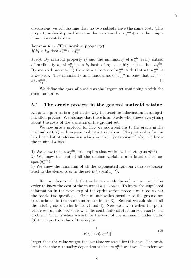
In terms of graphs the most natural matroid structure, where we have adirect correspondence between the edges and the ground set, is the spanningtrees of a graph. In this setting a maximal independent set is the set ofedges from a spanning tree. The asymptotic cost ³(3) of the MST was firstcalculated by Frieze [6]. We observed above that calculating Equation (2)is the main difficulty in the oracle process. In this example we will showhow we here can calculate the number ∣E ∖ span(aj)∣P (amin

k = aj) for all jand k.

We start by looking at two small examples where it is reasonable todo the complete calculations needed to get the expected value of the mini-mum spanning tree. We denote the random variable giving the cost of theminimum k-basis on a complete graph by Tn

k .For n = 3 the complete graph has 3 edges, as can be seen in Figure 2.

Observe, in this example, that the matroid structure does not restrict uswhen we choose edges for the 2-basis. We can choose the two smallest edgesand get the result directly. By symmetry assume thatX1 < X2 < X3 givingthe result

ET 32 = E(min(X1 +X2, X1 +X3, X2 +X3)) = (3)

E(X1 +X2∣X1 < X2 < X3) = 1/3 + (1/3 + 1/2) = 7/6. (4)

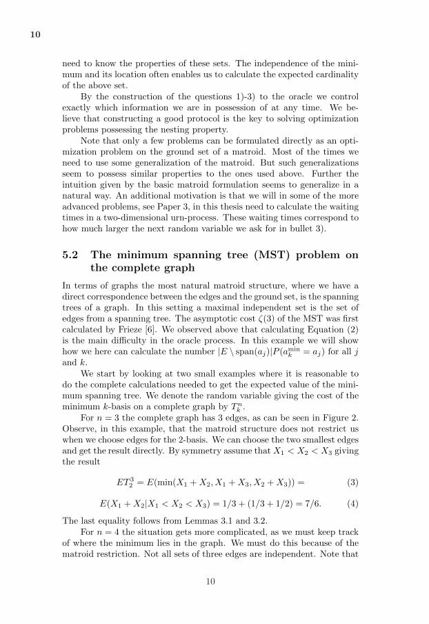
The last equality follows from Lemmas 3.1 and 3.2.For n = 4 the situation gets more complicated, as we must keep track

of where the minimum lies in the graph. We must do this because of thematroid restriction. Not all sets of three edges are independent. Note that

10

11

v1 v2

v3

v1 v2

v3v4

Figure 2: The complete graphs K3 and K4.

Figure 3: The two types of spanning trees in K4.

11

12

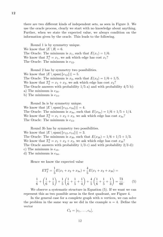
there are two different kinds of independent sets, as seen in Figure 3. Weuse the oracle process, clearly we start with no knowledge about anything.Further, when we state the expected value, we always condition on theinformation given by the oracle. This leads to the following.

Round 1 is by symmetry unique.We know that ∣E ∖ ∅∣ = 6.The Oracle: The minimum is x1, such that E(x1) = 1/6.We know that T 4

1 = x1, we ask which edge has cost x1?The Oracle: The minimum is e12.

Round 2 has by symmetry two possibilities.We know that ∣E ∖ span({e12})∣ = 5.The Oracle: The minimum is x2, such that E(x2) = 1/6 + 1/5.We know that T 4

2 = x1 + x2, we ask which edge has cost x2?The Oracle answers with probability 1/5 a) and with probability 4/5 b):a) The minimum is e34.b) The minimum is e14.

Round 3a is by symmetry unique.We know that ∣E ∖ span({e12, e34})∣ = 4.The Oracle: The minimum is x3a, such that E(x3a) = 1/6 + 1/5 + 1/4.We know that T 4

3 = x1 + x2 + x3, we ask which edge has cost x3a?The Oracle: The minimum is e13.

Round 3b has by symmetry two possibilities.We know that ∣E ∖ span({e12, e14})∣ = 3.The Oracle: The minimum is x3b, such that E(x3b) = 1/6 + 1/5 + 1/3.We know that T 4

3 = x1 + x2 + x3, we ask which edge has cost x3b?The Oracle answers with probability 1/3 c) and with probability 2/3 d):c) The minimum is e13.d) The minimum is e34.

Hence we know the expected value

ET 43 =

1

5E(x1 + x2 + x3a) +

4

5E(x1 + x2 + x3b) =

1

6+

(1

6+

1

5

)+

1

5

(1

6+

1

5+

1

4

)+

4

5

(1

6+

1

5+

1

3

)=

73

60. (5)

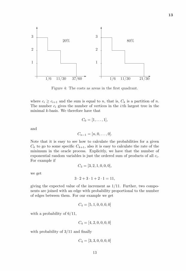
We observe a systematic structure in Equation (5). If we want we canrepresent this as two possible areas in the first quadrant, see Figure 4.

In the general case for a complete graph with n vertices, we can solvethe problem in the same way as we did in the example n = 4. Define thevector

Ck = [c1, . . . , cn],

12

13

6

-1/6 11/30 37/60

1

2

320%

6

-1/6 11/30 21/30

1

2

380%

Figure 4: The costs as areas in the first quadrant.

where ci ≥ ci+1 and the sum is equal to n, that is, Ck is a partition of n.The number ci gives the number of vertices in the i:th largest tree in theminimal k-basis. We therefore have that

C0 = [1, . . . , 1],

and

Cn−1 = [n, 0, . . . , 0].

Note that it is easy to see how to calculate the probabilities for a givenCk to go to some specific Ck+1, also it is easy to calculate the rate of theminimum in the oracle process. Explicitly, we have that the number ofexponential random variables is just the ordered sum of products of all ci.For example if

C3 = [3, 2, 1, 0, 0, 0],

we get

3 ⋅ 2 + 3 ⋅ 1 + 2 ⋅ 1 = 11,

giving the expected value of the increment as 1/11. Further, two compo-nents are joined with an edge with probability proportional to the numberof edges between them. For our example we get

C4 = [5, 1, 0, 0, 0, 0]

with a probability of 6/11,

C4 = [4, 2, 0, 0, 0, 0]

with probability of 3/11 and finally

C4 = [3, 3, 0, 0, 0, 0]

13

14

with a probability of 2/11. We observe that we only need to do the sum-mation over all such states to get the expected cost of the MST, but thisis time consuming to do on a computer even for moderately large n. As anexample see Gamarnik [7], for a different and more efficient algorithm howto do this on a computer.

6 The Poisson weighted tree method

In this section we describe a non-rigorous method for computing the costof a matching on the complete graph.

In the normal matching problem every vertex must be matched. Wehere study a related problem where we for each vertex with a coin flip decideif the vertex must be matched with a probability p (p = 1 corresponds tothe normal matching problem). We call this problem the free-card match-ing problem as we can think of the vertices that do not need to be in thematching as having a card that allows them to be exempt from the match-ing. The free-card matching problem is asymptotically equivalent (in termsof expected cost) to the problem studied in Paper 2.

Results based on the Poisson weighted infinite tree, PWIT for short,have been made rigorous in some cases. In [2] it was used to prove the ¼2/6limit of the bipartite matching problem. Aldous also gave non-rigorousarguments to motivated the calculations used in [2]. We generalize thesenon-rigorous arguments in order to get a model suitable for the free-cardmatching problem.

In the previous sections we have considered finite graphs, we hereconsider the limit object of a complete graph Kn, when we let the numberof vertices grow. Hence in all further discussions we will regard n as large.

6.1 The PWIT

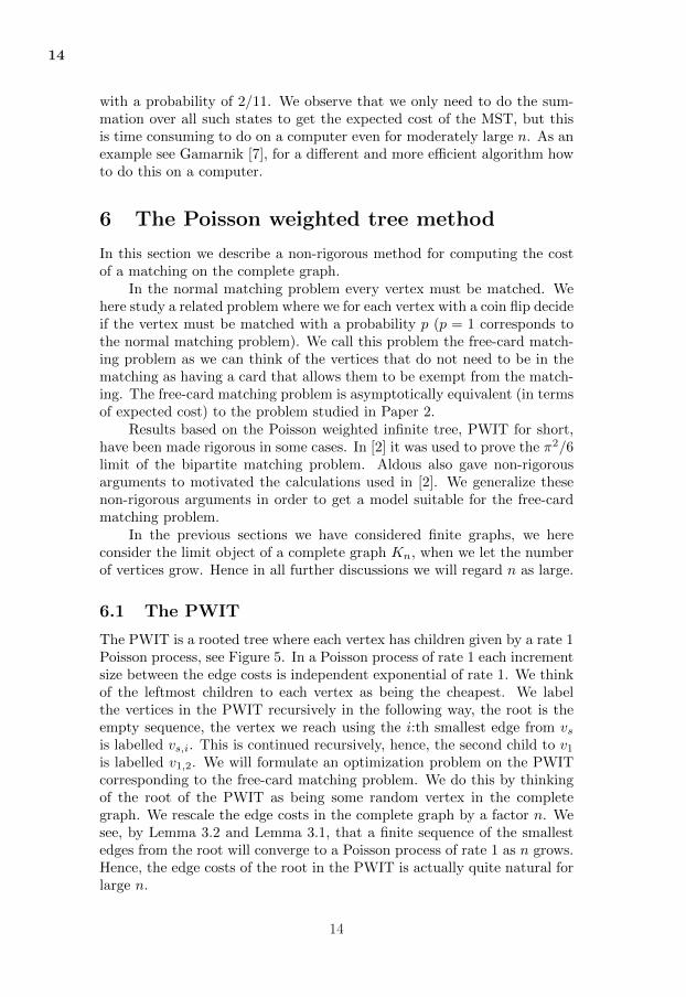
The PWIT is a rooted tree where each vertex has children given by a rate 1Poisson process, see Figure 5. In a Poisson process of rate 1 each incrementsize between the edge costs is independent exponential of rate 1. We thinkof the leftmost children to each vertex as being the cheapest. We labelthe vertices in the PWIT recursively in the following way, the root is theempty sequence, the vertex we reach using the i:th smallest edge from vsis labelled vs,i. This is continued recursively, hence, the second child to v1is labelled v1,2. We will formulate an optimization problem on the PWITcorresponding to the free-card matching problem. We do this by thinkingof the root of the PWIT as being some random vertex in the completegraph. We rescale the edge costs in the complete graph by a factor n. Wesee, by Lemma 3.2 and Lemma 3.1, that a finite sequence of the smallestedges from the root will converge to a Poisson process of rate 1 as n grows.Hence, the edge costs of the root in the PWIT is actually quite natural forlarge n.

14

15

Z

Z1 Z2 Z3

»1 »2 »3

Figure 5: The Poisson weighted infinite tree.

6.2 The free-card matching problem

Let p be any number such that 0 ≤ p ≤ 1 and consider a complete graphKn with independent exponential rate 1 edge costs. To each vertex weindependently give a free-card with probability 1 − p. The optimizationproblem is to find the set of vertex disjoint edges with minimal cost thatcovers every vertex without a free-card. We denote the random variablegiving the cost of the optimal free-card matching by Fn, for even n. Thecost is expressed in the dilog-function, this function is defined by

dilog(t) =

∫ t

1

log(x)

1− xdx.

For the free-card matching problem we want to prove, within the framworkof the PWIT-method, the following:

Conjecture 6.1. Let Fn be the cost of the optimal free-card matching, then

EFn −→ −dilog(1 + p).

In the PWIT we model the free-card matching problem by choosinga free-card matching on the PWIT. As above, each vertex is given a free-card independently with probability 1− p. We note that a vertex is eithermatched to its parent or it is used in the free-card matching in its subtree.We assume that we, by the above mentioned renormalization, have welldefined random variables Zv for each vertex v in the PWIT. These randomvariables give the difference in cost between the minimal free-card matching

15

16

in the subtree to v where we use the root in the free-card matching and thefree-card matching that does not use the root. We assume that each Zv isonly dependent on the random variables in the subtree with v as root. Wefurther assume that all Zv have the same distribution.

We describe the minimality condition on the free-card matching by asystem of “recursive distributional equations”. Recall that when we ran-domly pick the root, it either owns a free-card or it does not own a free-card.Denote the distribution of Zv conditioning on v getting a free card by Yv

and conditioning on that v do not get a free card by Xv. We describe therelation between the random variables with the following system

{X

d= min (»i −Xi; ³i − Yi) ,

Yd= min (0; »i −Xi; ³i − Yi) .

(6)

Here » is a Poisson process of rate p and ³ is a Poisson process of rate1 − p. This follows by the splitting property of a Poisson process. Thelogic of the system is that, when we match the root, we do this in such away that we minimize the cost of the free-card matching problem on thePWIT. Further, if we match the root to a specific child, the child is nolonger matched in its sub-tree.

6.3 Calculating the cost in the PWIT

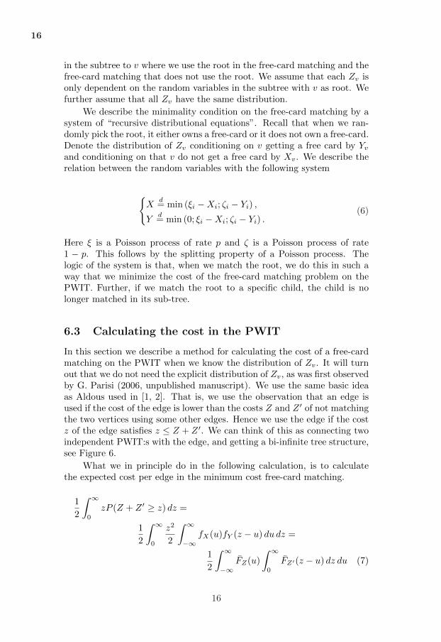
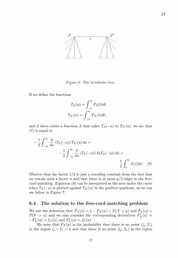
In this section we describe a method for calculating the cost of a free-cardmatching on the PWIT when we know the distribution of Zv. It will turnout that we do not need the explicit distribution of Zv, as was first observedby G. Parisi (2006, unpublished manuscript). We use the same basic ideaas Aldous used in [1, 2]. That is, we use the observation that an edge isused if the cost of the edge is lower than the costs Z and Z ′ of not matchingthe two vertices using some other edges. Hence we use the edge if the costz of the edge satisfies z ≤ Z + Z ′. We can think of this as connecting twoindependent PWIT:s with the edge, and getting a bi-infinite tree structure,see Figure 6.

What we in principle do in the following calculation, is to calculatethe expected cost per edge in the minimum cost free-card matching.

1

2

∫ ∞

0

zP (Z + Z ′ ≥ z) dz =

1

2

∫ ∞

0

z2

2

∫ ∞

−∞fX(u)fY (z − u) du dz =

1

2

∫ ∞

−∞FZ(u)

∫ ∞

0

FZ′(z − u) dz du (7)

16

17

Z Z ′z

Figure 6: The bi-infinite tree.

If we define the functions

TZ(u) =

∫ ∞

−u

FZ(t)dt

TZ′(u) =

∫ ∞

−u

FZ′(t)dt,

and if there exists a function Λ that takes TZ(−u) to TZ′(u), we see that(7) is equal to

− 1

2

∫ ∞

−∞

d

du(TZ(−u))TZ′(u) du =

− 1

2

∫ ∞

−∞

d

du(TZ(−u)) Λ(TZ(−u)) du =

1

2

∫ ∞

0

Λ(x)dx. (8)

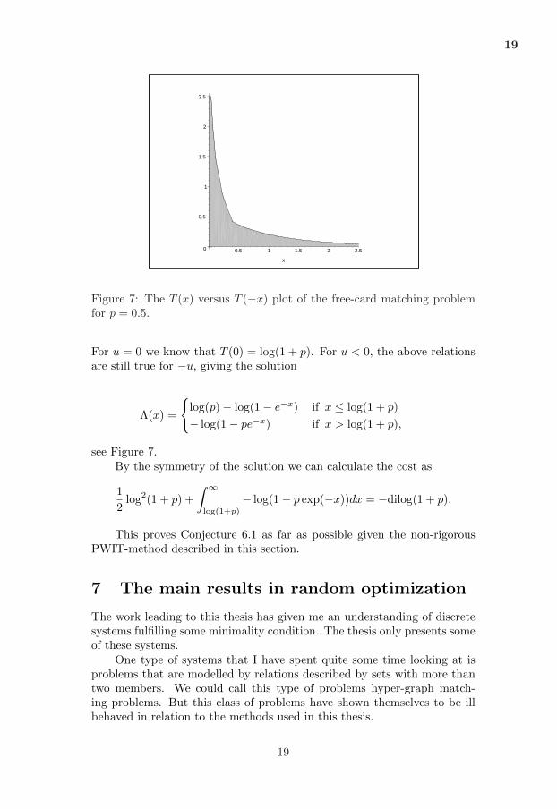
Observe that the factor 1/2 is just a rescaling constant from the fact thatwe rescale with a factor n and that there is at most n/2 edges in the free-card matching. Equation (8) can be interpreted as the area under the curvewhen TZ(−u) is plotted against TZ′(u) in the positive quadrant, as we cansee below in Figure 7.

6.4 The solution to the free-card matching problem

We use the definition that FX(u) = 1 − FX(u) = P (X > u) and FY (u) =P (Y > u) and we also consider the corresponding derivatives F ′

X(u) =−F ′

X(u) = fX(u) and F ′Y (u) = fY (u).

We note that FX(u) is the probability that there is no point (³i, Yi)in the region ³i − Yi < u and that there is no point (»i, Xi) in the region

17

18

»i −Xi < u. We get

FX(u) = exp

(−∫ ∞

−u

pFX(t) + (1− p)FY (t)dt

),

and similarly for FY (u).With this observation we see that the system (6) corresponds to

fX(u) = pFX(u)FX(−u) + (1− p)FX(u)FY (−u) (9)

FY (u) =

{0 if u > 0

FX(u) if u < 0.

It follows that

fX(u) =

{pFX(u)FX(−u) if u < 0

FX(u)FX(−u) if u > 0.

This system implies that pfX(u) = fX(−u) if u > 0 and moreover thatpFX(u) = FX(−u). Using this we can solve (9) and get that

FX(u) = 1− 1

p+ eu+cif u > 0.

The constant c follows from the fact that FX(0−)+ FX(0+) = 1 whichgive that c = 0. We also get the probability

P (Y = 0) = FY (0−) = 1− pFX(0+) = (1− p)/(1 + p).

Collecting the above results give that

FX(u) = Â(−∞,0)(u)

(p

p+ e−u

)+ Â[0,∞)(u)

(1− 1

p+ eu

)(10)

FY (u) = Â(−∞,0)(u)

(p

p+ e−u

)+ Â[0,∞)(u).

In order to calculate the expected cost we use Equation (8). We define

T (u) =

∫ ∞

−u

pFX(s) + (1− p)FY (s) ds.

Note that we consider a random choice of root in this expression. ByEquation (10) we see that for u > 0 we get that FX(−u) + pFX(u) = p,which together with the relation FX(u) = exp(−T (u)) implies that

e−T (−u) + pe−T (u) = 1.

18

19

0

0.5

1

1.5

2

2.5

0.5 1 1.5 2 2.5

x

Figure 7: The T (x) versus T (−x) plot of the free-card matching problemfor p = 0.5.

For u = 0 we know that T (0) = log(1 + p). For u < 0, the above relationsare still true for −u, giving the solution

Λ(x) =

{log(p)− log(1− e−x) if x ≤ log(1 + p)

− log(1− pe−x) if x > log(1 + p),

see Figure 7.By the symmetry of the solution we can calculate the cost as

1

2log2(1 + p) +

∫ ∞

log(1+p)

− log(1− p exp(−x))dx = −dilog(1 + p).

This proves Conjecture 6.1 as far as possible given the non-rigorousPWIT-method described in this section.

7 The main results in random optimization

The work leading to this thesis has given me an understanding of discretesystems fulfilling some minimality condition. The thesis only presents someof these systems.

One type of systems that I have spent quite some time looking at isproblems that are modelled by relations described by sets with more thantwo members. We could call this type of problems hyper-graph match-ing problems. But this class of problems have shown themselves to be illbehaved in relation to the methods used in this thesis.

19

20

The intention has been to communicate some of my understanding tomore people. Further, it is possible to derive the results in the papers fromwell known results from calculus, often in the form of partial integrationor by changing the order of integration. This is the method I have mostlyused to derive the results. The reader should be aware of this as it is notalways clear from the composition of the papers. The presentation in thepapers is chosen with consideration to how easy it will be to generalize theresults, but also to put the results into a familiar framework to the typicalreader.

As a final remark we want to again note that perhaps the most im-portant result in the papers is that they give further indications how toapproach similar problems in the future. They give additional evidencethat the methods used are well suited for giving strong results. The lastpaper, gives an even more general interpretation of a 2-dimensional urnprocess, this gives additional tools to find a combinatorial interpretationof this method. Further it seems that approximating the higher momentsusing the method in Paper 1, give better bounds than those attainable withother methods.

20

21

8 Error correcting codes

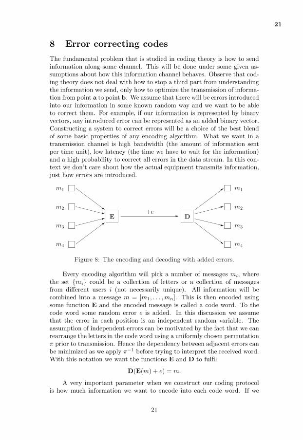
The fundamental problem that is studied in coding theory is how to sendinformation along some channel. This will be done under some given as-sumptions about how this information channel behaves. Observe that cod-ing theory does not deal with how to stop a third part from understandingthe information we send, only how to optimize the transmission of informa-tion from point a to point b. We assume that there will be errors introducedinto our information in some known random way and we want to be ableto correct them. For example, if our information is represented by binaryvectors, any introduced error can be represented as an added binary vector.Constructing a system to correct errors will be a choice of the best blendof some basic properties of any encoding algorithm. What we want in atransmission channel is high bandwidth (the amount of information sentper time unit), low latency (the time we have to wait for the information)and a high probability to correct all errors in the data stream. In this con-text we don’t care about how the actual equipment transmits information,just how errors are introduced.

-~z:>

>

:

z

~

+eE D

m4

m3

m2

m1

m4

m3

m2

m1

Figure 8: The encoding and decoding with added errors.

Every encoding algorithm will pick a number of messages mi, wherethe set {mi} could be a collection of letters or a collection of messagesfrom different users i (not necessarily unique). All information will becombined into a message m = [m1, . . . ,mn]. This is then encoded usingsome function E and the encoded message is called a code word. To thecode word some random error e is added. In this discussion we assumethat the error in each position is an independent random variable. Theassumption of independent errors can be motivated by the fact that we canrearrange the letters in the code word using a uniformly chosen permutation¼ prior to transmission. Hence the dependency between adjacent errors canbe minimized as we apply ¼−1 before trying to interpret the received word.With this notation we want the functions E and D to fulfil

D(E(m) + e) = m.

A very important parameter when we construct our coding protocolis how much information we want to encode into each code word. If we

21

22

make the code words long we have better control of how many errors eachcode word can contain. Consider for example code words of length 1. Sucha word will either be correct or incorrect. However, if the code words arelong, one can easily deduce, from the central limit theorem in probabilitytheory, that with a high probability there will be less than some givenpercentage of errors. Hence, we can use a relatively smaller part of eachcode word for error correction. The negative side-effect of using long wordsis higher latency, that is, we must wait for the whole word before we canread the first part of the information encoded into each code word.

As an example we can consider a wired network in relation to a wirelessnetwork. In the wired network the probability for errors is low, hencewe can use short code words that we send often. This corresponds tothe fact that we get low latency and if we have a 10 Mbit connection weget very close to 10 Mbit data traffic. On the other hand in a wirelessnetwork, the probability for errors is high. Therefore we must use longwords that we send more seldom. This corresponds to getting high latencyand only a small part of the code words will contain messages from users.Observe that in real life the latency of a wireless network can be evenhigher, simply because such networks have lower bandwidth, which impliesthat our messages sometimes need to wait because there is a queue ofmessages waiting to be sent.

Another possibility is to incorporate some resend function. Then, incase we are unsure about the information we receive, we can ask the senderto resend the information that we are unsure about. A resend functionwill often increase the bandwidth of the transmission channel, but if themessage must be resent it will be delayed for quite a long time.

Coding theory has been and is studied from many points of view.One very famous result is that of C. E. Shannon 1948, who gave an ex-plicit bound on the bandwidth given a specific level of noise (more noisegives a higher likelihood of an error in a position). An interesting problemis then to construct a transmission system that approaches this so-calledinformation-theoretic limit. But this problem and many other equally inter-esting problems will not fit in this thesis. For more information see for ex-ample ”The theory of Error-Correcting Codes” by Sloane and MacWilliams[21] or ”Handbook in Coding Theory” [27] by Pless et al. The problem thatwe consider in this thesis is that we want every received word to correspondexactly to one code word. This will maximize the bandwidth given somefixed error correction ability. Moreover it gives, as we will see below, anice structure in a mathematical sense. However it might not be optimalin real life as we have no direct possibility to see if too many errors havebeen introduced. We will mostly assume that at most one letter is wrongin each received word.

Let us finally remark that modern communication technologies, suchas 3G and wlan, would not work without error correcting codes. Hencewithout the mathematical achievements in coding theory, society would

22

23

look very different.

9 Basic properties of codes

A code C is here an arbitrary collection of elements from some additivegroup D. Any element in the set D is called a word and an element inthe code C is called a code word. We will mostly consider codes such that0 ∈ C. For all codes in this thesis, D will be a direct product of rings

ZnN = ZN × ZN × ⋅ ⋅ ⋅ × ZN ,

for some integers n and N . Addition is defined by

(a1, . . . , an) + (b1, . . . , bn) = (a1 + b1 (modN), . . . , an + bn (modN) ),

and the inner product is defined by

(a1, . . . , an) ⋅ (b1, . . . , bn) =n∑

i=1

aibi (modN).

The linear span of a set C ⊂ D is defined as

⟨C⟩ = {∑

xici ∣xi ∈ ZN , ci ∈ C}.

We also define the dual of a set C ⊂ D as

C⊥ = {d ∣ c ⋅ d = 0 , c ∈ C}.

Note that if C is a vector space then C⊥ will be the dual space and thatC⊥ = ⟨C⟩⊥. We will denote a set A ⊂ Zn

N , as a full-rank set if the linearspan is the whole ring, that is,

⟨A⟩ = ZnN .

We will always use the Hamming metric to measure distances. Thismetric is defined in the following way: For any two words c and c′ we definethe Hamming distance ±(c, c′) as the number of non-zero positions in theword c− c′. We define the weight of a word as w(c) = ±(c, 0), the numberof non-zero positions in c. Clearly this function is a metric

i) ±(c, c′) ≥ 0, and ±(c, c′) = 0 if and only if c = c′,

ii) ±(c, c′) = ±(c′, c),

iii) ±(c, c′) ≤ ±(c, d) + ±(d, c′).

23

24

A code is m-error correcting if we can correct all errors e with weightless than or equal to m, that is w(e) ≤ m. Further we define the parity ofa binary word c to be w(c) (mod 2).

A m-sphere Sm(c), for a positive integer m, around a word c is definedas

Sm(c) = {d ∣ ±(c, d) ≤ m}.(Observe that we in this paragraph use m to avoid confusion, but it is usualin coding theory to use e to denote the radius of balls.)

In this thesis the focus is on so called perfect codes. A perfect m-errorcorrecting code is a code such that every word is uniquely associated to acode word at a distance of at most m. We say that a code C is linear iffor any code words c and d any linear combination

x1c+ x2d = c+ ⋅ ⋅ ⋅+ c+ d+ ⋅ ⋅ ⋅+ d,

also will belong to the code for all positive integers x1 and x2. A conse-quence of this definition is that all linear codes will contain the zero word.

9.1 On the linear equations of a matroid

Matroids were introduced in Section 4. The concept introduced there wasthe pure theoretical form of matroids. Remember that a matroid consistsof a ground set E (for example a set of vectors in some vector space) and aset A of subsets of E. The set A defines the independent sets in the matroid(for example the linearly independent sets in the vector space example). Inthis section we will need to describe not only the independent sets, but alsodescribe the dependent sets. This will be done using linear dependency oversome ring, that is we will associate a system of linear equations to a matroidthat represent the dependent sets on the ground set E. Of particularinterest is the minimal dependents set, the so-called circuits. These setshave the property that every proper subset is independent. However, wewill start by making it precise what we mean by a matroid, that is, when dotwo matroid representations (E,A) and (E′, A′) describe the same matroid.

A representation (E,A) of a matroid is equivalent (isomorphic) toanother representation (E′, A′), if there is a bijective function ¾ from E toE′, which we by an abuse of notation extend linearly to also be a map from2E to 2E

′by ¾(e) = {¾(ei) ∣ ei ∈ e}, such that for any e ∈ 2E ,

¾(e) ∈ A′ ⇐⇒ e ∈ A.

Hence if two representations (E,A) and (E′, A′) are equivalent, then theyrepresent the same matroid.

We will use the notation that for x in the ring ZN , for some integer N ,and e ⊂ E that xe is the element in ZE

N with x for the coordinate positionsin e and zero in all other coordinate positions.

24

25

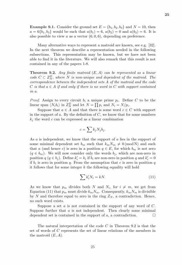
Example 9.1. Consider the ground set E = {b1, b2, b3} and N = 10, thena = 6{b1, b3} would be such that a(b1) = 6, a(b2) = 0 and a(b3) = 6. It isalso possible to view a as a vector (6, 0, 6), depending on preference.

Many alternative ways to represent a matroid are known, see e.g. [32].In the next theorem we describe a representation needed in the followingsubsections. This representation may be known, but we have not beenable to find it in the literature. We will also remark that this result is notcontained in any of the papers 1-8.

Theorem 9.2. Any finite matroid (E,A) can be represented as a linearcode C ⊂ ZE

N , where N is non-unique and dependent of the matroid. Thecorrespondence between the independent sets A of the matroid and the codeC is that a ∈ A if and only if there is no word in C with support containedin a.

Proof. Assign to every circuit bi a unique prime pi. Define C to be thelinear span ⟨Nibi⟩ in ZE

N and let N =∏

pi and Ni = N/pi.

Suppose that a ∈ A and that there is some word c ∈ C with supportin the support of a. By the definition of C, we know that for some numberskj the word c can be expressed as a linear combination

c =∑

kjNjbj .

As a is independent, we know that the support of a lies in the support ofsome minimal dependent set bm such that kmNm ∕= 0 (modN) and suchthat a (and hence c) is zero in a position q ∈ E, for which bm is not zero(q ∈ bm). We will now consider only the words bj , which are non-zero inposition q (q ∈ bj). Define k′i = ki if bi are non-zero in position q and k′i = 0if bi is zero in position q. From the assumption that c is zero in position qit follows that for some integer k the following equality will hold

∑k′iNi = kN. (11)

As we know that pm divides both N and Ni, for i ∕= m, we get fromEquation (11) that pm must divide kmNm. Consequently, kmNm is divisibleby N and therefore equal to zero in the ring ZN , a contradiction. Hence,no such word exists.

Suppose a set a is not contained in the support of any word of C.Suppose further that a is not independent. Then clearly some minimaldependent set is contained in the support of a, a contradiction.

The natural interpretation of the code C in Theorem 9.2 is that theset of words of C represents the set of linear relations of the members inthe matroid (E,A).

25

26

10 The error correcting property

There are many ways in which an e-error correcting code can be repre-sented. The most naive representation is to simply make a dictionary of allwords and in the dictionary translate each of the words into a code word.It is easy to see that this is always possible if we have pairwise disjointspheres of radius e around all code words.

We will only consider constructions where we define a code by consid-ering a set of code words C such that the code words is mapped into someset B under multiplication with some matrix A. We will in this section seethat this construction is in fact possible for any code. We can also regardA as a row-vector with elements from the ground set E of some matroid.In the context when the columns of A are considered to be elements ofsome general matroid we will below consider the code representation C ′ ofthis matroid for some N as given by Theorem 9.2. We define equality usingthis code C ′.

Example 10.1. Consider some elements b1, b2, b3 in some matroid. Then

4b1 + 3b2 = 7b3,

if (4, 3,−7, 0, 0, . . . ) ∈ C ′.

Observe that, if the elements of the matroid are not possible to repre-sent as vectors (and hence A as a matrix), then the representation of thecode will always be in a ring which is not a field.

We will start with some well known and very nice properties of linearcodes.

Theorem 10.2. A linear code is an e-error correcting code, for a positiveinteger e, if and only if the minimum (non-zero) weight of a code word isat least 2e+ 1.

Proof. If the code is e-error correcting then the statement is trivial as thezero word belongs to the code.

Suppose the minimum weight code word condition is true and that thecode is not e-error correcting. We then know that there exist two wordsc and c′ at distance 2e or less. The code is linear and hence c − c′ ∈ C.However, by assumption the only word of weight less than 2e+1 is the zeroword, hence c = c′.

The first and most basic definition of a code using matrix multiplica-tion is that C = {c∣Ac = 0}. Observe that this imply that C is a linearcode. This construction was used in 1940’s by Hamming to give the firstconstruction of perfect codes, the Hamming codes [9]. The following theo-rem is also well known.

Theorem 10.3. A code C = {c∣Ac = 0} is an e-error correcting code ifand only if every set of 2e-columns of A is independent.

26

27

b1 b2 b3

b4b5

b6

b7

Figure 9: The Fano matroid.

Proof. Suppose that every set of 2e-columns is independent. Then anydependent set must be of size 2e + 1 or larger, and hence the minimumweight word (the smallest dependent set) is of size at least 2e+ 1.

Suppose that the code C is e-error correcting. Then the minimumdistance is at least 2e+1 and hence the smallest dependent set must be ofsize 2e+ 1 or larger.

Corollary 10.4. Every binary matrix A with non-zero and different columnsdefines a linear 1-error correcting code.

Corollary 10.5. (Hamming codes)Every binary matrix A of size n × (2n − 1) with non-zero and differentcolumns defines a perfect linear 1-error correcting code.

Another example of a binary linear perfect code is the Golay code oflength 23, which is a linear binary perfect 3-error correcting code, discov-ered in 1948 by Golay [8].

During the first part of the history of perfect codes one believed thatonly linear perfect codes existed. This was for example conjectured byShapiro and Slotnik in 1956 [28]. This conjecture was later disproved byan example given by Vasil’ev in 1962 [31].

Any binary matrix defining a linear code as described above is calleda parity check matrix for the corresponding code.

Observe that Theorem 10.3 implies that we could try to define er-ror correcting codes from any matroid, not only from those that we canrepresent as a subset of a vector space.

27

28

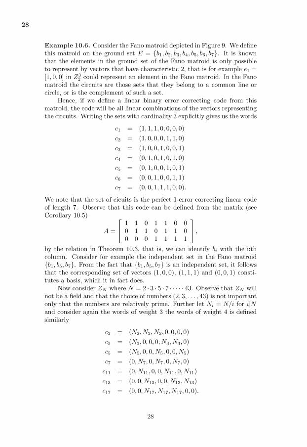
Example 10.6. Consider the Fano matroid depicted in Figure 9. We definethis matroid on the ground set E = {b1, b2, b3, b4, b5, b6, b7}. It is knownthat the elements in the ground set of the Fano matroid is only possibleto represent by vectors that have characteristic 2, that is for example e1 =[1, 0, 0] in Z3

2 could represent an element in the Fano matroid. In the Fanomatroid the circuits are those sets that they belong to a common line orcircle, or is the complement of such a set.

Hence, if we define a linear binary error correcting code from thismatroid, the code will be all linear combinations of the vectors representingthe circuits. Writing the sets with cardinality 3 explicitly gives us the words

c1 = (1, 1, 1, 0, 0, 0, 0)

c2 = (1, 0, 0, 0, 1, 1, 0)

c3 = (1, 0, 0, 1, 0, 0, 1)

c4 = (0, 1, 0, 1, 0, 1, 0)

c5 = (0, 1, 0, 0, 1, 0, 1)

c6 = (0, 0, 1, 0, 0, 1, 1)

c7 = (0, 0, 1, 1, 1, 0, 0).

We note that the set of cicuits is the perfect 1-error correcting linear codeof length 7. Observe that this code can be defined from the matrix (seeCorollary 10.5)

A =

⎡⎣

1 1 0 1 1 0 00 1 1 0 1 1 00 0 0 1 1 1 1

⎤⎦ ,

by the relation in Theorem 10.3, that is, we can identify bi with the i:thcolumn. Consider for example the independent set in the Fano matroid{b1, b5, b7}. From the fact that {b1, b5, b7} is an independent set, it followsthat the corresponding set of vectors (1, 0, 0), (1, 1, 1) and (0, 0, 1) consti-tutes a basis, which it in fact does.

Now consider ZN where N = 2 ⋅ 3 ⋅ 5 ⋅ 7 ⋅ ⋅ ⋅ ⋅ ⋅ 43. Observe that ZN willnot be a field and that the choice of numbers (2, 3, . . . , 43) is not importantonly that the numbers are relatively prime. Further let Ni = N/i for i∣Nand consider again the words of weight 3 the words of weight 4 is definedsimilarly

c2 = (N2, N2, N2, 0, 0, 0, 0)

c3 = (N3, 0, 0, 0, N3, N3, 0)

c5 = (N5, 0, 0, N5, 0, 0, N5)

c7 = (0, N7, 0, N7, 0, N7, 0)

c11 = (0, N11, 0, 0, N11, 0, N11)

c13 = (0, 0, N13, 0, 0, N13, N13)

c17 = (0, 0, N17, N17, N17, 0, 0).

28

29

Observe that this is the code C as defined in the proof of Theorem 9.2. Itfollows that this code represents the Fano matroid and that C is 1-errorcorrecting.

The example above illustrates a general result about the code repre-sentation of a matroid.

Corollary 10.7. Any code C as defined in Theorem 9.2 is a linear e-errorcorrecting code, where e is the largest integer such that 2e+1 is smaller orequal to the cardinality of the minimal cardinality of a dependent set.

Above we defined a linear code by the relation C = {c ∣Ac = 0}. Anatural generalization is to consider a set B such that the zero word belongsto B and define the code as C = {c ∣Ac ∈ B}. This definition leads to thefollowing result that must be well known.

Theorem 10.8. Let A be a row vector with elements from some matroid(E,F ). Let N be an integer such that the matroid (E,F ) is possible torepresent as a code with members in ZE

N (see Theorem 9.2). Further, letB ⊂ E be a set such that 0 ∈ B and such that for every member b of B,there exists c ∈ Zn

N such that Ac = b.For any code C = {c ∈ Zn

N ∣Ac = xbi , bi ∈ B , x ∈ ZN}, the statementthat C is an e-error correcting code is equivalent to the statement that forany set D ⊂ A such that ∣D∣ = 2e and any set G ⊂ B, such that ∣G∣ ≤ 2and 0 ∕∈ G then D ∪G is independent.

Proof. Observe that there are three distinct possible cases for the set G

i) G = {b1, b2} for two different non-zero elements b1 and b2 in B,ii) G = {b1} for a non-zero elements b1 in B,iii) G = ∅.

Suppose that the code C is e-error correcting. Consider two differentand non-zero words b1, b2, such that they minimize the cardinality of theset D, where D is the minimal set such that the set D ∪ {b1} ∪ {b2} isdependent. Observe that the cases with only one b1 or no such elementwill give a larger set D. Further, we know that the weight of the non-zeroword of minimum weight is at least 2e + 1. This proves the cases ii) andiii). Moreover in case i) this imply that if D has smaller cardinality than2e + 1, then the corresponding choice of coefficients is such that both b1and b2 have non-zero coefficients x1 and x2 (otherwise there is a code wordwith support D). Take any word c1 such that Ac1 = b1. Consider the twocode words x1c1 and c2 = x1c1 + d and observe that they differ only in thepositions given by D. Hence it follows that ∣D∣ > 2e.

Take two different words c1 and c2 such that they give the minimumdistance of the code C. Let d = c1 − c2, that is, w(d) is the minimumdistance of C. From the definition of the code C we know that Ac1 = x1b1

29

30

and Ac2 = x2b2 for some members b1, b2 ∈ B. It follows that Ad− x1b1 +x2b2 = 0. Let D be the support of d. Consider now the three possiblecases. In the first case when b1 and b2 are different and non-zero, we shallconsider the set D∪{b1}∪{b2}. In the second case one (i.e. b1) is non-zeroand the other word b2 is equal to b1 or zero. In that case we shall considerthe set D ∪ {b1}. In the third and final case when both b1 and b2 are zero,we shall consider the set D. The observation we make is that the set weare considering is dependent. From this we may conclude that the weightof d must be at least 2e+ 1.

Observe that this theorem also implies that we could consider othermatroids than those possible to represent as a set in a vector space, but itseems to have little practical use to do so.

Theorem 10.9. Every code C such that 0 ∈ C can be represented asC = {c∣Ac = xbi , bi ∈ B}.Proof. Let A = Id, B = C and all coefficients belong to the binary field,these conditions imply that C = {c∣ c ∈ C}.

Note that for the choice of representation in the proof of Theorem 10.9,Theorem 10.8 becomes ”a code is e-error correcting if and only if all wordsdiffer in at least 2e+ 1 positions”.

A concept that is closely related to binary error correcting codes isthat of binary tilings. We will in the next subsection give the definitionand some general results for tilings.

11 Binary tilings

Two subsets A and B of the binary vector space Zn2 is a tiling (A,B) if for

every d ∈ Zn2 there is a unique pair ai ∈ A , bj ∈ B such that d = ai + bj .

Observe that as a consequence we know that ∣A∣ = 2m and ∣B∣ = 2n−m, forsome integer m. Binary tilings are closely related to perfect codes, considerfor example the following explicit example.

Example 11.1. Consider the tiling (C,E) for the linear perfect code oflength 3

(C,E) =

⎛⎝

0 10 1 ,0 1

0 1 0 00 0 1 00 0 0 1

⎞⎠ .

In the later sections about codes we will need the following result aboutbinary tilings.

30

31

Lemma 11.2. The following statements are equivalenti) The pair (¾(A), ¾(B)) is a tiling for some automorphism ¾ of Zn

2 .ii) The pair (¾(A), ¾(B)) is a tiling for any automorphism ¾ of Zn

2 .iii) The pair (A + a,B + b) is a tiling for some pair of words a ∈ Zn

2 andb ∈ Zn

2 .iv) The pair (A + a,B + b) is a tiling for any pair of words a ∈ Zn

2 andb ∈ Zn

2 .

Proof. By renaming the sets we can assume that (A,B) is a tiling. Thenumber of elements in the two sets is such that it is sufficient to prove thatfor any ¾ ∈ Aut(Zn

2 ) and any d ∈ Zn2 their exists some ¾(ai) + ¾(bj) =

d. The tiling condition gives that their exists ai ∈ A, bj ∈ B such that¾−1(d) = ai + bj . Hence d = ¾(ai) + ¾(bj). This proves i) and ii).

Again with similar arguments, suppose (A,B) is a tiling and d ∈ Zn2 .

By assumption there exist aj , bj such that d + a + b = aj + bj and henced = (aj + a) + (bj + b), where clearly aj + a ∈ A + a and bj + b ∈ B + b.This proves iii) and iv).

In all following sections we will assume that all tilings (A,B) are suchthat A ∩B = 0.

Theorem 11.3. For every binary tiling (A,B) such that ∣A∣ = 2m, ∣B∣ =2n−m and any index j for the words in A and B, the number of words inA with 1 in position j is 2m−1 or/and the number of words in B with 1 inposition j is 2n−m−1.

Proof. Suppose the number of words of A with 1 in position j is a and thatthe number of words of B with 1 in position j is b. The tiling conditionimplies that we need to get a one in exactly half of the combinations ofcolumns from A and B, that is, the following equation must be fulfilled

a2n−m + b2m − 2ab = 2n−1. (12)

By symmetry we can assume that b ∕= 2n−m−1. We then get that theequation (12) is equivalent to

a =2n−1 − b2m

(2n−m − 2b)= 2m−1.

We would like to remark that the weight condition described in Theo-rem 11.3 plus some additional conditions also will give sufficient conditionsfor two sets A and B to constitute a tiling (A,B). The proof of that factby Heden [10] uses the concept of Fourier coefficients and no direct proofof this fact is known so far.

31

32

12 Simplex codes

A simplex code is here defined to be a linear binary code of length n orn+1, where n = 2m−1 for some integer m, such that every non-zero wordhave weight (n+1)/2. By adding a zero position in the words of length n,it will in most contexts be sufficient to consider the case of length n+ 1.

Lemma 12.1. Let A be a k× (n+1) full-rank matrix, where n+1 = 2m.Then the row space of A is a simplex code if and only if A has as columnsevery member of Zk

2 repeated exactly 2m−k times.

Observe that this lemma, in the case of length n, differs in that thezero column would appear one time less than the other words in Zk

2 .

Proof. Consider any Zk2 and repeat every word in this space an equal num-

ber of times as columns in A. Clearly the row space will constitute asimplex code.

Proof by induction over the dimension k of the simplex code. It is clearthat any simplex code of dimension 1 have the property. Suppose that wehave k rows that define a simplex code. The k − 1 first of these rows willdefine a simplex code of dimension k − 1. We observe that the supportof the last row must intersect all non-zero words in the k − 1 dimensionalsimplex code in half of their supports. In particular this is true for the k−1first rows that we picked when defining the k−1 dimensional simplex code.By the induction hypothesis the first k− 1 positions contain every word inZk−12 at least twice. It follows that we will get all words in the space Zk

2

an equal number of times as the remaining row will split every set of wordsof Zk−1

2 into two sets, one by adding zero and one by adding a one in thek:th position of the column.

13 Binary perfect 1-error correcting codes

In this section we will only consider binary 1-error correcting perfect codesof length n = 2m − 1. We shall call such codes perfect codes for short.Recall that all perfect codes are sets C such that the words of C definesa disjoint covering of Zn

2 with radius 1-spheres. In the tiling notationthis is the same as saying that the pair (C,E) is a tiling for the set E ={0, e1, . . . , en}, where ei is the weight one word with support in position i,compare Example 11.1.

The rank of a perfect code is defined as the dimension of the linearspan ⟨C⟩ of the code.

A period of a code C is a word p ∈ Zn2 such that p+ C = C. The set

of all periods of the code C is called the kernel of C, ker(C). As we assumethat 0 ∈ C it follows that any period belongs to C, that is, ker(C) ⊂ C.

A natural problem to consider is for which parameters (n, r, k) doesthere exist a perfect code C, where n is the length, r the rank and k

32

33

the dimension of the kernel of the perfect code C. This so called ”EtzionVardy”-problem posed in 1998 [5] was solved in a number of steps, see forexample [3, 12, 23, 26, 30]. We will not give the details here, only note thatthis problem was not laid to rest until very recently (2006). The final stepwas completed by Heden [11].

The definition of the kernel gives a natural disjoint covering of a perfectcode. For m = ∣C∣/∣ ker(C)∣ − 1 there are words ci such that

C = ker(C) ∪ (c1 + ker(C)) ∪ ⋅ ⋅ ⋅ ∪ (cm + ker(C)).

One of the first non-trivial properties discovered about perfect codes is thatall perfect codes have a unique number of words with a specific weight [28].

Theorem 13.1. The function fni (C) = ∣{c∣w(c) = i , c ∈ C}∣ where C is

a perfect code of length n is independent of the perfect code C.

Proof. Proof by induction. We know by assumption that fn0 = 1. Assume

that fni is uniquely determined for i < j. Consider the words of weight

j − 1. Every such word is either a code word or a neighbour to a codeword. This fact gives the equation

(n

j − 1

)= (n− j + 2) ⋅ fn

j−2 + j ⋅ fnj + fn

j−1,

which determine the value of fnj and hence proves the statement.

Observe that the equality is derived using only the fact that the radius1-balls around code words are disjoint and cover Zn

2 . This property ispreserved if we translate a perfect code C to the translated perfect coded + C for any word d. This follows as the mapping +d is an isometricmapping, that is, it preserve the distance between any two words c1 andc2,

±(c1, c2) = ±(c1 + d, c2 + d) = w((c1 + d)− (c2 + d)) = w(c1 − c2).

Theorem 13.2. fni = fn

n−i.

Proof. Consider first the all one word. Either it is contained in the code orthere will be just one single word of weight n − 1. Consider secondly therecursion used in the proof of Theorem 13.1. We observe that the formulagiving the recursion will also work if we start the recursion with the numberof words with weight n. This implies that if the all one word belongs tothe set of code words, then the theorem follows by symmetry. Supposethat the all one word does not belong to the code. In that case we havea unique word c of weight n − 1 in the code. We then know that startingthe recursion with 0 words of weight n always will give that there mustbe one word of weight zero. Pick some i in the support of c and considerthe translated perfect code C + ei (where ei is the weight one word withsupport in i). As the minimum distance is three this code does not containthe all one word either. Hence, by the recursion it contains the zero word,which is a contradiction as this would imply that ei ∈ C.

33

34

Note that, as a consequence of the above theorem, we know that theall one word will always belong to every perfect code C. In fact somethingeven stronger is true and well known [28].

Theorem 13.3. The all one word 1 is contained in the kernel of everyperfect code C.

Proof. We need to prove that for every c ∈ C then c+1 ∈ C. Consider theperfect code c+ C then 1 ∈ c+ C and hence c+ 1 ∈ C.

Closely related to perfect codes is the concept of extended perfectcodes. Extended perfect codes are often needed when working with andconstructing perfect codes, as we will see in later sections.

13.1 Extended perfect codes

Consider the injective linear function f+ from Zn2 to Zn+1

2

f+(c1, . . . , cn) = (c1, . . . , cn,∑

ci).

For every perfect code C we can get a new 1-error correcting codeC+ = {f+(c)∣c ∈ C}. Codes of the type C+ are denoted by extendedperfect codes. It is easy to see that an extended perfect code have minimumdistance 4. Further we can also consider the surjective function f− fromZn+12 to Zn

2

f−(c1, . . . , cn, cn+1) = (c1, . . . , cn).

Obviously f− ∘ f+ = Id.

13.2 Equivalence and mappings of perfect codes I

If we consider an error correcting code as some set that fulfils a minimumdistance criteria, then it is very natural to consider two perfect codes C andC ′ of length n as equivalent if there exists some isometric mapping of Zn

2

that maps C on C ′. We get a different equivalence relation if we considertwo codes as equivalent if there is a linear bijective mapping on Zn

2 , thatmaps C on C ′. In all further discussions we will mean isometric equivalencewhen we refer two codes as equivalent and if we state that two codes arelinearly equivalent we will mean that there is a linear bijective mappingon Zn

2 that maps C on C ′. In some cases we will also talk about linearlyequivalent sets (codes). If these sets do not have a common representation,then the linear bijective map is between the linear span of the sets, that is⟨C⟩ and ⟨C ′⟩.

A well know and very useful property is given in the following wellknown theorem which also gives a canonical representation of an isometricmapping between binary spaces.

34

35

Theorem 13.4. Every isometric mapping !: Zn2 → Zn

2 , can be written as!(c) = ¼(c) + c0 for a unique word c0 and a unique permutation ¼.

Proof. Clearly we must pick c0 = !(0). Further we know from the isometricproperty that !(ei) = c0 + ej , for some index j. Remember that ei is theweight one word with support in i. Hence it is clear that we can definea unique permutation ¼ from this action, that is, we define ¼(i) = j. Itremains to prove that for this choice of ¼, !(c) = ¼(c) + c0 for arbitrary c.Proof by induction over the weight of code words. Suppose the equality istrue for all words of weight p such that p < q. For every i in the supportof c let ci be the word with weight q − 1 such that ci + ei = c, then bythe induction hypothesis !(ci) = ¼(ci) + c0. By the isometric property itfollows that !(c) = ¼(ci) + c0 + ej for some index j. Further we know that!(ei) = c0 + ¼(ei), hence q − 1 = ±(!(c), !(ei)) = ±(¼(ci) + ej , ¼(ei)). Itremains to prove that ej = ¼(ei). We know that ej is either equal to ¼(ei)or in the support of ¼(ci). Suppose that they are not equal. Then this factimplies that !(ci + ¼−1(ej)) = ¼(ci) + ej + c0. Furthermore, the fact that! is injective implies that ci+¼−1(ej) = c, which is a contradiction. Hencewe can conclude that ej = ¼(ei).

Define the symmetry group Sym(C) of a perfect code C to be thegroup of permutations ¼ such that ¼(C) = C. We define here the auto-morphism group Aut(C) to be the group of bijective linear mappings ¾such that ¾(C) = C and finally let the isometry group Iso(C) be all theisometric mappings ! such that !(C) = C. Observe that it is commonin coding theory to use the convention to denote the isometric group bythe automorphism group. This can cause confusion when reading articlesabout coding theory and we believe that our terminology would be better.Further it is clear that

Sym(C) ⊂ Aut(C)

andSym(C) ⊂ Iso(C).

The following theorem is well known, but we again include a proof forcompleteness.

Theorem 13.5. The symmetry group of a linear perfect code C of lengthn is isomorphic to the general linear group GL(n, log2(n+ 1)).

Proof. Let A be the parity check matrix of C, that is C = {c∣Ac = 0}.Suppose ¼ ∈ Sym(C). Then ¼(A) will be a parity check matrix for thecode C. However the dual space is fixed, and hence ¼ only changes thebasis for the row space of A. We can conclude that ¼(A) = BA forB ∈ GL(n, log2(n+ 1)).

Suppose that B ∈ GL(n, log2(n+1)). We know that A contains every

non-zero vector of Zlog(n+1)2 . Consequently B is a permutation ¼ of the

columns of A.

35

36

Before we continue this discussion of the automorphism group of acode C we need a systematic way to structure the linear properties of aperfect code.

13.3 The coset structure of a perfect code

In Paper 5 a systematic way of factoring the linear structure of a perfectcode was presented. The terminology used in that paper was a bit unfor-tunate as it was a direct translation of the Swedish terminology. Here wewill therefore use the terminology ”the coset structure” instead of ”the sideclass structure”. We hope this will avoid some of the misunderstandingsthat seem to have been caused by the old terminology.

To every perfect code we will associate a basis ci, i ∈ [1, r] to the space⟨C⟩ such that, for i = 1 . . . k, ci ∈ ker(C), where k is the dimension of thekernel and r is the rank of the code. We extend this basis to a basis ofZn2 by using some words cr+1 . . . cn. Note that ci, for k < i ≤ r, do not

necessarily lie in the code C. Consider the matrix

A = [ck+1, . . . , cr].

This matrix defines the (non-unique) coset structure of the code C as theset SC defined by

SC = {s ∈ Zr−k2 ∣As ∈ C}.

Observe that SC depends upon which basis we choose and in which orderwe place this basis in A, but it is clear that 0 ∈ SC . We will see by theresults in this section that the ”non-uniqueness” is not a problem as wecan think of SC as an equivalence class under the set of bijective linearmappings. We also need to consider the full rank matrix

Ae = [c1, . . . , cn]. (13)

Observe that it follows from the definition of the coset structure that theset SC must be aperiodic, that is for any non-zero s ∈ SC we know thats + SC ∕= SC , otherwise As would belong to the kernel of C. We willsometimes omit the index C when it is clear which code we are workingwith.

The definition of the coset structure gives us a very practical decom-position of a code in the following way

C = AeSe, (14)

where the set Se = Zk2 × S × 0n−r.

The following theorem first appeared in Paper 5.

Theorem 13.6. Two perfect codes C and C ′ of the same length n, arelinearly equivalent if and only if there exists a linear bijective mapping !on Zr−k

2 such that SC′ = !(SC).

36

37

Proof. Suppose that ¾ exists. Represent this mapping with a matrix B.Then by assumption we know that BC = C ′, which is equivalent toBAeSe = Ae

′S′e. Hence (Ae

′)−1BAeSe = S′e. Let D = (Ae

′)−1BAe.For any word c ∈ ker(C) we know by linearity and the definition of S thatBc ∈ ker(C ′). It follows that D will map {ei} for i ∈ [1, k] to a basis forZk2 ×0n−k. Next pick any basis B ⊂ S for S and consider 0k×B×0n−r. Let

P : Zn2 → Zr−k

2 , be the projection on the coordinate positions representingthe coset structure. By the bijectivity and the above fact that the kernelis mapped to the kernel we know that

P(D(0k ×B × 0n−r)

)

is a basis. Further, for every s ∈ S we have s =∑

¸ibi, for bi ∈ B, andthen D[0k, s, 0n−r]T ∈ C ′ if and only if [0k, s, 0n−r]T ∈ C. Hence D definesa linear bijective mapping !: S → S′ by defining it to be

!(bi) = P ∘D(bi),

and extending this linearly to all elements in S.

Suppose that ! exists. Then trivially we can extend this mapping to alinear bijective mapping B such that B(Zk

2 × S × 0n−r) = Zk2 × S′ × 0n−r.

It follows that we can define ¾ by the matrix Ae′BAe

−1.

The interpretation of the above theorem is that two codes are linearlyequivalent if their coset structures considered as matroids are the same. Infact something stronger is true as the following theorem reveals.

Theorem 13.7. Two sets of binary vectors S and S′ are linearly equivalentif and only if they represent the same matroid.

Proof. Clearly two linearly equivalent sets of binary vectors represent thesame matroid.

Suppose two binary sets are the same when considered as two matroids(S,A) and (S′, A′). Then by definition there is a bijective function ¾ suchthat ¾(a) for a ∈ 2S independent, i.e. ¾(a) ∈ A′, if and only if a ∈ A.Pick any set ab of maximal cardinality in A. Then ¾(ab) ∈ A′ and ¾(ab)will also be of maximal cardinality in A′. Clearly, by the bijectivity of ¾,∣ab∣ = ∣¾(ab)∣. Further, the maximal cardinality implies that ab is a basisfor ⟨S⟩ and that ¾(ab) is a basis for ⟨S′⟩. We can therefore pick a linearbijective mapping D from ⟨S⟩ to ⟨S′⟩, such that for any ® ∈ ab,

D® = ¾(®).

Note that we extendD to sets in the same way as ¾, that isD{®i} = {D®i}.Observe that for any independent set a of binary vectors, a∪s is a minimaldependent set if and only if (

∑®∈a ®) + s = 0. Moreover s is a unique

37

38

element. Pick any s ∈ S. Then there is a unique set a ⊂ ab, such that a∪ sis minimal dependent set. It follows that

Ds = D(∑®∈a

®) =∑®∈a

D® = ¾(s).

As we have previously remarked, it is sometimes more convenient towork with extended perfect codes. If we for example consider isometricequivalence, extending the code can change the correspondence betweentwo codes. For example if we extend a code C in the last coordinateposition and then remove some other coordinate position, we may get acode C ′, which is not isometric equivalent to C. The precise conditionsunder which they are isometric equivalent were solved by V. A. Zinovievand D. V. Zinoviev [33]. The following theorem shows that this situationdoes not occur when linear equivalence is considered.

Theorem 13.8. Two extended perfect codes C+ and (C ′)+ are linearlyequivalent if and only if the corresponding perfect codes C and C ′ are lin-early equivalent.

Proof. We can without loss of generality assume that we always add andremove position n+ 1.

If (C+)′ = Á(C+) then C ′ = f−(Á(f+(C)) will be a bijective mapping,and hence C is linearly equivalent with C ′.

Suppose C ′ = Á(C). Observe that we cannot use the mapping f+ ∘Á∘f− as this map is only a bijection on the set of even weight words. Supposewe represent Á as a matrix

A =

⎛⎜⎜⎜⎜⎝

− a1 −− ⋅ −− ai −− ⋅ −− an −

⎞⎟⎟⎟⎟⎠

.

Let Á+ be the following linear map

T =

(A 0a 1

). (15)

where a is the sum of the rows in A plus the all one word,∑

ai+1. Observethat A has full rank and hence that T has full rank. In order to check thatthis is a correct mapping we simply need to check that every word in C+ ismapped to a word in (C ′)+. Consider any word c in the code C+. Clearlyc have even weight and hence 1 ⋅ c = 0 and Tc = [Ac−,

∑ai ⋅ c−]T . We

know from the assumptions that Ac− = (c′)− which belongs to C ′. Hence,adding a parity to this word gives us a word in (C ′)+.

38

39

Theorem 13.9. A non-singular linear map of Zn2 represented by a matrix

A−1 maps a perfect code C onto a perfect code C ′ if and only if (C,D) is atiling, where D is the set containing the columns of the matrix A plus theall zero column.

Proof. Suppose C ′ = A−1C. Then we know that (A−1C,E) is a tiling,where E = {0, e1 . . . en}. Hence (C,DE) is a tiling by Lemma 11.2.

Suppose (C,D) tiling. Then (A−1C,E) is a tiling which implies thatC ′ = A−1C is a perfect code.

One may call any set with the same properties as the set D in Theo-rem 13.9 an error set. This terminology comes from the observation thatthese sets are all possible full rank sets such that we, for the perfect code C,get a tiling (C,D). One example of an error sets is the set E = {0, e1 . . . en}containing the weight one errors. A natural question to ask is if it is possi-ble to find a set D, that does not have full rank and is such that 0 ∈ D andsuch that (C,D) is a tiling for some perfect code C. It is easy to see thatthere are always such sets as we can to each non-zero odd element in anerror set add the all one-word (or any other odd weight word in the kernel).This will turn the error set into a set containing only words of even weight.The easiest example is

A =

⎛⎝

010101

∣∣∣∣∣∣

001101010110

⎞⎠ .

In fact the following theorem will be true.

Theorem 13.10. For any perfect code C every full-rank set D = {ei +ci∣ci ∈ ker(C) , i ∈ [1, n]} ∪ {0} gives a mapping D−1 which maps C ontoa perfect code C ′ = D−1C.

Proof. By definition C and C + ei, i = 1, 2, . . . , n, give a disjoint coveringof Zn

2 . Hence the theorem follows from the fact that C + ei + ci = C + eiand Theorem 13.9.

Further we can also derive the following lemma.

Lemma 13.11. For any perfect code C and every full-rank matrix D−1

such that C ′ = D−1C is a perfect code, the error set D is on the formD = {ei + ci∣ci ∈ C} ∪ {0}.Proof. By the definition of a perfect code any word not in C can be writtenas ci+ei. Hence every mapping can be written on the form stipulated.

Theorem 13.12. Let C = AeZk2 ×S×0n−r be any perfect code with coset

structure S. Then a non-singular linear map ¾ is an automorphism of Cif and only if there exists a map ° ∈ Aut(S) such that

¾ (Ae(z1, s, 0)) = Ae(z2, °(s), 0),

for any words z1 and z2 in Zk2 .

39

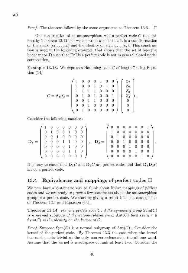
40

Proof. The theorem follows by the same arguments as Theorem 13.6.

One construction of an automorphism ¾ of a perfect code C that fol-lows by Theorem 13.12 is if we construct ¾ such that it is a transformationon the space ⟨c1, . . . , ck⟩ and the identity on ⟨ck+1, . . . , cr⟩. This construc-tion is used in the following example, that shows that the set of bijectivelinear maps D such that DC is a perfect code is not in general closed undercomposition.

Example 13.13. We express a Hamming code C of length 7 using Equa-tion (14)

C = AeSe =

⎛⎜⎜⎜⎜⎜⎜⎜⎜⎝

1 0 0 0 1 0 01 0 0 1 0 1 01 1 1 1 0 0 00 1 0 1 0 0 10 0 1 1 0 0 00 0 1 0 0 0 00 1 0 0 0 0 0

⎞⎟⎟⎟⎟⎟⎟⎟⎟⎠

⎧⎨⎩

Z2

Z2

Z2

Z2

000

⎫⎬⎭

.

Consider the following matrices

D1 =

⎛⎜⎜⎜⎜⎜⎜⎜⎜⎝

1 0 0 0 0 0 00 1 0 0 1 0 00 0 1 0 0 0 00 0 0 1 1 0 00 0 0 0 1 0 00 0 0 0 1 1 00 0 0 0 0 0 1

⎞⎟⎟⎟⎟⎟⎟⎟⎟⎠

, D2 =

⎛⎜⎜⎜⎜⎜⎜⎜⎜⎝

0 0 0 0 0 0 11 0 0 0 0 0 00 1 0 0 0 0 00 0 1 0 0 0 00 0 0 1 0 0 00 0 0 0 1 0 00 0 0 0 0 1 0

⎞⎟⎟⎟⎟⎟⎟⎟⎟⎠

.

It is easy to check that D1C and D2C are perfect codes and that D1D2Cis not a perfect code.

13.4 Equivalences and mappings of perfect codes II

We now have a systematic way to think about linear mappings of perfectcodes and we are ready to prove a few statements about the automorphismgroup of a perfect code. We start by giving a result that is a consequenceof Theorem 13.1 and Equation (14).

Theorem 13.14. For any perfect code C, if the symmetry group Sym(C)is a normal subgroup of the automorphism group Aut(C) then every ¼ ∈Sym(C) is the identity on the kernel of C.

Proof. Suppose Sym(C) is a normal subgroup of Aut(C). Consider thekernel of the perfect code. By Theorem 13.3 the case when the kernelhas rank one is trivial as the only non-zero element is the all-one word.Assume that the kernel is a subspace of rank at least two. Consider the

40

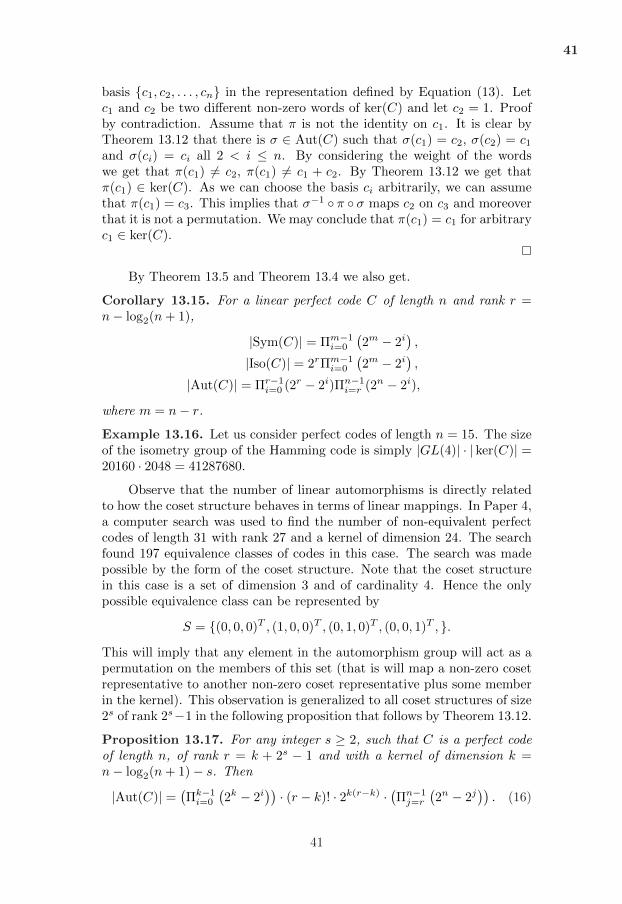
41

basis {c1, c2, . . . , cn} in the representation defined by Equation (13). Letc1 and c2 be two different non-zero words of ker(C) and let c2 = 1. Proofby contradiction. Assume that ¼ is not the identity on c1. It is clear byTheorem 13.12 that there is ¾ ∈ Aut(C) such that ¾(c1) = c2, ¾(c2) = c1and ¾(ci) = ci all 2 < i ≤ n. By considering the weight of the wordswe get that ¼(c1) ∕= c2, ¼(c1) ∕= c1 + c2. By Theorem 13.12 we get that¼(c1) ∈ ker(C). As we can choose the basis ci arbitrarily, we can assumethat ¼(c1) = c3. This implies that ¾−1 ∘ ¼ ∘ ¾ maps c2 on c3 and moreoverthat it is not a permutation. We may conclude that ¼(c1) = c1 for arbitraryc1 ∈ ker(C).

By Theorem 13.5 and Theorem 13.4 we also get.

Corollary 13.15. For a linear perfect code C of length n and rank r =n− log2(n+ 1),

∣Sym(C)∣ = Πm−1i=0

(2m − 2i

),

∣Iso(C)∣ = 2rΠm−1i=0

(2m − 2i

),

∣Aut(C)∣ = Πr−1i=0 (2

r − 2i)Πn−1i=r (2

n − 2i),

where m = n− r.

Example 13.16. Let us consider perfect codes of length n = 15. The sizeof the isometry group of the Hamming code is simply ∣GL(4)∣ ⋅ ∣ ker(C)∣ =20160 ⋅ 2048 = 41287680.

Observe that the number of linear automorphisms is directly relatedto how the coset structure behaves in terms of linear mappings. In Paper 4,a computer search was used to find the number of non-equivalent perfectcodes of length 31 with rank 27 and a kernel of dimension 24. The searchfound 197 equivalence classes of codes in this case. The search was madepossible by the form of the coset structure. Note that the coset structurein this case is a set of dimension 3 and of cardinality 4. Hence the onlypossible equivalence class can be represented by

S = {(0, 0, 0)T , (1, 0, 0)T , (0, 1, 0)T , (0, 0, 1)T , }.This will imply that any element in the automorphism group will act as apermutation on the members of this set (that is will map a non-zero cosetrepresentative to another non-zero coset representative plus some memberin the kernel). This observation is generalized to all coset structures of size2s of rank 2s−1 in the following proposition that follows by Theorem 13.12.

Proposition 13.17. For any integer s ≥ 2, such that C is a perfect codeof length n, of rank r = k + 2s − 1 and with a kernel of dimension k =n− log2(n+ 1)− s. Then

∣Aut(C)∣ = (Πk−1

i=0

(2k − 2i

)) ⋅ (r − k)! ⋅ 2k(r−k) ⋅ (Πn−1j=r

(2n − 2j

)). (16)

41

42

Note that for any choice of parameters such that n = 2m − 1 and suchthat r ≤ n in Proposition 13.17, there exists a perfect code. This will followby a construction similar to that in a later subsection, see Example 13.26.

Theorem 13.18. If two extended perfect codes C and C ′ are linearly equiv-alent then there is a linear bijective map Á such that C ′ = Á(C) whichpreserves the parity of every vector in V n+1.

Proof. By the proof of Theorem 13.8 we can for every bijective linear mapÁ′, such that C ′ = Á′(C) construct a new linear map Á defined by thematrix

T =

(A 0a 1

), (17)

as defined in (15). We observe that the two mappings are identical whenrestricted to the code C. Trivially by the bijectivity it is sufficient to provethat all even weight words are mapped to even weight words. Let c be anyword of even weight. Then this word is mapped to [Ac−,

∑ai ⋅c−]+1⋅c]T =

[Ac−,∑

ai ⋅ c−]T .

13.5 The tiling representation (A,B) of a perfect codeC

In this subsection we shall be concerned with perfect codes. We will fre-quently need to represent a set both as a set and as a matrix. We will usethe convention that for any set A the matrix A is the matrix we get byarranging the non-zero words from A as columns in a matrix. Further wewill always consider codes as equal if they only differ by a permutation ofthe coordinate positions. The main observation is given in the followingwell known theorem, see [4].

Theorem 13.19. If (A,B) is a tiling then C = {c∣Ac ∈ B} is a perfectcode. Further the dual space of the row-space of A is contained in the kernelof C.

Proof. Let ai denote column number i of the matrix A and similarly formatrix B. Pick any word d. Then Ad = f and uniquely f = ai + bj , forai ∈ A and bj ∈ B, which implies that either ai ∕= 0 and then the wordd+ ei is the unique word at a distance of one from d or if ai = 0 and thend is a word in the code. The second part of the theorem follows directlyfrom the definition of the code C in this theorem and the definition of thekernel of a perfect code.

Theorem 13.20. Let C be any perfect code and D any subspace of thekernel of C. If A is a matrix with a basis for D⊥ as rows and B ={Ac∣ c ∈ C} then (A,B) is a tiling.

42

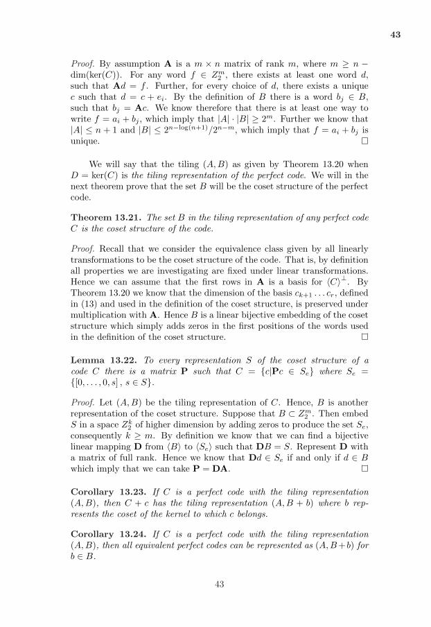
43

Proof. By assumption A is a m × n matrix of rank m, where m ≥ n −dim(ker(C)). For any word f ∈ Zm

2 , there exists at least one word d,such that Ad = f . Further, for every choice of d, there exists a uniquec such that d = c + ei. By the definition of B there is a word bj ∈ B,such that bj = Ac. We know therefore that there is at least one way towrite f = ai + bj , which imply that ∣A∣ ⋅ ∣B∣ ≥ 2m. Further we know that∣A∣ ≤ n + 1 and ∣B∣ ≤ 2n−log(n+1)/2n−m, which imply that f = ai + bj isunique.

We will say that the tiling (A,B) as given by Theorem 13.20 whenD = ker(C) is the tiling representation of the perfect code. We will in thenext theorem prove that the set B will be the coset structure of the perfectcode.

Theorem 13.21. The set B in the tiling representation of any perfect codeC is the coset structure of the code.

Proof. Recall that we consider the equivalence class given by all linearlytransformations to be the coset structure of the code. That is, by definitionall properties we are investigating are fixed under linear transformations.Hence we can assume that the first rows in A is a basis for ⟨C⟩⊥. ByTheorem 13.20 we know that the dimension of the basis ck+1 . . . cr, definedin (13) and used in the definition of the coset structure, is preserved undermultiplication with A. Hence B is a linear bijective embedding of the cosetstructure which simply adds zeros in the first positions of the words usedin the definition of the coset structure.

Lemma 13.22. To every representation S of the coset structure of acode C there is a matrix P such that C = {c∣Pc ∈ Se} where Se ={[0, . . . , 0, s] , s ∈ S}.

Proof. Let (A,B) be the tiling representation of C. Hence, B is anotherrepresentation of the coset structure. Suppose that B ⊂ Zm

2 . Then embedS in a space Zk

2 of higher dimension by adding zeros to produce the set Se,consequently k ≥ m. By definition we know that we can find a bijectivelinear mapping D from ⟨B⟩ to ⟨Se⟩ such that DB = S. Represent D witha matrix of full rank. Hence we know that Dd ∈ Se if and only if d ∈ Bwhich imply that we can take P = DA.

Corollary 13.23. If C is a perfect code with the tiling representation(A,B), then C + c has the tiling representation (A,B + b) where b rep-resents the coset of the kernel to which c belongs.

Corollary 13.24. If C is a perfect code with the tiling representation(A,B), then all equivalent perfect codes can be represented as (A,B+b) forb ∈ B.

43

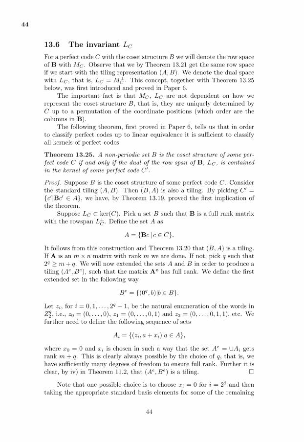
44

13.6 The invariant LC

For a perfect code C with the coset structure B we will denote the row spaceof B with MC . Observe that we by Theorem 13.21 get the same row spaceif we start with the tiling representation (A,B). We denote the dual spacewith LC , that is, LC = M⊥

C . This concept, together with Theorem 13.25below, was first introduced and proved in Paper 6.

The important fact is that MC , LC are not dependent on how werepresent the coset structure B, that is, they are uniquely determined byC up to a permutation of the coordinate positions (which order are thecolumns in B).

The following theorem, first proved in Paper 6, tells us that in orderto classify perfect codes up to linear equivalence it is sufficient to classifyall kernels of perfect codes.

Theorem 13.25. A non-periodic set B is the coset structure of some per-fect code C if and only if the dual of the row span of B, LC , is containedin the kernel of some perfect code C ′.

Proof. Suppose B is the coset structure of some perfect code C. Considerthe standard tiling (A,B). Then (B,A) is also a tiling. By picking C ′ ={c′∣Bc′ ∈ A}, we have, by Theorem 13.19, proved the first implication ofthe theorem.

Suppose LC ⊂ ker(C). Pick a set B such that B is a full rank matrixwith the rowspan L⊥

C . Define the set A as

A = {Bc ∣ c ∈ C}.It follows from this construction and Theorem 13.20 that (B,A) is a tiling.If A is an m× n matrix with rank m we are done. If not, pick q such that2q ≥ m+ q. We will now extended the sets A and B in order to produce atiling (Ae, Be), such that the matrix Ae has full rank. We define the firstextended set in the following way

Be = {(0q, b)∣b ∈ B}.Let zi, for i = 0, 1, . . . , 2q − 1, be the natural enumeration of the words inZq2 , i.e., z0 = (0, . . . , 0), z1 = (0, . . . , 0, 1) and z3 = (0, . . . , 0, 1, 1), etc. We

further need to define the following sequence of sets

Ai = {(zi, a+ xi)∣a ∈ A},where x0 = 0 and xi is chosen in such a way that the set Ae = ∪Ai getsrank m + q. This is clearly always possible by the choice of q, that is, wehave sufficiently many degrees of freedom to ensure full rank. Further it isclear, by iv) in Theorem 11.2, that (Ae, Be) is a tiling.

Note that one possible choice is to choose xi = 0 for i = 2j and thentaking the appropriate standard basis elements for some of the remaining

44

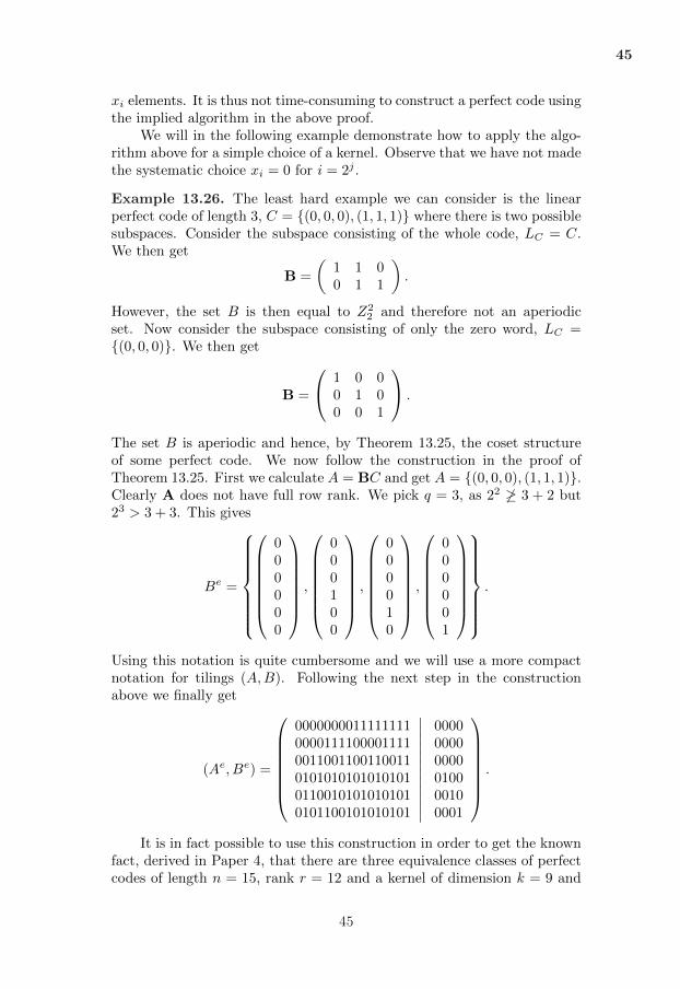
45

xi elements. It is thus not time-consuming to construct a perfect code usingthe implied algorithm in the above proof.

We will in the following example demonstrate how to apply the algo-rithm above for a simple choice of a kernel. Observe that we have not madethe systematic choice xi = 0 for i = 2j .

Example 13.26. The least hard example we can consider is the linearperfect code of length 3, C = {(0, 0, 0), (1, 1, 1)} where there is two possiblesubspaces. Consider the subspace consisting of the whole code, LC = C.We then get

B =

(1 1 00 1 1

).

However, the set B is then equal to Z22 and therefore not an aperiodic

set. Now consider the subspace consisting of only the zero word, LC ={(0, 0, 0)}. We then get

B =

⎛⎝

1 0 00 1 00 0 1

⎞⎠ .

The set B is aperiodic and hence, by Theorem 13.25, the coset structureof some perfect code. We now follow the construction in the proof ofTheorem 13.25. First we calculate A = BC and get A = {(0, 0, 0), (1, 1, 1)}.Clearly A does not have full row rank. We pick q = 3, as 22 ∕≥ 3 + 2 but23 > 3 + 3. This gives

Be =

⎧⎨⎩

⎛⎜⎜⎜⎜⎜⎜⎝

000000

⎞⎟⎟⎟⎟⎟⎟⎠

,

⎛⎜⎜⎜⎜⎜⎜⎝

000100

⎞⎟⎟⎟⎟⎟⎟⎠

,

⎛⎜⎜⎜⎜⎜⎜⎝

000010

⎞⎟⎟⎟⎟⎟⎟⎠

,

⎛⎜⎜⎜⎜⎜⎜⎝

000001

⎞⎟⎟⎟⎟⎟⎟⎠

⎫⎬⎭

.

Using this notation is quite cumbersome and we will use a more compactnotation for tilings (A,B). Following the next step in the constructionabove we finally get

(Ae, Be) =

⎛⎜⎜⎜⎜⎜⎜⎝

000000001111111100001111000011110011001100110011010101010101010101100101010101010101100101010101

∣∣∣∣∣∣∣∣∣∣∣∣

000000000000010000100001

⎞⎟⎟⎟⎟⎟⎟⎠

.

It is in fact possible to use this construction in order to get the knownfact, derived in Paper 4, that there are three equivalence classes of perfectcodes of length n = 15, rank r = 12 and a kernel of dimension k = 9 and

45

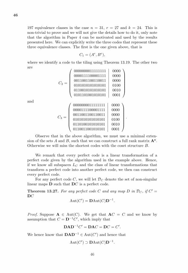
46

197 equivalence classes in the case n = 31, r = 27 and k = 24. This isnon-trivial to prove and we will not give the details how to do it, only notethat the algorithm in Paper 4 can be motivated and used by the resultspresented here. We can explicitly write the three codes that represent thesethree equivalence classes. The first is the one given above, that is

C1 = (Ae, Be),

where we identify a code to the tiling using Theorem 13.19. The other twoare

C2 =

⎛⎜⎜⎜⎜⎜⎜⎝

000000001111111100001111000011110011001100110011010101010101010101100101010101010101101001010101

∣∣∣∣∣∣∣∣∣∣∣∣

000000000000010000100001

⎞⎟⎟⎟⎟⎟⎟⎠

and

C3 =

⎛⎜⎜⎜⎜⎜⎜⎝

000000001111111100001111000011110011001100110011010101010101010101101001010101010110011001010101

∣∣∣∣∣∣∣∣∣∣∣∣

000000000000010000100001

⎞⎟⎟⎟⎟⎟⎟⎠

.

Observe that in the above algorithm, we must use a minimal exten-sion of the sets A and B, such that we can construct a full rank matrix Ae.Otherwise we will miss the shortest codes with the coset structure B.

We remark that every perfect code is a linear transformation of aperfect code given by the algorithm used in the example above. Hence,if we know all subspaces LC and the class of linear transformations thattransform a perfect code into another perfect code, we then can constructevery perfect code.

For any perfect code C, we will let DC denote the set of non-singularlinear maps D such that DC is a perfect code.

Theorem 13.27. For any perfect code C and any map D in DC , if C′ =

DCAut(C ′) = DAut(C)D−1.

Proof. Suppose A ∈ Aut(C). We get that AC = C and we know byassumption that C = D−1C ′, which imply that

DAD−1C ′ = DAC = DC = C ′.

We hence know that DAD−1 ∈ Aut(C ′) and hence that

Aut(C ′) ⊃ DAut(C)D−1.

46

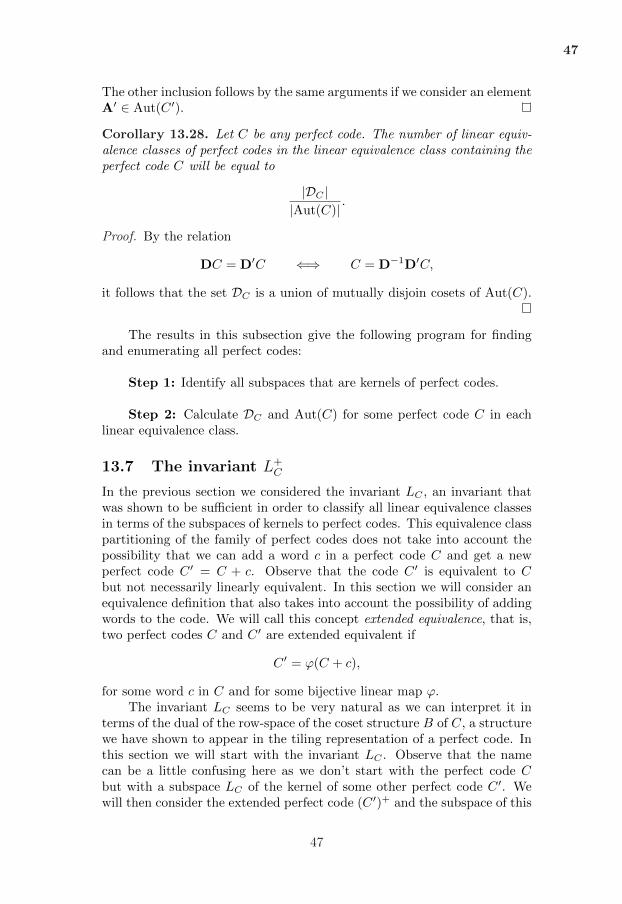
47

The other inclusion follows by the same arguments if we consider an elementA′ ∈ Aut(C ′).

Corollary 13.28. Let C be any perfect code. The number of linear equiv-alence classes of perfect codes in the linear equivalence class containing theperfect code C will be equal to

∣DC ∣∣Aut(C)∣ .

Proof. By the relation

DC = D′C ⇐⇒ C = D−1D′C,

it follows that the set DC is a union of mutually disjoin cosets of Aut(C).

The results in this subsection give the following program for findingand enumerating all perfect codes:

Step 1: Identify all subspaces that are kernels of perfect codes.

Step 2: Calculate DC and Aut(C) for some perfect code C in eachlinear equivalence class.

13.7 The invariant L+C

In the previous section we considered the invariant LC , an invariant thatwas shown to be sufficient in order to classify all linear equivalence classesin terms of the subspaces of kernels to perfect codes. This equivalence classpartitioning of the family of perfect codes does not take into account thepossibility that we can add a word c in a perfect code C and get a newperfect code C ′ = C + c. Observe that the code C ′ is equivalent to Cbut not necessarily linearly equivalent. In this section we will consider anequivalence definition that also takes into account the possibility of addingwords to the code. We will call this concept extended equivalence, that is,two perfect codes C and C ′ are extended equivalent if

C ′ = '(C + c),

for some word c in C and for some bijective linear map '.The invariant LC seems to be very natural as we can interpret it in

terms of the dual of the row-space of the coset structure B of C, a structurewe have shown to appear in the tiling representation of a perfect code. Inthis section we will start with the invariant LC . Observe that the namecan be a little confusing here as we don’t start with the perfect code Cbut with a subspace LC of the kernel of some other perfect code C ′. Wewill then consider the extended perfect code (C ′)+ and the subspace of this

47

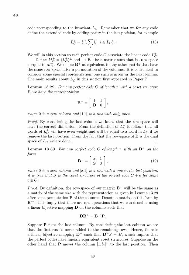
48

code corresponding to the invariant LC . Remember that we for any codedefine the extended code by adding parity in the last position, for example

L+C = {[l,

∑

i

li] ∣ l ∈ LC}. (18)

We will in this section to each perfect code C associate the linear code L+C .

Define M+C = (L+

C)⊥ and let B+ be a matrix such that its row-space

is equal to M+C . We define B+ as equivalent to any other matrix that have

the same row-space after a permutation of the columns. It is convenient toconsider some special representation; one such is given in the next lemma.The main results about L+

C in this section first appeared in Paper 7.

Lemma 13.29. For any perfect code C of length n with a coset structureB we have the representation

B+ =

[1 1B 0

],

where 0 is a zero column and [1 1] is a row with only ones.

Proof. By considering the last column we know that the row-space willhave the correct dimension. From the definition of L+

C it follows that allwords of L+

C will have even weight and will be equal to a word in LC if weremove the last position. From the fact that the row-space of B is the dualspace of LC we are done.

Lemma 13.30. For any perfect code C of length n with an B+ on theform

B+ =

[x 1S 0

], (19)

where 0 is a zero column and [x 1] is a row with a one in the last position,it is true that S is the coset structure of the perfect code C + c for somec ∈ C.

Proof. By definition, the row-space of our matrix B+ will be the same asa matrix of the same size with the representation as given in Lemma 13.29after some permutation P of the columns. Denote a matrix on this form byB+′

. This imply that there are row operations that we can describe usinga linear bijective mapping D on the columns such that

DB+ = B+′P.

Suppose P fixes the last column. By considering the last column we seethat the first row is never added to the remaining rows. Hence, there isa linear bijective mapping D− such that D−S = B, which implies thatthe perfect codes have linearly equivalent coset structures. Suppose on theother hand that P moves the column [1, bi]

T to the last position. Then

48

49

D−1 must add the all one row to all rows in which bi have the value one.Thus B is mapped to B + bi which implies that S is linearly equivalent tothe coset structure of C + c where c is contained in the coset of the kernelgiven by bi.

The two above results are more or less a proof of the following mainresult of this subsection as we always can, by a linear transformation, getthe last column on the form stipulated above, for details see below.

Theorem 13.31. Two perfect codes C and C ′ are extended equivalent ifand only if B+ and B+′

are linearly equivalent.

Proof. Suppose that the codes are extended equivalent, that is, there is aword c′ such that C and C ′ + c′ are linearly equivalent. We can then, byCorollary 13.24, assume that the coset structures are B and B + b for Cand C ′ respectively. This assumption implies that B+ is mapped to B+′

byadding the all one row to all rows where b is non-zero in the representationgiven by Lemma 13.29.

Suppose that the codes C and C ′ have linearly equivalent extendedcoset structures B+ and B+′

and hence that DB+ = B+′, for some non-

singular matrix D. Assume that

B+ =

[1 1B 0

],

as given in Lemma 13.29. The matrix D maps the columns in B+ corre-sponding to B to some of the columns in B+′

. We can assume that thesecolumns are the first columns in B+′

if we assume that B+′is on the form

given by Lemma 13.30. The result now follows from that lemma.

13.8 The natural tiling representation of a perfect code.

It was proved by Hergert [17] that the dual of the linear span of a per-fect code is a simplex code. It is easy to deduce Hergerts result from thefollowing lemma.

Lemma 13.32. For any perfect code C of length n of rank r and with akernel of dimension k, the tiling representation (A,B) can without loss ofgenerality be assumed to be such that ai = (zj , xi) for 0 ≤ i ≤ n and j isfixed for i such that 2qj − 1 ≤ i < 2q(j+1)− 1, where q = log2(n+1)−n+ rand zi ∈ Zn−r

2 is the natural binary representation of i and bi = (0n−r, yi).That is,

(A,B) =

(S , 0

A1, . . . , An , B′

), (20)

where B′ have full-rank and S is the simplex code given by the words zj ∈Zn−r2 .

49

50

Proof. From the definition of the tiling representation it follows that A isa full-rank set and that B is of dimension r − k. Hence, there is a lineartransformation such that we can get the words bi on the form as describedin this lemma. By the fact that (A,B) is a tiling we know that every word zjmust be present in the first positions of the words ai as the words bi are zeroin these positions. Further, the last r−k positions of the words with a fixedzj must give a tiling (Aj , B

′). Therefore each set Aj , for j = 1, 2, . . . , n,must be of the same cardinality and we are, by Lemma 12.1, done.

Observation 13.33. By Lemma 13.32 we can represent every perfect codeby defining sub-tilings Ai such that (zi, aj) ∈ A where aj ∈ Ai and 0 ∈ A0.Further any set of tilings (Ai, B

′) as described above gives a perfect codewith the coset structure B if we make sure that A has full rank.

The strength of the representation given by Lemma 13.32 is exemplifiedby another result that seems hard to prove. However using the abovepresented representation it will be a triviality. The next lemma was alsoproved in [13].

Lemma 13.34. Let (A,B) be any tiling with a full-rank set A and withthe associated perfect code C. Then ei ∈ ⟨C⟩ if and only if there exists dsuch that Bd = ai.

Proof. Suppose that ei ∈ ⟨C⟩. Then

ei =∑

j∈J

cj , (21)

for some minimal index set J and words cj in the code C. From thedefinition of C we get that Acj = bj , where we get a unique bj from theminimality of J (observe that the indexing of cj is a bit artificial as everybj is associated to a coset ker(C)+ cj and not specifically to the cj we pickfrom equation (21)). We conclude that

ai = Aei = A∑

j∈J

cj =∑

j∈J

Acj =∑

j∈J

bj = Bd , (22)

where d is the word with support equal to J .Suppose that Bd = ai (and remember that ai ∕= 0). Define J to be

the index set of the support of d. As A has full-rank we know that we forevery index j in J can find a cj such that Acj = bj . Either

∑j∈J cj = ei

in which case we are done or∑

j∈J cj ∕= ei. If that case we use the factthat

A

⎛⎝∑

j∈J

cj + ei

⎞⎠ = 0.

Hence we know that∑

j∈J cj+ei ∈ ker(C) and moreover that ei ∈ ⟨C⟩.

50

51

Theorem 13.35. For any perfect code C of length n and of rank r withthe tiling representation (A,B), then ei ∈ ⟨C⟩ if and only if A, such thatC = {c ∣Ac ∈ B}, has the column ai = [z0, xi]

T , z0 = 0, in position i. Asa consequence of this equivalence there is a index set I such that

∣I∣ = n+ 1

2n−r− 1,

fulfilling the conditions in the equivalence.

Proof. Suppose that we have the representation as given in Lemma 13.32,then by Lemma 13.34 we know that

I =

{1, . . . ,

n+ 1

2n−r− 1

}.

Observe that it is possible to prove Theorem 13.35 directly from thefact that the dual of a perfect code ⟨C⟩⊥ is a simplex code. The theoremthen follows by noting that all the positions corresponding to the zerocolumns in Theorem 12.1 will correspond to a word ei in the linear span ofthe code.

13.9 Phelps codes

In this section we will give the bare minimum needed to describe a class ofcodes that are called Phelps codes.

A Phelps code C = (D,Dpi,j , Q) is an extended perfect code of length

n + 1 which is defined from some other codes. There is an ”outer”-codeD which is an extended perfect code of length nO. Further for each fixedindex set {i, j, p}, where i ∈ [1, nO], j ∈ [0, nI − 1] and p ∈ [0, 1], there is atranslated (they do not necessarily contain the zero word) extended perfect”inner”-code Dp

ij . These codes are translates of extended perfect codes oflength nI = (n + 1)/nO, such that every word in such a code is of evenweight if p = 0 or of odd weight if p = 1. The ”inner codes” Dp

ij have theadditional property that for each fixed i the indices p, j give a partition ofZnI2 . The last code needed for the definition of a Phelps code is a 1-error

detecting (minimum distance 2) code Q of length nO over an alphabet withnI letters and with nnO−1

I number of words. These codes Q belong to aclass of codes called MDS-codes. These objects define the Phelps code as

C = {[c1, . . . , cnO] ∣ ci ∈ D

d(i)i,q(i) , d ∈ D , q ∈ Q}, (23)

where d(i) is position i in the word d and q(i) is position i in the word q.Observe that from the assumption 0 ∈ C it follows that 0 ∈ D. Phelps

[25] gave a more general construction, but it is not needed here. It mustbe remarked that this construction has been used in many contexts to findperfect codes with certain given prescribed properties.

51

52

13.10 FRH-codes

Let H be a Hamming code of length nH . Let CF be a full-rank perfect codeof length nH . Let T be a sub-space of H∩ker(CF ) such that the dual spaceof the row-space of a matrix T gives a coset structure B as described byTheorem 13.25. A perfect code C with a coset structure linearly equivalentto B belongs to the class of perfect codes that we call FRH-codes, whereFRH is an acronym for Full-Rank-Hamming.

The next theorem was first proved in Paper 8 and the only differencein the proof below, from the proof in that paper, is the presentation.

Theorem 13.36. Any non-full rank FRH-code C is linearly equivalent toa Phelps code.

Proof. We consider the natural tiling representation of the code C, that is,

C = (A,Be) =

(S , 0

A0, . . . , AnO−1 , B

), (24)

where S is the simplex code with zero columns in the positions associatedto the sub-tiling A0, B will be a full-rank set. Observe that if follows fromthe non-full rank condition that rank(S) ≥ 1. It remains to prove thatthere is a Phelps code linearly equivalent to this code.

Define P0 = {Bc ∣ c ∈ CF } and Pi = {Bℎ ∣ℎ ∈ H} for i ∈ [1, nO − 1].By Theorem 13.20 the pairs (Pi, B) are tilings for i ∈ [0, s]. Further, asCF and B have full-rank, it follows that P0 have full-rank. Hence, byTheorem 13.6, the code CP defined by

CP = (AP , Be) =

(S , 0

P0, . . . , PnO−1 , B

), (25)

is linearly equivalent to C.Assume, without loss of generality, that in all sets Pi the enumera-

tion of the words is such that the zero word have index 1, that is, P1 =[0, p2, . . . pnI

] and assume further that Pi = P1 if i ≥ 1. Observe that wehere assume that we have extended a code by adding parity in the firstposition (corresponding to the zero column).

We then proceed by finding a Phelps representation of the code CP

and thus proving that it is a Phelps code. For details see Paper 8.

14 Concluding remarks on perfect 1-error cor-recting binary codes

The work about perfect codes in this thesis started with a master thesis,consisting of the Papers 4-5, a master thesis that was more or less drivenby the need to do a fast enumeration of perfect codes. The master thesisstarted a work that has involved solving and trying to solve a number

52

53

of problems in this challenging and interesting field of mathematics. Theexperience from this work is that all the methods mentioned in this shortintroduction are important when working with perfect codes. Furthermore,these methods allow us to reformulate problems in a number of ways, whichis often invaluable to understand and solve the problem.

The most recent application of the methods presented here can befound in Paper 8. The main results from this article can also be foundin Subsection 13.10. That article gives the first results in the work thatI hope will give relations between some of the different constructions ofperfect codes.

Translating all results and constructions in the theory of perfect codesinto a common language seems to be an interesting problem. I believe thiswould greatly benefit the future development of the theory about perfectcodes. An example of such a problem is to give the tiling representation ofan arbitrary Phelps code.

The central (and hard problem) that would be nice to solve is theclassification of all kernels of perfect codes and to find the symmetry groupsof these kernels and their sub-spaces. This would more or less classify theperfect codes in terms of their equivalence classes and the cardinality ofthem. Another related problem, that seems to be open, is to determine ifevery kernel of a perfect code is contained in some Hamming code. If thiswere the case then the solution of many problems mentioned above wouldbe simplified.

References

[1] Aldous, D., Asymptotics in the random assignment problem, Probab.Theory Related Fields, 93 (1992) no. 4, 507–534.

[2] Aldous, D., The ³(2) limit in the random assignment problem, RandomStructures Algorithms 18 (2001), no 4. 381–418.

[3] Avgustinovich, S. V., Heden, O., F. I. Solov’eva, On perfect codesranks and kernels problem, Probl. of Inform. Transm., 39 (4) (2003),341-345.

[4] Blokhuis, A., Lam, C. W. H., More coverings by rook domains, J.Combin. Theory Ser. A, 36 (1984), 240-244.

[5] Etzion, T., Vardy, A., On perfect codes and tilings, problems and so-lutions, SIAM J. Discrete Math 11 (1998), No 2, 205-223.

[6] Frieze, A. M., On the value of a random minimum spanning tree prob-lem, Discrete Appl. Math., 10 (1985), 47–56.

[7] Gamarnik, D., Expectation of the random minimal length spanning treeof a complete graph, Proceedings of the Sixteenth Annual ACM-SIAMSymposium on Discete Algorithms (2005), 700—-704.

53

54

[8] Golay, M. J. E., Notes on Digital Coding. Proc. IRE 37 (1949), 657.

[9] Hamming, R. W., Error detecting and error correcting codes, Bell Sys-tem Technical Journal, 29 (1950), 147–160.

[10] Heden, O., Perfect codes from the dual point of view I, Discrete Math-ematics, 308 (24) (2008), 6141–6156

[11] Heden, O., A full rank perfect code of length 31, Designs, Codes andCryptygraphy 38 (1) (2006), 125–129.

[12] Heden, O., A remark on full rank perfect codes, Discrete Mathematics,306 (16) (2006), 1975–1980.

[13] Heden, O., Perfect Codes of Length n with Kernels of Dimension n-log(n + 1) - 3, to appear in Siam J. on Discrete Mathematics.

[14] Heden, O., M. Hessler, On the classification of perfect codes: Side classstructures, Designs Codes and Cryptography, 40 (2006), 319–333.

[15] Heden, O., M. Hessler, On linear equivalence and Phelps codes, sub-mitted.

[16] Heden, O., Hessler, M., Westerback, T., On the classification of perfectcodes: Extended side class structures, to appear in Discrete Mathemat-ics.

[17] Hergert, F., Algebraiche Methoden fur nichtlineare Codes, Thesis,Darmstadt 1985.

[18] Hessler, M., Perfect codes as isomorphic spaces, Discrete Mathematics,306 (16) (2006), 1981–1987.

[19] Hessler, M., A Computer study of some 1-error correcting perfect bi-nary codes, Australasian Journal of Combinatorics, 33 (2005), 217–229.

[20] Linusson, S., Wastlund, J., A proof of Parisi’s conjecture on the ran-dom assignment problem, Probab. Theory Relat. Fields 128 (2004),419–440.

[21] MacWilliams, F.J., Sloane, N.J.A., The Theory of Error-CorrectingCodes, North-Holland (1977).

[22] Nair, C., Prabhakar, B., Sharma, M., Proofs of the Parisi andCoppersmith-Sorkin random assignment conjectures, Random Struc-tures and Algorithms 27, No. 4 (2005), 413–444.

[23] Ostergard, P. R. J., Vardy, A., Resolving the existence of full-ranktilings of binary Hamming spaces, SIAM Journal on Discrete Mathe-matics 18 (2) (2004), 382-387.

54

55

[24] Parisi, G., A conjecture on random bipartite matching,arXiv:cond-mat/9801176 (1998).

[25] Phelps, K., A general product construction for error correcting codes,SIAM J. Algebraic and Discrete Methods, 5 (2) (1984), 224–228.

[26] Phelps, K. T., Villanueva, M., On perfect codes: rank and kernel,Designs, Codes and Cryptography, 27 (3) (2002), 183–194.

[27] Pless, V. S., Huffman, W.C., Brualdi, R.A., Handbook in Coding The-ory, North-Holland (1998).

[28] Shapiro, G. S., Slotnik, D. S., On the mathematical theory of errorcorrecting codes, IBM Journal of Research Development 3 (1959), 68-72.

[29] Solov’eva, F. I., On Perfect Codes and Related Topics, Com2Mac Lec-ture Note Series 13, Pohang 2004.

[30] Trachtenberg, A., Vardy, A., Full-Rank tilings of F 82 do not exist,

SIAM Journal on Discrete Mathematics, Volume 16 (3) (2003), 390-392.

[31] Vasil’ev, Y. L., On nongroup close-packed codes, Problems of Cyber-netics, 8 (1962), 375-378.

[32] Whitney, H., On the abstract properties of linear dependence, Ameri-can Journal of Mathematics 57 (1935), 509-533.

[33] Zinoviev, V. A., Zinoviev, D. V., Binary perfect codes of length 15by generalized concatenation construction, Problems of InformationTransmission, 39 (1) (2003), 27–39.

55