Optimization of Algorithms for Mobility in Cellular Systems

Op

timizatio

n o

f Alg

orith

ms fo

r Mo

bility in

Cellu

lar Systems

Department of Electrical and Information Technology, Faculty of Engineering, LTH, Lund University, 2016.

Optimization of Algorithms forMobility in Cellular Systems

Bernt ChristensenOlof Knape

Series of Master’s thesesDepartment of Electrical and Information Technology

LU/LTH-EIT 2016-509

http://www.eit.lth.se

Be

rnt C

hriste

nse

n &

Olo

f Kn

ap

e

Master’s Thesis

Optimization of algorithms for mobility in

cellular systems

Bernt Christensen

[email protected] Knape

[email protected]

June 8, 2016

Master’s thesis work in electrical and information technology carried out

at Ericsson AB.

Supervisors: Niklas Holmqvist, [email protected] Wichert, [email protected]

Fredrik Tufvesson, [email protected]

Examiner: Fredrik Rusek, [email protected]

Abstract

Inter-frequency measurements are needed to determine when user equipment

should make a handover to the best available base station in a cellular mobile

network. The measurements are expensive from a resource point of view and

therefore there is a need for optimization of this kind of measurements. In

this work both this optimization and a way to predict the future of the mea-

surements have been evaluated in a simulated Long-Term Evolution network.

Both fast and slowly moving user equipment have been tested and the predic-

tion was made by storing old measurements and calculating the gradient of the

signal power. Depending on the resulting signal’s gradient, different decisions

on what to do were made. The results were then compared to the traditional

way of controlling the inter-frequency measurements, in terms of throughput,

handover failures and other quality factors.

The results from the simulations show that there is some optimization that

can be made without compromising the connection. More specifically, the

time spent measuring inter-frequency has been successfully improved (low-

ered). Handover failures have been harder to control and the throughput has

more or less been unchanged throughout the simulations. The speed of the

user equipment influenced the results a lot and no setup was found that works

best with all UE speeds.

Keywords: Handover, Long-Term Evolution, UE speed, measurement optimization,

inter-frequency measurement, prediction, simulation

2

Acknowledgements

We would like to thank Fredrik Tufvesson at LTH for his important feedback and advice.

We would also like to thank Niklas Holmqvist and JanWichert for the opportunity to work

with this thesis at Ericsson and for their invaluable help and feedback throughout the work.

At last we would also like to thank Niclas Palm and Staffan Haglund for their guidance in

the technical details of the used simulator.

3

4

Abbreviations

33G - Third Generation of mobile telecommunications technology

3GPP - 3rd Generation Partnership Project

BBS - Base Station

BTS - Base Transceiver Station

EE-UTRA - Evolved UMTS Terrestrial Radio Access

E-UTRAN - Evolved UMTS Terrestrial Radio Access Network

eNB - evolved Node B

GGSM - Global System for Mobile Communications (originally Groupe Spécial Mobile)

HHO - Handover

HOF - Handover Failure

Hys - Hysteresis

LLTE - Long-Term Evolution

PPCell - Primary Cell

PSCell - Primary Secondary Cell

QQoS - Quality of Service

5

RRLF - Radio Link Failure

RS-SINR - Reference Signal - Signal to Interference and Noise Ratio

RSRP - Reference Signal Received Power

RSRQ - Reference Signal Received Quality

RSSI - Received Signal Strength Indicator

SSCell - Secondary Cell

SINR - Signal to Interference and Noise Ratio

SON - Self-Organizing Network

TTTT - Time To Trigger

UUE - User Equipment

UMTS - Universal Mobile Telecommunications System

6

Contents

1 Introduction 91.1 Background . . . . . . . . . . . . . . . . . . . . . . . . . . . . . . . . . 9

1.2 Problem Statements . . . . . . . . . . . . . . . . . . . . . . . . . . . . . 9

1.3 Purpose . . . . . . . . . . . . . . . . . . . . . . . . . . . . . . . . . . . 10

1.4 Method . . . . . . . . . . . . . . . . . . . . . . . . . . . . . . . . . . . 10

1.5 Scope . . . . . . . . . . . . . . . . . . . . . . . . . . . . . . . . . . . . 10

1.6 Report Layout . . . . . . . . . . . . . . . . . . . . . . . . . . . . . . . . 11

2 Theory 132.1 Cellular Networks . . . . . . . . . . . . . . . . . . . . . . . . . . . . . . 13

2.2 Measurements . . . . . . . . . . . . . . . . . . . . . . . . . . . . . . . . 14

2.3 Handovers . . . . . . . . . . . . . . . . . . . . . . . . . . . . . . . . . . 15

2.3.1 Handover events . . . . . . . . . . . . . . . . . . . . . . . . . . 16

2.3.2 Handover failures . . . . . . . . . . . . . . . . . . . . . . . . . . 19

2.4 Self-Organizing Networks . . . . . . . . . . . . . . . . . . . . . . . . . 22

2.5 Quality of Service . . . . . . . . . . . . . . . . . . . . . . . . . . . . . . 22

3 System Description 233.1 Environment . . . . . . . . . . . . . . . . . . . . . . . . . . . . . . . . . 23

3.2 Event procedures . . . . . . . . . . . . . . . . . . . . . . . . . . . . . . 25

4 Experiments 314.1 Simulation 1 - Environment evaluation . . . . . . . . . . . . . . . . . . . 31

4.2 Simulation 2 - Negative gradient . . . . . . . . . . . . . . . . . . . . . . 31

4.3 Simulation 3 - Positive gradient . . . . . . . . . . . . . . . . . . . . . . . 34

4.4 Simulation 4 - Gradients combined . . . . . . . . . . . . . . . . . . . . . 35

4.5 Simulation 5 - Worst case gradient . . . . . . . . . . . . . . . . . . . . . 35

5 Results 375.1 Simulation 1 - Environment evaluation . . . . . . . . . . . . . . . . . . . 37


7

CONTENTS




6 Analysis 576.1 Simulation 1 - Environment evaluation . . . . . . . . . . . . . . . . . . . 57


6.2.1 UE speed 3 km/h . . . . . . . . . . . . . . . . . . . . . . . . . . 58

6.2.2 UE speed 30 km/h . . . . . . . . . . . . . . . . . . . . . . . . . 58

6.2.3 UE speed 120 km/h . . . . . . . . . . . . . . . . . . . . . . . . . 58

6.2.4 UE speed 350 km/h . . . . . . . . . . . . . . . . . . . . . . . . . 59




6.6 Summary . . . . . . . . . . . . . . . . . . . . . . . . . . . . . . . . . . 61

7 Discussion 637.1 The environment . . . . . . . . . . . . . . . . . . . . . . . . . . . . . . 63

7.2 The results . . . . . . . . . . . . . . . . . . . . . . . . . . . . . . . . . . 64

7.3 Other aspects . . . . . . . . . . . . . . . . . . . . . . . . . . . . . . . . 65

8 Conclusions 67

9 Future Work 69

Bibliography 71

8

Chapter 1Introduction

1.1 BackgroundWith a growing number of connected users and an increasing amount of traffic in the

mobile network, there is an increasing demand on the availability, performance and quality

of the network. The usage of different kinds of streaming services is increasing which

requires better throughput but also requires the connection to be more stable and available

at all times. At the same time there are limitations on the throughput and how many users

there can be within a certain area and still provide good service to all of those users.

Therefore it is very important that the load of the network is distributed within the network

and that each user is provided with a good connection, based on the user’s location. This

may sound like an easy task but the fact that the users are moving with various moving

patterns and at various speeds makes it harder. Therefore it is important to implement

sophisticated algorithms that can estimate a user’s movement and be optimized to give the

best service possible to the users. At the same time there are limitations on the processing

power and what data that can be retrieved from the users, because of the limitations of the

user equipment (UE, e.g., a mobile phone or a tablet). Therefore it would be preferable to

do as small amount of measurements and calculations as possible without impairing the

service and making incorrect mobility decisions.

1.2 Problem StatementsIn the thesis we study the following problems:

1. Is it possible for the UE in the simulator to find the current signal quality’s rate of

change, based on its measurements?

2. Based on the rate of change, is it possible to predict when a handover (HO) should

be made (both initiated and finished)?

9

1. Introduction

3. Will this new way be more efficient than current solution, in terms of calculation

effort and measurement effort without compromising the Quality of Service (QoS)?

1.3 PurposeThe purpose was to try to find answers to the questions stated in Section 1.2 and by doing

so, find a new way to analyze measurements made by the UE. Based on the analysis, which

takes the rate of change in signal quality into account, the UE might be able to reduce the

number of measurements needed to make a good estimation for when a HO should be

made without an unacceptable increase in calculation effort.

1.4 MethodThe thesis work was divided into two parts; the first method used was a literature study

and the second was experiments using simulations to find whether or not the suggested

algorithm gave better performance.

The literature study was used to find research to base this work on. Literature was

searched for using Lund University’s search engine, LUBsearch and IEEE Explore where

keywords such as handover, speed, measurement and prediction was used. Once such

searches have been made, references in the found papers lead to further papers and refer-

ences. For documentation regarding the standardization of the technology the homepage

of the 3rd Generation Partnership Project (3GPP) has been used. 3GPP is a partnership

organization that unites seven telecommunications standard development organizations

which together provides and develops the mobile broadband standard.

In the second part experiments were used by simulating both the previous procedure

and the new suggested procedure, using an algorithm, both using the same environment.

This was used to be able to do a comparison between the performance in the old way and

the suggested way of doing this. More on how the simulation was setup is described in

Chapter 3.

1.5 ScopeAlthough there are several different telecommunication technologies in use today this

study only took Long-Term Evolution (LTE) under consideration. The study was also

limited to making simulations with a simulator provided by Ericsson. All the limits that

came with the simulator were also limitations to this work. There was no end to the num-

ber of cell deployments available, neither in reality or in the simulator, but it was chosen to

limit this study to the usage of 3GPP case 1 and case 3, these are described in Chapter 3.1.

The study considered connected UEs, which means that UEs in an idling state were

excluded. The UE is in a connected state when some kind of transfer is ongoing between

the UE and the base station (BS), this can be, e.g., a phone call or data transfer due to

sending or receiving an E-mail.

The study only took measurements in the UE in consideration and left out the mea-

surements made by the BS. The intra-frequency measurements were also left out of this

10

1.6 Report Layout

work, the focus was on inter-frequency measurements. There are different ways to mea-

sure the signal power/quality between the UE and the BS, this study was limited to the

usage of Reference Signal Received Power (RSRP). The concepts and ideas in this thesis

could relatively easily be tried with other measurement units than RSRP. The scope was

also limited to the measurements preceding the actual HO, meaning that the study focused

on when the HO was made and did not look into the details of how the UE chose target

cell or how the HO was made. The result of the HO, if it should succeed or fail, was an

important aspect and was taken into account for the end result of the study.

1.6 Report LayoutThe first chapter of the report gives an introduction to the area and the problem which was

tried to solve. Chapter 2 describes the theory needed to understand the area and goes a

bit more into details. After this, Chapter 3 gives a description on how the simulation was

setup and why. Chapter 4 describes the different simulations made. In Chapter 5 the result

from each of the simulations is presented. Chapter 6 analyzes the results from each of the

separate simulations. The total outcome of the results and the analysis are discussed in

Chapter 7 and concluded in Chapter 8. Lastly future work related to this work is suggested

in Chapter 9.

11

1. Introduction

12

Chapter 2Theory

This chapter gives the theoretical background this thesis is built upon. The chapter begins

with an overview of cellular networks and explains the different measurements made and

why they are important. After this follows a detailed description of HOs and then follows

an overview of Self-Organizing Networks which in a way explains the motivation behind

this thesis. The chapter ends with an explanation of what factors of QoS that are studied

in this thesis.

2.1 Cellular NetworksThe radio access network (later referred to as network) that provides UEs with connectivity

is divided into several parts. The complete network is composed of many BSs that each has

a cell site, a geographical area in which the BS provides connectivity. This site in turn is

divided into one or more cells. Each cell uses one frequency interval through which the UE

and the BS communicates. Cells with different frequency intervals might cover the same

area to provide service to more UEs within that area. Each UE is normally connected to

one of these cells in order to be able to use any of the features provided from the phone

service provider, e.g., making a voice call or surfing on the Internet.

There are several different sizes of the cells. The largest is covered by a macro BS,

within 3GPP categorized as ’wide area BS’ and is often used as the base in a network

deployment. They use a relatively high transmit power (20-40 W) and the antennas are

usually located above roof-top level. Then there is the micro BS that is located below roof-

top level and is often limited by neighboring buildings. Micro BS is specified ’medium

range BS’ in 3GPP and is using 5-10 W. Pico BS is referred to as ’local area BS’ in 3GPP

and transmits using 0.25 W at most. They cover a small area but still bigger than a femto

BS which is intended to use in a small office or at home and is called ’home BS’ in 3GPP.

It uses 0.1 W at most and differs from the rest by usually being connected to the network

through a home broadband connection to a femto gateway [1]. Take notice that the cells

13

2. Theory

does not always align next to each other covering different areas, they often overlap. There

could also be a cell within the area of a bigger cell, e.g., a femto cell could be within the

area of a macro cell [1][2].

The BS in different network solutions is called different things, in LTE which is the fo-

cus in this thesis, the BS is called evolved Node B (eNB) while, e.g., within Global System

for Mobile Communications (GSM) the BS is called base transceiver station (BTS). The

network itself is also called different things, in LTE the network is called Evolved UMTS

Terrestrial Radio Access Network (E-UTRAN) and Evolved UMTS Terrestrial Radio Ac-

cess (E-UTRA) refers to the interface in use. Where Universal Mobile Telecommunica-

tions System (UMTS) is the name of a technology used in the third generation of mobile

telecommunications technology (3G). The focus of this thesis is LTE and therefore, from

now on, the names and expressions connected to LTE will be used.

The Figure 2.1 below illustrates an example on how an E-UTRAN could look, with

eNBs with different number of cells and different cell sizes. There are also some UEs

placed in the cells.

Figure 2.1: An example of an E-UTRAN. Each color represents

an eNB and its cells.

2.2 MeasurementsA connected UE is continuously makingmeasurements against the cells in the surrounding

area in order to find the cell which provides the best service/coverage available to the UE.

The measurements are made by monitoring reference signals sent out from the cells. How

the measurements should be done is configured by the eNB and this specification can cover

how often the measurement are made, what to measure and when to send measurement

reports to the eNB. The reports can be configured to be sent within different time intervals

14

2.3 Handovers

or based on defined events, e.g., the UE measures a value lower than a defined threshold

value [1][3]. There are several values that can be measured and used to determine which

cell to be connected to, what to measure depends on the configuration for that cell [1].

Themost basic measurement that could be monitored is the RSRP. RSRP is the average

power received from a single cell specific reference signal resource element, measured in

watts. In other words, the RSRP provides ameasurement of the signal strength between the

UE and the cell, measured in the UE [1]. RSRP takes the signal’s power in consideration,

not the signal’s quality. Therefore there is also Reference Signal Received Quality (RSRQ)

that states the signals quality by taking the other interfering signals under consideration.

RSRQ is defined as

N ∗ RSRPRSSI

= RSRQ,

where N is the number of Resource Blocks and Received Signal Strength Indicator (RSSI)

is the average received total power from the serving cell, other cells and noise from other

sources [1][3]. The serving cell refers to all the cells that provides a connection to the

UE and consists of the primary cell (PCell) and the secondary cells (SCell). Where PCell

refers to the cell that operates on the primary frequency to which the UE performs ini-

tial connection and re-establishment. The primary secondary cell (PSCell) has the same

responsibility as the primary cell but for the secondary cells, that operates on a second

frequency.

Another type of measurement that describes the quality of the signal is signal to noise

and interference ratio (SINR) and is defined as

SINR =S

I + N,

where S is the power of the usable measured signals, I is the average interference power

and N is the noise power [3][4].

There are two different ways for the UE to find cells in the area, one is using intra-

frequencymeasurements and the other is inter-frequencymeasurements. The intra-frequency

measurements are made by measuring against the neighboring cells using the same fre-

quency currently used between the UE and the serving cell. The other, inter-frequency

measurements are made against the cells within transmission gaps. During these gaps the

UE retune the receiver to monitor other frequencies, makes the measurements and then

goes back to the original frequency again [5][6]. Due to the fact that there cannot be

any regular transmissions between the UE and the serving cell during the inter-frequency

measurements these are considered costly in terms of resources used and therefore intra-

frequency measurements are preferred where the measurements do not cause a transmis-

sion gap [5].

2.3 HandoversWhen a UE is moving from one cell to another the connection to the cell needs to be

transferred from the old cell to the new one. This can be done by either a HO or a cell

reselection. A HO refers to a transfer between two cells while the UE is active (connected)

in either a voice call or some other kind of data transfer. A reselection is while the UE is

15

2. Theory

in idle mode which means that there is no transfer going on but the UE is still monitoring

incoming calls [7].

Usually the UE does a HO or a reselection from the serving cell to the target cell,

depending on where the best QoS can be delivered to the UE. QoS in this case refers to

which degree of satisfaction a user has for the service, which include different aspects

of performance: operability-, accessibility-, retainability- and integrity- performance [8].

From a UE point of view a more specific interpretation of QoS can be found in Section 2.5.

The QoS is determined by looking at the different measurements described in Section 2.2.

The user would probably not notice if something goes wrong during a reselection since

there is no active transmission going on to the UE. On the other hand, if something goes

wrong during a HO, delay-sensitive data transmissions could be interrupted causing, e.g.,

a broken phone call. Therefore it is more important that the HO procedure is made without

complications than the procedure of a reselection. For this reason HO will be in focus of

this work.

An unintended loss of the connection between the UE and the cell is called a Radio

Link Failure (RLF). This might happen if the connection to the serving cell is lost before

a new target cell is ready to establish a connection to the UE.

A HO can be made in three different ways [9][10]:

1. Hard HO, where the current connection between the UE and the serving cell is bro-

ken down before a new connection to the target cell is established.

2. Soft HO refers to a scenario where the new connection is established before the

current is broken. More specifically soft HO only refers to a HO between two cells

with different BSs. The UE consumes double amount of bandwidth in a soft HO

compared to a hard HO, because it is connected to two cells during the HO.

3. Softer HO is almost the same as soft HO, but softer refers to a HO between two cells

of the same BS. Naturally the UE consumes double amount of resources in a softer

HO compared to a hard HO as well.

In LTE there is only hard HO in use, mainly because of the complexity and the waste

of resources in soft and softer HO [1]. Therefore hard HO is the focus for the simulations

and as of now hard HO is what is meant by HO if nothing else is stated. Because hard HO

is the focus this also means that the estimation of when the HO should be made is even

more important because the connection is broken before a new connection is established.

Another important aspect of the HO is if the HO is intra- or inter-frequency. As men-

tioned in Section 2.2 the UE can search for cells on different frequencies than the one

currently used communicating with the serving cell. These HOs to other frequencies are

called inter-frequency HOs. HOs within the same frequency are called intra-frequency

HOs.

2.3.1 Handover eventsThe UE measures the RSRP periodically and takes action on these measurements when

the events below occur. There are six defined events within LTE that can be used to decide

when the UE should take action. Each event has at least one entering condition and one

16

2.3 Handovers

leaving condition, these conditions defines when the event starts and ends. The six defined

HO events are the following [7]:

Event A1The A1 event occurs when the signal measurement of the serving cell becomes better than

a certain threshold and the hysteresis (Hys) combined. The same event is left when the

measurement of the serving cell combined with the Hys becomes worse than the same

threshold. An example of the entry and exit of an A1 event can be seen in Figure 3.2 and

the entering condition is defined as

Ms − Hys > Thresh

and the leaving condition is defined as

Ms + Hys < Thresh,

where Ms is the value of the serving cell measured in dBm if RSRP is used or in dB in

case of RSRQ and Reference Signal - Signal to Interference and Noise Ratio (RS-SINR).

Hys is the hysteresis expressed in dB and Thresh is the threshold measured in the same

unit as Ms.

Event A2When the measurement of the serving cell and Hys combined becomes worse than the

threshold an A2 event is entered. When the serving cell measurement is better than the

Hys and threshold combined the leaving condition is fulfilled and the event is left. This

can be seen in Figure 3.3 and the entering condition is defined as

Ms + Hys < Thresh


Ms − Hys > Thresh,

where Ms is the value of the serving cell measured in dBm if RSRP is used or in dB in case

of RSRQ and RS-SINR. Hys is the hysteresis expressed in dB and Thresh is the desired

threshold measured in the same unit as Ms.

Event A3When a neighboring cell becomes (offset, a value) better than the serving cell and Hyscombined the A3 event’s entering condition is met and the event is entered. If the neigh-

boring cell, offset and Hys combined becomes worse than the serving cell with its offset

the event is left, as the leaving condition is met. The entering condition is defined as

Mn + Of n + Ocn − Hys > Mp + Of p + Ocp + Of f


Mn + Of n + Ocn + Hys < Mp + Of p + Ocp + Of f ,

17

2. Theory

where Mn is the measurements of the neighboring cell, measured in dBm if RSRP is used

or in dB in case of RSRQ and RS-SINR. Of n is the frequency specific offset and Ocn the

cell specific offset, both of the neighbor cell, expressed in dB. Mp is the measurement

of the PCell/PSCell, measured in dBm if RSRP is used or in dB in case of RSRQ and

RS-SINR. Of p is the frequency specific offset and Ocp the cell specific offset, both of the

PCell/PSCell, expressed in dB. Off is the offset parameter for the event and is expressed

in dB. In the Figure 3.4 where an A3 event can be seen, the event offset is the only offset

used.

Event A4An A4 event is entered when a neighboring cell becomes better than threshold and Hyscombined. The event is left when the neighboring cell and Hys combined are worse than

the threshold. The entering condition is defined as

Mn + Of n + Ocn − Hys > Thresh


Mn + Of n + Ocn + Hys < Thresh,

where Mn is the measurements of the neighboring cell, measured in dBm if RSRP is used

or in dB in case of RSRQ andRS-SINR.Of n is the frequency specific offset andOcn the cell

specific offset, both of the neighbor cell, expressed in dB. Hys is the hysteresis expressedin dB and Thresh is the threshold measured in the same unit as Mn.

Event A5An A5 event is entered when two entering conditions are fulfilled. First the serving cell

and Hys combined become lower than the first threshold and secondly the neighboring cell

becomes higher than a second threshold and Hys combined. An A2 event followed by an

A5 event can be seen in Figure 3.5. The A5 event is left if either serving cell becomes

higher than the sum of the first threshold and Hys or if the sum of the neighboring cell and

Hys becomes lower than the second threshold. The entering conditions are defined as

Mp + Hys < Thresh1

and

Mn + Of n + Ocn − Hys > Thresh2

and the leaving conditions are defined as

Mp − Hys > Thresh1

and

Mn + Of n + Ocn + Hys < Thresh2,

where Mp is the measurement of the PCell/PSCell and Mn is the measurements of the

neighboring cell, both measured in dBm if RSRP is used or in dB in case of RSRQ and

RS-SINR. Of n is the frequency specific offset and Ocn the cell specific offset, both of the

neighbor cell, expressed in dB. Hys is the hysteresis expressed in dB. Thresh1 is the first

threshold and is expressed in the same unit as Mp and Thresh2 is the second threshold and

is expressed in the same unit as Mn.

18

2.3 Handovers

Event A6When a neighboring cell’s measurement become higher than the sum of the serving cell’s

measurement, the offset and the Hys, an A6 event is entered. If the sum of the same

neighboring cell’s measurement and the Hys becomes lower than the sum of the serving

cell’s measurement and the offset, the leaving condition is fulfilled and the event is left.

The entering condition is defined as

Mn + Ocn − Hys > Ms + Ocs + Of f


Mn + Ocn + Hys < Ms + Ocs + Of f ,

where Mn is the measurements of the neighboring cell and Ms is the measurement of

the serving cell, both measured in dBm if RSRP is used or in dB in case of RSRQ and

RS-SINR. Ocn us the cell specific offset of the neighbor cell, expressed in dB. Hys is thehysteresis expressed in dB. Ocs is the cell specific offset of the serving cell and is expressed

in dB. Off is the offset parameter for the event and is expressed in dB.

General parametersTime to trigger (TTT) is another important parameter for these events. Time to trigger

is the time the enter condition of the event must be fulfilled before the UE takes action.

Since the actions should not be based on too temporary conditions this is important. But

at the same time a too long time to trigger can lead to decisions being taken too late by

the UE. What action to take is configurable but the entering of an event always results in

a measurement report sent by the UE to the eNB to inform the eNB of the status of the

UE. Besides sending the measurement report the event can also trigger a HO-request or

starting/stopping inter-frequency measurements [1].

Offsets are used rather widely within this area and can sometimes be seen as a kind of

safety margin, e.g., when a HO should be made without resulting in a radio link failure.

The cell can also add an offset to the measurement result in case the cell is heavy loaded

as a kind of load balancing. This way the well populated cells can spread their UEs to

adjacent cells.

The UE does not make any difference in which eNBs that are available, the only thing

that matters is what cells are found and if they are better than current cell. The UE can

choose to make a HO to a different cell at the same eNB or to another eNB, the only thing

that matters are the results of the measurements and which events (A1-A6) they trigger.

2.3.2 Handover failuresWhenever a HO decision is wrong there is a big risk that the HO process will result in

a Handover failure (HOF). When that happens the UE chooses to either reconnect to the

previous serving cell or to another neighboring cell. In LTE there are three different HOF

[11][12][13][14]:

19

2. Theory

Figure 2.2: A too early HO. The arrow from the UE represents

the UE’s moving pattern, the x represents radio link failure and

the red dot represents a HO.

1. Too early HO usually happens when the value of time to trigger is too low. The

HO happens to early and could possibly result in a radio link failure if not the UE

performs a HO back to original cell. This procedure can be seen in Figure 2.2.

2. Too late HO usually happens when the value of time to trigger is too high. The HO

happens too late and results in a radio link failure. This procedure can be seen in

Figure 2.3.

Figure 2.3: A too late HO. The arrow from the UE represents the

UE’s moving pattern, the x represents a radio link failure.

3. HO to wrong cell involves three cells: the serving cell, the targeted cell and the

reconnecting cell. The UE performs a HO to the target cell from the serving cell but

it results in radio link failure and the UE reconnects to the third cell. This procedure

can be seen in Figure 2.4.

These three are the HOF that can result in a radio link failure but because a HO is

20

2.3 Handovers

Figure 2.4: A HO to the wrong cell. The arrow from the UE

represents the UE’s moving pattern, the x represents a radio link

failure and the red dot represents a HO.

resource consuming it is desired to avoid another problem called Ping-Pong HO. The Ping-

Pong HO happens when a UE moves near the edge of a eNB which can cause a lot of

back and forth HO between the serving cell and neighboring cells [11][12][13][14]. See

Figure 2.5.

Figure 2.5: Ping-Pong HO. The arrow from the UE represents the

UE’s moving pattern, the red dot represents a HO.

21

2. Theory

2.4 Self-Organizing NetworksAs the size and complexity of cellular networks such as LTE increases, it is more challeng-

ing to handle deployment and maintenance. Therefore there is a need for a network that

can configure and maintain itself, a network like that is called Self-Organizing Network

(SON). SON consists of three different processes [1][14]:

1. Self-configuration, which is the networks ability to automatically configure a newly

deployed cell to fit into the existing network.

2. Self-optimization, which is when the eNB’s and the UE’s measurements are used for

optimizing the configurations automatically to improve the network performance.

3. Self-healing, which refers to the networks ability to detect fault, diagnose fault and

to recover from fault.

The self-optimization component uses, among other things, optimization of the HOs

by configuring the parameters in the different events (A1-A6) described in Section 2.3

[14]. This is also the component the authors are trying to improve; a better estimation of

when the HO should be made that are based on the measurements of the UE, will lead to

better self-optimization.

2.5 Quality of ServiceAs stated in problem statement 3 in Chapter 1.2 QoS factors from a UE point of view are

used to evaluate the results. The QoS factors that are considered in this work are:

• The downlink throughput, a measurement made by the UE of how much data it can

receive, which should be at its highest at all times.

• HOF, when a HO goes wrong and the connection is lost. It is not desirable as the UE

cannot send or retrieve data during a HOF and must also reestablish the connection.

This influences the throughput and signaling load in a negative way.

• Inter-frequency measurements, time spent measuring inter-frequency. This is con-

nected to problem statement 3 in Chapter 1.2. The goal is to lower the time spent

because during this time there cannot be any regular transmissions between the UE

and the eNB.

• Late A2 measurement reports, reports that arrive later than the time needed to pre-

pare for an inter-frequency HO. The authors believe this is important because the

number of late A2 measurements reports is strongly correlated to HOFs. More de-

tails about late A2 measurements reports can be found in Chapter 4.2.

These four factors were measured and reviewed after each of the simulations and rep-

resented the quality factors that we aim to improve. Except for these four factors there

were two other things that were measured during the simulations: number of HOs and

triggered events. These were not the most important factors but a big increase of HOs was

not desirable as the procedure is time consuming and no regular transmissions between

the UE and eNB can be made during this time.

22

Chapter 3System Description

In this chapter the simulation environment is described both in terms of cell deployment

and how the different events are used. The parameters that change between the different

experiments are described later on in Chapter 4 where the experiments are described.

3.1 EnvironmentThe chosen simulation environment is defined and used within 3GPP with the purpose to

resemble different common scenarios from reality. The cell deployments as a whole is

far from the reality, but functions as a good environment for a study such as this thesis.

More specifically two different macro-cell deployments have been chosen which are called

case 1 and case 3. Case 1 represents a deployment where the distance between the sites

are 500 m. Case 3 have a distance of 1732 m between the sites (inter-cell distance) [15].

The cell deployments have 7 sites each and each site has 3 sectors. Each sector has 2

macro-cells which uses one carrier frequency each, 2.14 GHz and 0.88 GHz. This results

in a total of 42 cells and an overview of case 1 and case 3 is seen in Table 3.1.

Table 3.1: Features of the cell deployment in case 1 and case 3.

Cell deployment - Case 1 / Case 3Inter-Cell Distance 500 m / 1732 m

Number of sites 7

Sectors per site 3

Cells per sector 2

Total number of cells 42

Carrier frequency 2.14 GHz & 0.88 GHz

In case 1 and case 3 the speed of the UE was specified to 3 km/h but since different

speeds were essential for the evaluation in this thesis, the speeds 3, 30, 120 and 350 km/h

23

3. System Description

have been chosen. These speeds have been established as standard speeds when testing

mobility by 3GPP [16]. The speed of the UE changed between the different iterations of

the simulation but within the iteration the speed remained the same for all of the UEs. The

UEs move in a straight line with a random start location and direction. The first connection

the UEs does is always to a cell with a carrier frequency of 2.14 GHz, the reason for this is

to create scenarios where inter-frequency HOs are favorable. This is based on the fact that

a high frequency signal does not propagate as good as a low frequency signal and therefore

an inter-frequency HO can offer the UE a better cell as they move away from the sector.

An example of a newly connected UE and its HOs can be seen in Figure 3.1.

Figure 3.1: The environment contains two frequencies, the low

frequency reaches longer than the high. When the UE is mov-

ing it makes two HOs, the first red dot shows an inter-frequency

HO (from high to low) and the second dot an intra-frequency HO

(within low).

The simulations run for 40.5 seconds and in each simulation there are 30 UEs mov-

ing around. The reason for using a relatively small amount of UEs is to avoid possible

interference between the UEs. The interference could influence the results in undesired

ways which is not related to the algorithm itself. Therefore to ensure that enough data is

provided to create statistical significance, each simulation runs with 100 different seeds.

In conclusion, there are four iterations for each simulation where the speed of the UE is

varied, each of the iterations have 30 UEs and run with 100 different random seeds. This

results in data from 3000 UEs for each of the iterations and 12000 UEs for each simulation.

An overview of the general settings used by all simulations (if nothing else is stated) can

be seen in Table 3.2.

Table 3.2: Settings used by all simulations.

General settingsSimulation time 40.5 s

Seeds per iteration 100

UEs per iteration 30

UE speeds 3, 30, 120, 350 km/h

24

3.2 Event procedures

3.2 Event proceduresAs mentioned in Section 2.3.1 there are some events defined to determine what action the

UE should take, which are configurable. The configuration that is used in the simulations

can be seen in Table 3.3.

Table 3.3: Event settings.

Event SettingsA1 Deactivate inter-frequency measurements

A2 Activate inter-frequency measurements

A3 Intra-frequency HO

A4 Not used

A5 Inter-frequency HO

A6 Not used

In this configuration some of the events are dependent on other events and some are

independent. An A1 event can only trigger after an A2 event, because otherwise there is no

inter-frequency measurements to deactivate. After an A1 event has triggered the A2 event

can trigger again. An A5 event can also only trigger after an A2 event because the inter-

frequency measurements are needed to fulfill the entering conditions of A5. Examples of

each event procedure can be seen in the Figures 3.2, 3.3, 3.4 and 3.5. Take notice of that

Figure 3.5 contains both an A5 event and an A2 event because of their important relation.

The thresholds, Hys and time to trigger for the events are configurable. The values for

each of the parameters used in the simulations are shown in Table 3.4. The A5 threshold

has been chosen based on the number of HOFs, which should be as low as possible. A

lower threshold give a lower amount of inter-frequency measurements, which is a goal, but

this also come with a higher number of HOFs, which is not desirable. The other thresholds

have been chosen to fit together with the A5 threshold.

Table 3.4: Parameters related to the events and their values.

Event Threshold (dB) Hysteresis (dB) Time To Trigger (s)A1 -95 1 0.04

A2 -105 1 0.04

A3 31 1 0.04

A5 -110, -1002 2 0.041 The offset between serving cell and best cell.2 Serving cell threshold and best inter-frequency cell threshold.

25


Figure 3.2: An example of an A1 event. The line represents the

serving cells RSRP over time. Entering an A1 event occurs when

the RSRP-value is greater than the specified threshold and Hys

combined for a time period of time to trigger (TTT). Leaving the

same event occurs instantly when a RSRP-value is Hys lower than

the threshold.

26


Figure 3.3: An example of an A2 event. The line represents the

serving cells RSRP over time. Entering an A2 event occurs when

the RSRP-value is lower than the specified threshold andHys com-

bined for a time period of time to trigger (TTT). Leaving the same

event occurs instantly when a RSRP-value is Hys greater than the

threshold.

27


Figure 3.4: An example of an A3 event that results in a HO. The

two lines represent two different cells RSRP over time. The bold

line indicates if the cell is serving or not. The event occurs when

the serving cell is offset and Hys combined lower than the best

available cell with the same carrier frequency during the time pe-

riod of time to trigger (TTT). When the event is triggered an intra-

frequency HO is made.

28


Figure 3.5: An example of an A2 event followed by an A5 event

and a HO. The two lines represent two different cells RSRP over

time. The bold line indicates if the cell is serving or not. The A2

event occurs and starts the inter-frequency measurements. An A5

event occurs when both entering conditions are satisfied for the

duration of the time to trigger (TTT) time interval which results in

an inter-frequency HO.

29


30

Chapter 4Experiments

In this chapter the different simulations of the experiment are described more in detail with

the different settings used.

4.1 Simulation 1 - Environment evaluationIn the first simulation the environment was evaluated to see if the inter-frequency measure-

ments and HOs were used. The measurements looking for A1, A2 and A5 were turned off

and compared to a simulation where they remained turned on. The environments evalu-

ated were case 1 and case 3, as described in Section 3.1. Usually the simulations used 100

seeds to gain enough data but simulation 1 only used 10 seeds. The reason for this was

that simulation 1 only was a small study of case 1 and case 3 to gain knowledge about the

chosen cell deployments relation to inter-frequency measurements and HOs, therefore 10

seeds was sufficient in this case.

4.2 Simulation 2 - Negative gradientDuring the simulations the main goal is to discover if it is possible at all in the simulator

to find the gradient of the change in signal measured by the UE. This would be achieved

by saving previous measurements and take one of those made measurements, not too far

back in the history and calculate the difference between that measurement and the latest

measurement. This result is divided by the difference in time between thesemeasurements,

in compliance with the expression

gradient =y2 − y1t2 − t1

, (4.1)

where y is the RSRP-value in dB for the serving cell and t is the corresponding time mea-

sured in seconds. The calculation of the gradient is done every time a new measurement is

31

4. Experiments

made by the UE. Based on the gradient the current threshold is evaluated to see if it needs

to be altered. All the calculations related to the algorithm are made in the UEs.

When the gradient is negative it can be used to estimate when the signal will hit a

certain RSRP threshold value and thereby predict when the inter-frequency measurements

should be started in order to have a candidate ready (if any available) when the HO should

be made.

Instead of using the time for when the inter-frequency measurements should be turned

on the threshold corresponding to that time is used. This is done by finding the time for

when the inter-frequency measurements should start. Based on that time a new threshold

can be calculated, which is in line with the latest measurement and the gradient from

that measurement, as seen in Figure 4.1. There are two reasons for using the threshold

instead of the time; the first reason is if the measured RSRP would suddenly change for the

better, right before reaching the threshold, it would not result in a false-positive, sending a

measurement report when not needed. The second reason is if the RSRP would suddenly

change in the other direction, getting worse in an even faster pace. Then the new threshold

would work as a kind of safety net, preventing the RSRP to become as low as it would

have if waiting the corresponding intended time.

Figure 4.1: An example of how the gradient algorithm can avoid

unnecessary inter-frequency measurements. The black line repre-

sents the serving cells RSRP over time. The two orange markers

indicate the points in the graph that are used for calculating the

gradient, which is plotted in red. The time interval shows the esti-

mation based on the gradient plot where to put the new A2 thresh-

old.

The goal of introducing the gradient algorithm has mainly two reasons. The first rea-

son is to avoid turning on inter-frequency measurements when it is not needed, an example

of this can be seen in Figure 4.1. As seen in the figure the algorithm calculates a new A2

threshold that is not reached. This results in avoiding turning on inter-frequency measure-

ments, which in this case is not needed. The second reason is to be better prepared when

32

4.2 Simulation 2 - Negative gradient

Figure 4.2: An example of how the gradient algorithm can trigger

inter-frequency measurements earlier than without the algorithm.

The two black lines represent two different cell’s RSRP over time.

The boldness of the line indicates if the cell is serving or not. The

two orange markers indicate the points in the graph that are used

for calculating the gradient, which is plotted in red. The time in-

terval shows the estimation based on the gradient plot where to

put the new A2 threshold. Take notice of that Hys in this figure

is included in the thresholds and not displayed, to make the graph

more legible.

the RSRP drops fast by turning on the inter-frequency measurements earlier. It was rea-

soned that this would lower the HOFs since some time consuming preparations are needed

before an HO can be made, an example of this can be seen in Figure 4.2. As seen in the

figure, the RSRP for the serving cell drops so fast that the old A2 threshold would prob-

ably not give enough time to perform the HO and would instead result in a HOF. With

the algorithm this is avoided by turning on the inter-frequency measurements earlier. A2

measurement reports sent within the interval Time needed for HO (the interval is visible

in both Figure 4.1 and Figure 4.2) are categorized as late A2 measurement reports. The

reports inside this interval does not offer enough time to perform the HO at A5 threshold1

as intended.

If themeasurement is below the threshold the gradient should not be calculated, instead

the inter-frequency measurements should be started directly. The same would occur if the

33

4. Experiments

calculated time tomeet the threshold, based on the gradient, is shorter than the time needed

to start the inter-frequency measurements and make a HO.

When deciding on the time interval between the measurements used in the algorithm

it is reasoned that a too long time span would react slowly on sudden changes, but on

the other hand a too short time span could possibly give exaggerated reactions to small

changes. Therefore different time intervals are tested to determine the best time interval

to use. The time intervals that are tested is 0.04 s, 0.25 s, 0.5 s, 0.75 s, 1 s, 1.25 s, 1.5 s,

1.75 s and 2 s. The shortest time interval, 0.04 s reflects the time between measurements

made by the UE in the simulator, giving the gradient between the latest and the second

latest measurement. The reason for not testing more, longer intervals is due to the fact that

the difference between the longer intervals became too small.

Apart from doing simulationswhere the algorithm is tested, a simulation ismadewhere

no algorithm is introduced, called a baseline. This baseline is used to make comparisons

between the simulations to see if the algorithm introduces an improvement.

4.3 Simulation 3 - Positive gradient

In this simulation it is reasoned that if the gradient is positive for a certain amount of time

the signal is getting better even though the threshold for deactivating the inter-frequency

measurements has not been met. Thus a measuring report should be sent, signaling that

the UE could stop its inter-frequency measurements. If the measurement already reached

the threshold the gradient should not be calculated. When the gradient is calculated, it is

calculated the same way as in Equation 4.1.

As described in Section 4.2 different time intervals are also tested in this experiment to

determine the interval which give the best results. The results were compared to the base-

line. A significant difference between this experiment and the former is that the UEs do

not have a time consuming HO to prepare for, which is an important part of the algorithm

(see Time needed for HO in Figure 4.1 and Figure 4.2). This open up for a possibility to

try how much earlier the A1 event should trigger (instead of using the Time needed forHO) to minimize the time spent measuring inter-frequency, without compromising other

important factors. It can be reasoned that an earlier A1 event should lead to less time spent

measuring inter-frequency, but an too early A1 event would probably lead to turning off

inter-frequency measurements when they are needed, which is not wanted. It can also be

reasoned that the time interval would not be needed at all and an alternative algorithm

should be implemented for the positive gradient. The reason for not implementing an al-

ternative algorithm is the relation between the A1 and A2 event, the leave event of A2

should match the enter event of A1 as they did originally (see Section 2.3.1).

To sum up, two different time intervals are modified for this experiment: the time in-

terval between the measurements used in the algorithm and how early the A1 event should

trigger. The changes in this simulation are not combined with the changes made in the sec-

ond simulation. This way the effects of changing the behavior is not reduced, increased or

modified in any other way by the other changes.

34

4.4 Simulation 4 - Gradients combined

4.4 Simulation 4 - Gradients combinedThe previous two simulations are combined in this simulation, using both the positive

and the negative gradient. The positive gradient is used to determine when to quit the

inter-frequency measuring and the negative is used to determine when to start the inter-

frequency measurements.

There is one set of settings that are appointed as the best for the positive gradient (see

Section 6.3). These settings are combined with all of the different intervals used for the

negative gradient in order to try to find the best combination of positive and negative gra-

dient usage. The reason for this is that the results from the negative gradient simulations

are not as reassuring as the results from the simulations with positive gradient. The sim-

ulations with negative gradients do not have one simulation that is clearly better than the

others when looking at both number of HOFs and amount of inter-frequency measure-

ments in all of the UE’s speeds.

To verify that the positive gradient simulation is the correct one to use two more sim-

ulations are made with a fixed interval at 0.5 s for the negative gradient. Since the used

positive gradient interval is 0.04 s, the lowest possible, the two slightly larger intervals is

used, 0.25 s and 0.5 s. All of the simulations are also compared to the baseline.

4.5 Simulation 5 - Worst case gradientThis Simulation is designed to try to minimize the number of HOFs rather than lowering

the amount of inter-frequency measurements made by the UE. This is done by calculating

two negative gradients, one based on the latest measurement combined with one measure-

ment close in time. The second one use the latest measurement and a measurement a bit

further back in time. Then it is assumed that the steepest negative gradient would always

be correct and thus be used. Other than that the settings is the same as in Section 4.4,

Simulation 4 - Gradient combined. The result is then compared to the baseline.

35

4. Experiments

36

Chapter 5Results

This chapter presents the results of each of the simulations made. As stated in Section 2.5

the main factor that have been focused on is what the difference in inter-frequency mea-

surements have made to the result compared to the baseline. The other factors that have

been considered are the number of HOFs, the average throughput and the number of late

A2 measurement reports.

5.1 Simulation 1 - Environment evaluationThe results from using case 1 cell deploymentwere identical on every single value (through-

put, HOF, HO and events triggered). The UEs in the simulation when A1, A2 and A5

measurements were turned off, managed to get along by only using A3 HOs.

The results from using case 3 cell deployment were very different. The simulation

with A1, A2 and A5 measurements turned on had fewer HOFs and a great improvement

in throughput, this can be seen in Figure 5.1 and Figure 5.2. Subsequent simulations used

case 3 cell deployment and 100 seeds.

37

5. Results

Figure 5.1: A comparison of the number of HOFs is shown when

using cell deployment case 3 and 10 seeds from simulation 1.

Figure 5.2: A comparison of average downlink throughput for the

UEs are shown when using cell deployment case 3 and 10 seeds

from simulation 1.

38


5.2 Simulation 2 - Negative gradientThe implementation of the gradient algorithm in the simulator’s UE was successful. It

was achieved by doing as described in Section 4.2. This allowed for performing the actual

simulation using the negative gradient, finding the HO time and new threshold as described

in Section 4.2.

The difference of the throughput between the different time intervals were very small,

this can be seen in Figure 5.3. Inter-frequency measurements decreased with bigger time

intervals, as seen in Figure 5.4. HOF varied a lot between the different time intervals and

speeds of the UEs. Therefore the resulting HOFs are presented divided into the different

UE speeds in the Figures 5.5, 5.6, 5.7 and 5.8. The number of late A2measurement reports

was also plotted in these figures.

The Figures 5.9, 5.10, 5.11 and 5.12 shows cumulative distribution functions. In the

function the difference in time spent measuring inter-frequency between the baseline sim-

ulation and the algorithm using the 0.04 s gradient interval is shown. The cumulative

distribution function describes the probability of assuming a value lower than or equal to

the value on the difference in time-axis. This axis describes the difference in time spent

measuring inter-frequency between the simulations. The result has been divided into the

four different UE speeds and for each of the UEs the difference in total time measuring

inter-frequency has been plotted. A value greater than zero indicates that the simulation

with the 0.04 s gradient interval improved the amount of inter-frequency measurements by

lowering it. The total time spent in the simulation was 40.5 s. These figures only illustrate

the results when comparing to the 0.04 s interval, the other intervals gave very similar

results and is not included in this section for this reason.

Figure 5.3: A comparison of average downlink throughput for the

UEs is shown from each of the different time intervals.

39

5. Results

Figure 5.4: A comparison of average time spent measuring inter-

frequency for the UEs are shown with different time intervals. For

an easier read, not all intervals are shown. The missing intervals

follow the pattern; bigger time interval has lower time spent mea-

suring inter-frequency.

40


UE speed 3 km/h

Figure 5.5: The result is from the UEs with the speed 3 km/h.

HOFs and late A2measurement reports are shown for the different

time intervals.

UE speed 30 km/h



time intervals.

41

5. Results

UE speed 120 km/h



time intervals.

UE speed 350 km/h


HOFs and late A2 measurement reports are shown for different

time intervals.

42


UE speed 3 km/h

Figure 5.9: The cumulative distribution function of a comparison

between the UEs with speed 3 km/h in the baseline simulation and

with the algorithm, using the 0.04 s interval. The difference for

each of the UEs in how much time it spent doing inter-frequency

measurements. Positive value indicates better (lower amount of)

inter-frequency measurements in the simulation using the algo-

rithm.

UE speed 30 km/h

Figure 5.10: The cumulative distribution function of a compari-

son between the UEs with speed 30 km/h in the baseline simula-

tion and with the algorithm, using the 0.04 s interval. The differ-

ence for each of the UEs in how much time it spent doing inter-

frequency measurements. Positive value indicates better (lower

amount of) inter-frequency measurements in the simulation using

the algorithm.

43

5. Results

UE speed 120 km/h


son between the UEs with speed 120 km/h in the baseline simu-

lation and with the algorithm, using the 0.04 s interval. The dif-

ference for each of the UEs in how much time it spent doing inter-



the algorithm.

UE speed 350 km/h


son between the UEs with speed 350 km/h in the baseline simu-

lation and with the algorithm, using the 0.04 s interval. The dif-

ference for each of the UEs in how much time it spent doing inter-



the algorithm.

44


5.3 Simulation 3 - Positive gradientThe outcome of trying to implement the algorithm for a positive gradient was successful

and it was achieved by doing as described in Section 4.3. The difference in throughput

between the different time intervals was very small. HOF and inter-frequency on the other

hand differed between the time intervals and the results from these can be seen in Fig-

ure 5.13 and Figure 5.14.


frequency for the UEs are shown with different time intervals. The

first value in the legend refers to the gradient interval and the sec-

ond value refers to how early the A1 event should trigger.

45

5. Results

Figure 5.14: The HOF from all the UEs speeds combined is

shown for different time intervals. The first value of the gradient

interval-axis refers to the gradient interval and the second value

refers to how early the A1 event should trigger.

46


5.4 Simulation 4 - Gradients combinedThe positive and negative gradient simulations were successfully combined as described

in Section 4.4. The difference in throughput between the different time intervals was very

small. The time spent measuring inter-frequency on the other hand has improved and can

be seen in Figure 5.15. The HOFs seems to have no correlation with late A2 measurement

reports and were instead compared to the HOFs from Section 5.2, Simulation 4 - Negative

gradient. This can be seen in Figures 5.16, 5.17, 5.18 and 5.19 for each the different UE

speeds.

The Figures 5.20, 5.21, 5.22 and 5.23 shows cumulative distribution functions. In

the functions the difference in time spent measuring inter-frequency between the baseline

simulation and the combined gradients using 0.04 s gradient interval for both positive and

negative gradient is shown. The previous figures from the baseline simulation and the

algorithm using the 0.04 s negative gradient interval are presented in the same figure to be

able to do a comparison of the results of these two simulations. It is the difference in inter-

frequency measurements that is presented in each of the figures, as has been described

before in Section 5.2.

When the two extra simulations with a fixed negative interval (0.5 s) combined with

positive intervals (0.25 s and 0.5 s) were run, the results from these simulations confirmed

the result from simulation 3 - Positive gradient (Section 5.3). The positive gradient interval

0.04 s was the best also when combined with negative gradients, both when considering

HOFs and amount of inter-frequency measurements.


frequency for the UEs are shown with different time intervals. For

an easier read, not all intervals are shown. The missing intervals

follow the pattern; bigger time interval has lower time spent mea-

suring inter-frequency.

47

5. Results

UE speed 3 km/h


HOFs from simulation 4 - gradients combined and simulation 2

negative gradient is shown for the different time intervals.

UE speed 30 km/h




48


UE speed 120 km/h


HOFs from simulation 4 - Gradients combined and simulation 2 -

Negative gradient is shown for the different time intervals.

UE speed 350 km/h




49

5. Results

UE speed 3 km/h

Figure 5.20: Cumulative distribution function for the UEs with

speed 3 km/h. A comparison between the baseline simulation and

with the negative gradient (0.04 s interval) as well as without the

algorithm compared to the combined gradient (0.04 s for both pos-

itive and negative gradient). The difference for each of the UEs

in how much time it spent doing inter-frequency measurements.

Positive value indicates better (lower amount of) inter-frequency

measurements than when not using the algorithm.

50


UE speed 30 km/h


speed 30 km/h. A comparison between the baseline simulation

and with the negative gradient (0.04 s interval) as well as without

the algorithm compared to the combined gradient (0.04 s for both

positive and negative gradient). The difference for each of the UEs



measurements than when not using the algorithm

51

5. Results

UE speed 120 km/h









52


UE speed 350 km/h









53

5. Results

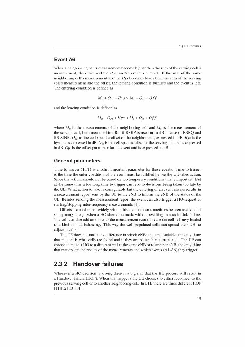
5.5 Simulation 5 - Worst case gradientThe outcome from implementing worst case gradient was successful and was done as

described in Section 4.5. The difference in throughput between the different time intervals

were very small and the late A2 measurement reports did not seem to correlate to HOF

even though they have decreased a lot compared to previous simulations. Inter-frequency

on the other hand has been increased for this simulation, as seen in Figure 5.24. The

HOFs from the simulation were compared with the HOFs from simulation 4 - Gradients

combined, for the different UE speeds and can be seen in the Figures 5.25, 5.26, 5.27 and

5.28.


frequency for the UEs are shown with different time intervals. The

first value in the legend refers to the short gradient interval and the

second value refers to the long gradient interval. All intervals are

not shown in the figure, but all interval settings follow the same

pattern: short interval at 0.04 s are all gathered in the highest line

bundle and at 0.25 s are all gathered in the lower line bundle.

54

5.5 Simulation 5 - Worst case gradient

UE speed 3 km/h

Figure 5.25: HOFs from simulation 4 (combined) and 5 (worst

case) are shown for the different time intervals with their own cor-

responding axis, 4 above and 5 below.

UE speed 30 km/h




55

5. Results

UE speed 120 km/h




UE speed 350 km/h




56

Chapter 6Analysis

In this chapter the analysis of each individual simulation is made based on the results

from the corresponding simulation presented in Chapter 5. When it has been possible the

analysis have been made on the simulation as a whole, without considering the UE speed,

else the analysis has been divided into the different speeds.

6.1 Simulation 1 - Environment evaluationThe results from the simulations with case 1 indicate that the reception was too good in

the cell deployment for inter-frequency measurements to make any difference to the result.

Based on this conclusion there is no further interest in investigating case 1.

Case 3 on the other hand showed great improvement in number of HOFs and through-

put with A1, A2 and A5 turned on, as can be seen in Figure 5.1 and Figure 5.2. This

means that the inter-frequency measurements and HOs have an impact on the result and

the environment can be used for investigating inter-frequency HO’s relation to the UEs

performance.

6.2 Simulation 2 - Negative gradientAs seen in Figure 5.3 the throughput did not change much between the different intervals

even if there were some improvements on both time spent measuring inter-frequency and

number of HOFs. It seems that inter-frequency measurements and HOFs did not influence

the throughput enough to make a noticeable difference in the results.

The time spent measuring inter-frequency was greatly reduced in some cases when

using the algorithm which can be seen in Figure 5.4. More specifically the time spent were

reduced more when a larger time interval were used in the algorithm. Another pattern that

appeared with greater time intervals used in the algorithm was the increase of late A2

57

6. Analysis

measurement reports as seen in Figure 5.5, 5.6, 5.7 and 5.8. One possible reason for this

is that large time intervals react slower to sudden changes in RSRP and therefore the A2

event triggers later and thus there is a bigger risk for late A2 measurement reports.

When looking into how the inter-frequency measurements changed within one interval

(the case of 0.04 s shown in the figures) there seem to be a larger risk that the amount of

measurements is increased when looking at the higher UE speeds. In Figure 5.12 (UE

speed 350 km/h) there is a 70 % risk that the amount of inter-frequency measurements

increase. In the case with UE speed 3 km/h (Figure 5.9) there is a 75 % chance of improv-

ing the results. In between these results the UEs with speed 30 km/h (Figure 5.10) have a

70 % chance of improving the measurements and the results from 120 km/h (Figure 5.11)

provide a 50 % probability.

6.2.1 UE speed 3 km/hWhen looking at the slow moving UEs (3 km/h) in Figure 5.5, there seems to be no rela-

tion between the number of late A2 measurement reports and the number of HOFs. The

simulations with a gradient interval of 1.0 s and 1.75 s had the lowest number of HOFs

and the later had the lowest amount of inter-frequency measurements.

As previously mentioned the chance of improving the amount of inter-frequency mea-

surements in the 0.04 s interval are 75 %. The probability to improve the result by at least

2.5 s is 47.5 %, making the probability of a very small improvement (between 0 s and

2.5 s) 27.5 % of the total outcome. When looking at the negative results there are a 2.5 %

risk the outcome would be 2.5 s worse or more than before. As a total it would seem a

rather small risk and pretty much to gain from using this gradient interval at this speed of

a UE.

6.2.2 UE speed 30 km/hThe best results was achieved with 0.5 s gradient interval. It had the lowest number of

HOFs and a lower amount of inter-frequency than the baseline simulation. There were

other intervals that had a lower amount of inter-frequency measurements but there were

significantly more HOFs in them. The A2 measurement reports were consistently a bit

late but this seemed to have no noticeable impact on the overall result, see Figure 5.6.

As stated earlier, the chance of improving the inter-frequency measurements in the

0.04 s interval are 70 % based on the run simulations. The probability of making it at least

2.5 s better are 40 % and the probability of making it at least 2.5 s worse for the UEs are

6 %. Once again the risk is pretty low, even though it has increased a little bit, there is still

much to gain from using this gradient interval at this speed of a UE.

6.2.3 UE speed 120 km/hA gradient interval of 0.04 s was the best at this UE speed with 387 HOFs compared to

426 HOFs when looking at the baseline, see Figure 5.7. When using a gradient interval of

1.0 s a result with almost as few HOFs as when using 0.04 s was achieved but also with a

decrease of 1 s for average time spent measuring inter-frequency.

58


At this speed it could be reasoned that a connection between late A2 measurement

reports and HOFs could be seen. As seen in Figure 5.7 the number of late A2measurement

reports seems to follow the number of HOF over the different time intervals.

The probability of an improvement of the inter-frequency measurements in the 0.04 s

interval are, as previously stated, 50 %. There is a 35 % probability of getting an improve-

ment of 2.5 s or more and a 12.5 % risk of getting a 2.5 s deterioration or worse. As seen

there is a bigger chance of getting a large improvement than a large deterioration in this

speed but there is still a fifty-fifty chance if there will be an improvement at all.

6.2.4 UE speed 350 km/h

As seen in Figure 5.8, the result from the baseline simulation was the best when consider-

ing the number of HOFs. At the same time, the number of late A2 measurement reports

was pretty high. Later when using the gradient algorithm, there seem to be a high number

of HOFs when there was a low number of late A2measurement reports. This could be con-

cluded to there being no connection between late A2 reports and HOFs when considering

this UE speed.

One thing that stood out in Figure 5.4 were that the baseline simulation had lower

time in inter-frequency than the simulations using the algorithm with the intervals 0.04 s,

0.25 s and 0.5 s on UEs with the speed of 350 km/h. One possible reason for this is that

for UEs with higher speeds there were more situations when the RSRP dropped very fast

and small time intervals react faster to this. Resulting in inter-frequency measurements

getting turned on earlier than when the algorithm is not used.

As mentioned there is a 70 % risk of increasing the amount of inter-frequency mea-

surements when looking at the 0.04 s interval and a 42.5 % risk of getting a result that is

2.5 s worse or more. The chance of improving the result with 2.5 s or more is 15 % so the

stakes for improving the amount of measurements at this speed are pretty high.

6.3 Simulation 3 - Positive gradientAs seen in Figure 5.13 there was small variations in the result overall when trying the

different time intervals. However the simulation without the gradient had the highest time

spent measuring inter-frequency on all UE speeds. When one or both of the time intervals

were increased the time spent measuring inter-frequency was slightly lowered but at the

cost of a slight increase of HOF, as seen in Figure 5.14.

Depending on what to prioritize there are two different approaches to take, either go

with the lowest time spent measuring inter-frequency or the lowest amount of HOF. It was

reasoned that the low gain in inter-frequency was not worth the increase in HOF, therefore

the interval setting 0.04 s with 0.5 s to trigger A1 were considered the best and used for

the coming simulations.

59

6. Analysis

6.4 Simulation 4 - Gradients combinedThe time spent measuring inter-frequency was lower than without the algorithm as seen

in Figure 5.15, especially for the UE speeds 120 and 350 km/h and the higher intervals.

When looking at Figure 5.20, UEs with speed 3 km/h, there seem to be no noticeable

change in the probability for a deterioration compared to only using the negative gradient.

The results for the improved UEs on the other hand show a slight improvement, providing

a bit greater values given a certain probability.

In Figure 5.21 the UEs had the speed 30 km/h. The results in the figure shows a slight

improved (lower) probability for the impaired UEs compared to the negative gradient sim-

ulation. The improved UEs show larger values than the negative gradient simulation.

As seen in Figure 5.22 with UE speed 120 km/h, the probability for a deterioration is

lower than the negative gradient simulation and the deteriorations are also smaller. There

is also a higher chance of changing to the better rather than to the worse compared to

without the algorithm, in contrast with the negative gradient simulation where there is a

greater probability the UE’s inter-frequency measurements change to the worse.

The overall result is better in this simulation with UE speed 350 km/h (Figure 5.23)

compared to both the baseline simulation and with the algorithm using the negative gra-

dient. There is still a risk that there is deterioration for an individual UE compared to not

using the algorithm. However, the probability of improving the result for the individual

UEs is greater than the risk of making it worse. The probability of deterioration is lower

than with the negative gradient and if there is deterioration, the deterioration is lower.

The HOFs compared to simulation 2 - Negative gradient varied in terms of improve-

ment and deterioration. For UE speeds 30 km/h and 120 km/h the HOFs overall had

decreased (Figure 5.17 and Figure 5.18) but for UE speeds 3 km/h and 350 km/h the re-

sults varied between the different time interval settings (Figure 5.16 and Figure 5.19). The

reason for the increase in HOF (for some settings) could probably be explained by the

risk of turning off inter-frequency measurements when they were needed (by the positive

gradient). Overall the HOF was lowered or approximately the same but accompanied by

a decreased time spent measuring inter-frequency, which is very positive.

6.5 Simulation 5 - Worst case gradientThe purpose of this simulation was to decrease the HOF as much as possible and it was

successful for the UE speeds 3 km/h and 350 km/h, as seen in Figure 5.25 and Figure 5.28.

Most noticeable was the results from 350 km/h because of the fact that this was the first

time the number of HOFs were lower than the baseline simulation, with a decrease of

25HOFs. But at a high cost in time spentmeasuring inter-frequency, from 7.25 s to 15.42 s,

an increase of 113 %. The results from UEs with speed 3 km/h also showed the lowest

number of HOFs compared to all simulations, 128 HOFs compared to the 137 HOFs that

the simulation 2 - Negative gradient achieved. In conclusion there is a high cost in time

spent measuring inter-frequency, which is consistent through all interval settings and UE

speeds (see Figure 5.24). It all comes down to howmuch increase in time spent measuring

inter-frequency a HOF is worth.

60

6.6 Summary

6.6 SummaryTo sum up, no setup was found that gave the lowest time spent measuring inter-frequency

and the lowest amount of HOF for all UE speeds. This means depending on what to pri-

oritize different gradient algorithm settings could be used. Some of the simulation results

stood out from the others and these can be seen in Table 6.1. First in the table is the base-

line simulation for comparison, second comes the simulation with the lowest time spent

measuring inter-frequency, third to seventh had the lowest HOFs for the corresponding

UE speeds and total, lastly is the simulation that gave a balanced result with low inter-

frequency and a fairly low amount of HOFs.

Table 6.1: A summary of the simulation results of interest. The

values represent the difference between the corresponding simu-

lation and the baseline simulation.

Simulation Quality factor 3 km/h 30 km/h 120 km/h 350 km/h TotalBaseline HOF 150 299 426 402 1277

Inter-frequency [s] 14.70 10.72 8.29 7.25 10.24

Combined HOF -3 -3 -36 +28 -14

2.00 s Inter-frequency [s] -5.57 -4.22 -3.92 -3.66 -4.34

Worst case HOF -22 +21 -42 +42 -1

0.25 s & 1.00 s Inter-frequency [s] +8.95 +8.47 +5.94 +5.12 +7.12

Negative HOF +3 -10 -27 +11 -23

0.50 s Inter-frequency [s] -4.10 -2.33 -0.22 +0.38 -1.57

Worst case HOF -15 +31 -51 -6 -41


Worst case HOF -12 +11 -39 -25 -65


Worst case HOF -21 +10 -43 -24 -78

0.04 s & 0.75 s Inter-frequency [s] +10.24 +10.52 +8.13 +6,95 +8,96

Combined HOF -11 0 -37 +15 -33

1.75 s Inter-frequency [s] -5.39 -3.99 -3.72 -3.49 -4.14

61

6. Analysis

62

Chapter 7Discussion

In the discussion the validity of the report’s different parts as well as the report as a whole

is discussed. The discussion explains how the experiments have been carried out and if

they could have been carried out differently. The given results are discussed and if any

part of the result is missing or could be presented in another way. Finally the analysis of

the different experiments and an analysis of the overall result are discussed.

7.1 The environmentAll the simulations were executed with either 3GPP case 1 or case 3 as cell deployments.

This has influenced the results in many ways. The simulated cell deployments are not re-

alistic in the sense of the even distribution of the eNBs, that there are no radio interference

except for the UEs themselves and that there is no radio shadow. But because this work was

a study and exploration of a new concept, some simplified arrangements were necessary

to isolate the algorithm’s influence on the UEs and the overall result. It was also important

that the cell deployment created an environment where inter-frequency measurements had

an important role and were common so it could be properly studied and gave an impact to

the result. Case 3 was concluded to do this with the chosen simulation settings.

The UEs themselves and their behavior in the simulations are also questionable. All

UEs moved in straight lines with constant specific speeds which could be reasoned is fairly

unrealistic. But as already mentioned, some simplified arrangements were necessary to

isolate the intended situation so it could be studied. The same goes with the number of UEs

which was set to 30 for all the simulations, where possible UE interference was avoided

by keeping the quantity low. Throughout all simulations the UEs’ speeds influenced the

result a lot and it could be reasoned that different speeds should be tested. The reason for

choosing these speeds from the beginning was mainly based on 3GPP’s recommendations

when testing mobility, but for a more reassuring result more speeds could be tested. When

the simulation started the UEs were automatically connected to the cells with the short

63

7. Discussion

range frequency because it created a scenario where UEs would benefit from making an

inter-frequency HO. That setting was important so inter-frequency HOs made a larger

impact on the result, but it also meant the algorithm has been primarily tested on scenarios

where the inter-frequency HOs gives the best result which makes the result a little biased.

The simulator itself has also made a large impact on the results. The software envi-

ronment that was used is very complex and might contain some minor unknown faults or

errors, as most software does. How close to the reality the simulator was is out of this

thesis scope, but should be kept in mind when looking at the results.

7.2 The resultsIn the results and analysis it has been concluded that the throughput have not been affected

or have been affected so little that it is not visible in the result. When the results from the

second simulation (Simulation 2 - Negative gradient) showed that the throughput was not

affected in any noticeable way, the procedure of how the average throughput was calculated

was reviewed to verify the correctness of the calculation. The calculation seemed right and

no correction was made to the way of calculating the average throughput. Through the rest

of the simulations (3-5) no significant difference in throughput was found.

One explanation to the unaffected throughput could be due to the fact that there are very

fewUEs compared to the number of available cells. The UEs and eNBsmight have had the

possibility to make a rescheduling of the data transmissions and in that way eliminate the

difference that would occur due to a connection loss or any other event that might affect the

throughput. There might also be some other factors that have not been found or not been

taken under consideration in this work that could influence the behavior of the throughput.

In contrast to the throughput, the time spent measuring inter-frequency was success-

fully controlled and decreased throughout the simulations. The negative gradient worked

best at the lower speeds 3 km/h and 30 km/h while the positive gradient functioned best at

the higher speeds 120 km/h and 350 km/h. Overall in the gradient combined simulation

the inter-frequency measurements in the lower speeds were reduced with more seconds

compared to the baseline simulation.

The longer the intervals, the less time spent measuring inter-frequency, but this comes

with a cost of increased HOF (in most cases). As time spent measuring inter-frequency

gets improved (lower) the risk of increasing the time spent measuring is lowered as well,

especially for the low UE speeds where the risk is very small. The gradient combined

algorithm did not introduce a high risk and high reward, the chance to lower the time

spent measuring inter-frequency is always greater than the risk of introducing more inter-

frequency measurements, which is very positive.

It is safe to say that the number of HOFs have differed between the simulations and

within them. It has been harder to say if the changes made in the settings have affected

the HOFs and to what degree. When looking at the different figures showing HOF most

of them tend to mimic a zigzag like pattern.

On a conceptual level there is three types of HOFs; those HOFs that are hard to avoid,

those HOFs that seems to have no correlation to the algorithm at all and those HOF that

could be avoided by introducing the algorithm. It is hard to know the distribution of these

three types of HOFs which makes the evaluation of the HOFs difficult. To get more in-

64

7.3 Other aspects

sights about this the worst case scenario simulation was created, where inter-frequency

measurements were introduced with the hope of reducing the HOFs. The HOFs in the

simulation were in some cases reduced and in some cases unaltered, which leaves the

authors wondering about the HOFs correlation to the introduced algorithm.

One important aspect of this work has been the value of a HOF. It could be reasoned

that there is an active transmission and a HOF occurs due to too few inter-frequency mea-

surements (in some cases). If the throughput in total would still be higher than the total

throughput when making enough inter-frequency measurements to avoid the HOF, result-

ing in the same amount of data transmitted in both cases. Then there might be some jus-

tification for not doing all those measurements. The comparison would need to be looked

upon with all the consequences that come with a HOF, such as retransmitting data and

finding a new HO candidate.

When starting this work, we had a hypothesis that there would be a correlation between

the number of HOFs and the number of late A2 measurement reports. But as seen in the

results from the different simulations there seem to be no such correlation. Those few oc-

casions when there seem to be some kind of connection between the late A2 measurement

reports and the number of HOFs might as well be a coincidence. There might be some

possible explanations to this. One example could be the fact that UEs is not as sensitive

to the RSRP being too low as initially thought. This means there are other unidentified

factors that influence the numbers of HOF more than the introduction of the gradient al-

gorithm. Another possible reason is if the threshold would be too high, resulting in a late

A2 measurement report that is in fact not too late, even thought it was recorded as one.

Another factor that could be discussed is the time used to decide whether or not the A2

measurement report would be too late. The time chosen might as well be to short or too

long, resulting in faulty recordings.

When deciding on which settings that is the best it comes down to two important fac-

tors to have in mind: What UE speeds to prioritize and what is more important between

inter-frequency measurements and HOFs. If the goal is to have a setting that gives the

overall best results for the different UE speeds, there is a worst case gradient simulation

(0.04 s & 0.75 s) that gives the lowest number of HOF combined for all speeds. But on the

other hand it gives an increase in time spent measuring inter-frequency compared to many

other settings. If the goal is to lower the time spent measuring inter-frequency instead, the

best is the gradient combined 2 s settings, which have more HOF compared to previously

mentioned worst case gradient setting. To decide on what gradient algorithm settings to

use is not easy, and becomes even more complex if weighted UE speeds gets involved.

7.3 Other aspectsThe time spent measuring inter-frequency has been decreased with the help of the gradi-

ent algorithm but at the same time some extra calculations has been introduced which are

more complex than using static thresholds. The simulator did not offer any possibility to

measure the power consumption for the kind of calculations the algorithm introduced. But

in perspective to other calculations made by the UE, e.g., screen rendering or signal mod-

ulation, the introduced extra calculations are very few in comparison. The inter-frequency

measurements themselves also consume extra power which is avoided when using the gra-

65

7. Discussion

dient algorithm. So in practice, the inter-frequency measurements have been reduced at

the cost of almost nothing in power consumption. On the other hand, the algorithm might

introduce a need for some extra processing cycles, which might influence the processor’s

capability in a negative way.

When looking at the possibility to implement this in the current setting with eNB and

UE there is a great challenge in convincing the 3GPP organization to accept this change in

the standard. There would need to be further investigation within the area to make sure the

improvements are worth more than the effort needed to implement this algorithm. There

might also be a conflict in what exact algorithm to use, there are many possible ways to

modify the algorithm.

The configuration settings sent from the eNB to the UEmight also need to be expanded

to be able to send settings such as more thresholds and intervals. The UE in turn needs to

be able to receive these settings and adapt to them. This means that each of the different

manufacturers needs to implement the algorithm in their UEs. The UEs needs to adapt

both in terms of being able to receive the settings and in terms of storing extra variables in

the memory and handling them. There might also be a need to keep the old way of doing

it, meaning there might be a setting where the eNBs need to be able to send different kind

of settings depending on if the UE uses the algorithm or not.

In theory, the concept of the algorithm could also be implemented in other devices,

such as eNBs or some other access technologies. This could mean that 3GPP would not

need to get involved when introducing a change. The same goes for the measurement unit

(RSRP) as this work has focused on, the concept could be used to other units, i.e. RSRQ.

66

Chapter 8Conclusions

In this work experiments have been made where the change in signal quality has been used

to try to determine when a HO should be made. This has been done by implementing an

algorithm that saves old measurements and calculates the gradient of the change in the

signal quality. The algorithm has been used both to determine when inter-frequency mea-

surements should be turned on and off. The results show that the algorithm is inconsistent,

but there are results that show improvements compared to the baseline simulation. The in-

consistency is hard to explain but might occur due to some environment settings who have

not been looked upon or some unknown factor of the algorithm. The improvements were

in terms of reducing the amount of inter-frequency measurements while keeping the num-

ber of HOFs low. The UE downlink throughput was unaltered throughout the experiments

and the late A2 measurement reports showed no correlation to the variations in the results.

Is it possible for the UE in the simulator to find the current signal quality’s rate ofchange, based on its measurements?

It was concluded early on in simulation 2 - Negative gradient, that it is possible to find

the signal quality’s rate of change. This was done by saving old measurements and their

time and calculating the gradient from these values. The signal power was quantified by

using RSRP but any signal power/quality indicator in theory would be applicable to this

work, as long as it changes over time.

Based on the rate of change, is it possible to predict when a handover (HO) shouldbe made (both initiated and finished)?Yes, it was concluded that it is possible to predict when a HO should be both initiated

and finished based on the calculations of the signal quality’s rate of change. However, the

prediction was not 100 % accurate. There was very fast changes in RSRP which could

not be predicted and there was some other situations where HOs was needed, that was

unrelated to RSRP measurements, which also could not be predicted.

67

8. Conclusions

Will this new way be more efficient than current solution, in terms of calculation ef-fort and measurement effort without compromising the Quality of Service (QoS)?

The new algorithm is more efficient in terms of calculation effort. Some few extra

calculations have been introduced in conjunction with the new algorithm. But the im-

provement (lowering) of the amount of measurements in terms of inter-frequency has been

reasoned to be far more important than the few extra calculations the algorithm have in-

troduced.

By optimizing, the time spent measuring inter-frequency was successfully lowered.

With the help of the predictions of when the HO should be made, the start of inter-

frequency measurements could be delayed to when they were needed or turned off if they

were not needed at all. In this way the measurement effort could be made more efficient

than the current solution.

In terms of QoS, more specifically throughput and HOFs, the results are more uneven.

Throughout the simulations the throughput was more or less unchanged even if the time

spent measuring inter-frequency and HOFs was reduced. The probable reason behind this

is the fact that there are very few UEs compared to the available cells in the simulations.

The UEs and the eNBs then had the possibility to reschedule the data transmissions and

in that way eliminate any throughput differences. The HOFs were in some simulations

reduced and in some simulations increased. The HOFs varied a lot based on what speed

the UE had and how the gradient algorithm was used. No settings was found for reducing

the HOFs through all the UE speeds and in some simulations the HOFs seemed to have no

(or low) correlation to the time spent measuring inter-frequency, which not was expected.

The probable reason for this unexpected pattern is that the HOF is more dependent on

other factors than the time spent measuring inter-frequency, which has not been identified

by this work. For some algorithm settings the HOFs were greatly reduced but most often

with the cost of more time spent measuring inter-frequency. It all comes down to what to

prioritize, time spent measuring inter-frequency or HOFs and for which UE speeds.

68

Chapter 9Future Work

There are several different ways to continue from this work apart from looking into differ-

ent variants of how to find the ultimate way to minimize the inter-frequency measurements

while keeping HOFs low. There could be other ways to adapt the measurements to the

UE’s speed which works better than the suggested way in this report. It could also be an

idea to look into deploying this kind of algorithm on other platforms where calculations

are cheap and measurements expensive. Lastly it would be interesting to see if the intro-

duced changes with using the algorithm could be seen in the overall result from a more

reality-based simulation environment and in the end in the actual reality.

Since the average UE throughput was not unaffected, it would be interesting to have

more simulations made where this is researched. One aspect could be to maximize the load

of the cells so the scheduler would not have enough capacity to reschedule the throughput

for the UE.

Depending on how much calculation that could be introduced in the UE or the eNB

there are some alternative ways to implement the algorithm that might improve the result

even further. There could for example be weight added to the more recent measurements

or to the measurements with worse reception, giving them a greater impact if evaluating

more than one gradient.

If increased storage and calculation effort is not a problem the calculation could result

in a curve from three or more points based on the measurement values. Whether the

decision is to make a HO or turn off the inter-frequency measurements, this way more

information would be provided to base the decisions on.

If the introduced calculation effort is a problem it could investigated how seldom the

calculation of the gradient needs to be done without compromising the effects of the algo-

rithm. It could be reasoned that the calculations are not needed if the gradient is positive

for a period of time or if the RSRP is good enough.

If an optimized algorithm was found, it would be interesting to see if it is possible to

implement the algorithm on another platform, e.g., an eNB, successfully. The measure-

ments would need to be made in the eNB or be sent to it. From there the calculations could

69

9. Future Work

be made and a decision taken based on the result. If making the calculations in the eNB,

there seem to be no need to make any changes in the standards from 3GPP.

70

Bibliography

[1] C. Johnson. Long Term Evolution in bullets. Chris Johnson, Northampton, 2nd ed.,

version 1. edition, 2012.

[2] 3GPP. Evolved Universal Terrestrial Radio Access (E-UTRA); Base Station (BS)

radio transmission and reception. TS 36.104, 3rd Generation Partnership Project

(3GPP), 2015.

[3] 3GPP. Evolved Universal Terrestrial Radio Access (E-UTRA); Physical layer; Mea-

surements. TS 36.214, 3rd Generation Partnership Project (3GPP), 2015.

[4] M.B. Hcine and R. Bouallegue. Analytical downlink effective sinr evaluation in

lte networks. In Advanced Information Networking and Applications Workshops(WAINA), 2015 IEEE 29th International Conference on, pages 376–381, March

2015.

[5] 3GPP. Evolved Universal Terrestrial Radio Access (E-UTRA) and Evolved Universal

Terrestrial Radio Access Network (E-UTRAN); Overall description; Stage 2. TS

36.300, 3rd Generation Partnership Project (3GPP), 2015.

[6] M. Rumney. LTE and the evolution to 4G wireless: design and measurement chal-lenges. Agilent Technlogies Publication, [Santa Clara, CA], 2009.

[7] 3GPP. Evolved Universal Terrestrial Radio Access (E-UTRA); Radio Resource Con-

trol (RRC); Protocol specification. TS 36.331, 3rd Generation Partnership Project

(3GPP), 2016.

[8] 3GPP. Vocabulary for 3GPP Specifications. TR 21.905, 3rd Generation Partnership

Project (3GPP), 2015.

[9] N. Hassan, K. Elkhazeen, K. Raahemiafar, and X. Fernando. Optimization of control

parameters using averaging of handover indicator and received power for minimizing

ping-pong handover in lte. In Electrical and Computer Engineering (CCECE), 2015IEEE 28th Canadian Conference on, pages 92–97, May 2015.

71

BIBLIOGRAPHY

[10] M.S.I. Khan, M.M. Rahman, K. Raahemifar, J. Misic, and V.B. Misic. Self-

optimizing control parameters for minimizing ping-pong handover in long term evo-

lution (lte). In Communications (QBSC), 2014 27th Biennial Symposium on, pages118–122, June 2014.

[11] 3GPP. Telecommunication management; Self-Organizing Networks (SON) Policy

Network Resource Model (NRM) Integration Reference Point (IRP); Requirements.

TS 32.521, 3rd Generation Partnership Project (3GPP), 2012.

[12] B.K.S. Fatty and Po-Chiang L. Mobility robustness optimization in wireless mobile

networks. In Ubiquitous and Future Networks (ICUFN), 2015 Seventh InternationalConference on, pages 624–629, July 2015.

[13] I.N.M. Isa, M.D. Baba, R. Ab Rahman, and A.L. Yusof. Self-organizing network

based handover mechanism for lte networks. In Computer, Communications, andControl Technology (I4CT), 2015 International Conference on, pages 11–15, April2015.

[14] I.N.M. Isa, M.D. Baba, A.L. Yusof, and R. Ab Rahman. Handover parameter opti-

mization for self-organizing lte networks. In Computer Applications Industrial Elec-tronics (ISCAIE), 2015 IEEE Symposium on, pages 1–6, April 2015.

[15] 3GPP. Evolved Universal Terrestrial Radio Access (E-UTRA); Further advance-

ments for E-UTRA physical layer aspects. TR 36.814, 3rd Generation Partnership

Project (3GPP), 2010.

[16] 3GPP. Physical layer aspect for evolved Universal Terrestrial Radio Access (UTRA).

TR 25.814, 3rd Generation Partnership Project (3GPP), 2006.

72

Institutionen for Elektro- och informationsteknik | Lunds Tekniska HogskolaRedovisas 3 Juni 2016

Examensarbete: Optimering av algoritmer for mobilitiet i cellulara systemStudenter: Bernt Christensen, Olof KnapeHandledare: Fredrik Tufvesson (LTH), Niklas Holmqvist (Ericsson), Jan Wichert (Ericsson)Examinator: Fredrik Rusek

Optimering av matningar i mobilnatetPOPULARVETENSKAPLIG SAMMANFATTNING AV Bernt Christensen, Olof Knape

DET GORS HELA TIDEN MATNINGAR MOT MASTER I MOBILNATET FRAN DIN MOBIL, FOR ATT SE TILL ATT DU HARBASTA MOJLIGA MOTTAGNING. VART ARBETE VISAR ATT DET GAR ATT MINSKA MANGDEN AV DESSA MATNINGARMED 40 % SA ATT MER RESURSER KAN ANVANDAS TILL ATT SKICKA DATA.

Antalet enheter som kopplas upp till det mobilanatet okar standigt samtidigt som anvandarna har hogaforvantningar pa tillganglighet och staller allt hogre kravpa hog overforingshastighet. Bland annat ska det okandeanvandandet av olika streaming-tjanster tillfredsstallas.Det ar darfor valdigt viktigt att natverket kan tillhan-dahalla detta. Samtidigt finns det begransningar for hurmanga mobila enheter som kan vara uppkopplade sam-tidigt mot en mobilmast. Mobilmasten har ocksa en be-gransning i hur mycket data den kan hantera. Darfor ardet viktigt att de mobila enheterna ar jamnt fordeladebland de tillgangliga mobilmasterna. Det vill saga det arviktigt att belastningen mellan mobilmasterna utjamnasi sa stor utstrackning som mojligt. Detta kanske latersom en latt uppgift, men med tanke pa att de mobilaenheterna ror sig i olika monster och hastigheter hela ti-den blir det mycket svarare, forutsattningarna forandrasstandigt. For att de mobila enheterna ska kunna varauppkopplade mot ratt mast, med basta mojliga mot-tagning, gors matningar av signalstyrkan mot de oli-ka mobilmasterna i omgivningen. Dessa matningar arnodvandiga men de som gors mot andra frekvenser anden som anvands ar ocksa valdigt resurskravande. Pre-cis som en vanlig gammaldags radioapparat hemma kanman inte lyssna pa en radiokanal samtidigt som man le-tar efter nya radiokanaler (frekvenser). Pa samma sattkan inte den mobila enheten lyssna pa andra frekvensermed battre mottagning samtidigt som den tar emot da-ta pa den ursprungliga frekvensen. Darfor ar det viktigtatt dessa matningar mot andra frekvenser halls pa ettminimum och det ar dar vart arbete kommer in.

Vi har alltsa forsokt att minska tiden som behovs foratt leta efter nya mobilmaster och pa sa satt oka tidenenheten kan skicka och ta emot data. Iden bakom varalgoritm gar ut pa att studera hur snabbt signalstyr-kan mot den nuvarande masten forandras. Pa sa satt far

vi mer information om ett eventuellt mastbyte behovergoras och nar, vilket inte den traditionella metoden kan.Forhoppningen var att detta skulle fungera oberoende avhur snabbt den mobila enheten ror sig. Detta jamfordesmot den traditionella metoden i en simulator fran Er-icsson. Resultatet var positivt och vi lyckades minska deresurskravande matningarna i genomsnitt med ca 40 %samtidigt som antalet tappade uppkopplingar minskademed ca 3 %. Tyvarr var algoritmen inte helt oberoendeav hur snabbt den mobila enheten rorde sig, de hogstahastigheterna var svara att parera. Det i ovrigt positi-va resultatet skapar anda incitament att undersoka omdet gar att minska antalet matningar annu mer. Det ha-de ocksa varit intressant att prova algoritmen i en riktiglabbmiljo. I vart arbete undersoktes enbart en 4G-miljo(LTE), men algoritmen skulle relativt latt kunna modi-fieras till att passa andra mobila plattformar och tekno-logier.

En mobiltelefon ror sig mellan tva mobilmaster,mobiltelefonen gor darfor ett mobilmastbyte foratt vara uppkopplad mot den mobilmast med bastmottagning.

Op

timizatio

n o

f Alg

orith

ms fo

r Mo

bility in

Cellu

lar Systems

Department of Electrical and Information Technology, Faculty of Engineering, LTH, Lund University, 2016.

Optimization of Algorithms forMobility in Cellular Systems

Bernt ChristensenOlof Knape

Series of Master’s thesesDepartment of Electrical and Information Technology

LU/LTH-EIT 2016-509

http://www.eit.lth.se

Be

rnt C

hriste

nse

n &

Olo

f Kn

ap

e

Master’s Thesis

Documents

Optimization of Algorithms for Mobility in Cellular Systems