Embed Size (px)
Citation preview

KSII TRANSACTIONS ON INTERNET AND INFORMATION SYSTEMS VOL. 10, NO. 9, Sep. 2016 4044 Copyright ⓒ2016 KSII
Optimization of Energy Consumption in the Mobile Cloud Systems
Pan Su 1, Wang Shengping 1,2, Zhou Weiwei 1 and Liu Shengmei 1
1Key Lab of “Broadband Wireless Communication and Sensor Network Technology”(Nanjing University of Posts & Telecommunications), Ministry of Education
Nanjing 210003, China [e-mail: [email protected]]
2Jiangsu Power Design Institute Co., Ltd. of China Energy Engineering Group Nanjing, 211102, China
[e-mail: [email protected]] *Corresponding author: Pan Su
Received February 14, 2015; revised May 14, 2015; revised May 27, 2016; accepted July 27, 2016;
published September 30, 2016
Abstract
We investigate the optimization of energy consumption in Mobile Cloud environment in this paper. In order to optimize the energy consumed by the CPUs in mobile devices, we put forward using the asymptotic time complexity (ATC) method to distinguish the computational complexities of the applications when they are executed in mobile devices. We propose a multi-scale scheme to quantize the channel gain and provide an improved dynamic transmission scheduling algorithm when offloading the applications to the cloud center, which has been proved to be helpful for reducing the mobile devices energy consumption. We give the energy estimation methods in both mobile execution model and cloud execution model. The numerical results suggest that energy consumed by the mobile devices can be remarkably saved with our proposed multi-scale scheme. Moreover, the results can be used as a guideline for the mobile devices to choose whether executing the application locally or offloading it to the cloud center. Keywords: Mobile cloud computing, energy efficiency, stochastic wireless channel, dynamic scheduling.
http://dx.doi.org/10.3837/tiis.2016.09.002 ISSN : 1976-7277

KSII TRANSACTIONS ON INTERNET AND INFORMATION SYSTEMS VOL. 10, NO. 9, September 2016 4045
1. Introduction
Mobile Cloud Computing (MCC) is a new concept of Cloud Computing (CC) with a mobility feature, and it can be a way to overcome the limitations of mobile devices, such as the low computational power and insufficient memory capabilities. With the booming development of mobile communication, various functional applications can be easily downloaded from the application venders. At the same time, mobile devices can offload some applications over wireless networks to the cloud center for execution, which greatly reduces the requirements for storage and computing in mobile devices.
However, in recent years, the battery capacity is limited and is growing only 5% annually. In comparison to the booming mobile applications, the short battery life has become the bottleneck of the smart mobile devices [1]-[9]. As a result, special attentions have been devoted to decreasing energy consumption of mobile devices under the mobile cloud computing scenarios.
Kumar presented an energy consumption model to analyze whether or not the mobile device will offload applications to the cloud by comparing the computation energy in the mobile device with the communication energy for offloading applications to the cloud center [7], which is illustrated in Fig. 1. In general, the energy consumption of mobile devices could be optimized in two aspects. In the mobile execution model (ME model), the dynamic operating technique can be used to save the energy, i.e. the CPUs in the mobile devices dynamically adjust their operating parameters, such as the clock frequency, the supply voltage, etc. according to the computing power required by the applications. In the cloud execution model (CE model), the energy cost is mainly determined by the transmission rate and the channel states [8]. Normally, higher transmission bit rate in each time slot results in larger transmission power consumption in the time slot but less transmission time given the certain data size. On the contrary, lower transmission bit rate leads to less transmission power but more transmission time. So the minimized total energy consumed in the whole transmission time should be the result of carefully choosing (scheduling) of the transmission bit rate in each time slot. Meanwhile, the transmission bit rate in each time slot is relevant to the channel state. The optimal data transmission scheduling scheme will be the one that the transmission bit rate increases when the channel state is good and decreases when the channel state is bad. However, the researches in [7] [8] mentioned above mostly consider a fixed CPU operating scheme, i.e. CPU running with fixed parameters for a mobile application, and a fixed transmission bit rate scheme for the stochastic wireless channel in the cloud execution model.
Zhang revised the energy consumption models for both mobile execution and cloud execution by adopting a transmission data scheduling scheme in CE model and a dynamical computing model in ME model [9]. However, the ME model in [9] does not observe the difference of the computational complexity among various applications, which essentially affects the energy consumption while more complex applications usually consume more energy by CPUs in the mobile devices. As for the CE model in [9], due to the analyzing model used is rather simple, the channel gain was simply quantized into two states: “good” and “bad”. We will prove that it will cost unnecessary additional energy when channel gain under the middle level is directly quantized to the “bad”.
The above observations motivated our researches. The contributions of this paper lie in two aspects. First, we employ the asymptotic time complexity (ATC) to distinguish the
4046 Pan et al: Optimization of Energy Consumption in the Mobile Cloud Systems
applications’ computation requirements in the ME model to optimize the energy consumed by CPUs in mobile devices. Second, we adopt a multi-scale scheme to quantize the channel gain instead of dual scale scheme used in [9]. Based on this quantization scheme, we propose a new data scheduling method to reduce the energy consumption in the CE model and improve the accuracy of energy estimation. We will also prove that although the multi-scale quantization scheme adds the complexity of the analyzing model, the optimal energy consumption can still be obtained in the closed-form expression and the computing load for the system will not increase.
The rest of the paper is organized as follows. In section 2, we give the application profile model, the mobile execution energy model and the cloud execution energy model respectively. In section 3, we propose a new data scheduling scheme in the CE model and provide the closed-form solutions for the optimal energy consumption of two models. Section 4 discusses the numerical results and presents a guideline for the mobile devices to choose executing the application locally or offloading it to the cloud center.
Fig. 1. Mobile application executed in two modes: the mobile execution and cloud execution.
2. System Model In this section, we present the energy model with a modified application profile for the
applications executed on the mobile devices. Then, we give the transmission energy model with a multi-state quantized channel.
2.1 Mobile Application Profile Many details have influence on energy consumption of a mobile application, and here are
two aspects that should be taken into consideration [9]: • Input data size L: The number of data bits as the input for the application; • Application completion deadline T: The delay deadline before which the application
should be completed. Normally, energy consumption is proportional to the input data size and inversely
proportional to the completion deadline of the application. However, the distinction among different applications on energy cost cannot be ignored.
Numerical calculation applications can be accomplished with relatively fewer instructions,
KSII TRANSACTIONS ON INTERNET AND INFORMATION SYSTEMS VOL. 10, NO. 9, September 2016 4047
without occupying too much resource of CPUs. Whereas, applications like image retrieval or voice recognition require more instructions to get results, even with the same size of input data, which thereby occupy more resource of CPUs and cost more energy.
Since the CPU resource occupied by a mobile application is hard to calculate precisely, the asymptotic time complexity (ATC) is employed to distinguish different applications in energy cost. ATC is described by the function O(r(m)), where m is the size of the input data, e.g., the length of a voice section to be recognized, and r(m) is a function of m representing the running time. ATC is the upper bound for an algorithm’s running time when the input size goes to infinity with O (·) as the special notation indicating the upper bound [10]. ATC is usually expressed by one of the following equations according to the complexity of the applications: 1, log(𝑚),𝑚,𝑚 × 𝑙𝑜𝑔(𝑚),𝑚𝑎,𝑎𝑚 , etc.[10] For example, ATC of the voice recognition application is 𝑚2 in normal cases, where m is the length of the input voice [11].
As such, the modified application profile can be denoted as A(L, T, O(r(m))).
2.2 Mobile Execution Energy Model It is indicated that the CPUs tend to dominate the energy consumption of the mobile
devices [7]. When the application is executed on the mobile device, the energy consumed by the CPU is mainly determined by the workload [9], which is measured by the number of the CPU cycles required by the applications. Denoting the number of CPU cycles as W, then W is a random variable depending on the input data size and the complexity of the algorithm in the application. In CMOS circuits, the energy 𝜀𝜔 consumed in the ωth (ω≤W) CPU cycle is proportional to 𝑉2, where V is the supply voltage to the chip [12] [13]. Moreover, it has been observed that when operating at low voltage limits, the clock frequency of the chip, 𝑓, is approximately linear proportional to V [12]. Therefore, the energy consumed in the ωth CPU cycle can be expressed as,
𝜀𝜔(ƒ𝜔) = 𝑘 ∗ ƒ𝜔2 (1)
where k is the energy coefficient depending on the chip architecture [13]. The computation energy consumed in all W cycles is denoted as 𝜀𝑚 = ∑ 𝜀𝜔(ƒ𝜔)𝑊
𝜔=1 . In the ME model, the total energy consumption can be minimized by optimally
configuring the clock frequency of the chip via dynamic voltage scaling (DVS) method [14]. Note that a CPU can reduce its energy consumption substantially by running the application slowly. However, the application execution has to meet the delay deadline T, which suggests that the clock frequency cannot be constantly low. Hence, the clock frequency should be tuned to minimize the total energy consumption while meeting the application delay deadline. By this way, the minimum energy consumption in ME model is given by,
𝜀𝑚∗ = min 𝜳∈𝜱{𝜀𝑚(𝐿,𝑇,𝑂(𝑟(𝑚)),𝜳)} (2) where 𝜳 = {𝑓1,𝑓2 , … ,𝑓𝑊} is any clock-frequency vector that meets the delay deadline, 𝜱 is the set of all feasible clock-frequency vectors, and 𝜀𝑚(𝐿,𝑇,𝑂(𝑟(𝑚)) is the total energy consumption of mobile device.
Hence, the objective for minimizing the energy consumption is turned into finding out the fittest clock-frequency vector under the constrained time T. This optimization problem will be discussed in Section 3.
2.3 Cloud Execution Energy Model To simplify the cloud execution energy model, we make some assumptions as follows [8], [9]:
First, we assume that the binary executable file for the application has been replicated on

4048 Pan et al: Optimization of Energy Consumption in the Mobile Cloud Systems
the cloud center initially. Second, the display and network interface of the mobile device can be turned off when it is idle during the cloud execution. Hence, we only consider communication energy consumption of the cloud execution. Third, the receiving power is much lower than the transmission power. So we do not consider the scheduling of the output results from the cloud. Fourth, we assume that the channel between the mobile device and the cloud side is stochastic fading, and the current channel state information (CSI) is known to the transmitter. In addition, we don't consider any security issues on the cloud platform. Thus, the extra energy caused by operations concerning security, e.g., encryption and trust checking, is not taken into account.
As such, we only consider the optimal scheduling of input data transmission to achieve the minimum energy consumption on the mobile device. The optimization problem will be demonstrated in the following two sections.
2.3.1 Transmission Model Under the assumptions above, the energy consumed by mobile device in CE model is
mainly determined by the data transmission. Normally, the consumed energy is affected by the data size L and the delay deadline T in the application profile. The shorter the delay deadline or the larger the data size is, the more energy will be consumed for transmission. Besides, channel states, especially the path loss and multipath effect, also have an influence on the transmission energy. To simplify this model, we only consider the path loss, which is measured by the channel gain, in CE model. Since there is no closed-form expression between time delay and related transmission power in the wireless networks [15], approximating models should be built for practical system design.
In our designed model, the data transmission time is divided into T slots (from T to 1) and we adopt a monomial energy-bit function in [9] [16] and [17] to demonstrate the energy consumed per transmission time slot. Specifically, the energy consumed to transmit 𝑆𝑡 bits of data in the tth (t≤T) time slot is a convex monomial function, which denotes as,
𝜀𝑐(𝑆𝑡 ,𝑔(𝑡)) = 𝜆 𝑆𝑡𝑛
𝑔(𝑡) (3)
where n denotes the monomial order and 2 ≤n ≤5, depending on the modulation and encoding scheme. 𝜆 denotes the energy coefficient and 𝑔(𝑡) is the value of the channel gain at tth time slot. It is shown by [18] and [19] that the monomial function is fairly close to the power model indicated by Shannon’s formula if choosing an appropriate coefficient λ and order n. We present approximation method to obtain 𝜆 and n in the Appendix.
During the deadline T, the total energy consumed by the mobile device to transmit all L bits of data is ∑ 𝜀𝑐(𝑆𝑡 ,𝑔(𝑡))𝑇
𝑡=1 . It can be seen that the energy cost is mainly determined by the transmission rate and channel state. The minimized total energy consumption in the whole transmission time should be the result of carefully choosing the transmission bit rate in each time slot. We denote the optimal energy model for transmission as,
𝜀𝑐∗ = min𝑺𝒕���⃗ ∈𝜰��⃗ {𝜀𝑐(𝐿,𝑇), 𝑆𝑡���⃗ } (4) where 𝑺𝒕���⃗ = {𝑆1, 𝑆2 , … , 𝑆𝑇} is any data transmission scheduling that meets the data size requirement L, 𝜰��⃗ is the set of all feasible data scheduling vectors, and 𝜀𝑐(𝐿,𝑇) is the total energy consumption for a successful transmission by the mobile device.
Hence, the objective for minimizing the energy consumption in CE model is to find out the fittest data scheduling scheme meeting the data size and the delay deadline requirement. This optimization problem will be discussed in Section 4.
KSII TRANSACTIONS ON INTERNET AND INFORMATION SYSTEMS VOL. 10, NO. 9, September 2016 4049
2.3.2 Wireless Channel Model We only consider the slow fading in the wireless channel model. The Markov chain
model has been proved to be a successful mathematical tool to describe a stochastic wireless channel when the fading is slow [20]. The study in [21] suggests that a first-order Markov chain model is quite accurate and remains insensitive to different coding and modulation schemes. For this reason, the channel state was modeled as a first-order Markov chain in [9], where the channel gain was quantized into two states: “good” and “bad”. Although the dual-state Markov method helps to simplify the energy model, it causes the large quantization error and leads to unnecessary energy cost as well. It is demonstrated in [22] that multi-state Markov model works better in terms of capturing the statistics of deep shadowing and increasing the accuracy of estimating the channel performance. As a result, we adopt a multi-state Markov model as our wireless channel model, and we present some results of this channel model in Section 4.
The quantization of channel gain using a uniform quantizer with K states is denoted by, 𝑔�(𝑡) = arg min𝑔𝑘∈{𝑔1,𝑔2,…,𝑔𝐾}|𝑔(𝑡) − 𝑔𝑘| (5)
where the channel gain at time slot t is quantized to the one element of the set {𝑔1,𝑔2 , … ,𝑔𝐾} depending on its value. The set {𝑔1,𝑔2 , … ,𝑔𝐾} constitutes a Markov state space.
In the first-order Markov model, the current channel state is relevant to the last one. The probability of the channel gain from the ith state to the jth state is denoted as 𝑃𝑖𝑗, and the state transition probability matrix (TPM) P is,
𝑷 = �
𝑃11 𝑃12𝑃21 𝑃22
⋯ 𝑃1𝐾⋯ 𝑃2𝐾
⋮ ⋮𝑃𝐾1 𝑃𝐾2
𝑃𝑖𝑗 ⋮… 𝑃𝐾𝐾
� (6)
The stationary probabilities 𝑃(𝑗) of the channel gain at the state 𝑔𝑗 is the solution of the following linear system,
�𝑃(𝑗) = ∑(𝑃𝑖𝑗 ∗ 𝑃(𝑖))
∑𝑃(𝑗) = 1� (7)
3. Optimal Computation Energy in ME Model
In this section, we focus on the problem of minimizing the energy consumption in ME model. As demonstrated before, the objective is to set the clock frequency of chip properly to achieve the optimal computation energy consumption.
As is mentioned in section 2, the total computation energy 𝜀𝑚 = ∑ εω(ƒω)𝑊ω=1 is related
to the total number of CPU cycles required by the application W, which is a random variable with an empirical distribution [8] [9] [23], and generally proportional to the input data size and the complexity of the application. Hence, we map ATC complexity of the application into the virtual data size of the application. It follows,
𝑊 = 𝐺(𝐿) ∗ 𝑋 (8) where G(L) is the equivalent data size mapped from the ATC complexity and L is actual input data size of the application. G(L) takes the following expressions according to the complexity of the application, 1, 𝑙𝑜𝑔𝐿 , 𝐿, 𝐿 × log𝐿, 𝐿𝑎 ,𝑎𝐿 [24] [25] (e.g., for the voice recognition algorithm, G(L)= 𝐿2). X is a Gamma distributed random variable [23], and its probability distribution function (PDF) is given by,
p𝑥(𝑥) = 1𝛽∗𝛤(𝛼) �
𝑥𝛽�𝛼−1
𝑒−𝑥𝛽, for 𝑥 > 0 (9)
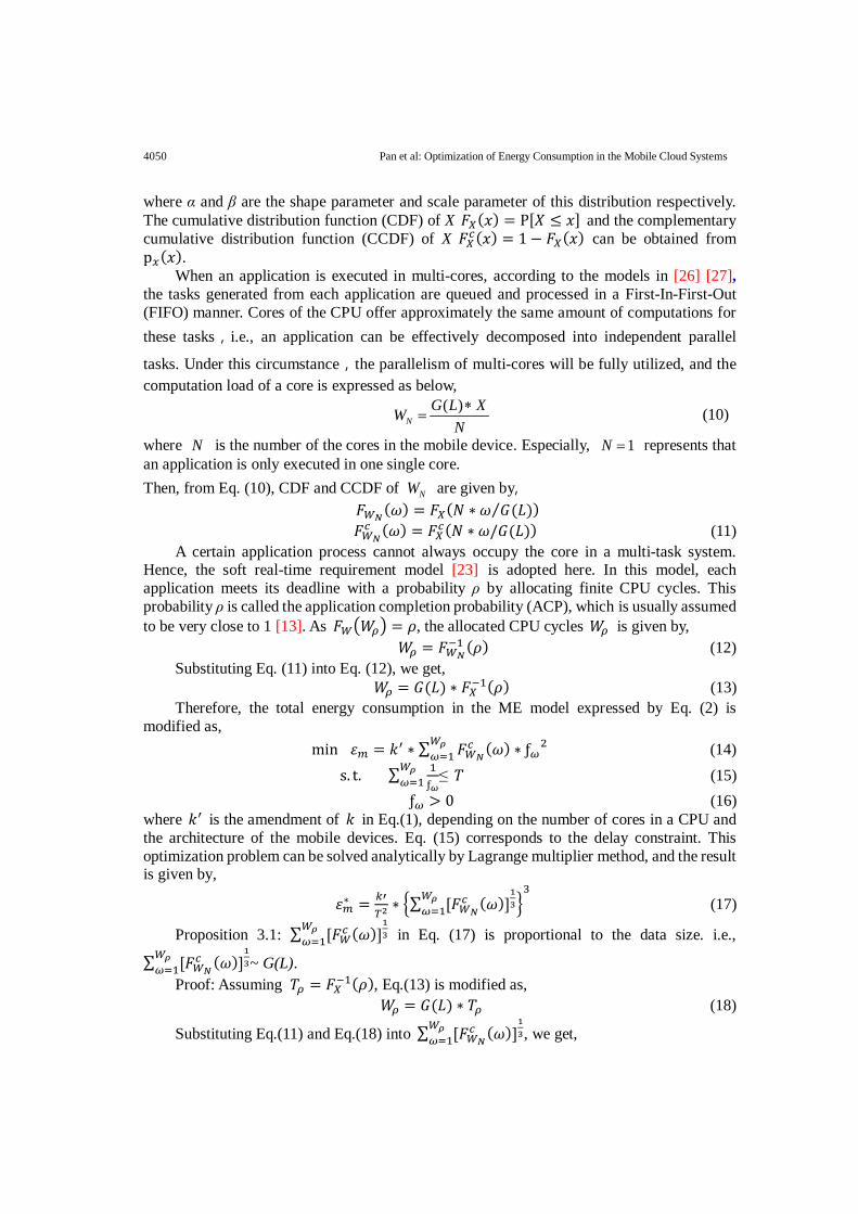
4050 Pan et al: Optimization of Energy Consumption in the Mobile Cloud Systems
where α and β are the shape parameter and scale parameter of this distribution respectively. The cumulative distribution function (CDF) of X 𝐹𝑋(𝑥) = P[𝑋 ≤ 𝑥] and the complementary cumulative distribution function (CCDF) of X 𝐹𝑋𝑐(𝑥) = 1− 𝐹𝑋(𝑥) can be obtained from p𝑥(𝑥).
When an application is executed in multi-cores, according to the models in [26] [27], the tasks generated from each application are queued and processed in a First-In-First-Out (FIFO) manner. Cores of the CPU offer approximately the same amount of computations for these tasks,i.e., an application can be effectively decomposed into independent parallel
tasks. Under this circumstance,the parallelism of multi-cores will be fully utilized, and the computation load of a core is expressed as below,
( )N
G L XWN∗
= (10)
where N is the number of the cores in the mobile device. Especially, 1N = represents that an application is only executed in one single core. Then, from Eq. (10), CDF and CCDF of NW are given by,
𝐹𝑊𝑁(𝜔) = 𝐹𝑋(𝑁 ∗ 𝜔 𝐺(𝐿)⁄ )
𝐹𝑊𝑁𝑐 (𝜔) = 𝐹𝑋𝑐(𝑁 ∗ 𝜔/𝐺(𝐿)) (11)
A certain application process cannot always occupy the core in a multi-task system. Hence, the soft real-time requirement model [23] is adopted here. In this model, each application meets its deadline with a probability ρ by allocating finite CPU cycles. This probability ρ is called the application completion probability (ACP), which is usually assumed to be very close to 1 [13]. As 𝐹𝑊�𝑊𝜌� = 𝜌, the allocated CPU cycles 𝑊𝜌 is given by,
𝑊𝜌 = 𝐹𝑊𝑁−1 (𝜌) (12)
Substituting Eq. (11) into Eq. (12), we get, 𝑊𝜌 = 𝐺(𝐿) ∗ 𝐹𝑋−1(𝜌) (13)
Therefore, the total energy consumption in the ME model expressed by Eq. (2) is modified as,
min 𝜀𝑚 = 𝑘′ ∗ ∑ 𝐹𝑊𝑁𝑐 (𝜔) ∗ ƒ𝜔
2𝑊𝜌𝜔=1 (14)
s. t. ∑ 1ƒ𝜔
𝑊𝜌𝜔=1 ≤ 𝑇 (15)
ƒ𝜔 > 0 (16) where 𝑘′ is the amendment of 𝑘 in Eq.(1), depending on the number of cores in a CPU and the architecture of the mobile devices. Eq. (15) corresponds to the delay constraint. This optimization problem can be solved analytically by Lagrange multiplier method, and the result is given by,
𝜀𝑚∗ = 𝑘′𝑇2∗ �∑ [𝐹𝑊𝑁
𝑐 (𝜔)]13
𝑊𝜌𝜔=1 �
3 (17)
Proposition 3.1: ∑ [𝐹𝑊𝑐 (𝜔)]13
𝑊𝜌𝜔=1 in Eq. (17) is proportional to the data size. i.e.,
∑ [𝐹𝑊𝑁𝑐 (𝜔)]
13
𝑊𝜌𝜔=1 ~ G(L).
Proof: Assuming 𝑇𝜌 = 𝐹𝑋−1(𝜌), Eq.(13) is modified as, 𝑊𝜌 = 𝐺(𝐿) ∗ 𝑇𝜌 (18)
Substituting Eq.(11) and Eq.(18) into ∑ [𝐹𝑊𝑁𝑐 (𝜔)]
13
𝑊𝜌𝜔=1 , we get,
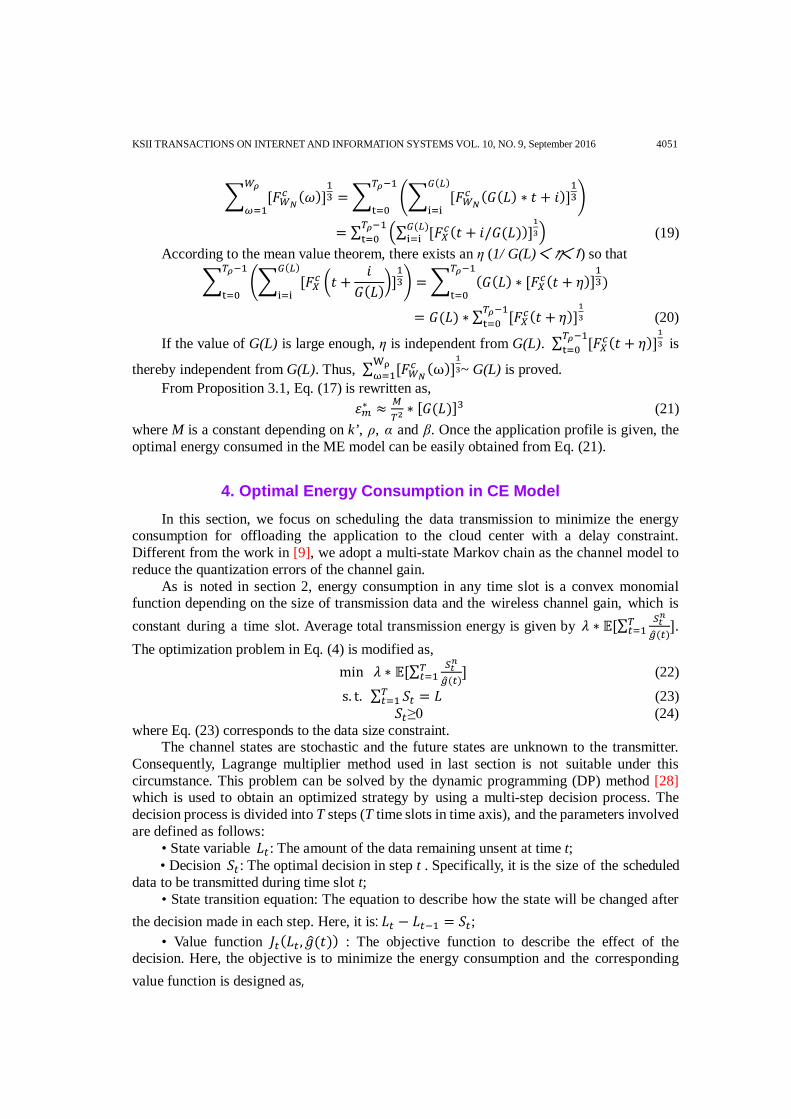
KSII TRANSACTIONS ON INTERNET AND INFORMATION SYSTEMS VOL. 10, NO. 9, September 2016 4051
� [𝐹𝑊𝑁𝑐 (𝜔)]
13
𝑊𝜌
𝜔=1= � �� [𝐹𝑊𝑁
𝑐 (𝐺(𝐿) ∗ 𝑡 + 𝑖)]13
𝐺(𝐿)
i=i�
𝑇𝜌−1
t=0
= ∑ �∑ [𝐹𝑋𝑐(𝑡 + 𝑖/𝐺(𝐿))]13
𝐺(𝐿)i=i �𝑇𝜌−1
t=0 (19) According to the mean value theorem, there exists an η (1/ G(L)<η<1) so that
� �� [𝐹𝑋𝑐 �𝑡 +𝑖
𝐺(𝐿)�]13
𝐺(𝐿)
i=i�
𝑇𝜌−1
t=0= � (𝐺(𝐿) ∗ [𝐹𝑋𝑐(𝑡 + 𝜂)]
13)
𝑇𝜌−1
t=0
= 𝐺(𝐿) ∗ ∑ [𝐹𝑋𝑐(𝑡 + 𝜂)]13
𝑇𝜌−1t=0 (20)
If the value of G(L) is large enough, η is independent from G(L). ∑ [𝐹𝑋𝑐(𝑡 + 𝜂)]13
𝑇𝜌−1t=0 is
thereby independent from G(L). Thus, ∑ [𝐹𝑊𝑁𝑐 (ω)]
13
Wρω=1 ~ G(L) is proved.
From Proposition 3.1, Eq. (17) is rewritten as, 𝜀𝑚∗ ≈ 𝑀
𝑇2∗ [𝐺(𝐿)]3 (21)
where M is a constant depending on k’, ρ, α and β. Once the application profile is given, the optimal energy consumed in the ME model can be easily obtained from Eq. (21).
4. Optimal Energy Consumption in CE Model In this section, we focus on scheduling the data transmission to minimize the energy
consumption for offloading the application to the cloud center with a delay constraint. Different from the work in [9], we adopt a multi-state Markov chain as the channel model to reduce the quantization errors of the channel gain.
As is noted in section 2, energy consumption in any time slot is a convex monomial function depending on the size of transmission data and the wireless channel gain, which is constant during a time slot. Average total transmission energy is given by 𝜆 ∗ 𝔼[∑ 𝑆𝑡𝑛
𝑔�(𝑡)𝑇𝑡=1 ].
The optimization problem in Eq. (4) is modified as, min 𝜆 ∗ 𝔼[∑ 𝑆𝑡𝑛
𝑔�(𝑡)𝑇𝑡=1 ] (22)
s. t. ∑ 𝑆𝑡 = 𝐿𝑇𝑡=1 (23) 𝑆𝑡≥0 (24)
where Eq. (23) corresponds to the data size constraint. The channel states are stochastic and the future states are unknown to the transmitter.
Consequently, Lagrange multiplier method used in last section is not suitable under this circumstance. This problem can be solved by the dynamic programming (DP) method [28] which is used to obtain an optimized strategy by using a multi-step decision process. The decision process is divided into T steps (T time slots in time axis), and the parameters involved are defined as follows:
• State variable 𝐿𝑡: The amount of the data remaining unsent at time t; • Decision 𝑆𝑡: The optimal decision in step t . Specifically, it is the size of the scheduled
data to be transmitted during time slot t; • State transition equation: The equation to describe how the state will be changed after
the decision made in each step. Here, it is: 𝐿𝑡 − 𝐿𝑡−1 = 𝑆𝑡; • Value function 𝐽𝑡(𝐿𝑡 ,𝑔�(𝑡)) : The objective function to describe the effect of the
decision. Here, the objective is to minimize the energy consumption and the corresponding value function is designed as,
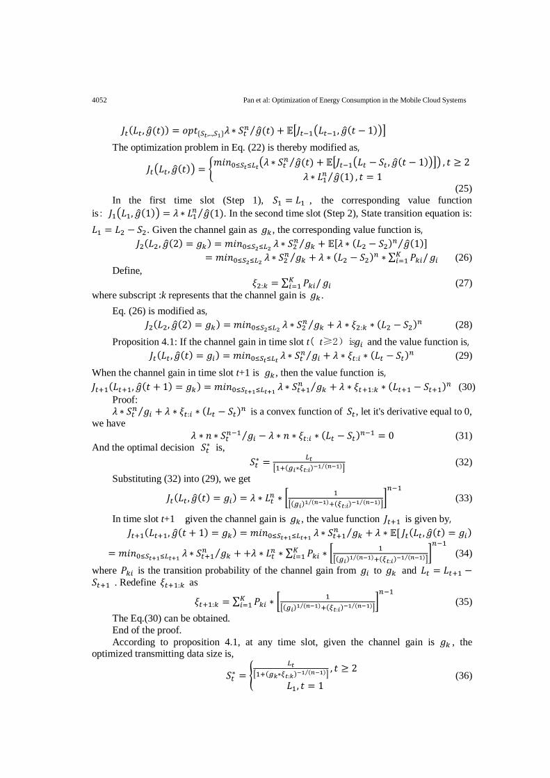
4052 Pan et al: Optimization of Energy Consumption in the Mobile Cloud Systems
𝐽𝑡(𝐿𝑡 ,𝑔�(𝑡)) = 𝑜𝑝𝑡{𝑆𝑡,..,𝑆1}𝜆 ∗ 𝑆𝑡𝑛 𝑔�(𝑡)⁄ + 𝔼�𝐽𝑡−1�𝐿𝑡−1 ,𝑔�(𝑡 − 1)�� The optimization problem in Eq. (22) is thereby modified as,
𝐽𝑡�𝐿𝑡,𝑔�(𝑡)� = �𝑚𝑖𝑛0≤𝑆𝑡≤𝐿𝑡�𝜆 ∗ 𝑆𝑡𝑛 𝑔�(𝑡)⁄ + 𝔼�𝐽𝑡−1�𝐿𝑡 − 𝑆𝑡 ,𝑔�(𝑡 − 1)��� , 𝑡 ≥ 2
𝜆 ∗ 𝐿1𝑛 𝑔�(1)⁄ , 𝑡 = 1�
(25) In the first time slot (Step 1), 𝑆1 = 𝐿1 , the corresponding value function
is: 𝐽1�𝐿1,𝑔�(1)� = 𝜆 ∗ 𝐿1𝑛 𝑔�(1)⁄ . In the second time slot (Step 2), State transition equation is: 𝐿1 = 𝐿2 − 𝑆2. Given the channel gain as 𝑔𝑘 , the corresponding value function is,
𝐽2(𝐿2 ,𝑔�(2) = 𝑔𝑘) = 𝑚𝑖𝑛0≤𝑆2≤𝐿2 𝜆 ∗ 𝑆2𝑛 𝑔𝑘⁄ + 𝔼[𝜆 ∗ (𝐿2 − 𝑆2)𝑛 𝑔�(1)⁄ ]
= 𝑚𝑖𝑛0≤𝑆2≤𝐿2 𝜆 ∗ 𝑆2𝑛 𝑔𝑘⁄ + 𝜆 ∗ (𝐿2 − 𝑆2)𝑛 ∗ ∑ 𝑃𝑘𝑖/𝐾
𝑖=1 𝑔𝑖 (26) Define,
𝜉2:𝑘 = ∑ 𝑃𝑘𝑖/𝐾𝑖=1 𝑔𝑖 (27)
where subscript :k represents that the channel gain is 𝑔𝑘 . Eq. (26) is modified as,
𝐽2(𝐿2,𝑔�(2) = 𝑔𝑘) = 𝑚𝑖𝑛0≤𝑆2≤𝐿2 𝜆 ∗ 𝑆2𝑛 𝑔𝑘⁄ + 𝜆 ∗ 𝜉2:𝑘 ∗ (𝐿2 − 𝑆2)𝑛 (28)
Proposition 4.1: If the channel gain in time slot t( t≥2)is 𝑔𝑖 and the value function is, 𝐽𝑡(𝐿𝑡 ,𝑔�(𝑡) = 𝑔𝑖) = 𝑚𝑖𝑛0≤𝑆𝑡≤𝐿𝑡 𝜆 ∗ 𝑆𝑡
𝑛 𝑔𝑖⁄ + 𝜆 ∗ 𝜉𝑡:𝑖 ∗ (𝐿𝑡 − 𝑆𝑡)𝑛 (29)
When the channel gain in time slot t+1 is 𝑔𝑘 , then the value function is, 𝐽𝑡+1(𝐿𝑡+1,𝑔�(𝑡 + 1) = 𝑔𝑘) = 𝑚𝑖𝑛0≤𝑆𝑡+1≤𝐿𝑡+1 𝜆 ∗ 𝑆𝑡+1
𝑛 𝑔𝑘⁄ + 𝜆 ∗ 𝜉𝑡+1:𝑘 ∗ (𝐿𝑡+1 − 𝑆𝑡+1)𝑛 (30) Proof: 𝜆 ∗ 𝑆𝑡𝑛 𝑔𝑖⁄ + 𝜆 ∗ 𝜉𝑡:𝑖 ∗ (𝐿𝑡 − 𝑆𝑡)𝑛 is a convex function of 𝑆𝑡 , let it's derivative equal to 0,
we have 𝜆 ∗ 𝑛 ∗ 𝑆𝑡𝑛−1 𝑔𝑖⁄ − 𝜆 ∗ 𝑛 ∗ 𝜉𝑡:𝑖 ∗ (𝐿𝑡 − 𝑆𝑡)𝑛−1 = 0 (31)
And the optimal decision 𝑆𝑡∗ is, 𝑆𝑡∗ = 𝐿𝑡
�1+(𝑔𝑖∗𝜉𝑡:𝑖)−1 (𝑛−1)⁄ � (32) Substituting (32) into (29), we get
𝐽𝑡(𝐿𝑡 ,𝑔�(𝑡) = 𝑔𝑖) = 𝜆 ∗ 𝐿𝑡𝑛 ∗ �1
�(𝑔𝑖)1 (𝑛−1)⁄ +(𝜉𝑡:𝑖)−1 (𝑛−1)⁄ ��𝑛−1
(33)
In time slot t+1 ,given the channel gain is 𝑔𝑘 , the value function 𝐽𝑡+1 is given by, 𝐽𝑡+1(𝐿𝑡+1,𝑔�(𝑡 + 1) = 𝑔𝑘) = 𝑚𝑖𝑛0≤𝑆𝑡+1≤𝐿𝑡+1 𝜆 ∗ 𝑆𝑡+1
𝑛 𝑔𝑘⁄ + 𝜆 ∗ 𝔼[ 𝐽𝑡(𝐿𝑡 ,𝑔�(𝑡) = 𝑔𝑖)
= 𝑚𝑖𝑛0≤𝑆𝑡+1≤𝐿𝑡+1 𝜆 ∗ 𝑆𝑡+1𝑛 𝑔𝑘⁄ + +𝜆 ∗ 𝐿𝑡𝑛 ∗ ∑ 𝑃𝑘𝑖 ∗ �
1�(𝑔𝑖)1 (𝑛−1)⁄ +(𝜉𝑡:𝑖)−1 (𝑛−1)⁄ �
�𝑛−1
𝐾𝑖=1 (34)
where 𝑃𝑘𝑖 is the transition probability of the channel gain from 𝑔𝑖 to 𝑔𝑘 and 𝐿𝑡 = 𝐿𝑡+1 −𝑆𝑡+1 . Redefine 𝜉𝑡+1:𝑘 as
𝜉𝑡+1:𝑘 = ∑ 𝑃𝑘𝑖 ∗ �1
�(𝑔𝑖)1 (𝑛−1)⁄ +(𝜉𝑡:𝑖)−1 (𝑛−1)⁄ ��𝑛−1
𝐾𝑖=1 (35)
The Eq.(30) can be obtained. End of the proof. According to proposition 4.1, at any time slot, given the channel gain is 𝑔𝑘 , the
optimized transmitting data size is,
𝑆𝑡∗ = �𝐿𝑡
�1+(𝑔𝑘∗𝜉𝑡:𝑘)−1 (𝑛−1)⁄ � , 𝑡 ≥ 2
𝐿1 , 𝑡 = 1� (36)
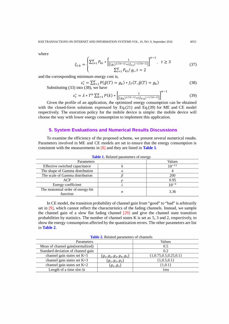
KSII TRANSACTIONS ON INTERNET AND INFORMATION SYSTEMS VOL. 10, NO. 9, September 2016 4053
where
𝜉𝑡:𝑘 = �∑ 𝑃𝑘𝑖 ∗ �1
�(𝑔𝑖)1 (𝑛−1)⁄ +(𝜉𝑡:𝑖)−1 (𝑛−1)⁄ ��𝑛−1,𝑡 ≥ 3𝐾
𝑖=1
∑ 𝑃𝑘𝑖/𝐾𝑖=1 𝑔𝑖 , 𝑡 = 2
� (37)
and the corresponding minimum energy cost is, 𝜀𝑐∗ = ∑ P(𝑔�(𝑇) = 𝑔𝑘) ∗ 𝐽𝑇(𝑇,𝑔�(𝑇) = 𝑔𝑘)𝐾
𝑘=1 (38) Substituting (33) into (38), we have
𝜀𝑐∗ = 𝜆 ∗ 𝑇𝑛 ∑ 𝑃(𝑘) ∗ � 1�(𝑔𝑘)1 (𝑛−1)⁄ +(𝜉𝑇:𝑘)−1 (𝑛−1)⁄ �
�𝑛−1
𝐾𝑘=1 (39)
Given the profile of an application, the optimized energy consumption can be obtained with the closed-form solutions expressed by Eq.(21) and Eq.(39) for ME and CE model respectively. The execution policy for the mobile device is simple: the mobile device will choose the way with lower energy consumption to implement this application.
5. System Evaluations and Numerical Results Discussions To examine the efficiency of the proposed scheme, we present several numerical results.
Parameters involved in ME and CE models are set to ensure that the energy consumption is consistent with the measurements in [8] and they are listed in Table 1.
Table 1. Related parameters of energy
Parameters Values Effective switched capacitance k 10−11
The shape of Gamma distribution α 4 The scale of Gamma distribution β 200
ACP ρ 0.95 Energy coefficient λ 10−3
The monomial order of energy-bit function n 3.36
In CE model, the transition probability of channel gain from “good” to “bad” is arbitrarily
set in [9], which cannot reflect the characteristics of the fading channels. Instead, we sample the channel gain of a slow flat fading channel [29] and give the channel state transition probabilities by statistics. The number of channel states K is set as 5, 3 and 2, respectively, to show the energy consumption affected by the quantization errors. The other parameters are list in Table 2.
Table 2. Related parameters of channels
Parameters Values Mean of channel gain(normalized) 0.5 Standard deviation of channel gain 0.2
channel gain states set K=5 {𝑔1,𝑔2,𝑔3,𝑔4,𝑔5} {1,0.75,0.5,0.25,0.1} channel gain states set K=3 {𝑔1,𝑔2,𝑔3} {1,0.5,0.1} channel gain states set K=2 {𝑔1,𝑔2} {1,0.1}
Length of a time slot Δt 1ms

4054 Pan et al: Optimization of Energy Consumption in the Mobile Cloud Systems
Fig. 2. Normalized Channel gain and the quantized values
Table 3. Statistical results of the transition probability metric in K=5
j=1 j=2 j=3 j=4 j=5 i=1 0.5769 0.4231 0 0 0 i=2 0.0340 0.8565 0.1058 0.0037 0 i=3 0.0036 0.2049 0.6774 0.1123 0.0018 i=4 0 0.0053 0.3413 0.4933 0.1600 i=5 0 0 0.0219 0.3115 0.6667
As stated earlier, we adopt a multi-state Markov model to describe the stochastic changes
of slow fading wireless channels. Fig. 2 (a) shows the normalized channel gain of slow fading wireless channels, which is log-normal distributed in our simulations. And Fig. 2 (b) demonstrates the quantized value when we sampled the corresponding normalized channel gain with 5 scales, i.e., 5 channel states. Compared with the dual-state Markov method in [9], where the channel gain was quantized in “good” and “bad” states, our multi-state Markov method better reflects the stochastic feature of the fading channel and can be helpful in increasing the accuracy of energy optimization algorithm.
Table. 3 displays the channel states transition probabilities 𝑃𝑖𝑗 by statistical analysis of the channel gain values in Fig. 2 (b). 𝑃𝑖𝑗 is used in dynamic transmission data scheduling algorithm to minimize energy consumption for offloading the application to the cloud center.

KSII TRANSACTIONS ON INTERNET AND INFORMATION SYSTEMS VOL. 10, NO. 9, September 2016 4055
5.1 Performance of Mobile Execution Energy Model The energy consumed by three different applications executed in ME model is given in
Fig. 3 with the application completion deadline T as 40 milliseconds. These three applications are all in algorithm level, with their ATC given in Table 4. As demonstrated in Fig. 3, it is obvious that the energy cost increases with the size of the data, and the growth rate is proportional to the ATC of the application. The reason is that the second-order partial derivative of the energy in Eq. (21) with respect to the G(L) is greater than zero, and the G(L) increases with the ATC. Consequently, the energy gaps among applications grow with the data size which means that the higher complexity application cost much more energy than the lower complexity ones as the data size rises. We also find in Fig. 3 that the energy consumption in a two-core CPU is lower than that in a single-core CPU. This is because given a fixed deadline, the computation load is distributed among two cores, so the clock frequency of each core can be lower than that of the single-core CPU. It results in the lower energy consumption according to Eq.(1).
Table 4. Algorithm level applications and their time complexity
Applications ATC binary search log(m) order search m merge sort m×log(m)
0 500 1000 1500 2000 2500 3000 3500 400010
-2
100
102
104
106
108
data size L(bits) T=40ms
Ene
rgy
cons
umpt
ion
E(u
J)
Binary search in ME, single coreBinary search in ME, multi-core N=2
Order search in ME, single core
Order search in ME, multi-core N=2Merge sort in ME, single core
Merge sort in ME, multi-core N=2
Fig. 3. Energy consumed (in logs) by mobile device versus the input data size L
4056 Pan et al: Optimization of Energy Consumption in the Mobile Cloud Systems
5.2 Performance of Cloud Execution Energy Model This subsection describes the analytical and simulation results of CE model and presents
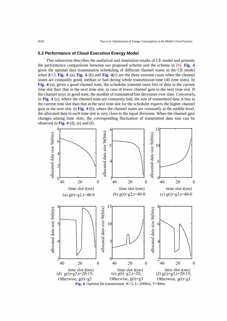
the performance comparisons between our proposed scheme and the scheme in [9]. Fig. 4 gives the optimal data transmission scheduling of different channel states in the CE model when K=3. Fig. 4 (a), Fig. 4 (b) and Fig. 4(c) are the three extreme cases when the channel states are constantly good, median or bad during whole transmission time (40 time slots). In Fig. 4 (a), given a good channel state, the scheduler transmit more bits of data in the current time slot than that in the next time slot, in case of lower channel gain in the next time slot. If the channel stays in good state, the number of transmitted bits decreases over time. Conversely, in Fig. 4 (c), where the channel state are constantly bad, the size of transmitted data is less in the current time slot than that in the next time slot for the scheduler expects the higher channel gain in the next slot. In Fig. 4 (b), where the channel states are constantly at the middle level, the allocated data in each time slot is very close to the equal divisions. When the channel gain changes among time slots, the corresponding fluctuation of transmitted data size can be observed in Fig. 4 (d), (e) and (f).
Fig. 4. Optimal bit transmission, K=3, L=200bits, T=40ms
KSII TRANSACTIONS ON INTERNET AND INFORMATION SYSTEMS VOL. 10, NO. 9, September 2016 4057
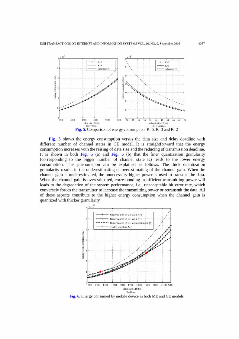
Fig. 5. Comparison of energy consumption, K=5, K=3 and K=2
Fig. 5 shows the energy consumption versus the data size and delay deadline with
different number of channel states in CE model. It is straightforward that the energy consumption increases with the raising of data size and the reducing of transmission deadline. It is shown in both Fig. 5 (a) and Fig. 5 (b) that the finer quantization granularity (corresponding to the bigger number of channel state K) leads to the lower energy consumption. This phenomenon can be explained as follows. The thick quantization granularity results in the underestimating or overestimating of the channel gain. When the channel gain is underestimated, the unnecessary higher power is used to transmit the data. When the channel gain is overestimated, corresponding insufficient transmitting power will leads to the degradation of the system performance, i.e., unacceptable bit error rate, which conversely forces the transmitter to increase the transmitting power or retransmit the data. All of these aspects contribute to the higher energy consumption when the channel gain is quantized with thicker granularity.
Fig. 6. Energy consumed by mobile device in both ME and CE models
4058 Pan et al: Optimization of Energy Consumption in the Mobile Cloud Systems
Finally, we analyze the execution policy of the mobile device. Energy consumed by the mobile device for a given application, e.g., "order search", is plot in Fig. 6.The energy consumption increases with the data size in both ME and CE models. When the data size is small (below the highlight points in Fig. 6), the energy consumption in ME model is smaller than that in CE model, the mobile device is thereby inclined to offload the application to the cloud center to save the energy. Otherwise, the mobile device executes the application locally. It is noted that when the 5-channel-states (K=5) scheme is used, the mobile device will offloads the application to the cloud with the data size below 1900, while the corresponding data size in the scheme [9] is around 1350 (referring to the highlight points in Fig. 6). It means that the quantization granularity (corresponding to the number of channel states) can affect the choosing behaviors of the mobile devices. Comparing to the 5-channel-states (K=5) scheme, the dual channel states scheme used in [9] leads to the higher transmission energy cost and hinders the mobile device to save energy by utilizing application offloading.
6. Conclusion In this paper we investigate the problem of optimizing the energy consumption of mobile
devices in the Mobile Computing Cloud environment. We distinguish the applications’ computational requirements to optimize the energy consumed by CPUs in mobile devices by introducing the asymptotic time complexity (ATC) method. We propose a multi-scale scheme to quantize the channel gain, which better reveals the stochastic feature of wireless fading channel compared with the dual-state Markov method in [9]. Our proposed multi-scale scheme is proved to be helpful for reducing the energy consumed by mobile devices when offloading the applications to the cloud center. Besides, our analytical results can also be used as a guideline for the mobile devices to decide either executing the application locally or offloading it to the cloud center. It is noted that we only consider the scenario where an application is fully parallelism available while neglecting the scheduling cost in multi-core mobile execution model. Our future work will consider the parallel scheduling algorithms for the asymmetric multi-core architecture CPUs and improve the estimation accuracy of energy consumption in the ME model.
APPENDIX A The monomial order n in Eq.(3) ranges from 2 to 5, which is related to the transmission
mode (including both the modulation and coding scheme). The value of n can be obtained from the best (least-square) approximation of 𝜀𝑐(𝑆𝑡 ,𝑔(𝑡)) to the form 𝜆 × 𝑆𝑡𝑛
𝑔(𝑡) [19].
Usually, the transmission mode is determined according to the bit-error rate requirements of the wireless system. We use a practical system as an example to illustrate the problem. The transmission modes for the OFDM system using adaptive modulation and coding (AMC) are shown in Table 5, which have been adopted by 802.11a standard [30].
KSII TRANSACTIONS ON INTERNET AND INFORMATION SYSTEMS VOL. 10, NO. 9, September 2016 4059
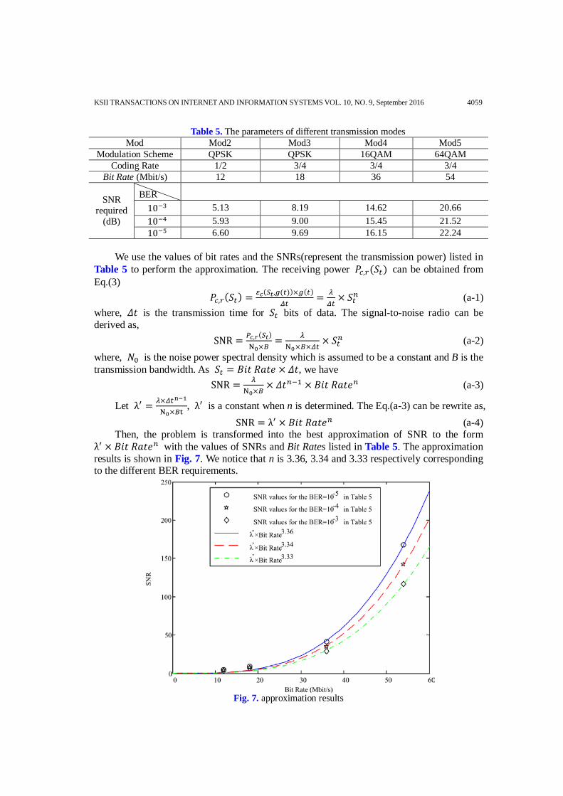
Table 5. The parameters of different transmission modes Mod Mod2 Mod3 Mod4 Mod5
Modulation Scheme QPSK QPSK 16QAM 64QAM Coding Rate 1/2 3/4 3/4 3/4
Bit Rate (Mbit/s) 12 18 36 54
SNR required
(dB)
BER
10−3 5.13 8.19 14.62 20.66 10−4 5.93 9.00 15.45 21.52 10−5 6.60 9.69 16.15 22.24
We use the values of bit rates and the SNRs(represent the transmission power) listed in
Table 5 to perform the approximation. The receiving power 𝑃𝑐,𝑟(𝑆𝑡) can be obtained from Eq.(3)
𝑃𝑐,𝑟(𝑆𝑡) = 𝜀𝑐(𝑆𝑡,𝑔(𝑡))×𝑔(𝑡)𝛥𝑡
= 𝜆𝛥𝑡
× 𝑆𝑡𝑛 (a-1) where, 𝛥𝑡 is the transmission time for 𝑆𝑡 bits of data. The signal-to-noise radio can be derived as,
SNR = 𝑃𝑐,𝑟(𝑆𝑡)N0×𝐵
= 𝜆N0×𝐵×𝛥𝑡
× 𝑆𝑡𝑛 (a-2) where, 𝑁0 is the noise power spectral density which is assumed to be a constant and B is the transmission bandwidth. As 𝑆𝑡 = 𝐵𝑖𝑡 𝑅𝑎𝑡𝑒 × 𝛥𝑡, we have
SNR = 𝜆N0×𝐵
× 𝛥𝑡𝑛−1 × 𝐵𝑖𝑡 𝑅𝑎𝑡𝑒𝑛 (a-3)
Let λ′ = 𝜆×𝛥𝑡n−1
N0×𝐵t, λ′ is a constant when n is determined. The Eq.(a-3) can be rewrite as,
SNR = λ′ × 𝐵𝑖𝑡 𝑅𝑎𝑡𝑒𝑛 (a-4) Then, the problem is transformed into the best approximation of SNR to the form
λ′ × 𝐵𝑖𝑡 𝑅𝑎𝑡𝑒𝑛 with the values of SNRs and Bit Rates listed in Table 5. The approximation results is shown in Fig. 7. We notice that n is 3.36, 3.34 and 3.33 respectively corresponding to the different BER requirements.
Fig. 7. approximation results
4060 Pan et al: Optimization of Energy Consumption in the Mobile Cloud Systems
Acknowledgments
This work was supported by the National Natural Science Foundation of China (No.61271235), and A Project Funded by the Priority Academic Program Development of Jiangsu Higher Education Institutions——Information and Communication Engineering.
References [1] M. Rahman, J. Gao and T. Wei-Tek, “Energy saving in mobile cloud computing,” in Proc. of IEEE
International Conference on Cloud Engineering, pp. 285-291, 2013. Article (CrossRef Link) [2] P. B. Si, Q. Zhang, F. R. Yu and Y. H. Zhang, “QoS-aware dynamic resource management in
heterogeneous mobile cloud computing networks,” China Communications, vol. 11, no. 5, pp. 144-159, 2014. Article (CrossRef Link)
[3] R. Kumer and S. Rajalakshmi, “Mobile Cloud Computing: Standard Approach to Protecting and Securing of Mobile Cloud Ecosystems,” in Proc. of International Conference on Computer Sciences and Applications, pp. 663-669, 2013. Article (CrossRef Link)
[4] D. Dev and K. L. Baishnab, “A Review and Research Towards Mobile Cloud Computing,” in Proc. of IEEE International Conference on Mobile Cloud Computing, Services, and Engineering (MobileCloud), pp. 252-256, 2014. Article (CrossRef Link)
[5] S. Barbarossa, P. Di Lorenzo, and S. Sardellitti, “Computation Offloading Strategies based on Energy Minimization under Computational Rate Constraints,” in Proc. of European Conference on Networks and Communications (EuCNC), pp. 1-5, 2014. Article (CrossRef Link)
[6] W. Lee, J. Jung and H. Kim, “Analyzing Extent and Influence of Mobile Device’s Participation in Mobile Cloud Computing,” in Proc. of ICT Convergence (ICTC), pp. 767-772, 2013. Article (CrossRef Link)
[7] K. Kumar and Y. H. Lu, “Cloud computing for mobile users: can offloading computation save energy?” IEEE Computer, vol. 43, no. 4, pp. 51–56, 2010. Article (CrossRef Link)
[8] A. P. Miettinen and J. K. Nurminen, “Energy efficiency of mobile clients in cloud computing,” in Proc. of 2010 USENIX conference on hot topics in cloud computing. Article (CrossRef Link)
[9] W. W. Zhang, Y. G. Wen and K. Guan, “Energy-Optimal Mobile Cloud Computing under Stochastic Wireless Channel,” IEEE Transaction on Wireless Communications, vol. 12, no. 9, pp. 4569-4581, 2013. Article (CrossRef Link)
[10] Clifford A. Shaffer, A practical introduction to data structures and algorithm analysis, Edition 3.2 (C++ Version), Blacksburg, VA, 2011. Article (CrossRef Link)
[11] B. Liu, L. M. Du and L. Y. Xie, “Performance analysis of embedded speech recognition system,” in Proc. of Microcomputer applications, vol. 29, no. 7, pp. 52-55, 2008. Article (CrossRef Link)
[12] T. Burd and R. Broderson, “Processor design for portable systems,” J. VLSI Singapore Process, vol. 13, no. 2, pp. 203–222, 1996. Article (CrossRef Link)
[13] M. Yang, Y. G. Wen, J. F. Cai and C. H. Foh, “Energy Minimization via Dynamic Voltage Scaling for Real-Time Video Encoding on Mobile Devices,” in Proc. of IEEE International Conference on Communications (ICC), pp. 2026-2031, 2012. Article (CrossRef Link)
[14] J. M. Rabaey, Digital Integrated Circuits, Prentice Hall, 1996. Article (CrossRef Link) [15] Y. Chen, S. Q. Zhang and G. Y. Li, “Fundamental trade-offs on green wireless networks,” IEEE
Communication Magazine, vol. 49, no. 6, pp. 30–37, 2011. Article (CrossRef Link) [16] R. A. Berry and R. G. Gallager, “Communication over fading channels with delay constraints,” in
Proc. of IEEE Transaction on Information Theory, vol. 48, no.5, pp. 1135-1149, 2002. Article (CrossRef Link)
[17] E. Uysal and G. A. Ei, “On Adaptive transmission for energy-efficiency in wireless data networks,” IEEE Transaction on Information Theory, vol. 50, no. 12, pp. 3081-3094, 2004. Article (CrossRef Link)
KSII TRANSACTIONS ON INTERNET AND INFORMATION SYSTEMS VOL. 10, NO. 9, September 2016 4061
[18] J. Lee and N. Jindal, “Energy-efficient scheduling of delay constrained traffic over fading channels,” IEEE Transaction on Wireless Communication, vol. 8, no. 4, pp. 1866–1875, 2009. Article (CrossRef Link)
[19] Z. F. Murtaza and M. Eytan, “Minimum Energy Transmission over a Wireless Fading Channel with Packet Deadlines,” in Proc. of IEEE Conference on Decision and Control, pp. 1148-1155, 2007. Article (CrossRef Link)
[20] P. Rong and M. Redram, “Extending the lifetime of a Network of battery-powered mobile devices by remote processing: a Markova decision-based approach,” in Proc. of IEEE Design Automation Conference, pp. 906-911, 2003. Article (CrossRef Link)
[21] M. Zorzi, R. R. Rao and L. B. Milstein, “Error statistics in data transmission over fading channels,” IEEE Transactions on Communications, vol. 46, no. 11, pp. 1468-1477, 1998. Article (CrossRef Link)
[22] B. Ahmed and S. Buonomo, “Simulation of 20 GHz Narrow Band Mobile Propagation Data Using N-States Markov Channel Modeling Approach,” in Proc. of Tenth International Conference on Antennas and Propagation, vol. 2, pp. 48-53, 1997. Article (CrossRef Link)
[23] W. H. Yuan and K. Nahrstedt, “Energy-efficient soft real-time CPU scheduling for mobile multimedia applications,” ACM Trans. Computer System, vol. 24, no. 3, pp. 292–331, 2003. Article (CrossRef Link)
[24] Q. Li, B. Guo, Y. Shen and J. H. Wang, “An embedded software power model on algorithm complexity using back-propagation neural networks,” in Proc. of IEEE/ACM international Conference on Green Computing and Communications, pp. 454-459, 2010. Article (CrossRef Link)
[25] Y. W. Choi, M. Khan, V. S. A. Kumar and G. Pandurangan, “Energy-optimal distributed algorithms for minimum spanning trees,” IEEE Journal on Selected Areas in Communications, vol. 27, no. 7, pp. 1297-1304, 2009. Article (CrossRef Link)
[26] Z. Jiang and S. Mao, "Energy Delay Trade-Off in Cloud Offloading for Mutli-Core Mobile Devices," in Proc. of 2015 IEEE Global Communications Conference (GLOBECOM), San Diego, CA, pp. 1-6, 2015. Article (CrossRef Link)
[27] Z. Jiang and S. Mao, "Energy Delay Tradeoff in Cloud Offloading for Multi-Core Mobile Devices," in Proc. of IEEE Access, vol. 3, no. , pp. 2306-2316, 2015. Article (CrossRef Link)
[28] S. Moshe, Dynamic Programming: Foundations and Principles, CRC Press Inc, 2010. Article (CrossRef Link)
[29] H. C. Yang and M. S. Alouini, “A hierarchical Markov model for wireless shadowed fading channels,” in Proc. of IEEE Vehicular Technology Conference, vol. 2, pp. 640-644, 2002. Article (CrossRef Link)
[30] Z. H. Guo, P. Zhang and H. Harada, “A Crosslayer Design with power control and AMC for Sub-band Based OFDM System,” in Proc. of IEEE Conference on Communications and Networking in China, 1-6, 2006. Article (CrossRef Link)
4062 Pan et al: Optimization of Energy Consumption in the Mobile Cloud Systems
Pan Su is a Professor in the Faculty of Telecommunication Engineering of Nanjing University of Posts and Telecommunications, China. He received his Bachelor degrees of Engineering from Huazhong University of Science and Technology, China and his Master of Engineering degree, from Nanjing University of Posts and Telecommunications Nanjing, China. After graduation, he held appointment in Motorola, Inc. and obtained the Training Instructor Certification in Chicago, US. in 1995. He obtained his Ph. D. degree in electrical and electronic engineering from The University of Hong Kong, Hong Kong in 2004. Since August 2004, he has been with the Nanjing University of Posts and Telecommunications. Professor Pan has published more than 40 papers in journals and conferences. His research interests are in the general areas of wireless communications, particularly, wireless resource allocation and QoS guarantee in OFDM, MIMO and heterogeneous networks.
Wang Shengping received his B.Sc. degree in North China Electric Power University, and received his Master’s degree in Nanjing University of Posts and Telecommunications. He is currently working as an assistant engineer in Jiangsu Power Design Institute Co., Ltd. of China Energy Engineering Group. His research interests include network planning and performance optimization in power wireless network.
Zhou Weiwei received her B.Sc. degree in Communication Engineering from Nanjing University of Posts and Telecommunications, Nanjing, China, in 2014. She is currently working toward the Ph.D. degree in Nanjing University of Posts and Telecommunications. Her research interests include resource management, network selection and wireless resource allocation.
Liu Shengmei receives her B.S. and M.S. from Nanjing University of Posts and Telecommunications in 1999 and 2002, respectively, and her Ph.D. from Southeast University in 2005, all in Communication and Information System. She is currently an assistant professor of Nanjing University of Posts and Telecommunications. Her research interests include key technology for heterogeneous networks.