Embed Size (px)
Citation preview
OPTIMIZATION OF FIELD DEVELOPMENT USING PARTICLE
SWARM OPTIMIZATION AND NEW WELL PATTERN
DESCRIPTIONS
A DISSERTATION
SUBMITTED TO THE DEPARTMENT OF ENERGY RESOURCES
ENGINEERING
AND THE COMMITTEE ON GRADUATE STUDIES
OF STANFORD UNIVERSITY
IN PARTIAL FULFILLMENT OF THE REQUIREMENTS
FOR THE DEGREE OF
DOCTOR OF PHILOSOPHY
Jerome Emeka Onwunalu
June 2010

http://creativecommons.org/licenses/by-nc/3.0/us/
This dissertation is online at: http://purl.stanford.edu/tx862dq9251
© 2010 by Jerome Onwunalu. All Rights Reserved.
Re-distributed by Stanford University under license with the author.
This work is licensed under a Creative Commons Attribution-Noncommercial 3.0 United States License.
ii

I certify that I have read this dissertation and that, in my opinion, it is fully adequatein scope and quality as a dissertation for the degree of Doctor of Philosophy.
Louis Durlofsky, Primary Adviser
I certify that I have read this dissertation and that, in my opinion, it is fully adequatein scope and quality as a dissertation for the degree of Doctor of Philosophy.
Roland Horne
I certify that I have read this dissertation and that, in my opinion, it is fully adequatein scope and quality as a dissertation for the degree of Doctor of Philosophy.
Tapan Mukerji
Approved for the Stanford University Committee on Graduate Studies.
Patricia J. Gumport, Vice Provost Graduate Education
This signature page was generated electronically upon submission of this dissertation in electronic format. An original signed hard copy of the signature page is on file inUniversity Archives.
iii
Abstract
The optimization of the type and location of new wells is an important issue in oil field
development. Computational algorithms are often employed for this task. The problem is
challenging, however, because of the many different well configurations (vertical, horizon-
tal, deviated, multilateral, injector or producer) that must be evaluated during the optimiza-
tion. The computational requirements are further increased when geological uncertainty is
incorporated into the optimization procedure. In large-scale applications, involving hun-
dreds of wells, the number of optimization variables and thesize of the search space can
be very large. In this work, we developed new procedures for well placement optimization
using particle swarm optimization (PSO) as the underlying optimization algorithm. We
first applied PSO to a variety of well placement optimizationproblems involving relatively
few wells. Next, a new procedure for large-scale field development involving many wells
was implemented. Finally, a metaoptimization procedure for determining optimal PSO pa-
rameters during the optimization was formulated and tested.
The particle swarm optimization is a population-based, global, stochastic optimization
algorithm. The solutions in PSO, called particles, move in the search space based on a
“velocity.” The position and velocity of each particle are updated iteratively according
to the objective function value for the particle and the position of the particle relative to
other particles in its (algorithmic) neighborhood. The PSOalgorithm was used to optimize
well location and type in several problems of varying complexity including optimizations
of a single producer over ten realizations of the reservoir model and optimizations involv-
ing nonconventional wells. For each problem, multiple optimization runs using both PSO
and the widely used (binary) genetic algorithm (GA) were performed. The optimizations
iv
showed that, on average, PSO provides results that are superior to those using GA for the
problems considered.
In order to treat large-scale optimizations involving significant numbers of wells, we
next developed a new procedure, called well pattern optimization (WPO). WPO avoids
some of the difficulties of standard approaches by considering repeated well patterns and
then optimizing the parameters associated with the well pattern type and geometry. WPO
consists of three components: well pattern description (WPD), well-by-well perturbation
(WWP), and the core PSO algorithm. In WPD, solutions encode wellpattern type (e.g.,
five-spot, seven-spot) and their associated pattern operators. These pattern operators de-
fine geometric transformations (e.g., stretching, rotation) applied to a base pattern element.
The PSO algorithm was then used to optimize the parameters embedded within WPD. An
important feature of WPD is that the number of optimization variables is independent of
the well count and the number of wells is determined during the optimization. The WWP
procedure optimizes local perturbations of the well locations determined from the WPD
solution. This enables the optimized solution to account for local variations in reservoir
properties. The overall WPO procedure was applied to severaloptimization problems and
the results demonstrate the effectiveness of WPO in large-scale problems. In a limited
comparison, WPO was shown to give better results than optimizations using a standard
representation (concatenated well parameters).
In the final phase of this work, we applied a metaoptimizationprocedure which opti-
mizes the parameters of the PSO algorithm during the optimization runs. Metaoptimiza-
tion involves the use of two optimization algorithms, wherethe first algorithm optimizes
the PSO parameters and the second algorithm uses the parameters in well placement opti-
mizations. We applied the metaoptimization procedure to determine optimum PSO param-
eters for a set of four benchmark well placement optimization problems. These benchmark
problems are relatively simple and involve only one or two vertical wells. The results ob-
tained using metaoptimization for these cases are better than those obtained using PSO
with default parameters. Next, we applied the optimized parameter values to two realistic
optimization problems. In these problems, the PSO with optimized parameters provided
v

comparable results to those of the default PSO. Finally, we applied the full metaoptimiza-
tion procedure to realistic cases, and the results were shown to be an improvement over
those achieved using either default parameters or parameters determined from benchmark
problems.
vi

Contents
Abstract iv
Acknowledgements 1
1 Introduction and Literature Review 1
1.1 Literature Review . . . . . . . . . . . . . . . . . . . . . . . . . . . . . . . 2
1.1.1 Well Placement Optimization . . . . . . . . . . . . . . . . . . . . 2
1.1.2 Large-Scale Field Development Optimization . . . . . . .. . . . . 8
1.1.3 Particle Swarm Optimization (PSO) Algorithm . . . . . . .. . . . 9
1.1.4 Metaoptimization for Parameter Determination . . . . .. . . . . . 13
1.2 Scope of Work . . . . . . . . . . . . . . . . . . . . . . . . . . . . . . . . 15
1.3 Dissertation Outline . . . . . . . . . . . . . . . . . . . . . . . . . . . . .. 16
2 Use of PSO for Well Placement Optimization 20
2.1 Particle Swarm Optimization (PSO) Algorithm . . . . . . . . .. . . . . . 20
2.1.1 PSO Neighborhood Topology . . . . . . . . . . . . . . . . . . . . 22
2.1.2 Treatment of Infeasible Particles . . . . . . . . . . . . . . . .. . . 27
2.2 Implementation of PSO for Well Placement Optimization .. . . . . . . . . 27
2.2.1 PSO Algorithm Steps . . . . . . . . . . . . . . . . . . . . . . . . . 28
2.2.2 Objective Function Evaluation . . . . . . . . . . . . . . . . . . .. 29
2.3 PSO Applications . . . . . . . . . . . . . . . . . . . . . . . . . . . . . . . 31
2.3.1 Example 1 - Optimizing the placement of a single producer well . . 33
2.3.2 Example 2 - Optimizing 20 vertical wells . . . . . . . . . . . .. . 36
2.3.3 Example 3 - Optimizing four deviated producers . . . . . .. . . . 40
vii
2.3.4 Example 4 - Optimizing two nonconventional producers. . . . . . 42
2.4 Summary . . . . . . . . . . . . . . . . . . . . . . . . . . . . . . . . . . . 44
3 Well Pattern Optimization 47
3.1 Well Pattern Description (WPD) . . . . . . . . . . . . . . . . . . . . . .. 47
3.1.1 Basic Well Pattern Parameters . . . . . . . . . . . . . . . . . . . . 48
3.1.2 Well Pattern Operators . . . . . . . . . . . . . . . . . . . . . . . . 50
3.1.3 Solution Representation in WPD . . . . . . . . . . . . . . . . . . . 57
3.2 Well-by-Well Perturbation (WWP) . . . . . . . . . . . . . . . . . . . . .. 58
3.3 Examples Using WPO . . . . . . . . . . . . . . . . . . . . . . . . . . . . 61
3.3.1 Example 1: WPD optimizations using different numbers of operators 62
3.3.2 Example 2: WPO optimizations in reservoir with irregular boundary 66
3.3.3 Example 3: WPO optimizations over multiple reservoir models . . 68
3.3.4 Example 4: Comparison of WPD to well-by-well concatenation . . 72
3.4 Summary . . . . . . . . . . . . . . . . . . . . . . . . . . . . . . . . . . . 76
4 Metaoptimization for Parameter Determination 78
4.1 PSO Metaoptimization . . . . . . . . . . . . . . . . . . . . . . . . . . . . 78
4.1.1 Superswarm PSO . . . . . . . . . . . . . . . . . . . . . . . . . . . 79
4.1.2 Subswarm PSO . . . . . . . . . . . . . . . . . . . . . . . . . . . . 81
4.2 Benchmark Well Placement Optimization Problems . . . . . . .. . . . . . 84
4.3 Metaoptimization Using the Benchmark Problems . . . . . . . .. . . . . . 87
4.4 Applications of Metaoptimization . . . . . . . . . . . . . . . . . .. . . . 89
4.4.1 Example 1: Optimizing the location of 15 vertical wells . . . . . . 90
4.4.2 Example 2: WPD optimizations in a 2D reservoir . . . . . . . .. . 99
4.5 Further Assessment of the Metaoptimization Results . . . .. . . . . . . . 102
4.6 Summary . . . . . . . . . . . . . . . . . . . . . . . . . . . . . . . . . . . 102
5 Summary and Future Work 105
5.1 Summary and Conclusions . . . . . . . . . . . . . . . . . . . . . . . . . . 105
5.1.1 Particle Swarm Optimization . . . . . . . . . . . . . . . . . . . . .105
5.1.2 Well Pattern Optimization . . . . . . . . . . . . . . . . . . . . . . 106
viii
5.1.3 Metaoptimization for Parameter Determination . . . . .. . . . . . 107
5.2 Recommendations for Future Work . . . . . . . . . . . . . . . . . . . . .. 108
Nomenclature 111
References 115
ix
List of Tables
2.1 Economic parameters for NPV computation . . . . . . . . . . . . .. . . . 33
3.1 Producer-injector ratios for different well patterns .. . . . . . . . . . . . . 55
3.2 Economic parameters for NPV computation . . . . . . . . . . . . .. . . . 61
3.3 Optimization results using one pattern operator (Example 1) . . . . . . . . 63
3.4 Optimization results using four pattern operators (Example 1) . . . . . . . . 64
3.5 NPV of unoptimized standard well patterns for differentwell spacings . . . 66
3.6 Optimization results using WPD with four pattern operators (Example 2) . . 71
3.7 Optimization results using the WWP procedure (Example 2) .. . . . . . . 71
3.8 Optimization results using WPD with four pattern operators (Example 3) . . 72
3.9 Optimization results using the WWP procedure (Example 3) .. . . . . . . 73
4.1 Benchmark optimization problems . . . . . . . . . . . . . . . . . . . .. . 85
4.2 Optimized PSO parameters . . . . . . . . . . . . . . . . . . . . . . . . . .87
4.3 Metaoptimization results using only problem 1 . . . . . . . .. . . . . . . 92
4.4 Metaoptimization results using only problem 2 . . . . . . . .. . . . . . . 93
4.5 Metaoptimization results using only problem 3 . . . . . . . .. . . . . . . 93
4.6 Metaoptimization results using only problem 4 . . . . . . . .. . . . . . . 94
4.7 Metaoptimization results using all four benchmark problems . . . . . . . . 94
4.8 Default and optimized PSO parameters . . . . . . . . . . . . . . . .. . . . 94
4.9 Economic parameters for NPV computation . . . . . . . . . . . . .. . . . 95
4.10 Optimization results (NPV) for Example 1 . . . . . . . . . . . .. . . . . . 97
4.11 Metaoptimization results for Example 1 . . . . . . . . . . . . .. . . . . . 97
4.12 Optimization results (NPV) for Example 2 . . . . . . . . . . . .. . . . . . 100
x

4.13 Metaoptimization results for Example 2 . . . . . . . . . . . . .. . . . . . 101
xi
List of Figures
2.1 Illustration of PSO velocity and position update in a 2-dsearch space . . . . 23
2.2 Examples of PSO neighborhood topologies for a system with eight particles. 25
2.3 Adjacency matrices for the ring and cluster topologies shown in Fig. 2.2. . 25
2.4 Number of particles informed and neighborhood size. . . .. . . . . . . . . 26
2.5 Four realizations of the channelized permeability fieldused in Example 1. . 34
2.6 Objective function surface for Example 1. . . . . . . . . . . . .. . . . . . 35
2.7 〈NPV〉 versus number of simulations for PSO and GA (Example 1). . . . .37
2.8 Optimal well locations from PSO and GA (Example 1). . . . . .. . . . . . 38
2.9 NPV of best solution versus number of simulations (Example 2). . . . . . . 39
2.10 Well locations from best solutions using PSO and GA (Example 2). . . . . 40
2.11 Permeability field for Example 3. . . . . . . . . . . . . . . . . . . .. . . 41
2.12 NPV versus simulation for PSO and GA algorithms (Example 3). . . . . . . 41
2.13 Optimum locations for 4 deviated producers using GA andPSO (Example 3). 42
2.14 Permeability field for Example 4. . . . . . . . . . . . . . . . . . . .. . . 43
2.15 NPV of best solutions versus number of simulations (Example 4). . . . . . 44
2.16 Optimum locations for two producers using GA and PSO (Example 4). . . . 45
2.17 Well locations from intermediate PSO solution (Example 4). . . . . . . . . 46
3.1 Illustration of different types of well patterns. . . . . .. . . . . . . . . . . 49
3.2 Well pattern representations for inverted 5-spot and 7-spot patterns. . . . . . 50
3.3 Illustration of the rotation operator for a 5-spot pattern. . . . . . . . . . . . 52
3.4 Illustration of the scale operator for 5- and 7-spot patterns. . . . . . . . . . 53
3.5 Illustration of the shear pattern for the 5-spot pattern. . . . . . . . . . . . . 55
3.6 Illustration of the switch operator for the inverted 5- and 7-spot patterns. . . 56
xii
3.7 Application of one pattern operator. . . . . . . . . . . . . . . . .. . . . . 58
3.8 Application of two pattern operators (shear and scale).. . . . . . . . . . . 59
3.9 Permeability field (Example 1). . . . . . . . . . . . . . . . . . . . . .. . 62
3.10 Comparison of optimizations results using one and four operators. . . . . . 64
3.11 Well locations of the best solutions using one and four operators. . . . . . . 65
3.12 Logarithm of permeability field and net-to-gross ratio(Example 2). . . . . . 67
3.13 NPV of the best WPD solutions vs. number of simulations (Example 2). . . 69
3.14 NPV of best WPO solutions vs. number of simulations (Example 2). . . . . 69
3.15 NPV of the best WWP solutions vs. number of simulations (Example 2). . . 70
3.16 Well locations for the best WPD and WWP solutions (Example 2). . . . . . 70
3.17 〈NPV〉 of WPD optimizations vs. number of simulations (Example 3). .. . 73
3.18 〈NPV〉 of WPD and WWP solutions vs. number of solutions (Example 3). . 74
3.19 〈NPV〉 of WWP solutions vs. number of simulations (Example 3). . . . . . 74
3.20 Well locations for the best WPD and WWP solutions (Example 3). . . . . . 75
3.21 NPV of WPO optimizations for each realization (Example 3). . . . . . . . . 75
3.22 Comparison of WPD and well-by-well concatenation (Example 4). . . . . . 76
4.1 Illustration of the metaoptimization procedure. . . . . .. . . . . . . . . . . 80
4.2 Flowchart of the overall metaoptimization procedure. .. . . . . . . . . . . 83
4.3 Permeability field for benchmark problems 1, 3, and 4. . . .. . . . . . . . 85
4.4 NPV surfaces for the optimization problems considered.. . . . . . . . . . 86
4.5 Metaoptimization results for problem 1. . . . . . . . . . . . . .. . . . . . 89
4.6 Metaoptimization results for problem 2. . . . . . . . . . . . . .. . . . . . 90
4.7 Metaoptimization results for problem 3. . . . . . . . . . . . . .. . . . . . 90
4.8 Metaoptimization results for problem 4. . . . . . . . . . . . . .. . . . . . 91
4.9 Metaoptimization results for problems 1-4. . . . . . . . . . .. . . . . . . . 91
4.10 Distribution of neighborhood topology types after metaoptimization. . . . . 92
4.11 Permeability field for Example 1. . . . . . . . . . . . . . . . . . . .. . . 95
4.12 Average NPV versus number of simulations (Example 1). .. . . . . . . . . 96
4.13 Well locations from best solution (Example 1). . . . . . . .. . . . . . . . 98
4.14 Permeability field for Example 2. . . . . . . . . . . . . . . . . . . .. . . 99
xiii
4.15 Average NPV versus number of simulations (Example 2). .. . . . . . . . . 100
4.16 Well locations from the best metaoptimization run (Example 2). . . . . . . 101
4.17 Assessement of the metaoptimizations results to thosefrom sampling. . . . 103
xiv
Acknowledgements
I would like to thank my adviser Prof. Louis J. Durlofsky for his support, encouragement
and guidance throughout my graduate study at Stanford University. His comments and
suggestions were extremely valuable to my research.
I thank my committee members Prof. Michael Saunders, Prof. Roland Horne, Prof.
Tapan Mukerji, and Prof. Juan L.F. Martinez for their usefulcomments regarding my
research. I am grateful to Dr. David Echeverria for his suggestions regarding my research
and also for our numerous discussions about optimization techniques. I am grateful to
Huanquan Pan for help with GPRS and to Prof. Marco Thiele for providing the 3DSL
simulator and the reservoir model used in one of the examples.
I am grateful to the SUPRI-HW, SUPRI-B and Smart Fields industrial affilliates pro-
grams for financial support throughout my graduate study. I also thank the Stanford Center
for Computational Earth and Environmental Science (CEES) forproviding the computing
resources used in this work. Special thanks goes to Dennis Michael for providing help with
the computing clusters and for allowing me to run many jobs onthe clusters.
I thank the BP Reservoir Management Team, Houston, Texas, for the internship oppor-
tunities. The experience was very valuable to my research atStanford. Special thanks goes
to Mike Litvak, Subhash Thakur, Bob Gochnour and Karam Burn fortheir support.
I am grateful to all my friends and my family for their love andsupport over the years.
1
Chapter 1
Introduction and Literature Review
Field development optimization involves the determination of the optimum number, type,
location, trajectory, well rates, and drilling schedule ofnew wells such that an objective
function is maximized. Examples of objective functions considered include cumulative oil
(or gas) produced and net present value (NPV). The optimization task is challenging, be-
cause many wells may be required and different well types (vertical, horizontal, deviated
or multilateral; producer or injector) may have to be evaluated. The incorporation of ge-
ological uncertainty, treated by considering multiple realizations of the reservoir, further
increases the complexity of the optimization problem.
The computational demands of these optimizations are substantial, as the objective
function values of many field development scenarios must be computed. Each evalua-
tion requires performing a simulation run, and for large or complicated reservoir models,
the simulation run times can be large. The number of simulations required depends on the
number of optimization variables, the size of the search space, and on the type of optimiza-
tion algorithm employed.
In large-scale field development problems, the number of wells required can be sub-
stantial; up to several hundred wells in recent applications. This increases the complexity
of the optimization problem. Furthermore, the performanceof the underlying optimization
algorithm may degrade for very large numbers of optimization variables. It is therefore es-
sential to have efficient and robust optimization procedures for this family of optimization
problems.
1
CHAPTER 1. INTRODUCTION AND LITERATURE REVIEW 2
In this work, we evaluated the particle swarm optimization (PSO) algorithm for well
placement optimization problems. Results using PSO were compared to those obtained
using a binary genetic algorithm. Next, we developed a new procedure, called well pat-
tern optimization (WPO), which can be used for optimization problems involving a large
number of wells arranged (essentially) in patterns. Finally, we applied a metaoptimization
procedure to improve the performance of the general PSO algorithm for field development
optimization problems.
1.1 Literature Review
The literature related to well placement optimization is very extensive. Different opti-
mization algorithms, hybrid techniques, surrogate models(or proxies), constraint handling
methods, and applications, have been presented. In the nextsection, we review the well
placement optimization literature in the aforementioned categories. Next, we discuss rele-
vant PSO research including PSO parameter selection and metaoptimization techniques.
1.1.1 Well Placement Optimization
Optimization algorithms
The well placement optimization problem is a high-dimensional, multimodal (for nontriv-
ial problems), constrained optimization problem. The optimization algorithms employed
for this problem fall into two broad categories: global search, stochastic algorithms and
gradient-based algorithms. The stochastic optimization algorithms, such as genetic algo-
rithms (GAs) and simulated annealing, are computational models of natural or physical
processes. They do not require the computation of derivatives. In addition, stochastic op-
timization algorithms possess mechanisms or algorithmic operators to escape from local
optima, e.g., the mutation operator in GAs [1]. However, these algorithms tend to require
many function evaluations and their performance depends onthe tuning of algorithmic
parameters [1, 2, 3].
Gradient-based optimization algorithms require the computation of gradients of the ob-
jective function. The gradients can be computed using adjoint procedures or by numerical
CHAPTER 1. INTRODUCTION AND LITERATURE REVIEW 3
finite differences. Gradient-based algorithms seek to improve the objective function value
in each iteration by moving in an appropriate search direction. Thus, gradient-based algo-
rithms are computationally efficient, though they are susceptible to getting trapped in local
optima. In the following sections, we discuss the specific stochastic and gradient-based
algorithms employed for well placement optimization.
Stochastic optimization algorithms
The most common stochastic optimization algorithms for well placement optimization are
simulated annealing (SimA) and GA. The SimA algorithm uses the analogy of metal cool-
ing to find solutions to optimization problems [4]. SimA starts with a point in the search
space and evaluates the objective function at this point. A new point is generated by a small
perturbation of the current solution. Next, the objective function value at this new point is
evaluated, and if the function value is lower (for minimization), the new point is accepted
as the new starting point. However, if the new point has a higher objective function value,
it may be accepted with a probability proportional to a “temperature” parameter that de-
termines the progress of the algorithm. The algorithm is rununtil the temperature reaches
some minimum value.
In [5] the SimA algorithm was applied to maximize NPV by optimizing the schedule
and location of horizontal wells with fixed orientations. The well placement optimization
problem was first formulated as a traveling salesman problem(TSP) with potential well lo-
cations represented as cities on the TSP tour. The drilling schedule was determined by the
sequence for visiting the cities. The resulting TSP was thensolved by the SimA algorithm.
The procedure was successfully applied to optimize the locations of 12 wells. However,
the TSP formulation is not efficient for well placement optimization problems because, in
practice, every feasible grid block is a potential well location. In that case, the TSP tour
becomes large due to the many well locations to be evaluated.Furthermore, the TSP is a
difficult optimization problem whose complexity increaseswith the number of tours [6, 7].
Other authors [8, 9] have also used SimA, but they applied thealgorithm directly to opti-
mize well locations; i.e., a TSP formulation was not used.
CHAPTER 1. INTRODUCTION AND LITERATURE REVIEW 4
Another type of stochastic optimization algorithm appliedfor well placement optimiza-
tion is the genetic algorithm (GA). GA appears to be the most popular optimization algo-
rithm employed for well placement and other reservoir-management-related applications
[10, 11, 12]. There have been many successful applications of GA for well placement
optimization–see, for example [8, 13, 14, 15, 16, 17, 18, 19,20, 21]. GA is a computational
analog of the process of evolution via natural selection, where solutions compete to survive.
GAs represent potential solutions to the optimization problem as individuals within a pop-
ulation. The fitness (solution quality) of the individual evolves as the algorithm iterates
(i.e., proceeds from generation to generation). At the end of the simulation, the best indi-
vidual (individual with highest fitness) represents the solution to the optimization problem.
Simple GA uses three operators, selection, crossover, and mutation [22, 23, 24] to generate
new individuals from existing individuals.
The two main variants of the GA are the binary GA (bGA) and the continuous or real-
valued GA (cGA). In binary GA, the optimization parameters (e.g., i, j, k locations of
well heel and toe) are encoded and manipulated as binary variables. Necessary conversions
from binary to decimal are performed before the function evaluation step. Most previous
GA implementations have involved bGA, though applicationsusing cGA were recently
presented [15, 25]. GA-based procedures have been applied to optimize the locations of
both vertical wells [8, 14, 16, 17, 19, 26, 21, 27] and nonconventional wells [13, 18, 20,
28, 29].
Another type of evolutionary algorithm, the covariance matrix adaptation evolution
strategy (CMAES), was recently applied to optimize nonconventional well locations [30].
The CMAES algorithm was found to provide comparable results to those obtained using a
bGA.
The solutions obtained using GA can be improved by combiningGA and other op-
timization algorithms, e.g., ant colony algorithm [31], Hooke-Jeeves pattern search algo-
rithm [20], polytope algorithm [14, 17, 21, 26] or tabu search [14]. These hybrid algorithms
have been demonstrated to provide better results and reducecomputational expense com-
pared to using only GA [20, 31, 32].
CHAPTER 1. INTRODUCTION AND LITERATURE REVIEW 5
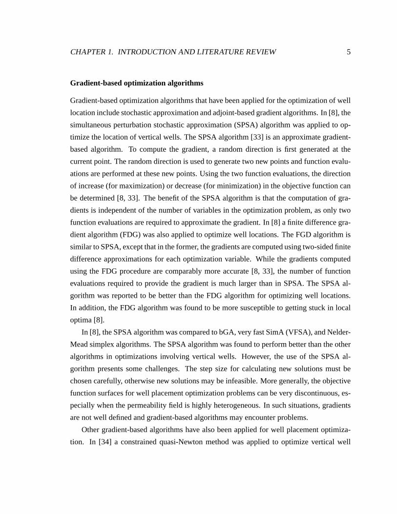
Gradient-based optimization algorithms
Gradient-based optimization algorithms that have been applied for the optimization of well
location include stochastic approximation and adjoint-based gradient algorithms. In [8], the
simultaneous perturbation stochastic approximation (SPSA) algorithm was applied to op-
timize the location of vertical wells. The SPSA algorithm [33] is an approximate gradient-
based algorithm. To compute the gradient, a random direction is first generated at the
current point. The random direction is used to generate two new points and function evalu-
ations are performed at these new points. Using the two function evaluations, the direction
of increase (for maximization) or decrease (for minimization) in the objective function can
be determined [8, 33]. The benefit of the SPSA algorithm is that the computation of gra-
dients is independent of the number of variables in the optimization problem, as only two
function evaluations are required to approximate the gradient. In [8] a finite difference gra-
dient algorithm (FDG) was also applied to optimize well locations. The FGD algorithm is
similar to SPSA, except that in the former, the gradients arecomputed using two-sided finite
difference approximations for each optimization variable. While the gradients computed
using the FDG procedure are comparably more accurate [8, 33], the number of function
evaluations required to provide the gradient is much largerthan in SPSA. The SPSA al-
gorithm was reported to be better than the FDG algorithm for optimizing well locations.
In addition, the FDG algorithm was found to be more susceptible to getting stuck in local
optima [8].
In [8], the SPSA algorithm was compared to bGA, very fast SimA(VFSA), and Nelder-
Mead simplex algorithms. The SPSA algorithm was found to perform better than the other
algorithms in optimizations involving vertical wells. However, the use of the SPSA al-
gorithm presents some challenges. The step size for calculating new solutions must be
chosen carefully, otherwise new solutions may be infeasible. More generally, the objective
function surfaces for well placement optimization problems can be very discontinuous, es-
pecially when the permeability field is highly heterogeneous. In such situations, gradients
are not well defined and gradient-based algorithms may encounter problems.
Other gradient-based algorithms have also been applied forwell placement optimiza-
tion. In [34] a constrained quasi-Newton method was appliedto optimize vertical well
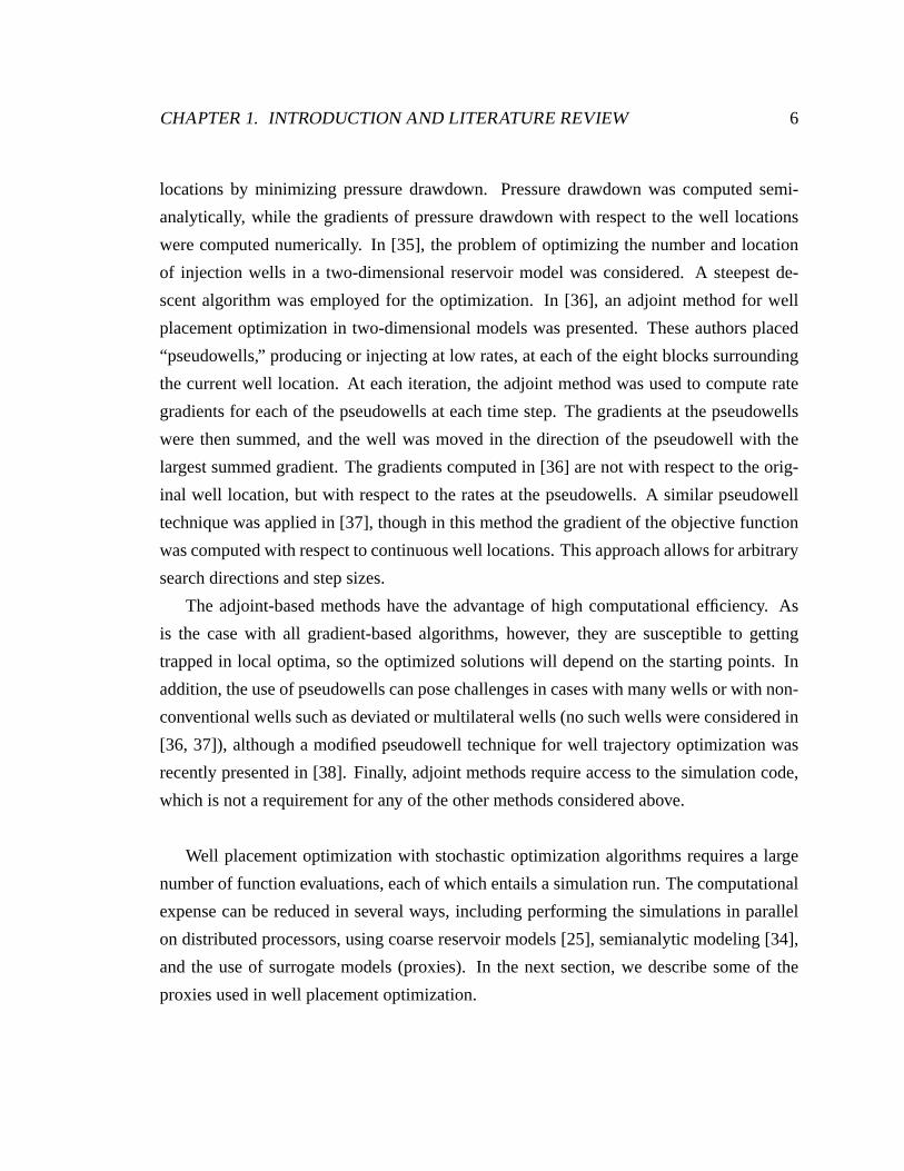
CHAPTER 1. INTRODUCTION AND LITERATURE REVIEW 6
locations by minimizing pressure drawdown. Pressure drawdown was computed semi-
analytically, while the gradients of pressure drawdown with respect to the well locations
were computed numerically. In [35], the problem of optimizing the number and location
of injection wells in a two-dimensional reservoir model wasconsidered. A steepest de-
scent algorithm was employed for the optimization. In [36],an adjoint method for well
placement optimization in two-dimensional models was presented. These authors placed
“pseudowells,” producing or injecting at low rates, at eachof the eight blocks surrounding
the current well location. At each iteration, the adjoint method was used to compute rate
gradients for each of the pseudowells at each time step. The gradients at the pseudowells
were then summed, and the well was moved in the direction of the pseudowell with the
largest summed gradient. The gradients computed in [36] arenot with respect to the orig-
inal well location, but with respect to the rates at the pseudowells. A similar pseudowell
technique was applied in [37], though in this method the gradient of the objective function
was computed with respect to continuous well locations. This approach allows for arbitrary
search directions and step sizes.
The adjoint-based methods have the advantage of high computational efficiency. As
is the case with all gradient-based algorithms, however, they are susceptible to getting
trapped in local optima, so the optimized solutions will depend on the starting points. In
addition, the use of pseudowells can pose challenges in cases with many wells or with non-
conventional wells such as deviated or multilateral wells (no such wells were considered in
[36, 37]), although a modified pseudowell technique for welltrajectory optimization was
recently presented in [38]. Finally, adjoint methods require access to the simulation code,
which is not a requirement for any of the other methods considered above.
Well placement optimization with stochastic optimizationalgorithms requires a large
number of function evaluations, each of which entails a simulation run. The computational
expense can be reduced in several ways, including performing the simulations in parallel
on distributed processors, using coarse reservoir models [25], semianalytic modeling [34],
and the use of surrogate models (proxies). In the next section, we describe some of the
proxies used in well placement optimization.
CHAPTER 1. INTRODUCTION AND LITERATURE REVIEW 7
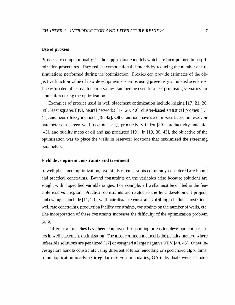
Use of proxies
Proxies are computationally fast but approximate models which are incorporated into opti-
mization procedures. They reduce computational demands byreducing the number of full
simulations performed during the optimization. Proxies can provide estimates of the ob-
jective function value of new development scenarios using previously simulated scenarios.
The estimated objective function values can then be used to select promising scenarios for
simulation during the optimization.
Examples of proxies used in well placement optimization include kriging [17, 21, 26,
39], least squares [39], neural networks [17, 20, 40], cluster-based statistical proxies [13,
41], and neuro-fuzzy methods [19, 42]. Other authors have used proxies based on reservoir
parameters to screen well locations, e.g., productivity index [30], productivity potential
[43], and quality maps of oil and gas produced [19]. In [19, 30, 43], the objective of the
optimization was to place the wells in reservoir locations that maximized the screening
parameters.
Field development constraints and treatment
In well placement optimization, two kinds of constraints commonly considered are bound
and practical constraints. Bound constraints on the variables arise because solutions are
sought within specified variable ranges. For example, all wells must be drilled in the fea-
sible reservoir region. Practical constraints are relatedto the field development project,
and examples include [11, 29]: well-pair distance constraints, drilling schedule constraints,
well rate constraints, production facility constraints, constraints on the number of wells, etc.
The incorporation of these constraints increases the difficulty of the optimization problem
[3, 6].
Different approaches have been employed for handling infeasible development scenar-
ios in well placement optimization. The most common method is the penalty method where
infeasible solutions are penalized [17] or assigned a largenegative NPV [44, 45]. Other in-
vestigators handle constraints using different solution encoding or specialized algorithms.
In an application involving irregular reservoir boundaries, GA individuals were encoded
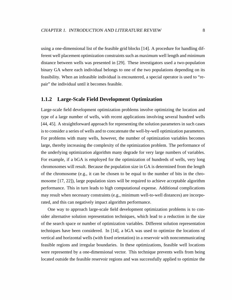
CHAPTER 1. INTRODUCTION AND LITERATURE REVIEW 8
using a one-dimensional list of the feasible grid blocks [14]. A procedure for handling dif-
ferent well placement optimization constraints such as maximum well length and minimum
distance between wells was presented in [29]. These investigators used a two-population
binary GA where each individual belongs to one of the two populations depending on its
feasibility. When an infeasible individual is encountered,a special operator is used to “re-
pair” the individual until it becomes feasible.
1.1.2 Large-Scale Field Development Optimization
Large-scale field development optimization problems involve optimizing the location and
type of a large number of wells, with recent applications involving several hundred wells
[44, 45]. A straightforward approach for representing the solution parameters in such cases
is to consider a series of wells and to concatenate the well-by-well optimization parameters.
For problems with many wells, however, the number of optimization variables becomes
large, thereby increasing the complexity of the optimization problem. The performance of
the underlying optimization algorithm many degrade for very large numbers of variables.
For example, if a bGA is employed for the optimization of hundreds of wells, very long
chromosomes will result. Because the population size in GA isdetermined from the length
of the chromosome (e.g., it can be chosen to be equal to the number of bits in the chro-
mosome [17, 22]), large population sizes will be required toachieve acceptable algorithm
performance. This in turn leads to high computational expense. Additional complications
may result when necessary constraints (e.g., minimum well-to-well distances) are incorpo-
rated, and this can negatively impact algorithm performance.
One way to approach large-scale field development optimization problems is to con-
sider alternative solution representation techniques, which lead to a reduction in the size
of the search space or number of optimization variables. Different solution representation
techniques have been considered. In [14], a bGA was used to optimize the locations of
vertical and horizontal wells (with fixed orientation) in a reservoir with noncommunicating
feasible regions and irregular boundaries. In these optimizations, feasible well locations
were represented by a one-dimensional vector. This technique prevents wells from being
located outside the feasible reservoir regions and was successfully applied to optimize the
CHAPTER 1. INTRODUCTION AND LITERATURE REVIEW 9
location of 33 new wells in a real field application. However,the length of the GA indi-
vidual will increase with the number of wells considered. Itwas shown in [16] that this
approach is not efficient because of major discontinuities in the search.
Another solution representation technique that leads to reduction in the number of vari-
ables is to consider well patterns in the optimization. Kriging and least-square algorithms
were applied in [39] to optimize the location of an inverted five-spot pattern element in a
waterflooding project. The pattern element was representedwith four optimization vari-
ables: the spatial location of the injector and two well spacing parameters. A fixed pattern
approach (FPA) for optimizing wells in reservoirs with irregular boundaries was also used
in [32]. In FPA, wells are optimized in a line drive pattern using two optimization variables
- well spacing and distance to the reservoir boundary. The procedure, which was applied to
a field case, reduced the number of simulations required in the optimization. A robust field
development procedure, described in [45], was applied successfully to giant fields [44, 46].
To reduce the number of optimization variables, three different pattern types were consid-
ered: inverted five-spot, inverted seven-spot, and staggered line drives. These investigators
considered different well types and a specified set of well spacings in their optimizations.
In optimizations using concatenated well-by-well parameters, treatment of well-pair
distance constraints requires specifying user-defined threshold values. These values have
the effect of reducing the search space of solutions considered and may affect the quality of
solutions obtained. In optimizations with well patterns, the optimum pattern type, size, and
orientation for a given application are unknown. Previous applications with well patterns
consider a single pattern type [32, 39], or a set of well patterns with fixed well spacings
[45]. In this thesis, we introduce a new well pattern optimization procedure that generalizes
previous techiniques. We will show that this approach is well suited for optimizing large-
scale field development.
1.1.3 Particle Swarm Optimization (PSO) Algorithm
The particle swarm optimization (PSO) algorithm [47, 48, 49, 50] is a relatively new al-
gorithm for global optimization. The algorithm mimics the social interactions exhibited in
CHAPTER 1. INTRODUCTION AND LITERATURE REVIEW 10
animal groups, e.g., in fish swarms and in bird flocks. Like theGA, PSO is a population-
based algorithm. PSO solutions are referred to as particlesrather than individuals as in GA.
The collection of particles in a given iteration is called the swarm. The position of each
particle is adjusted according to its fitness and position relative to the other particles in the
swarm.
The GA and PSO algorithms share some similarities. Both algorithms have operators
to create new solutions from existing solutions. Both also include random components to
prevent solutions from being trapped in local optima. The algorithms differ, however, in
the number and type of operators used to create and improve solutions during the optimiza-
tion. GA has three main operators: selection, crossover, and mutation. There are many
strategies for applying these operators [51, 52], and the best option will depend on the spe-
cific optimization problem [7, 22]. The basic PSO algorithm,by constrast, has one main
operator, the “velocity” equation, which consists of several components and moves the par-
ticle through the search space with a velocity (though, in PSO, each particle also carries a
memory). The velocity provides the search directions for each particle, and is updated in
each iteration of the algorithm. The GA and PSO algorithms also differ in the number of
vectors associated with each individual or particle. In GA,there is one solution vector for
each individual. However, for PSO, there are three vectors associated with each particle:
current position, velocity, and previous best position.
The PSO algorithm uses a cooperative search strategy for optimization where particles
interact with each other. This interaction is achieved using neighborhoods, where a particle
can only interact with other particles in its neighborhood [2, 3, 53]. Depending on the
number of neighborhoods used, the global best (gbest) and local best (lbest) PSO variants
are obtained [3]. In gbest PSO, a single neighborhood containing all the particles is used.
For the lbest PSO, more than one neighborhood is employed in the optimization, and each
particle may belong to multiple neighborhoods.
The computation of particle velocities at each iteration uses the locations of the best
particles found so far. Particle velocities are computed similarly for the gbest and lbest
PSO variants, except that in gbest PSO, the best particle in the entire swarm is used, while
in the lbest PSO, the best particle in a particle’s neighborhood is used. The choice of
neighborhood topology also affects the PSO algorithm performance and different types

CHAPTER 1. INTRODUCTION AND LITERATURE REVIEW 11
of neighborhood topologies (e.g., random, ring) have been developed [2, 3, 54, 55]. Faster
convergence is observed for gbest PSO, but there is a higher susceptibility of getting trapped
in local optima. On the other hand, the lbest PSO is slower, but can provide robust results
especially in problems with many local optima [3, 53].
The PSO algorithm has been applied successfully in many different application areas
such as training neural networks [47, 48, 56], dynamic economic dispatch problems [57],
pole shape optimization [58], water reservoir operations and planning [59], placement of
sensors for civil structures [60], geophysical inverse problems [61] and flow shop schedul-
ing problems [62]. Although the PSO algorithm does not appear to have been applied pre-
viously within the context of oil reservoir simulation, it has been used for related subsurface
flow applications. Specifically, in [63] PSO was applied to a contaminated groundwater re-
mediation problem using analytical element models. The investigators minimized the cost
of remediation by optimizing the number, location, and rates of (vertical) extraction and
injection wells. Several algorithms were applied, including continuous GA, simulated an-
nealing, and Fletcher-Reeves conjugate gradient. The best results were obtained using the
PSO algorithm. The authors also compared the effectivenessof GA and PSO algorithms
for the elimination of wells when the number of wells required was overspecified. The PSO
algorithm was also found to be more effective for this application. These findings provide a
key motivation for our work on applying the PSO algorithm to well placement optimization
problems. Furthermore, the PSO algorithm has been found to provide better results, and in
general to require fewer function evaluations, than GA [61,62, 64] and SimA [61] algo-
rithms for applications involving scheduling, geologicalinversion and computer hardware
design.
Like other stochastic optimization algorithms, the performance of PSO depends on the
values assigned to the parameters in the algorithm. We now discuss previous work related
to choosing PSO parameter values.
CHAPTER 1. INTRODUCTION AND LITERATURE REVIEW 12
PSO parameter selection
The PSO algorithm has several parameters which must be specified before performing an
optimization run. These include population size, the maximum number of iterations, and
the weights of the inertia (ω), cognitive (c1), and social (c2) components of the velocity
equation [3]. These weights affect the trajectories of the particles. If a local best PSO
variant is used, a neighborhood topology must also be specified. The swarm size affects
the search ability of the PSO algorithm and it is chosen basedon the size of the search space
and problem difficulty [53]. Population sizes in the range of20-40 were recommended in
[2, 53].
Several authors have proposed specific PSO parameter valuesor techniques for obtain-
ing appropriate parameter values. Values ofω = 1, c1 = c2 = 2.0 were used in [47, 48].
These were heuristic values and have since been found to violate PSO convergence re-
quirements [3, 53]. It has been shown that particle trajectories can be converging, cyclic or
diverging [3]. Modifications have been introduced to curb particle divergence issues, e.g.,
use of velocity clamping (or restriction) and use of inertial weights other than unity, for
exampleω = 0.729 in [65]. These modifications lead to better convergence characteristics
of the PSO algorithm.
Others authors studied the stability and convergence of thePSO particle trajectories
(see for example [50, 58, 66, 67, 68]) in order to understand particle dynamics and to
choose optimal PSO parameters. These studies provided detailed mathematical analyses
describing the relationships between particle trajectoryand the values ofω, c1, andc2. The
different parameter regions (i.e., values ofω, c1, andc2) where a particle’s trajectory would
converge were shown in [50]. In [66], so-called parameter clouds were proposed where
the values ofω, c1, andc2 were selected based on the results of exhaustive sampling of
ω, c1, andc2 in optimizations involving mathematical functions, e.g.,the Rosenbrock and
Griewank functions. The first step in the cloud method is to select several parameter points
(combinations ofω, c1 and c2) from the regions that resulted in low objective function
values (for minimization). Then, the selected parameters were used in other optimization
problems. A constriction factor, which damps the computed particle velocity and ensures
CHAPTER 1. INTRODUCTION AND LITERATURE REVIEW 13
that the swarm converges, was introduced in [67]. DifferentPSO variants with parameter
values determined from analysis of particle trajectories were developed in [68].
The work [61, 66, 67, 68] on particle swarm stability and convergence often involves
some simplifications [3]. For example, these studies involve a single particle, and the
effect of particle-particle interactions are not considered. Another method for determining
optimal PSO parameters is to actually optimize the parameter values during optimization.
This method is described in the next section.
1.1.4 Metaoptimization for Parameter Determination
The parameters in the PSO algorithm can be directly optimized for a given optimization
problem [2, 69, 70, 71]. This method, referred to as metaoptimization [69, 70, 71], elimi-
nates the need to specify parameter values for a given problem (the cloud method described
in the previous section also eliminates this need).
Metaoptimization involves the use of two optimization algorithms. Within the context
of PSO, the first algorithm optimizes the PSO parameters, while the second one optimizes
the specific optimization problem using the PSO parameters obtained from the first algo-
rithm. In practice, any optimization algorithm can be used for optimizing the PSO param-
eters. PSO is commonly employed for this purpose [2, 69, 70],although a continuous GA
was used in [71].
We focus on applications that use PSO for optimizing the parameter values. The first
and second PSO algorithms are referred to as the “superswarmPSO” and “subswarm PSO”
respectively [69]. Each superswarm PSO particle corresponds to a point in the search space
of PSO parameters (e.g.,ω, c1, c2). The fitness of a superswarm particle is computed by
performing several subswarm optimizations using the parameters from the superswarm
particle. The subswarm optimizations are performed on either the target problem or one
or more representative optimization problems, in our case,a well placement optimization.
The fitness functions are defined differently for the subswarm and superswarm and depend
on the objective function in the subswarm. In the subswarm, the objective is to minimize
some error (if the global optimum is known) or maximize some objective function, e.g.,
CHAPTER 1. INTRODUCTION AND LITERATURE REVIEW 14
NPV in well placement optimization problems. In the superswarm optimizations, the ob-
jective is to minimize average error, or maximize the average objective function value from
several subswarm optimization runs. Multiple subswarm optimization runs are performed
for each superswarm particle because of the stochastic nature of the PSO algorithm. The
above-mentioned metaoptimization applications (except [2]) used a gbest PSO with a sin-
gle neighborhood, while [2] considered two types of neighborhood topologies.
The metaoptimization procedure has been demonstrated to provide better results com-
pared to standard PSO with unoptimized parameter values [69, 70, 71]. However, this
method is computationally intensive due to the large numberof function evaluations re-
quired. A large number of function evaluations is needed because the actual optimization
problem is solved many times (in subswarm optimization runs) using different PSO param-
eters. As a result, many metaoptimization studies [2, 70, 71] have used computationally
inexpensive mathematical test functions, e.g., Rosenbrock, Rastrigin and Sphere functions
[2, 3], for the subswarm optimizations.
The metaoptimization procedure can be used in two ways. First, it can be applied
to determine the best PSO parameters for a given set of small,benchmark optimization
problems, where the objective function surfaces are known through exhaustive sampling.
Then, the optimized PSO parameters are used to solve realistic problems in the hope that the
PSO parameters are optimal (or at least reasonable) for these problems. In [2], several PSO
parameters including population size, number of particlesinformed, topology type (random
and circular),ω, c1, andc2, were optimized over several mathematical test functions.After
the metaoptimizations, the number of particles informed (for most functions) was found to
be 3. In all test functions considered, a variable random neighborhood topology was found
to be better than a fixed circular topology.
Metaoptimization can also be applied directly to each new optimization problem. Such
an application may be preferable because the best parametersettings will in general de-
pend on the specific problem considered. In [69], a metaoptimization procedure was used
for training neural networks, where PSO parameters, in addition to the number of hidden
layers in the network, were optimized for the subswarm. These researchers reduced the
computational expense by using a smaller number of particles and fewer iterations in the
CHAPTER 1. INTRODUCTION AND LITERATURE REVIEW 15
superswarm PSO. They also performed several PSO optimizations using the optimized pa-
rameters for similar optimization problems. The results were compared to those obtained
using standard PSO (with parameters from the literature). The PSO with the optimized
parameters was found to provide the best results. Specifically, [69] reported that the PSO
with optimized parameters produced more robust results andconverged faster for the train-
ing of neural networks. Motivated by these findings, we will explore the use of a metaopti-
mization procedure for determining PSO parameter values for well placement optimization
problems.
1.2 Scope of Work
Optimizing the placement of new wells in a field development project is essential in order
to maximize project profitability. This dissertation focuses on the development of efficient
optimization algorithms and procedures for these types of optimizations. We applied the
PSO algorithm to different optimization problems. We also devised a new procedure for
large-scale field development optimization. In this methodology, the number of optimiza-
tion variables does not increase with well count. Finally, we studied the use of metaopti-
mization techniques to improve the performance of the PSO algorithm for well placement
optimization.
This objectives of this research were:
• to evaluate and apply the PSO algorithm for well placement optimization problems.
We considered several optimization problems and compared PSO optimization re-
sults to those obtained using bGA. The examples considered involved different num-
bers of wells, well types (producer and injector, vertical and nonconventional), num-
ber of realizations, and size of the search space.
• to develop and apply new approaches for large-scale field development optimization
involving many wells. We developed a new well pattern optimization (WPO) al-
gorithm which contains two optimization phases. In the firstphase, optimizations
CHAPTER 1. INTRODUCTION AND LITERATURE REVIEW 16
were performed using a new (generic) well pattern description. In the (optional) sec-
ond phase, phase 1 solutions were improved further using well-by-well perturbation.
In both phases, we used the PSO algorithm for the underlying optimizations. We
considered different optimization problems including a case with multiple reservoir
models and a reservoir with an irregular boundary.
• to improve the performance of the PSO algorithm for well placement optimization
using metaoptimization. For this study, we applied PSO metaoptimization techniques
to a variety of well placement optimization problems.
1.3 Dissertation Outline
This dissertation is organized as follows. In Chapter 2, we discuss the application of
the PSO algorithm to several well placement optimization problems. First, we describe
the PSO algorithm in detail, presenting different variantsof the algorithm, neighborhood
topologies, and treatment of infeasible particles. We thenconsider several optimization
problems of varying complexity in terms of the size of the search space, the dimension
and size of the reservoir, and the number and type of wells considered. We compare PSO
optimization results to those obtained with a binary GA implemenation. For all examples,
we performed multiple optimization runs because of the stochastic nature of the GA and
PSO algorithms.
The PSO algorithm performed very well for all of the optimization problems consid-
ered. In one example, we assessed the sensitivity of PSO and GA results to varying swarm
(population) sizes. For small swarm/population sizes, thePSO algorithm achieved better
results than bGA. The performance of both algorithms was about the same for large popu-
lation sizes. The senstivity results indicated that PSO finds similar or better solutions than
bGA using fewer function evaluations. These findings are in agreement with those ob-
served by [61, 62, 64]. Other examples were also considered including optimizing the well
type and location of 20 vertical wells, optimizing the location of four deviated producers,
and optimizing the location of two dual-lateral wells. In these examples, PSO achieved
better results (on average) than bGA. The work presented in Chapter 2 has been published

CHAPTER 1. INTRODUCTION AND LITERATURE REVIEW 17
in Computational Geosciences[72].
Chapter 2 describes the application of the PSO algorithm to a problem involving up
to 20 vertical wells, in which the well-by-well optimization parameters are simply con-
catenated. Using this approach in large-scale field development projects would result in a
great number number of variables and a very large search space. In Chapter 3, we intro-
duce a new procedure, called the well pattern optimization (WPO) algorithm, which can
be used for optimization problems involving a large number of wells. WPO consists of
a new well pattern description (WPD), followed by an optionalwell-by-well perturbation
(WWP), with both procedures incorporated into a core PSO methodology. WPD repre-
sents solutions at the level of well patterns rather than individual wells, which can lead to
a significant reduction in the number of optimization variables. Using WPD, the number
of optimization variables is independent of the number of wells considered. In WPD, each
potential solution consists of three elements: parametersthat define the basic well pattern,
parameters that define so-called well pattern operators, and the sequence of application of
these operators. The well pattern operators define pattern transformations that vary the
size, shape and orientation of the well patterns consideredin the optimization. The opti-
mum number of wells required, in addition to the producer-injector ratio, is obtained from
the optimization. Optimized solutions based on WPD are always repeated patterns; i.e., the
method does not lead to irregular well placements. The subsequent use of WWP allows
(limited) local shifting of all wells in the model, which enables the optimization to account
for local variations in reservoir properties.
The WPO optimization procedure introduced here differs fromthe work of [45] in sev-
eral respects. We used a different technique to represent potential field development scenar-
ios, and our algorithm considers very general well patterns. This was accomplished through
use of pattern transformation operations, which allow patterns to be rotated, stretched or
sheared to an optimal degree. This can be important, for example, in situations where there
are preferential flow directions in the field. In addition to standard patterns, the algorithm
accepts user-defined patterns. WPD also eliminates the need for well-to-well distance con-
straints in the optimization. This is useful as highly constrained optimization problems are
generally more difficult to solve than less constrained problems [3, 6]. Finally, the use of
CHAPTER 1. INTRODUCTION AND LITERATURE REVIEW 18
WWP enables the local adjustment of well locations.
The WPD and WWP procedures were applied to different well placement optimization
problems. In these examples, we performed multiple optimizations using the WPO pro-
cedure to gauge the degree of variability in the runs. In one problem, we compared WPD
optimizations using one and four well pattern operators. The results show that better results
were obtained using four well pattern operators. We performed both WPD and WWP op-
timizations for two examples, one involving five realizations of a reservoir model, and the
other a reservoir with an irregular boundary. These optimizations demonstrated our ability
to optimize large-scale field development. In the examples that use WWP optimizations,
WWP was shown to improve the objective function value in each optimization run. Specif-
ically, average improvements in NPV of 22% and 34% over the best WPD solutions were
obtained.
The main benefits of the WPO procedure are that the optimum number of wells is de-
termined during the optimization and that well-pair distance constraints do not need to be
considered. Part of the work presented in Chapter 3 has been published in [73].
In the work described in Chapters 2 and 3, we applied PSO default parameter values
suggested in the literature. These values were obtained from an analysis of particle trajec-
tories and numerical experiments with mathematical functions [68]. In Chapter 4, we show
the application of the metaoptimization procedure to optimize PSO parameters.
We first applied the metaoptimization procedure for four benchmark well placement op-
timization problems. Because of the very large number of function evaluations required by
the metaoptimization procedure, we computed the full objective function surface exhaus-
tively for each problem. This allowed inexpensive repetitions of optimization runs because
we only needed to look up the NPV values. We demonstrated thatthe metaoptimization
procedure provides better results than those obtained using PSO with unoptimized param-
eters. These results are consistent with those found in other PSO metaoptimization studies
[68, 69].
Next, we used the metatoptimization procedure for realistic well placement optimiza-
tion problems. We considered two optimization problems. Inthe first, we optimized the
type and location of 15 wells using the well-by-well concatenation approach. In the second
CHAPTER 1. INTRODUCTION AND LITERATURE REVIEW 19
problem, we performed WPO optimizations. The metaoptimization results were shown to
give better results than those using default parameters or parameters from the benchmark
problems.
In Chapter 5, we present conclusions and recommendations forfuture research on the
development of robust and efficient procedures for well placement optimization.
Chapter 2
Use of PSO for Well Placement
Optimization
In this chapter, we describe the details of the PSO algorithmused in this work. Well
placement optimization problems of varying complexity were considered. These problems
included optimizing the location of a single producer over ten reservoir models, optimizing
the location and type of 20 vertical wells, optimizing the location of four deviated pro-
ducers, and optimizing the location of two dual-lateral producers. In each problem, we
performed multiple optimizations using the PSO algorithm and compared results to those
obtained using bGA. These results demonstrate the superiorperformance of PSO for the
cases considered.
2.1 Particle Swarm Optimization (PSO) Algorithm
The PSO algorithm is a population-based stochastic optimization procedure developed by
[47, 48]. The algorithm mimics the social behaviors exhibited by swarms of animals. In the
PSO algorithm, a point in the search space (i.e., a possible solution) is called a particle. The
collection of particles in a given iteration is referred to as the swarm. The terms ‘particle’
and ‘swarm’ are analogous to ‘individual’ and ‘population’used in evolutionary algorithms
such as GAs. We will use these terms interchangeably in this chapter.
At each iteration, each particle in the swarm moves to a new position in the search
20
CHAPTER 2. USE OF PSO FOR WELL PLACEMENT OPTIMIZATION 21
space. We denotex as a potential solution in the search space of ad-dimensional optimiza-
tion problem,xi(k) = {xi,1(k), . . . , xi,d(k)} as the position of theith particle in iteration
k, xpbesti (k) as the previous best solution found by theith particle up to iterationk, and
xnbesti (k) as the position of the best particle in the neighborhood of particle xi up to itera-
tionk. We will discuss neighborhood topologies in detail in Section 2.1.1. One option is for
the neighborhood to include the full swarm of particles, in which case,xnbesti (k) = x
g(k),
wherexg(k) is the global best particle position.
The new position of particlei in iterationk + 1, xi(k + 1), is computed by adding a
velocity,vi(k + 1), to the current positionxi(k) [47, 48, 65]:
xi(k + 1) = xi(k) + vi(k + 1) · ∆t, (2.1)
wherevi(k+1) = {vi,1(k+1), . . . , vi,d(k+1)} is the velocity of particlei at iterationk+1,
and∆t is a ‘time’ increment. Here, consistent with standard PSO implementations, we set
∆t = 1. It should be noted, however, that recent work has demonstrated improved results
using variable∆t [50, 49], so this might be worthwhile to consider in future investigations.
The elements of the velocity vector are computed as [3, 65]:
vi(k + 1) = ω · vi(k)
+ c1 · D1(k) · (xpbesti (k) − xi(k))
+ c2 · D2(k) · (xnbesti (k) − xi(k)),
(2.2)
whereω, c1 andc2 are weights;D1(k) andD2(k) are diagonal matrices whose diagonal
components are uniformly distributed random variables in the range [0, 1]; andj, j ∈
{1, 2, . . . , d}, refers to thejth optimization variable. In the optimizations performed in this
chapter, we setω = 0.721 and c1 = c2 = 1.193. These values were determined from
numerical experiments performed by [68]. We note that it is possible to optimize these
parameters as part of the overall procedure. A metaoptimization procedure that optimizes
the PSO parameters during optimization will be described inChapter 4.
The velocity equation (Eq. 2.2) has three components, referred to as the inertia (term
involving ω), cognitive (term involvingc1), and social (term involvingc2) components
respectively [3]. The inertia component provides a degree of continuity in particle velocity
CHAPTER 2. USE OF PSO FOR WELL PLACEMENT OPTIMIZATION 22
from one iteration to the next, while the cognitive component causes the particle to move
towards its own previous best position. The social component, by contrast, moves the
particle toward the best particle in its neighborhood. These three components perform
different roles in the optimization. The inertia componentenables a broad exploration of
the search space, while the cognitive and social componentsnarrow the search toward the
promising solutions found up to the current iteration.
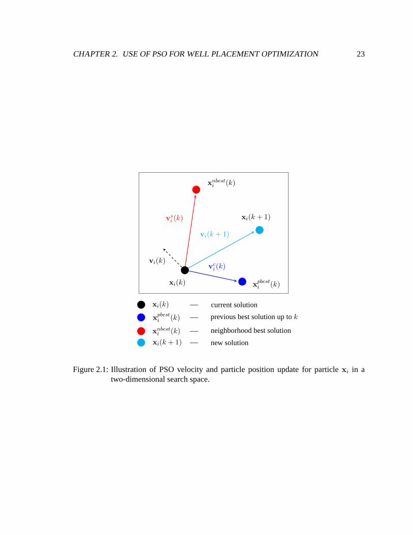
Figure 2.1 shows the velocity computation and solution update in iterationk + 1, for a
particle in a two-dimensional search space. Herevi(k) is the particle’s previous velocity,
whilevci (k) is the velocity (cognitive) from the current position (xi(k)) to the particle’s pre-
vious best position (xpbesti (k)), andv
si (k) is the velocity (social) from the current position
to the current neighborhood best position (xnbesti (k)). The velocity vectorsvi(k), v
si (k),
andvci (k) are used to computevi(k + 1) according to Eq. 2.2. The new particle velocity,
vi(k + 1), is added to the current position to obtain the new position vector,xi(k + 1), as
shown in Eq. 2.1.
2.1.1 PSO Neighborhood Topology
Particle topologies or neighborhoods refer to the groupingof particles into subgroups. A
particle can communicate and exchange information about the search space only with other
particles in its neighborhood [2]. The performance of the PSO algorithm depends to some
extent on the neighborhood topology, as discussed below. A particle j is in the neighbor-
hood of particlei if there is a ‘link’ from particlei to j. This means that particlej informs
particlei about its position in the search space. Particlej is called the informing particle
(informant), while particlei is called the informed particle [2]. Each particle is a member
of its neighborhood, i.e., each particle informs itself. The neighborhood size refers to the
number of particles in the neighborhood.
The neighborhood topology is defined by a so-called adjacency matrix mij, where the
rows correspond to informing particles and the columns correspond to the informed parti-
cles. In general, the matrix is nonsymmetric and contains zeros and ones as entries, with an
entry of one indicating that particlei is contained in the neighborhood of particlej (particle
i informs particlej). The matrix always has ones on the diagonal because each particle is
CHAPTER 2. USE OF PSO FOR WELL PLACEMENT OPTIMIZATION 23
xi(k)
xnbesti (k)
xpbesti (k)
xi(k + 1)vsi (k)
vci (k)
vi(k)
vi(k + 1)
xi(k) — current solution
xpbesti (k) — previous best solution up tok
xnbesti (k) — neighborhood best solution
xi(k + 1) — new solution
Figure 2.1: Illustration of PSO velocity and particle position update for particlexi in atwo-dimensional search space.
CHAPTER 2. USE OF PSO FOR WELL PLACEMENT OPTIMIZATION 24
contained in its own neighborhood. Using the adjacency matrix, it is possible to define
different types of neighborhood topologies.
In all topologies considered in this work, the locations of the particles in the search
space do not affect the neighborhood, as only the particles’indices are required to define
the topologies. Here, particle index refers to the positionof the particle in the array of
particles.
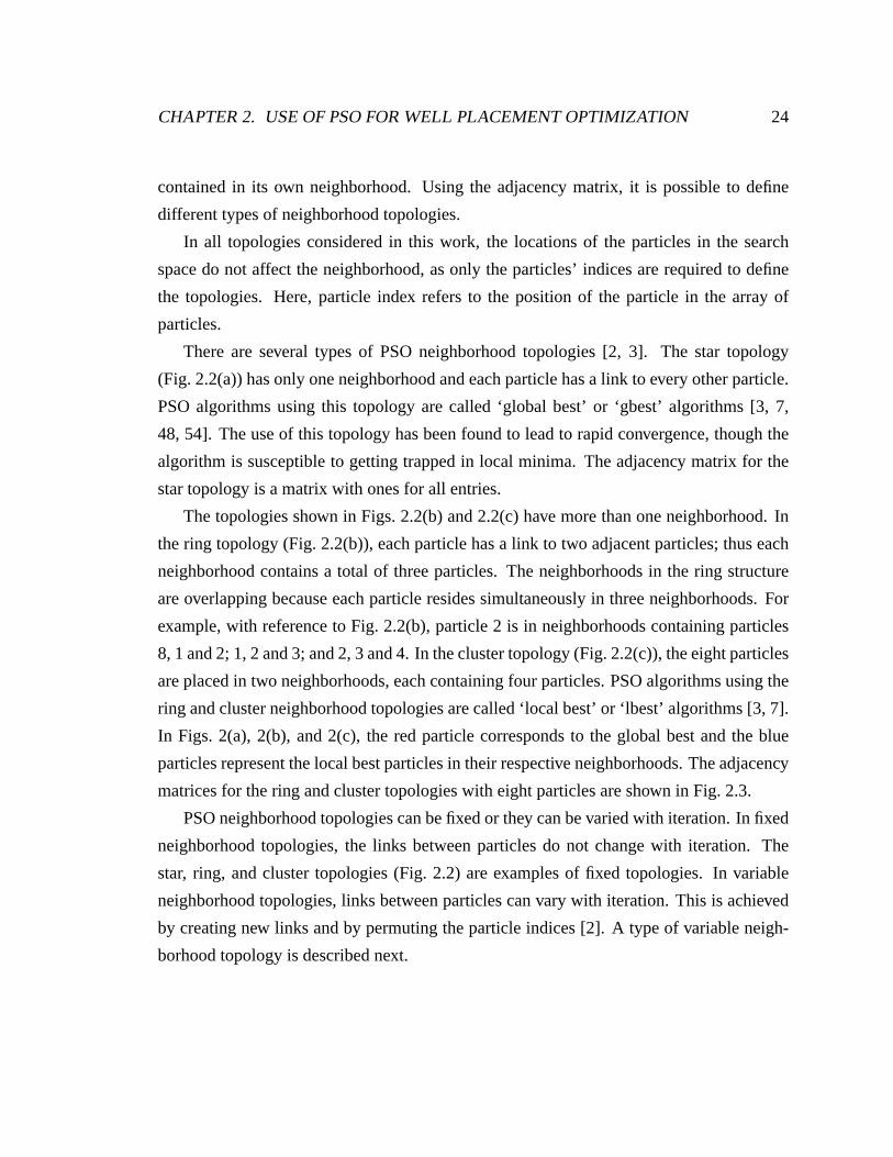
There are several types of PSO neighborhood topologies [2, 3]. The star topology
(Fig. 2.2(a)) has only one neighborhood and each particle has a link to every other particle.
PSO algorithms using this topology are called ‘global best’or ‘gbest’ algorithms [3, 7,
48, 54]. The use of this topology has been found to lead to rapid convergence, though the
algorithm is susceptible to getting trapped in local minima. The adjacency matrix for the
star topology is a matrix with ones for all entries.
The topologies shown in Figs. 2.2(b) and 2.2(c) have more than one neighborhood. In
the ring topology (Fig. 2.2(b)), each particle has a link to two adjacent particles; thus each
neighborhood contains a total of three particles. The neighborhoods in the ring structure
are overlapping because each particle resides simultaneously in three neighborhoods. For
example, with reference to Fig. 2.2(b), particle 2 is in neighborhoods containing particles
8, 1 and 2; 1, 2 and 3; and 2, 3 and 4. In the cluster topology (Fig. 2.2(c)), the eight particles
are placed in two neighborhoods, each containing four particles. PSO algorithms using the
ring and cluster neighborhood topologies are called ‘localbest’ or ‘lbest’ algorithms [3, 7].
In Figs. 2(a), 2(b), and 2(c), the red particle corresponds to the global best and the blue
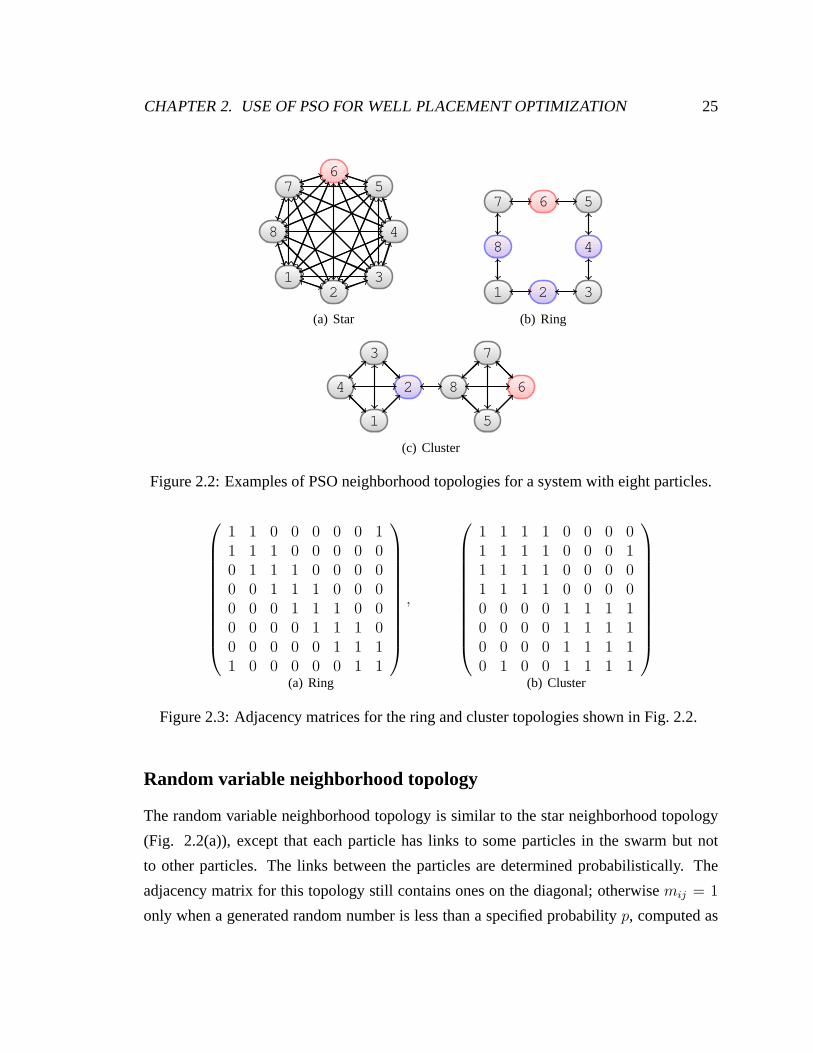
particles represent the local best particles in their respective neighborhoods. The adjacency
matrices for the ring and cluster topologies with eight particles are shown in Fig. 2.3.
PSO neighborhood topologies can be fixed or they can be variedwith iteration. In fixed
neighborhood topologies, the links between particles do not change with iteration. The
star, ring, and cluster topologies (Fig. 2.2) are examples of fixed topologies. In variable
neighborhood topologies, links between particles can varywith iteration. This is achieved
by creating new links and by permuting the particle indices [2]. A type of variable neigh-
borhood topology is described next.
CHAPTER 2. USE OF PSO FOR WELL PLACEMENT OPTIMIZATION 25
12
3
4
56
7
8
(a) Star
1 2 3
4
567
8
(b) Ring
1
2
3
4
5
6
7
8
(c) Cluster
Figure 2.2: Examples of PSO neighborhood topologies for a system with eight particles.
1 1 0 0 0 0 0 11 1 1 0 0 0 0 00 1 1 1 0 0 0 00 0 1 1 1 0 0 00 0 0 1 1 1 0 00 0 0 0 1 1 1 00 0 0 0 0 1 1 11 0 0 0 0 0 1 1
,
(a) Ring
1 1 1 1 0 0 0 01 1 1 1 0 0 0 11 1 1 1 0 0 0 01 1 1 1 0 0 0 00 0 0 0 1 1 1 10 0 0 0 1 1 1 10 0 0 0 1 1 1 10 1 0 0 1 1 1 1
(b) Cluster
Figure 2.3: Adjacency matrices for the ring and cluster topologies shown in Fig. 2.2.
Random variable neighborhood topology
The random variable neighborhood topology is similar to thestar neighborhood topology
(Fig. 2.2(a)), except that each particle has links to some particles in the swarm but not
to other particles. The links between the particles are determined probabilistically. The
adjacency matrix for this topology still contains ones on the diagonal; otherwisemij = 1
only when a generated random number is less than a specified probability p, computed as
CHAPTER 2. USE OF PSO FOR WELL PLACEMENT OPTIMIZATION 26
5 10 15 20 25 30 35 400
2
4
6
8
10
Particle index
Num
ber
of p
artic
les
info
rmed
(a) number of informants
5 10 15 20 25 30 35 400
2
4
6
8
10
Particle index
Siz
e of
eac
h ne
ighb
orho
od
(b) neighborhood size
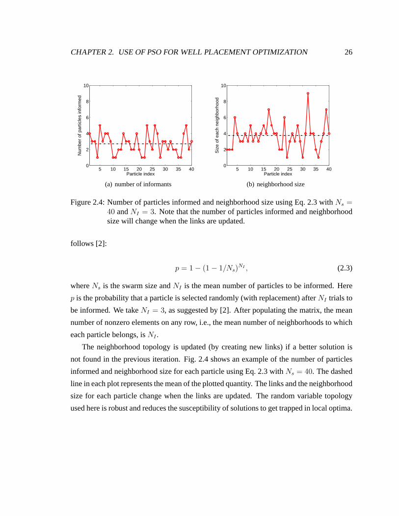
Figure 2.4: Number of particles informed and neighborhood size using Eq. 2.3 withNs =40 andNI = 3. Note that the number of particles informed and neighborhoodsize will change when the links are updated.
follows [2]:
p = 1 − (1 − 1/Ns)NI , (2.3)
whereNs is the swarm size andNI is the mean number of particles to be informed. Here
p is the probability that a particle is selected randomly (with replacement) afterNI trials to
be informed. We takeNI = 3, as suggested by [2]. After populating the matrix, the mean
number of nonzero elements on any row, i.e., the mean number of neighborhoods to which
each particle belongs, isNI .
The neighborhood topology is updated (by creating new links) if a better solution is
not found in the previous iteration. Fig. 2.4 shows an example of the number of particles
informed and neighborhood size for each particle using Eq. 2.3 with Ns = 40. The dashed
line in each plot represents the mean of the plotted quantity. The links and the neighborhood
size for each particle change when the links are updated. Therandom variable topology
used here is robust and reduces the susceptibility of solutions to get trapped in local optima.
CHAPTER 2. USE OF PSO FOR WELL PLACEMENT OPTIMIZATION 27
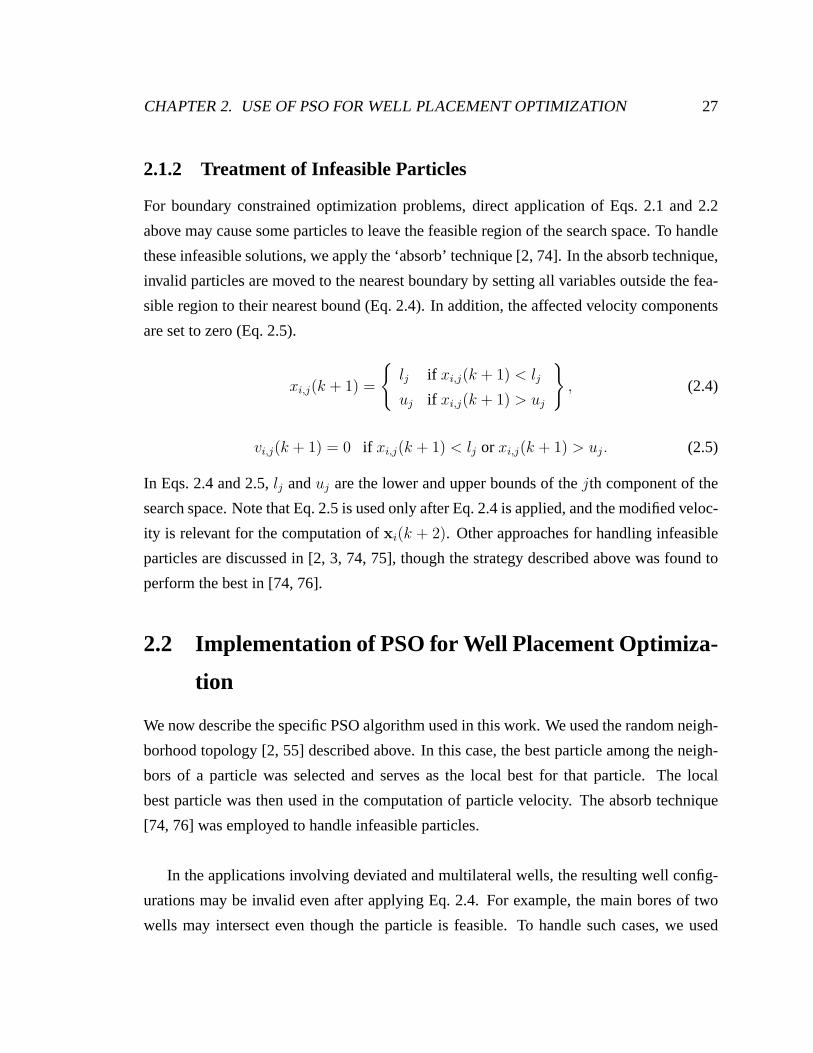
2.1.2 Treatment of Infeasible Particles
For boundary constrained optimization problems, direct application of Eqs. 2.1 and 2.2
above may cause some particles to leave the feasible region of the search space. To handle
these infeasible solutions, we apply the ‘absorb’ technique [2, 74]. In the absorb technique,
invalid particles are moved to the nearest boundary by setting all variables outside the fea-
sible region to their nearest bound (Eq. 2.4). In addition, the affected velocity components
are set to zero (Eq. 2.5).
xi,j(k + 1) =
{
lj if xi,j(k + 1) < lj
uj if xi,j(k + 1) > uj
}
, (2.4)
vi,j(k + 1) = 0 if xi,j(k + 1) < lj or xi,j(k + 1) > uj. (2.5)
In Eqs. 2.4 and 2.5,lj anduj are the lower and upper bounds of thejth component of the
search space. Note that Eq. 2.5 is used only after Eq. 2.4 is applied, and the modified veloc-
ity is relevant for the computation ofxi(k + 2). Other approaches for handling infeasible
particles are discussed in [2, 3, 74, 75], though the strategy described above was found to
perform the best in [74, 76].
2.2 Implementation of PSO for Well Placement Optimiza-
tion
We now describe the specific PSO algorithm used in this work. We used the random neigh-
borhood topology [2, 55] described above. In this case, the best particle among the neigh-
bors of a particle was selected and serves as the local best for that particle. The local
best particle was then used in the computation of particle velocity. The absorb technique
[74, 76] was employed to handle infeasible particles.
In the applications involving deviated and multilateral wells, the resulting well config-
urations may be invalid even after applying Eq. 2.4. For example, the main bores of two
wells may intersect even though the particle is feasible. Tohandle such cases, we used
CHAPTER 2. USE OF PSO FOR WELL PLACEMENT OPTIMIZATION 28
a penalty method where we assigned a negative objective function value to particles that
result in invalid well configurations. This prevents these particles from being selected as
the best particle in their neighborhoods. Other infeasibleparticle treatment techniques are
discussed in [3].
2.2.1 PSO Algorithm Steps
Our implementation of PSO was for parallel computation (allresults presented in this sec-
tion used a cluster of 50 processors). Algorithm 1 presents the steps in the PSO algorithm
for a maximization problem. Step 1 initializes the values ofω, c1, c2, Ns (swarm size size)
andK (number of iterations). The values ofω, c1 and c2 are taken from [68]. Step 3
initializes each component of the particle position,xi,j(k), with random elements drawn
from a uniform distributionU , ∀ j ∈ {1, . . . , D}, ∀ i ∈ {1, . . . , Ns}. Step 4 initializes
each component of the velocities,vi,j(k), to zero. Step 5 computes the objective function
for all particles. In our application, the objective function was evaluated in all cases by
performing a reservoir simulation run (surrogate models were not applied in this work).
Step 6 updates the previous best position for each particle.The particle indices (posi-
tions of particles in the array of particles) are permuted instep 9 (this is not required if the
random variable topology is used), and the neighborhoods for each particle are generated
in step 10. Note that steps 9 and 10 are only performed if the objective function does not
improve in the previous iteration. Step 14 determines the best particle in the neighborhood
of particle i. New particle velocities,vi(k + 1), are computed in step 15. Steps 17-21
update all components of the position of particlei. In step 19, infeasible components of
the position and the corresponding velocity components aremodified using Eqs. 2.4 and
2.5. Step 22 evaluates the objective functionf(xi(k + 1)) based on the new particle po-
sition. The function evaluations in step 22 are carried out in parallel. Steps 25-32 update
the previous best positions for each particle,xpbesti (k), if the new objective function value,
f(xi(k + 1)), is better than that at the previous best position,f(xpbesti (k)). The algorithm
terminates when a maximum number of iterations is reached.
The algorithm described above is a ‘synchronous’ PSO algorithm [2, 3, 76], in which
the previous best particle position for each particle is updated after computing the objective
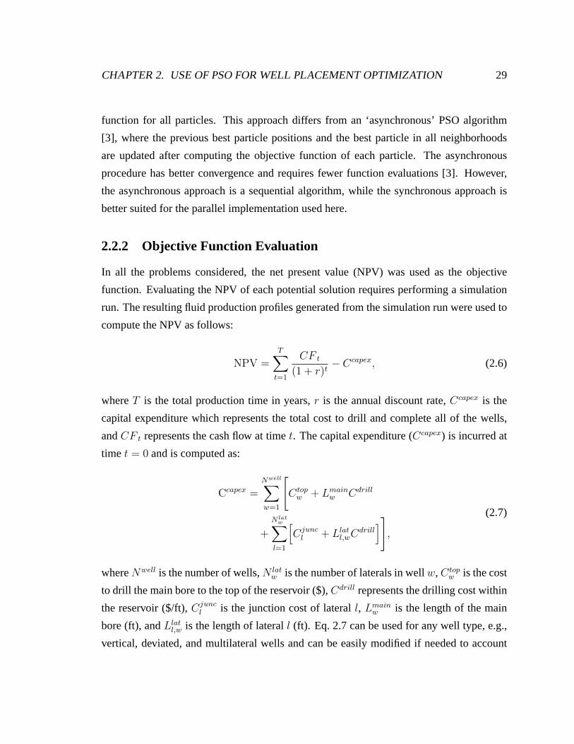
CHAPTER 2. USE OF PSO FOR WELL PLACEMENT OPTIMIZATION 29
function for all particles. This approach differs from an ‘asynchronous’ PSO algorithm
[3], where the previous best particle positions and the bestparticle in all neighborhoods
are updated after computing the objective function of each particle. The asynchronous
procedure has better convergence and requires fewer function evaluations [3]. However,
the asynchronous approach is a sequential algorithm, whilethe synchronous approach is
better suited for the parallel implementation used here.
2.2.2 Objective Function Evaluation
In all the problems considered, the net present value (NPV) was used as the objective
function. Evaluating the NPV of each potential solution requires performing a simulation
run. The resulting fluid production profiles generated from the simulation run were used to
compute the NPV as follows:
NPV =T∑
t=1
CF t
(1 + r)t− Ccapex, (2.6)
whereT is the total production time in years,r is the annual discount rate,Ccapex is the
capital expenditure which represents the total cost to drill and complete all of the wells,
andCF t represents the cash flow at timet. The capital expenditure (Ccapex) is incurred at
time t = 0 and is computed as:
Ccapex =Nwell∑
w=1
[
Ctopw + Lmain
w Cdrill
+
N latw∑
l=1
[
Cjuncl + Llat
l,wCdrill]]
,
(2.7)
whereNwell is the number of wells,N latw is the number of laterals in wellw, Ctop
w is the cost
to drill the main bore to the top of the reservoir ($),Cdrill represents the drilling cost within
the reservoir ($/ft),Cjuncl is the junction cost of laterall, Lmain
w is the length of the main
bore (ft), andLlatl,w is the length of laterall (ft). Eq. 2.7 can be used for any well type, e.g.,
vertical, deviated, and multilateral wells and can be easily modified if needed to account
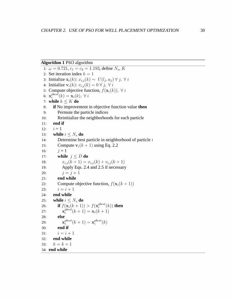
CHAPTER 2. USE OF PSO FOR WELL PLACEMENT OPTIMIZATION 30
Algorithm 1 PSO algorithm1: ω = 0.721, c1 = c2 = 1.193, defineNs, K2: Set iteration indexk = 13: Initialize xi(k): xi,j(k) ∼ U(lj, uj) ∀ j, ∀ i4: Initialize vi(k): vi,j(k) = 0 ∀ j, ∀ i5: Compute objective function,f(xi(k)), ∀ i6: x
pbesti (k) = xi(k), ∀ i
7: while k ≤ K do8: if No improvement in objective function valuethen9: Permute the particle indices
10: Reinitialize the neighborhoods for each particle11: end if12: i = 113: while i ≤ Ns do14: Determine best particle in neighborhood of particlei15: Computevi(k + 1) using Eq. 2.216: j = 117: while j ≤ D do18: xi,j(k + 1) = xi,j(k) + vi,j(k + 1)19: Apply Eqs. 2.4 and 2.5 if necessary20: j = j + 121: end while22: Compute objective function,f(xi(k + 1))23: i = i + 124: end while25: while i ≤ Ns do26: if f(xi(k + 1)) > f(xpbest
i (k)) then27: x
pbesti (k + 1) = xi(k + 1)
28: else29: x
pbesti (k + 1) = x
pbesti (k)
30: end if31: i = i + 132: end while33: k = k + 134: end while
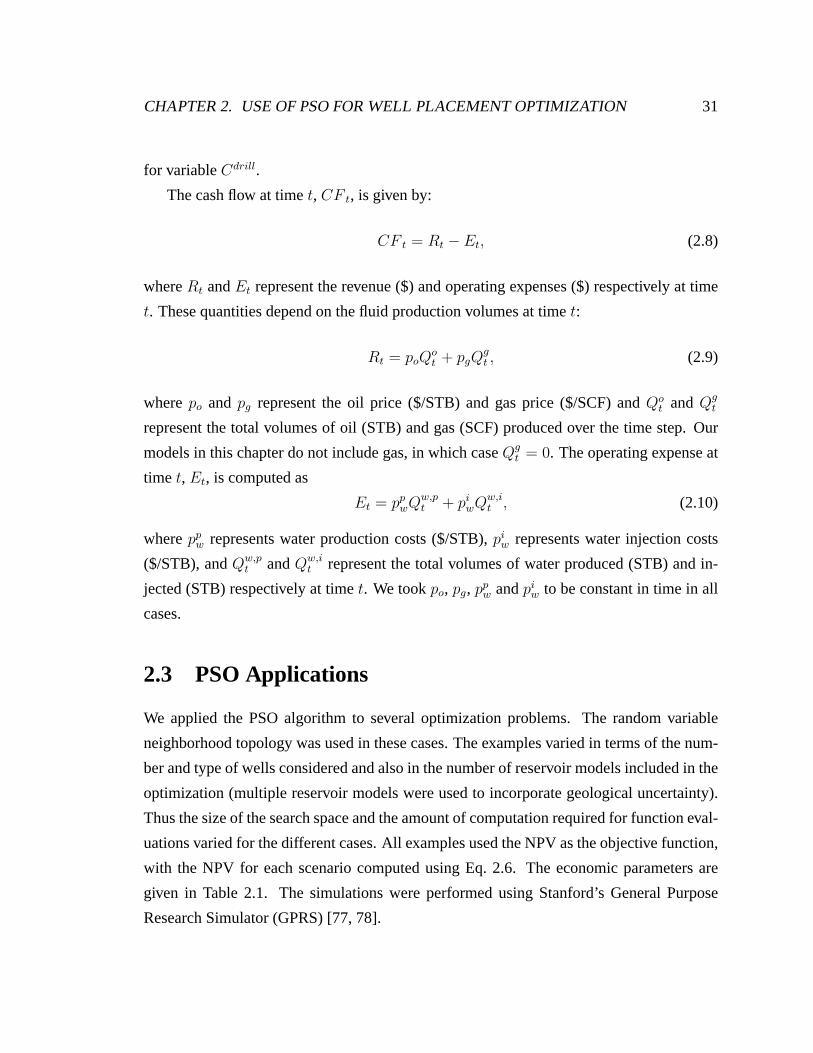
CHAPTER 2. USE OF PSO FOR WELL PLACEMENT OPTIMIZATION 31
for variableCdrill.
The cash flow at timet, CF t, is given by:
CF t = Rt − Et, (2.8)
whereRt andEt represent the revenue ($) and operating expenses ($) respectively at time
t. These quantities depend on the fluid production volumes at time t:
Rt = poQot + pgQ
gt , (2.9)
wherepo and pg represent the oil price ($/STB) and gas price ($/SCF) andQot andQg
t
represent the total volumes of oil (STB) and gas (SCF) producedover the time step. Our
models in this chapter do not include gas, in which caseQgt = 0. The operating expense at
time t, Et, is computed as
Et = ppwQw,p
t + piwQw,i
t , (2.10)
whereppw represents water production costs ($/STB),pi
w represents water injection costs
($/STB), andQw,pt andQw,i
t represent the total volumes of water produced (STB) and in-
jected (STB) respectively at timet. We tookpo, pg, ppw andpi
w to be constant in time in all
cases.
2.3 PSO Applications
We applied the PSO algorithm to several optimization problems. The random variable
neighborhood topology was used in these cases. The examplesvaried in terms of the num-
ber and type of wells considered and also in the number of reservoir models included in the
optimization (multiple reservoir models were used to incorporate geological uncertainty).
Thus the size of the search space and the amount of computation required for function eval-
uations varied for the different cases. All examples used the NPV as the objective function,
with the NPV for each scenario computed using Eq. 2.6. The economic parameters are
given in Table 2.1. The simulations were performed using Stanford’s General Purpose
Research Simulator (GPRS) [77, 78].
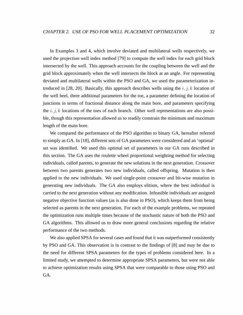
CHAPTER 2. USE OF PSO FOR WELL PLACEMENT OPTIMIZATION 32
In Examples 3 and 4, which involve deviated and multilateralwells respectively, we
used the projection well index method [79] to compute the well index for each grid block
intersected by the well. This approach accounts for the coupling between the well and the
grid block approximately when the well intersects the blockat an angle. For representing
deviated and multilateral wells within the PSO and GA, we used the parameterization in-
troduced in [28, 20]. Basically, this approach describes wells using thei, j, k location of
the well heel, three additional parameters for the toe, a parameter defining the location of
junctions in terms of fractional distance along the main bore, and parameters specifying
the i, j, k locations of the toes of each branch. Other well representations are also possi-
ble, though this representation allowed us to readily constrain the minimum and maximum
length of the main bore.
We compared the performance of the PSO algorithm to binary GA, hereafter referred
to simply as GA. In [18], different sets of GA parameters wereconsidered and an ‘optimal’
set was identified. We used this optimal set of parameters in our GA runs described in
this section. The GA uses the roulette wheel proportional weighting method for selecting
individuals, called parents, to generate the new solutionsin the next generation. Crossover
between two parents generates two new individuals, called offspring. Mutation is then
applied to the new individuals. We used single-point crossover and bit-wise mutation in
generating new individuals. The GA also employs elitism, where the best individual is
carried to the next generation without any modification. Infeasible individuals are assigned
negative objective function values (as is also done in PSO),which keeps them from being
selected as parents in the next generation. For each of the example problems, we repeated
the optimization runs multiple times because of the stochastic nature of both the PSO and
GA algorithms. This allowed us to draw more general conclusions regarding the relative
performance of the two methods.
We also applied SPSA for several cases and found that it was outperformed consistently
by PSO and GA. This observation is in contrast to the findings of [8] and may be due to
the need for different SPSA parameters for the types of problems considered here. In a
limited study, we attempted to determine appropriate SPSA parameters, but were not able
to achieve optimization results using SPSA that were comparable to those using PSO and
GA.
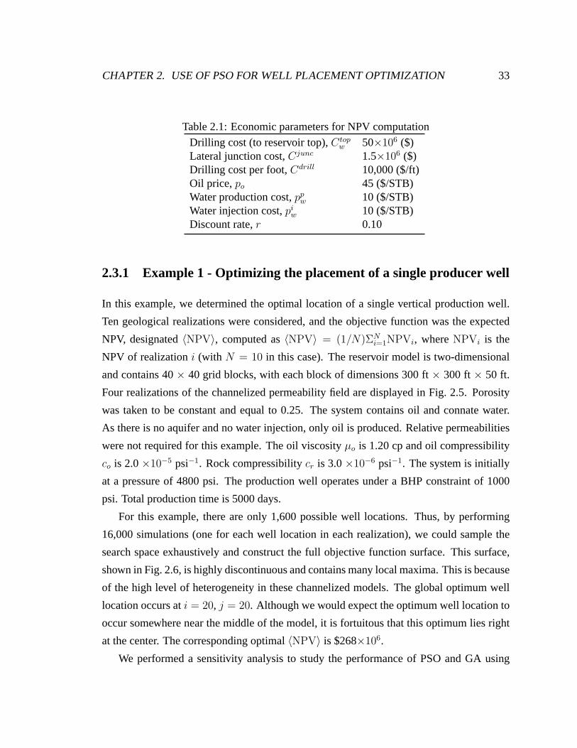
CHAPTER 2. USE OF PSO FOR WELL PLACEMENT OPTIMIZATION 33
Table 2.1: Economic parameters for NPV computation
Drilling cost (to reservoir top),Ctopw 50×106 ($)
Lateral junction cost,Cjunc 1.5×10⁶ ($)Drilling cost per foot,Cdrill 10,000 ($/ft)Oil price,po 45 ($/STB)Water production cost,pp
w 10 ($/STB)Water injection cost,pi
w 10 ($/STB)Discount rate,r 0.10
2.3.1 Example 1 - Optimizing the placement of a single producer well
In this example, we determined the optimal location of a single vertical production well.
Ten geological realizations were considered, and the objective function was the expected
NPV, designated〈NPV〉, computed as〈NPV〉 = (1/N)ΣNi=1
NPVi, whereNPVi is the
NPV of realizationi (with N = 10 in this case). The reservoir model is two-dimensional
and contains 40× 40 grid blocks, with each block of dimensions 300 ft× 300 ft× 50 ft.
Four realizations of the channelized permeability field aredisplayed in Fig. 2.5. Porosity
was taken to be constant and equal to 0.25. The system contains oil and connate water.
As there is no aquifer and no water injection, only oil is produced. Relative permeabilities
were not required for this example. The oil viscosityµo is 1.20 cp and oil compressibility
co is 2.0×10⁻⁵ psi−1. Rock compressibilitycr is 3.0×10⁻⁶ psi−1. The system is initially
at a pressure of 4800 psi. The production well operates undera BHP constraint of 1000
psi. Total production time is 5000 days.
For this example, there are only 1,600 possible well locations. Thus, by performing
16,000 simulations (one for each well location in each realization), we could sample the
search space exhaustively and construct the full objectivefunction surface. This surface,
shown in Fig. 2.6, is highly discontinuous and contains manylocal maxima. This is because
of the high level of heterogeneity in these channelized models. The global optimum well
location occurs ati = 20, j = 20. Although we would expect the optimum well location to
occur somewhere near the middle of the model, it is fortuitous that this optimum lies right
at the center. The corresponding optimal〈NPV〉 is $268×106.
We performed a sensitivity analysis to study the performance of PSO and GA using
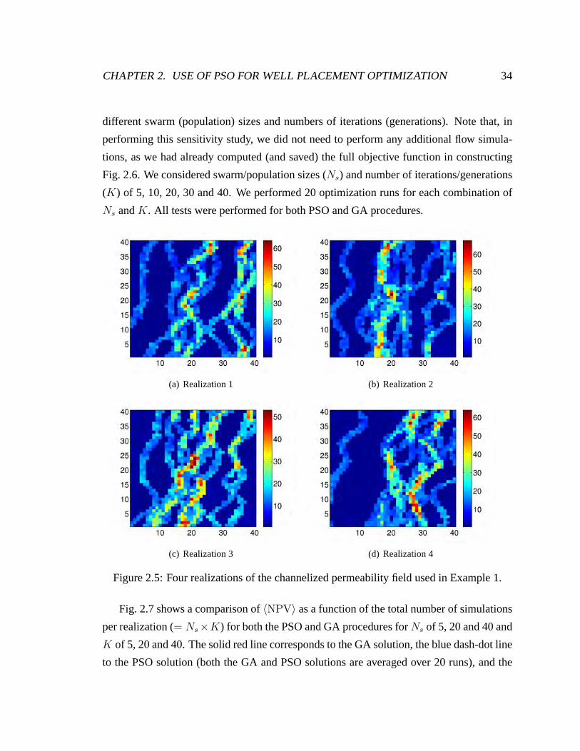
CHAPTER 2. USE OF PSO FOR WELL PLACEMENT OPTIMIZATION 34
different swarm (population) sizes and numbers of iterations (generations). Note that, in
performing this sensitivity study, we did not need to perform any additional flow simula-
tions, as we had already computed (and saved) the full objective function in constructing
Fig. 2.6. We considered swarm/population sizes (Ns) and number of iterations/generations
(K) of 5, 10, 20, 30 and 40. We performed 20 optimization runs foreach combination of
Ns andK. All tests were performed for both PSO and GA procedures.
(a) Realization 1 (b) Realization 2
(c) Realization 3 (d) Realization 4
Figure 2.5: Four realizations of the channelized permeability field used in Example 1.
Fig. 2.7 shows a comparison of〈NPV〉 as a function of the total number of simulations
per realization (= Ns×K) for both the PSO and GA procedures forNs of 5, 20 and 40 and
K of 5, 20 and 40. The solid red line corresponds to the GA solution, the blue dash-dot line
to the PSO solution (both the GA and PSO solutions are averaged over 20 runs), and the
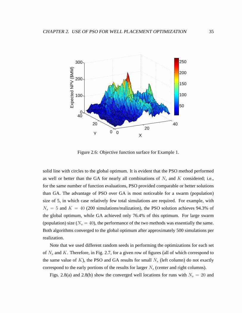
CHAPTER 2. USE OF PSO FOR WELL PLACEMENT OPTIMIZATION 35
020
40
0
20
400
100
200
300
XY
Exp
ecte
d N
PV
($M
M)
50
100
150
200
250
Figure 2.6: Objective function surface for Example 1.
solid line with circles to the global optimum. It is evident that the PSO method performed
as well or better than the GA for nearly all combinations ofNs andK considered; i.e.,
for the same number of function evaluations, PSO provided comparable or better solutions
than GA. The advantage of PSO over GA is most noticeable for a swarm (population)
size of 5, in which case relatively few total simulations arerequired. For example, with
Ns = 5 andK = 40 (200 simulations/realization), the PSO solution achieves94.3% of
the global optimum, while GA achieved only 76.4% of this optimum. For large swarm
(population) size (Ns = 40), the performance of the two methods was essentially the same.
Both algorithms converged to the global optimum after approximately 500 simulations per
realization.
Note that we used different random seeds in performing the optimizations for each set
of Ns andK. Therefore, in Fig. 2.7, for a given row of figures (all of which correspond to
the same value ofK), the PSO and GA results for smallNs (left column) do not exactly
correspond to the early portions of the results for largerNs (center and right columns).
Figs. 2.8(a) and 2.8(b) show the converged well locations for runs withNs = 20 and
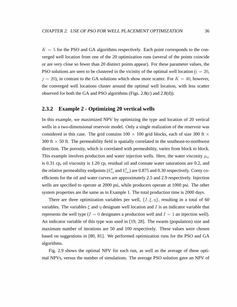
CHAPTER 2. USE OF PSO FOR WELL PLACEMENT OPTIMIZATION 36
K = 5 for the PSO and GA algorithms respectively. Each point corresponds to the con-
verged well location from one of the 20 optimization runs (several of the points coincide
or are very close so fewer than 20 distinct points appear). For these parameter values, the
PSO solutions are seen to be clustered in the vicinity of the optimal well location (i = 20,
j = 20), in contrast to the GA solutions which show more scatter. For K = 40, however,
the converged well locations cluster around the optimal well location, with less scatter
observed for both the GA and PSO algorithms (Figs. 2.8(c) and2.8(d)).
2.3.2 Example 2 - Optimizing 20 vertical wells
In this example, we maximized NPV by optimizing the type and location of 20 vertical
wells in a two-dimensional reservoir model. Only a single realization of the reservoir was
considered in this case. The grid contains 100× 100 grid blocks, each of size 300 ft×
300 ft× 50 ft. The permeability field is spatially correlated in the southeast-to-northwest
direction. The porosity, which is correlated with permeability, varies from block to block.
This example involves production and water injection wells. Here, the water viscosityµw
is 0.31 cp, oil viscosity is 1.20 cp, residual oil and connatewater saturations are 0.2, and
the relative permeability endpoints (k0
ro andk0
rw) are 0.875 and 0.30 respectively. Corey co-
efficients for the oil and water curves are approximately 2.5and 2.9 respectively. Injection
wells are specified to operate at 2000 psi, while producers operate at 1000 psi. The other
system properties are the same as in Example 1. The total production time is 2000 days.
There are three optimization variables per well,{I, ξ, η}, resulting in a total of 60
variables. The variablesξ andη designate well location andI is an indicator variable that
represents the well type (I = 0 designates a production well andI = 1 an injection well).
An indicator variable of this type was used in [19, 28]. The swarm (population) size and
maximum number of iterations are 50 and 100 respectively. These values were chosen
based on suggestions in [80, 81]. We performed optimizationruns for the PSO and GA
algorithms.
Fig. 2.9 shows the optimal NPV for each run, as well as the average of these opti-
mal NPVs, versus the number of simulations. The average PSO solution gave an NPV of
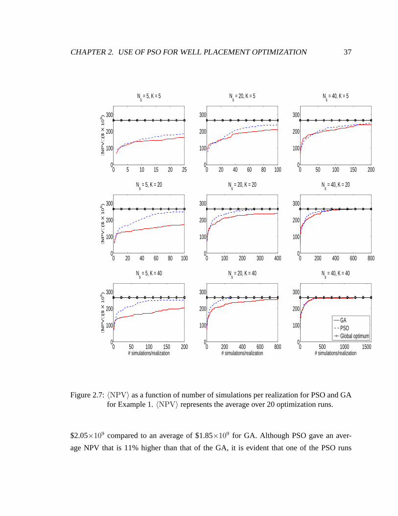
CHAPTER 2. USE OF PSO FOR WELL PLACEMENT OPTIMIZATION 37
0 5 10 15 20 250
100
200
300
⟨NP
V⟩
($ X
10
6)
Ns = 5, K = 5
0 20 40 60 80 1000
100
200
300
Ns = 20, K = 5
0 50 100 150 2000
100
200
300
Ns = 40, K = 5
0 20 40 60 80 1000
100
200
300
⟨NP
V⟩
($ X
10
6)
Ns = 5, K = 20
0 100 200 300 4000
100
200
300
Ns = 20, K = 20
0 200 400 600 8000
100
200
300
Ns = 40, K = 20
0 50 100 150 2000
100
200
300
# simulations/realization
⟨NP
V⟩
($ X
10
6)
Ns = 5, K = 40
0 200 400 600 8000
100
200
300
# simulations/realization
Ns = 20, K = 40
0 500 1000 15000
100
200
300
# simulations/realization
Ns = 40, K = 40
GAPSOGlobal optimum
Figure 2.7:〈NPV〉 as a function of number of simulations per realization for PSO and GAfor Example 1.〈NPV〉 represents the average over 20 optimization runs.
$2.05×10⁹ compared to an average of $1.85×10⁹ for GA. Although PSO gave an aver-
age NPV that is 11% higher than that of the GA, it is evident that one of the PSO runs
CHAPTER 2. USE OF PSO FOR WELL PLACEMENT OPTIMIZATION 38
0 10 20 30 400
5
10
15
20
25
30
35
40
X
Y
(a) PSO:Ns = 20,K = 5
0 10 20 30 400
5
10
15
20
25
30
35
40
X
Y
(b) GA: Ns = 20,K = 5
0 10 20 30 400
5
10
15
20
25
30
35
40
X
Y
(c) PSO:Ns = 20,K = 40
0 10 20 30 400
5
10
15
20
25
30
35
40
X
Y
(d) GA: Ns = 20,K = 40
Figure 2.8: Optimal well locations from PSO and GA forNs = 20, and for number ofiterationsK = 5 (top row), andK = 40 (bottom row). Each point correspondsto the well location from one of the 20 optimization runs (Example 1).
gave a fairly low NPV. This highlights the need for multiple runs. Note that, in these and
subsequent results, during the course of the optimizations, around 5% of the scenarios had
invalid well configurations. For these cases we did not perform flow simulations, but we
still included them in the total simulation count.
The optimal well locations for the highest NPV case using PSOare shown in Fig. 2.10(a).
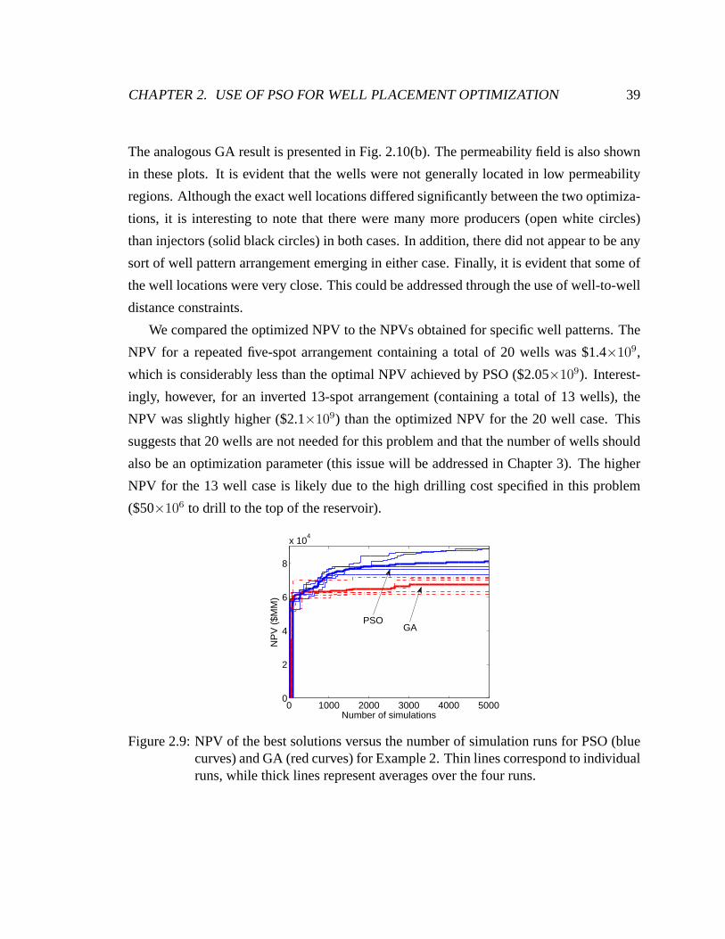
CHAPTER 2. USE OF PSO FOR WELL PLACEMENT OPTIMIZATION 39
The analogous GA result is presented in Fig. 2.10(b). The permeability field is also shown
in these plots. It is evident that the wells were not generally located in low permeability
regions. Although the exact well locations differed significantly between the two optimiza-
tions, it is interesting to note that there were many more producers (open white circles)
than injectors (solid black circles) in both cases. In addition, there did not appear to be any
sort of well pattern arrangement emerging in either case. Finally, it is evident that some of
the well locations were very close. This could be addressed through the use of well-to-well
distance constraints.
We compared the optimized NPV to the NPVs obtained for specific well patterns. The
NPV for a repeated five-spot arrangement containing a total of 20 wells was $1.4×10⁹,
which is considerably less than the optimal NPV achieved by PSO ($2.05×10⁹). Interest-
ingly, however, for an inverted 13-spot arrangement (containing a total of 13 wells), the
NPV was slightly higher ($2.1×10⁹) than the optimized NPV for the 20 well case. This
suggests that 20 wells are not needed for this problem and that the number of wells should
also be an optimization parameter (this issue will be addressed in Chapter 3). The higher
NPV for the 13 well case is likely due to the high drilling costspecified in this problem
($50×106 to drill to the top of the reservoir).
0 1000 2000 3000 4000 50000
2
4
6
8
x 104
Number of simulations
NP
V (
$MM
)
GAPSO
Figure 2.9: NPV of the best solutions versus the number of simulation runs for PSO (bluecurves) and GA (red curves) for Example 2. Thin lines correspond to individualruns, while thick lines represent averages over the four runs.

CHAPTER 2. USE OF PSO FOR WELL PLACEMENT OPTIMIZATION 40
X
Y
20 40 60 80 100
20
40
60
80
100
200
400
600
800
(a) PSO
X
Y
20 40 60 80 100
20
40
60
80
100
200
400
600
800
(b) GA
Figure 2.10: Permeability field and well locations from the best runs using PSO and GAfor Example 2. The open white circles correspond to producers and the solidblack circles to injectors.
2.3.3 Example 3 - Optimizing four deviated producers
This example entails the determination of the optimal location for four deviated monobore
producer wells. The reservoir model contains 63× 63× 7 grid blocks, each of dimensions
60 ft × 60 ft × 20 ft. The other reservoir properties are the same as in previous examples.
We consider only a single realization of the reservoir; the permeability field is shown in
Fig. 2.11.
Each deviated well is represented by six optimization variables, resulting in a total of 24
variables. The maximum possible length of any well is specified to be 2500 ft. Additional
constraints are also included. For example, if the main bores for any two wells intersect, the
solution is considered invalid (see Section 2.1.2 for explanation of our treatment of invalid
solutions).
We performed five optimization runs for each algorithm. Fig.2.12 shows the optimal
results for each run and the average of these solutions versus the number of simulations.
The averaged NPV for the PSO and GA algorithms are $479×106 and $448×106 respec-
tively. Thus the average PSO solution is 7% higher than the average GA solution. The
converged well locations from the best run for both algorithms are shown in Fig. 2.13. The
results consist of deviated and nearly horizontal wells, though the two solutions differ in
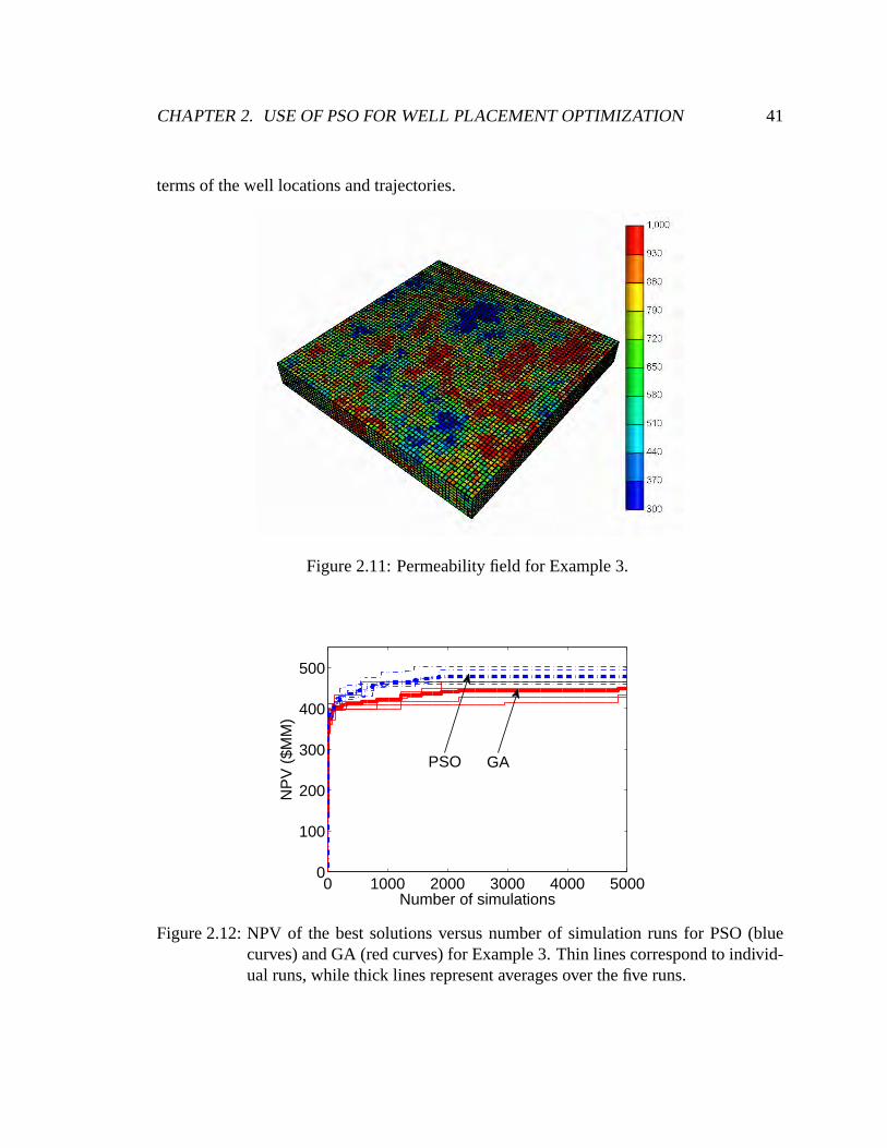
CHAPTER 2. USE OF PSO FOR WELL PLACEMENT OPTIMIZATION 41
terms of the well locations and trajectories.
Figure 2.11: Permeability field for Example 3.
0 1000 2000 3000 4000 50000
100
200
300
400
500
Number of simulations
NP
V (
$MM
)
GAPSO
Figure 2.12: NPV of the best solutions versus number of simulation runs for PSO (bluecurves) and GA (red curves) for Example 3. Thin lines correspond to individ-ual runs, while thick lines represent averages over the five runs.
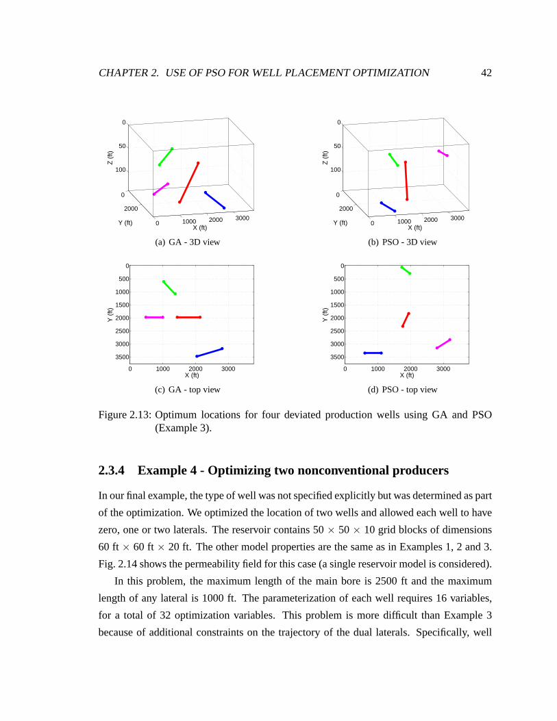
CHAPTER 2. USE OF PSO FOR WELL PLACEMENT OPTIMIZATION 42
0 1000 2000 3000
0
2000
0
50
100
X (ft)Y (ft)
Z (
ft)
(a) GA - 3D view
0 1000 2000 3000
0
2000
0
50
100
X (ft)Y (ft)
Z (
ft)
(b) PSO - 3D view
0 1000 2000 3000
0
500
1000
1500
2000
2500
3000
3500
X (ft)
Y (
ft)
(c) GA - top view
0 1000 2000 3000
0
500
1000
1500
2000
2500
3000
3500
X (ft)
Y (
ft)
(d) PSO - top view
Figure 2.13: Optimum locations for four deviated production wells using GA and PSO(Example 3).
2.3.4 Example 4 - Optimizing two nonconventional producers
In our final example, the type of well was not specified explicitly but was determined as part
of the optimization. We optimized the location of two wells and allowed each well to have
zero, one or two laterals. The reservoir contains 50× 50× 10 grid blocks of dimensions
60 ft × 60 ft × 20 ft. The other model properties are the same as in Examples 1, 2 and 3.
Fig. 2.14 shows the permeability field for this case (a singlereservoir model is considered).
In this problem, the maximum length of the main bore is 2500 ftand the maximum
length of any lateral is 1000 ft. The parameterization of each well requires 16 variables,
for a total of 32 optimization variables. This problem is more difficult than Example 3
because of additional constraints on the trajectory of the dual laterals. Specifically, well
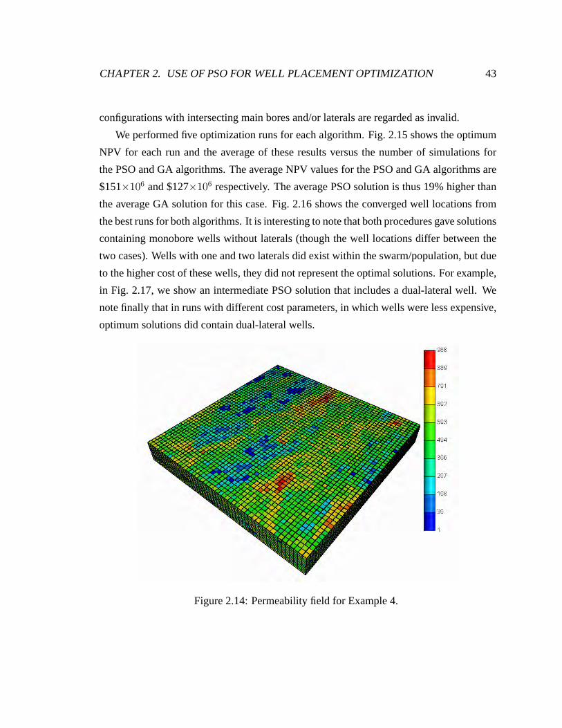
CHAPTER 2. USE OF PSO FOR WELL PLACEMENT OPTIMIZATION 43
configurations with intersecting main bores and/or laterals are regarded as invalid.
We performed five optimization runs for each algorithm. Fig.2.15 shows the optimum
NPV for each run and the average of these results versus the number of simulations for
the PSO and GA algorithms. The average NPV values for the PSO and GA algorithms are
$151×106 and $127×106 respectively. The average PSO solution is thus 19% higher than
the average GA solution for this case. Fig. 2.16 shows the converged well locations from
the best runs for both algorithms. It is interesting to note that both procedures gave solutions
containing monobore wells without laterals (though the well locations differ between the
two cases). Wells with one and two laterals did exist within the swarm/population, but due
to the higher cost of these wells, they did not represent the optimal solutions. For example,
in Fig. 2.17, we show an intermediate PSO solution that includes a dual-lateral well. We
note finally that in runs with different cost parameters, in which wells were less expensive,
optimum solutions did contain dual-lateral wells.
Figure 2.14: Permeability field for Example 4.
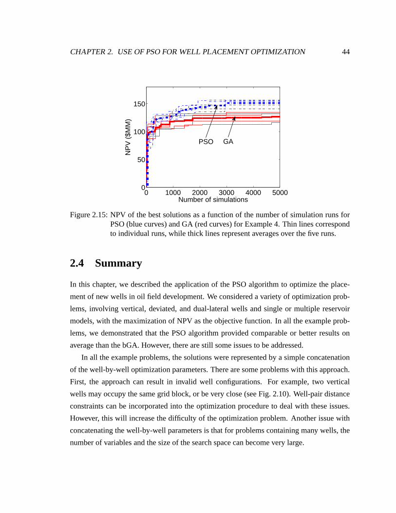
CHAPTER 2. USE OF PSO FOR WELL PLACEMENT OPTIMIZATION 44
0 1000 2000 3000 4000 50000
50
100
150
Number of simulations
NP
V (
$MM
)
PSO GA
Figure 2.15: NPV of the best solutions as a function of the number of simulation runs forPSO (blue curves) and GA (red curves) for Example 4. Thin lines correspondto individual runs, while thick lines represent averages over the five runs.
2.4 Summary
In this chapter, we described the application of the PSO algorithm to optimize the place-
ment of new wells in oil field development. We considered a variety of optimization prob-
lems, involving vertical, deviated, and dual-lateral wells and single or multiple reservoir
models, with the maximization of NPV as the objective function. In all the example prob-
lems, we demonstrated that the PSO algorithm provided comparable or better results on
average than the bGA. However, there are still some issues tobe addressed.
In all the example problems, the solutions were representedby a simple concatenation
of the well-by-well optimization parameters. There are some problems with this approach.
First, the approach can result in invalid well configurations. For example, two vertical
wells may occupy the same grid block, or be very close (see Fig. 2.10). Well-pair distance
constraints can be incorporated into the optimization procedure to deal with these issues.
However, this will increase the difficulty of the optimization problem. Another issue with
concatenating the well-by-well parameters is that for problems containing many wells, the
number of variables and the size of the search space can become very large.
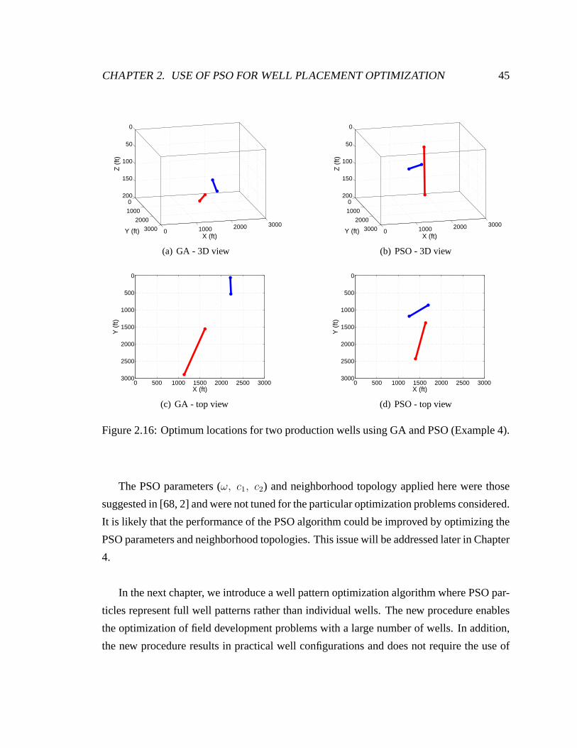
CHAPTER 2. USE OF PSO FOR WELL PLACEMENT OPTIMIZATION 45
0 1000 2000 3000
0
1000
2000
3000
0
50
100
150
200
X (ft)Y (ft)
Z (
ft)
(a) GA - 3D view
0 1000 2000 3000
0
1000
2000
3000
0
50
100
150
200
X (ft)Y (ft)
Z (
ft)
(b) PSO - 3D view
0 500 1000 1500 2000 2500 3000
0
500
1000
1500
2000
2500
3000
X (ft)
Y (
ft)
(c) GA - top view
0 500 1000 1500 2000 2500 3000
0
500
1000
1500
2000
2500
3000
X (ft)
Y (
ft)
(d) PSO - top view
Figure 2.16: Optimum locations for two production wells using GA and PSO (Example 4).
The PSO parameters (ω, c1, c2) and neighborhood topology applied here were those
suggested in [68, 2] and were not tuned for the particular optimization problems considered.
It is likely that the performance of the PSO algorithm could be improved by optimizing the
PSO parameters and neighborhood topologies. This issue will be addressed later in Chapter
4.
In the next chapter, we introduce a well pattern optimization algorithm where PSO par-
ticles represent full well patterns rather than individualwells. The new procedure enables
the optimization of field development problems with a large number of wells. In addition,
the new procedure results in practical well configurations and does not require the use of
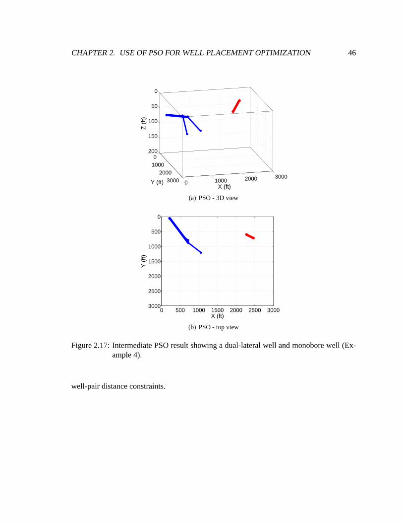
CHAPTER 2. USE OF PSO FOR WELL PLACEMENT OPTIMIZATION 46
0 1000 2000 3000
01000
20003000
0
50
100
150
200
X (ft)Y (ft)
Z (
ft)
(a) PSO - 3D view
0 500 1000 1500 2000 2500 3000
0
500
1000
1500
2000
2500
3000
X (ft)
Y (
ft)
(b) PSO - top view
Figure 2.17: Intermediate PSO result showing a dual-lateral well and monobore well (Ex-ample 4).
well-pair distance constraints.
Chapter 3
Well Pattern Optimization
In this chapter, we present a new procedure for optimizing large-scale field development,
called well pattern optimization (WPO). WPO consists of threemain components: well
pattern description (WPD), well-by-well perturbation (WWP),and the PSO algorithm. In
this chapter, we first describe the WPD, which is a novel representation for well patterns.
The components of WPD, which include a generic representation for different well pattern
types and applicable pattern operators (rotation, scale, shear and switch), are discussed.
Next, we present the well-by-well perturbation (WWP) which can be used to improve the
solutions obtained using WPD. Several example problems wereconsidered using the WPO
procedure. In total, these results demonstrate the applicability of WPO for large-scale field
development.
3.1 Well Pattern Description (WPD)
The overall well pattern optimization (WPO) algorithm contains as key components the
well pattern description (WPD), well-by-well perturbation, and the core optimization algo-
rithm (PSO in this case). The WPD, which we now describe, treats well patterns (rather
than individual wells) as the basic unit of representation.Thus, in our PSO implementa-
tion, each particle represents a repeated well pattern. WPD can encode representations for
a wide variety of possible well patterns, in addition to the transformations that are used to
manipulate these well patterns. It is the parameters that define the patterns and quantify
47
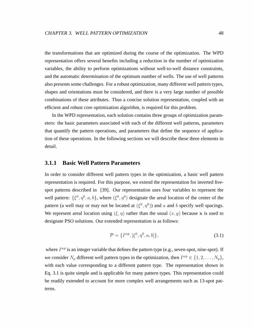
CHAPTER 3. WELL PATTERN OPTIMIZATION 48
the transformations that are optimized during the course ofthe optimization. The WPD
representation offers several benefits including a reduction in the number of optimization
variables, the ability to perform optimizations without well-to-well distance constraints,
and the automatic determination of the optimum number of wells. The use of well patterns
also presents some challenges. For a robust optimization, many different well pattern types,
shapes and orientations must be considered, and there is a very large number of possible
combinations of these attributes. Thus a concise solution representation, coupled with an
efficient and robust core optimization algorithm, is required for this problem.
In the WPD representation, each solution contains three groups of optimization param-
eters: the basic parameters associated with each of the different well patterns, parameters
that quantify the pattern operations, and parameters that define the sequence of applica-
tion of these operations. In the following sections we will describe these three elements in
detail.
3.1.1 Basic Well Pattern Parameters
In order to consider different well pattern types in the optimization, a basic well pattern
representation is required. For this purpose, we extend therepresentation for inverted five-
spot patterns described in [39]. Our representation uses four variables to represent the
well pattern:{ξ0, η0, a, b}, where(ξ0, η0) designate the areal location of the center of the
pattern (a well may or may not be located at(ξ0, η0)) anda andb specify well spacings.
We represent areal location using(ξ, η) rather than the usual(x, y) becausex is used to
designate PSO solutions. Our extended representation is asfollows:
P = {Iwp, [ξ0, η0, a, b]}, (3.1)
whereIwp is an integer variable that defines the pattern type (e.g., seven-spot, nine-spot). If
we considerNp different well pattern types in the optimization, thenIwp ∈ {1, 2, . . . , Np},
with each value corresponding to a different pattern type. The representation shown in
Eq. 3.1 is quite simple and is applicable for many pattern types. This representation could
be readily extended to account for more complex well arrangements such as 13-spot pat-
terns.
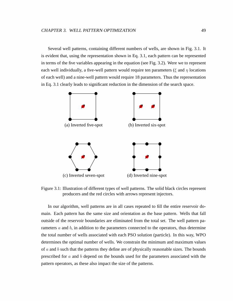
CHAPTER 3. WELL PATTERN OPTIMIZATION 49
Several well patterns, containing different numbers of wells, are shown in Fig. 3.1. It
is evident that, using the representation shown in Eq. 3.1, each pattern can be represented
in terms of the five variables appearing in the equation (see Fig. 3.2). Were we to represent
each well individually, a five-well pattern would require ten parameters (ξ andη locations
of each well) and a nine-well pattern would require 18 parameters. Thus the representation
in Eq. 3.1 clearly leads to significant reduction in the dimension of the search space.
(a) Inverted five-spot (b) Inverted six-spot
(c) Inverted seven-spot (d) Inverted nine-spot
Figure 3.1: Illustration of different types of well patterns. The solid black circles representproducers and the red circles with arrows represent injectors.
In our algorithm, well patterns are in all cases repeated to fill the entire reservoir do-
main. Each pattern has the same size and orientation as the base pattern. Wells that fall
outside of the reservoir boundaries are eliminated from thetotal set. The well pattern pa-
rametersa andb, in addition to the parameters connected to the operators, thus determine
the total number of wells associated with each PSO solution (particle). In this way, WPO
determines the optimal number of wells. We constrain the minimum and maximum values
of a andb such that the patterns they define are of physically reasonable sizes. The bounds
prescribed fora andb depend on the bounds used for the parameters associated withthe
pattern operators, as these also impact the size of the patterns.
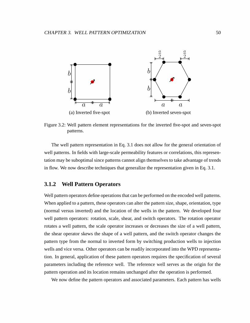
CHAPTER 3. WELL PATTERN OPTIMIZATION 50
b
b
a a
b
b
a a
a2
a2
(a) Inverted five-spot (b) Inverted seven-spot
Figure 3.2: Well pattern element representations for the inverted five-spot and seven-spotpatterns.
The well pattern representation in Eq. 3.1 does not allow forthe general orientation of
well patterns. In fields with large-scale permeability features or correlations, this represen-
tation may be suboptimal since patterns cannot align themselves to take advantage of trends
in flow. We now describe techniques that generalize the representation given in Eq. 3.1.
3.1.2 Well Pattern Operators
Well pattern operators define operations that can be performed on the encoded well patterns.
When applied to a pattern, these operators can alter the pattern size, shape, orientation, type
(normal versus inverted) and the location of the wells in thepattern. We developed four
well pattern operators: rotation, scale, shear, and switchoperators. The rotation operator
rotates a well pattern, the scale operator increases or decreases the size of a well pattern,
the shear operator skews the shape of a well pattern, and the switch operator changes the
pattern type from the normal to inverted form by switching production wells to injection
wells and vice versa. Other operators can be readily incorporated into the WPD representa-
tion. In general, application of these pattern operators requires the specification of several
parameters including the reference well. The reference well serves as the origin for the
pattern operation and its location remains unchanged afterthe operation is performed.
We now define the pattern operators and associated parameters. Each pattern has wells
CHAPTER 3. WELL PATTERN OPTIMIZATION 51
located at the vertices of a polygon (outer wells) and, except for the six-spot pattern, there
is also a well at the center (Fig. 3.1). In our numbering convention, the outer wells are
numbered consecutively in the anticlockwise direction followed by the interior well(s).
Each pattern operator takes as input a well pattern and produces a new well pattern as
output. We designateWin to be anN × 2 matrix representing the well locations in the
input well pattern element (these well locations are designated(ξ, η)) andWout to be the
corresponding matrix representing the output well locations (designated(ξ, η)). In both
matrices, well locations are relative to the reference well, located at(ξref , ηref ). The two
matrices are given by:
Win =
ξ1 − ξref η1 − ηref
ξ2 − ξref η2 − ηref
......
ξn − ξref ηn − ηref
......
ξNwp− ξref ηNwp
− ηref
, Wout =
ξ1 − ξref η1 − ηref
ξ2 − ξref η2 − ηref
......
ξn − ξref ηn − ηref
......
ξNwp− ξref ηNwp
− ηref
,
(3.2)
whereNwp is the number of wells in the well pattern. Most of the well pattern transforma-
tions can now be described through the following operation:
WTout = M W
Tin, (3.3)
whereM is a2× 2 transformation matrix. The specific forms ofM for the relevant pattern
operators are described below. We illustrate the well pattern operators using the inverted
five-spot and seven-spot well patterns, though the operators also apply to the other well
pattern types.
Rotation operator
The rotation operator, designatedOrot, rotates a well pattern by an angleθ about a reference
well, nref , nref ∈ {1, 2, . . . , Nwp}. After the rotation, the locations of all wells other than
nref are altered. The rotation operator does not change the size of the well pattern. The
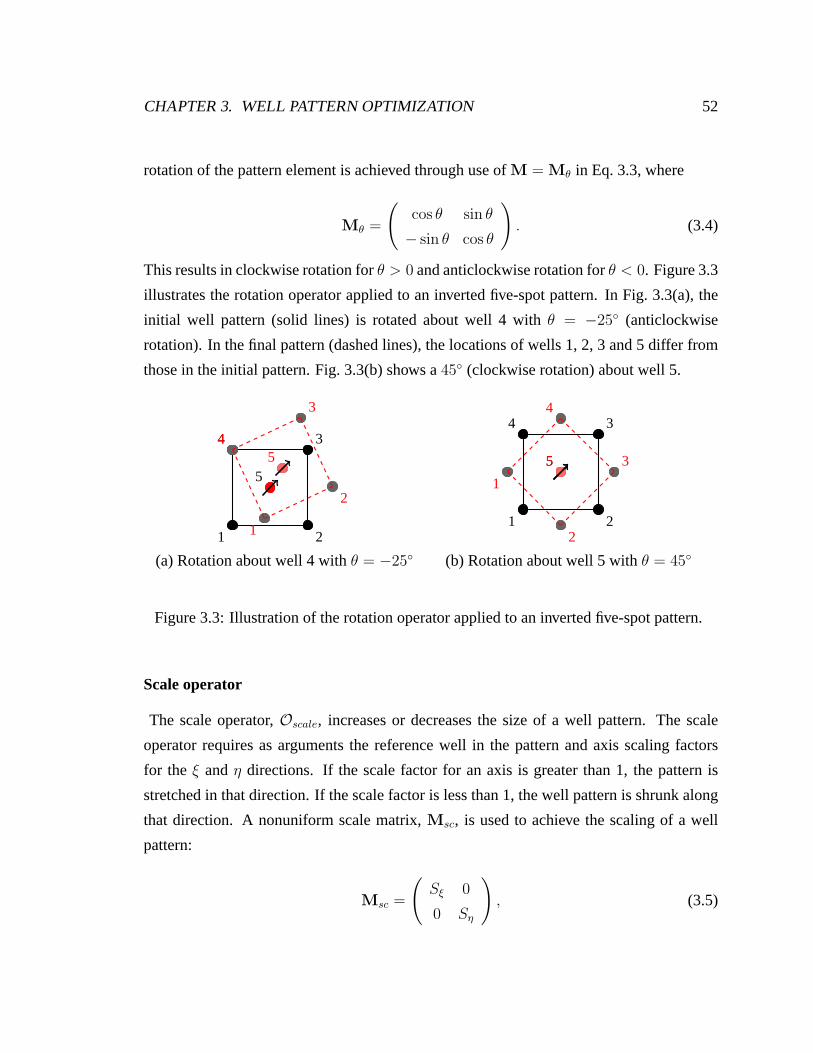
CHAPTER 3. WELL PATTERN OPTIMIZATION 52
rotation of the pattern element is achieved through use ofM = Mθ in Eq. 3.3, where
Mθ =
(
cos θ sin θ
− sin θ cos θ
)
. (3.4)
This results in clockwise rotation forθ > 0 and anticlockwise rotation forθ < 0. Figure 3.3
illustrates the rotation operator applied to an inverted five-spot pattern. In Fig. 3.3(a), the
initial well pattern (solid lines) is rotated about well 4 with θ = −25◦ (anticlockwise
rotation). In the final pattern (dashed lines), the locations of wells 1, 2, 3 and 5 differ from
those in the initial pattern. Fig. 3.3(b) shows a45◦ (clockwise rotation) about well 5.
1 2
34
5
1
2
3
45
1 2
34
5
1
2
3
4
5
(a) Rotation about well 4 withθ = −25◦ (b) Rotation about well 5 withθ = 45◦
Figure 3.3: Illustration of the rotation operator applied to an inverted five-spot pattern.
Scale operator
The scale operator,Oscale, increases or decreases the size of a well pattern. The scale
operator requires as arguments the reference well in the pattern and axis scaling factors
for the ξ andη directions. If the scale factor for an axis is greater than 1,the pattern is
stretched in that direction. If the scale factor is less than1, the well pattern is shrunk along
that direction. A nonuniform scale matrix,Msc, is used to achieve the scaling of a well
pattern:
Msc =
(
Sξ 0
0 Sη
)
, (3.5)
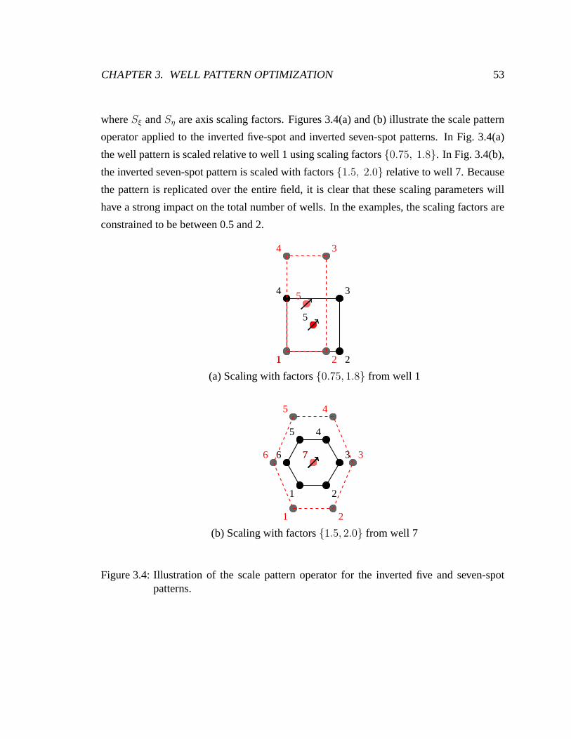
CHAPTER 3. WELL PATTERN OPTIMIZATION 53
whereSξ andSη are axis scaling factors. Figures 3.4(a) and (b) illustratethe scale pattern
operator applied to the inverted five-spot and inverted seven-spot patterns. In Fig. 3.4(a)
the well pattern is scaled relative to well 1 using scaling factors{0.75, 1.8}. In Fig. 3.4(b),
the inverted seven-spot pattern is scaled with factors{1.5, 2.0} relative to well 7. Because
the pattern is replicated over the entire field, it is clear that these scaling parameters will
have a strong impact on the total number of wells. In the examples, the scaling factors are
constrained to be between 0.5 and 2.
1 2
34
5
1 2
34
5
(a) Scaling with factors{0.75, 1.8} from well 1
1 2
3
45
6 7
1 2
3
45
6 7
(b) Scaling with factors{1.5, 2.0} from well 7
Figure 3.4: Illustration of the scale pattern operator for the inverted five and seven-spotpatterns.
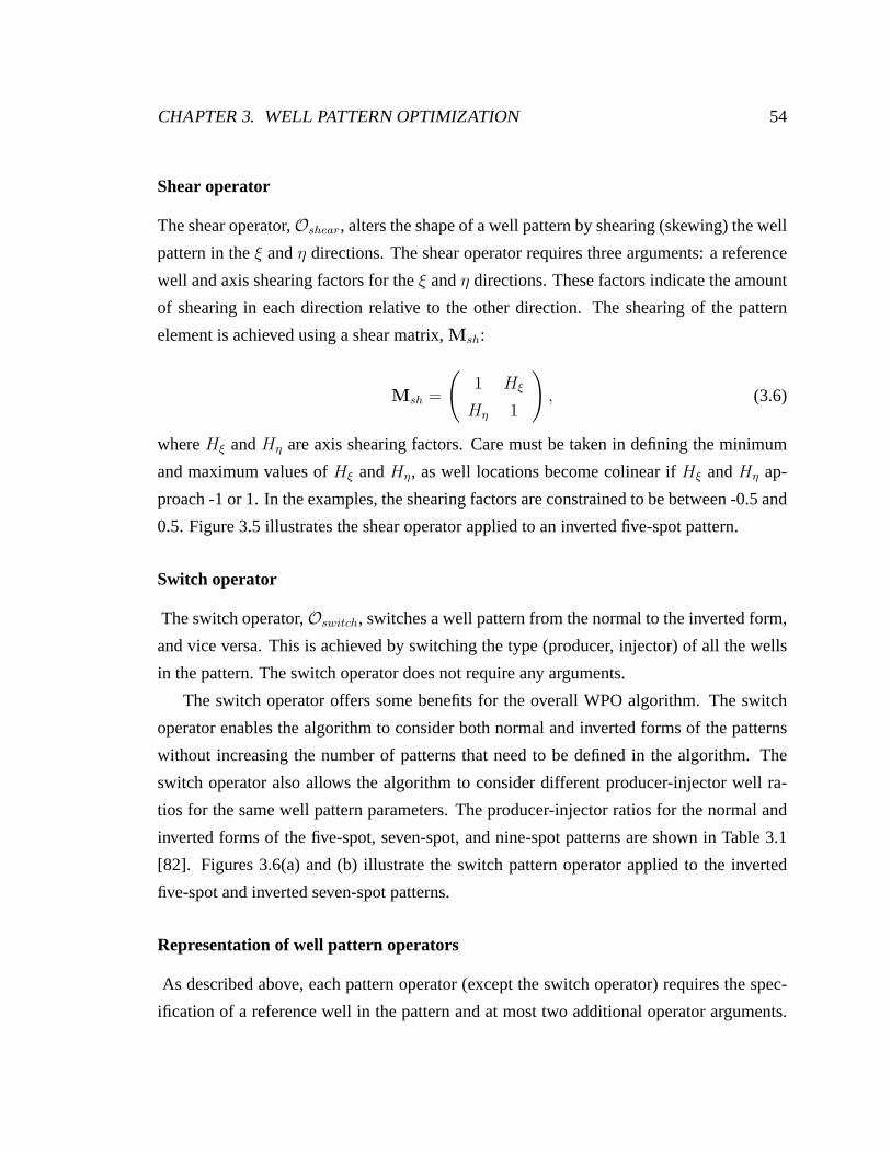
CHAPTER 3. WELL PATTERN OPTIMIZATION 54
Shear operator
The shear operator,Oshear, alters the shape of a well pattern by shearing (skewing) thewell
pattern in theξ andη directions. The shear operator requires three arguments: areference
well and axis shearing factors for theξ andη directions. These factors indicate the amount
of shearing in each direction relative to the other direction. The shearing of the pattern
element is achieved using a shear matrix,Msh:
Msh =
(
1 Hξ
Hη 1
)
, (3.6)
whereHξ andHη are axis shearing factors. Care must be taken in defining the minimum
and maximum values ofHξ andHη, as well locations become colinear ifHξ andHη ap-
proach -1 or 1. In the examples, the shearing factors are constrained to be between -0.5 and
0.5. Figure 3.5 illustrates the shear operator applied to aninverted five-spot pattern.
Switch operator
The switch operator,Oswitch, switches a well pattern from the normal to the inverted form,
and vice versa. This is achieved by switching the type (producer, injector) of all the wells
in the pattern. The switch operator does not require any arguments.
The switch operator offers some benefits for the overall WPO algorithm. The switch
operator enables the algorithm to consider both normal and inverted forms of the patterns
without increasing the number of patterns that need to be defined in the algorithm. The
switch operator also allows the algorithm to consider different producer-injector well ra-
tios for the same well pattern parameters. The producer-injector ratios for the normal and
inverted forms of the five-spot, seven-spot, and nine-spot patterns are shown in Table 3.1
[82]. Figures 3.6(a) and (b) illustrate the switch pattern operator applied to the inverted
five-spot and inverted seven-spot patterns.
Representation of well pattern operators
As described above, each pattern operator (except the switch operator) requires the spec-
ification of a reference well in the pattern and at most two additional operator arguments.
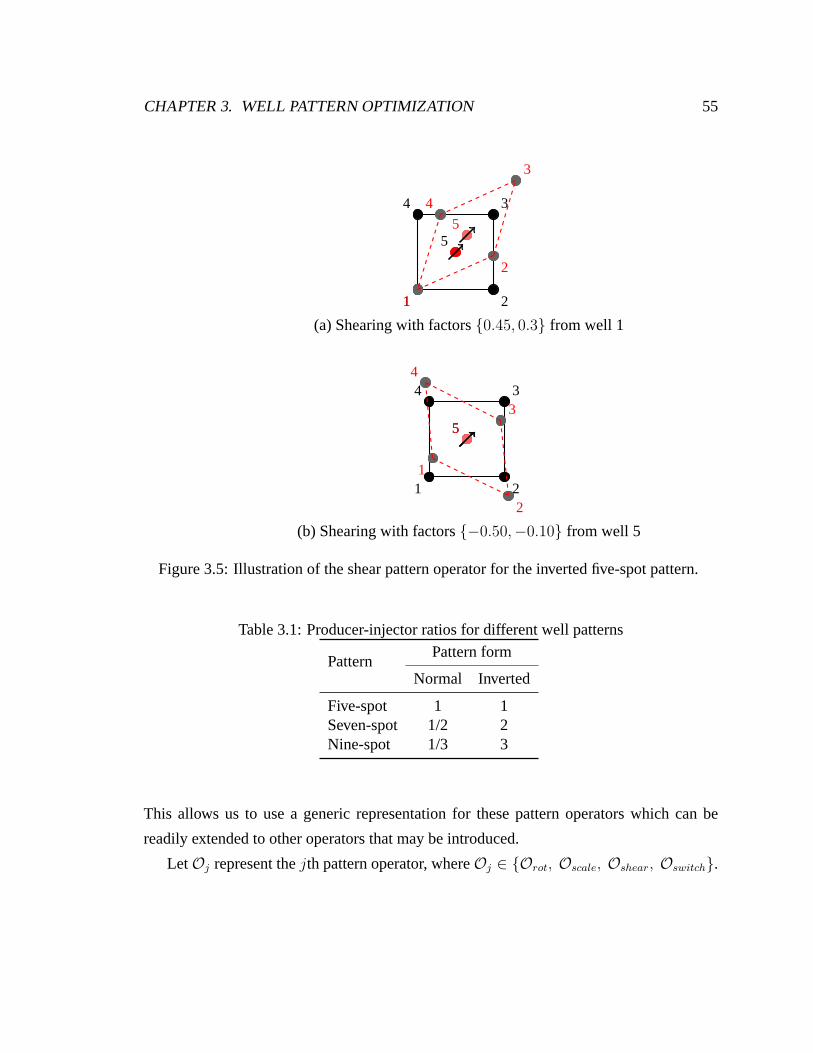
CHAPTER 3. WELL PATTERN OPTIMIZATION 55
1 2
34
5
1
2
3
4
5
(a) Shearing with factors{0.45, 0.3} from well 1
1 2
34
5
1
2
3
4
5
(b) Shearing with factors{−0.50,−0.10} from well 5
Figure 3.5: Illustration of the shear pattern operator for the inverted five-spot pattern.
Table 3.1: Producer-injector ratios for different well patterns
PatternPattern form
Normal Inverted
Five-spot 1 1Seven-spot 1/2 2Nine-spot 1/3 3
This allows us to use a generic representation for these pattern operators which can be
readily extended to other operators that may be introduced.
LetOj represent thejth pattern operator, whereOj ∈ {Orot, Oscale, Oshear, Oswitch}.
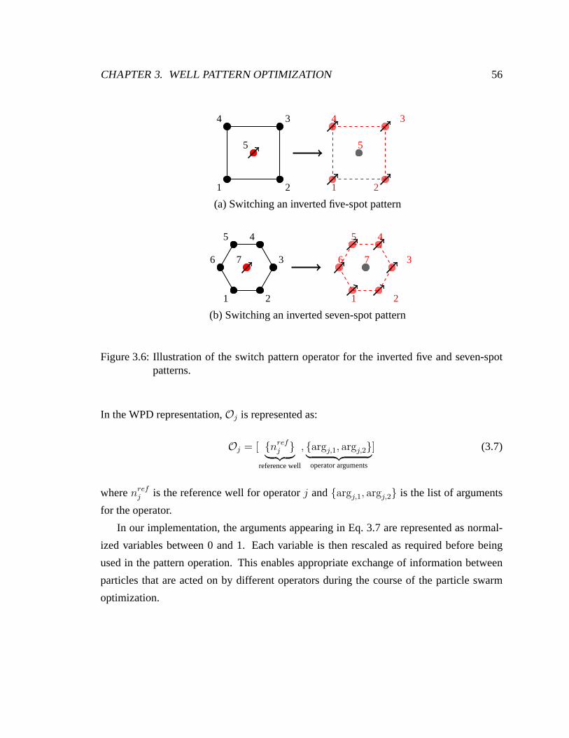
CHAPTER 3. WELL PATTERN OPTIMIZATION 56
1 2
34
5
1 2
34
5
(a) Switching an inverted five-spot pattern
1 2
3
45
6 7
1 2
3
45
6 7
(b) Switching an inverted seven-spot pattern
Figure 3.6: Illustration of the switch pattern operator forthe inverted five and seven-spotpatterns.
In the WPD representation,Oj is represented as:
Oj = [ {nrefj }
︸ ︷︷ ︸
reference well
, {argj,1, argj,2}︸ ︷︷ ︸
operator arguments
] (3.7)
wherenrefj is the reference well for operatorj and{argj,1, argj,2} is the list of arguments
for the operator.
In our implementation, the arguments appearing in Eq. 3.7 are represented as normal-
ized variables between 0 and 1. Each variable is then rescaled as required before being
used in the pattern operation. This enables appropriate exchange of information between
particles that are acted on by different operators during the course of the particle swarm
optimization.

CHAPTER 3. WELL PATTERN OPTIMIZATION 57
3.1.3 Solution Representation in WPD
We now describe the overall representation of potential solutions using the well pattern
description. Each solution (particle within our PSO implementation) consists of the ba-
sic well pattern definition and parameters (Eq. 3.1) and the representation for the pattern
operators (Eq. 3.7). In addition, each solution contains a set of variables that defines the
sequence of pattern operations when multiple operators areapplied. Theith PSO particle,
xi, is thus encoded as:
xi = [{Iwpi , [ξ0
i , η0
i , ai, bi]}︸ ︷︷ ︸
pattern parameters
{Si,1, Si,2, . . . , Si,No}
︸ ︷︷ ︸
operator sequence
{Oi,1,Oi,2, . . . ,Oi,No}
︸ ︷︷ ︸
pattern operators
], (3.8)
where{Iwpi , [ξ0
i , η0
i , ai, bi]} are the pattern parameters for particlei, No is the number of
pattern operators,{Oi,1,Oi,2, . . . ,Oi,No} provide the list of pattern operators, and
{Si,1, Si,2, . . . , Si,No} represent the sequence of application of the pattern operators. Each
Si,j, Si,j ∈ {0, 1, 2, . . . ,No}, is an integer variable representing the index of a pattern
operator. For example, ifSi,1 = 1 andSi,2 = 2, then the pattern operatorOi,1 is applied
first and pattern operatorOi,2 is applied second (using the well pattern generated from
Oi,1). If Si,j = 0, then thejth pattern operator (Oi,j) is skipped.
All components of any particlexi, which represents a PSO solution, are treated as real
numbers. However, some of the optimization parameters, such asnrefj andSi,j, are integers.
Where necessary, we determine integer values from real values by simply rounding to the
nearest integer.
Examples of using one pattern operator and two pattern operators in sequence are il-
lustrated in Figs. 3.7 and 3.8. In Fig. 3.7, the rotation operator is applied to the initial well
pattern (Fig. 3.7(a)) and the resulting pattern (Fig. 3.7(b)) is repeated over the entire do-
main (Fig. 3.7(c)). In the example in Fig. 3.8, the shear and scale operators are applied in
sequence to an inverted seven-spot pattern. As indicated above, wells that fall outside the
reservoir boundaries are eliminated. It is evident from these figures that a wide variety of
well patterns can be generated (and thus evaluated in the WPO procedure) using the WPD
representation.

CHAPTER 3. WELL PATTERN OPTIMIZATION 58
(a) Initial pattern (b) After rotation
(c) Repeated final pattern
Figure 3.7: Application of one pattern operator.
3.2 Well-by-Well Perturbation (WWP)
Optimization using WPD produces solutions that consist of repeated well patterns. It is
possible to further improve the solution by performing optimizations that involve perturb-
ing the well locations determined using WPD. We refer to this as well-by-well perturbation
(WWP). Following WWP, the basic patterns remain essentially intact, but the well locations
within the patterns are shifted to improve the objective function.
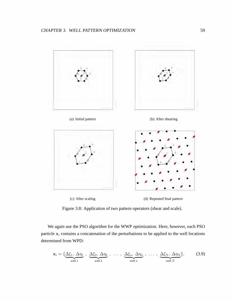
CHAPTER 3. WELL PATTERN OPTIMIZATION 59
(a) Initial pattern (b) After shearing
(c) After scaling (d) Repeated final pattern
Figure 3.8: Application of two pattern operators (shear andscale).
We again use the PSO algorithm for the WWP optimization. Here, however, each PSO
particlexi contains a concatenation of the perturbations to be appliedto the well locations
determined from WPD:
xi = {∆ξ1, ∆η1︸ ︷︷ ︸
well 1
, ∆ξ2, ∆η2︸ ︷︷ ︸
well 2
, . . . , ∆ξn, ∆ηn︸ ︷︷ ︸
well n
, . . . , ∆ξN , ∆ηN︸ ︷︷ ︸
well N
}, (3.9)
CHAPTER 3. WELL PATTERN OPTIMIZATION 60
whereN is the total number of wells as determined in the WPD optimization and∆ξn and
∆ηn represent the perturbations of the spatial locations of well n. Prior to simulation, the
actual well locations are obtained by adding the perturbations to the corresponding well lo-
cation from the WPD solution. In our implementation, the minimum and maximum values
of ∆ξn and∆ηn are constrained to keep wells from shifting from one patternto another.
We note that WWP could also be used for other determinations, such as the completion
interval for each well in three-dimensional problems. Elimination of wells could also be
considered through inclusion of an active/inactive optimization parameter for each well.
Neither of these options was considered in this work, thoughthey could be incorporated
easily into the WWP procedure (the dimension of the search space will, however, increase).
The WWP procedure introduces an efficient ‘local’ search, which leads to improved
solutions (as will be demonstrated below). Improved solutions are achieved because the
optimized well locations now account for local variations in porosity, permeability, and
other properties. The two procedures – WPD and WWP – are complementary because
WPD provides the ability to search efficiently on the large scale and to optimize well count,
while WWP enables local adjustments.
Although the dimension of the search space in WWP is the same as that using well-by-
well concatenation (for cases where the number of wells is specified), WWP has several
advantages over well-by-well concatenation. Specifically, in WWP, wells are allowed to
move only a limited number of grid blocks in each direction. This ‘constraint’ can be eas-
ily incorporated into the optimization, in contrast to the general well distance constraints
required using well-by-well concatenation. In addition, because wells can move only lo-
cally in WWP, the size of the search space is much smaller than that for well-by-well
concatenation (despite the fact that the dimension of the search space is the same in both
cases). Finally, in WWP the number of wells (as determined fromthe WPD optimization)
is fixed and does not need to be determined as part of the optimization. Using well-by-
well concatenation, however, the number of wells should also be an optimization variable,
which further complicates the optimization.
It is important to note that the use of WPD followed by WWP cannot be expected to
provide the overall global optimum that could (theoretically) be achieved through use of
well-by-well concatenation. This is because well-by-wellconcatenation entails a broader
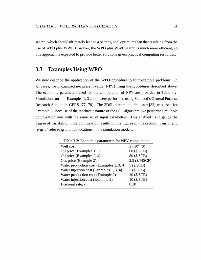
CHAPTER 3. WELL PATTERN OPTIMIZATION 61
search, which should ultimately lead to a better global optimum than that resulting from the
use of WPD plus WWP. However, the WPD plus WWP search is much more efficient, so
this approach is expected to provide better solutions givenpractical computing resources.
3.3 Examples Using WPO
We now describe the application of the WPO procedure to four example problems. In
all cases, we maximized net present value (NPV) using the procedures described above.
The economic parameters used for the computation of NPV are provided in Table 3.2.
Simulation runs for Examples 1, 3 and 4 were performed using Stanford’s General Purpose
Research Simulator, GPRS [77, 78]. The 3DSL streamline simulator [83] was used for
Example 2. Because of the stochastic nature of the PSO algorithm, we performed multiple
optimization runs with the same set of input parameters. This enabled us to gauge the
degree of variability in the optimization results. In the figures in this section, ‘x-grid’ and
‘y-grid’ refer to grid block locations in the simulation models.
Table 3.2: Economic parameters for NPV computation
Well cost 3×10⁶ ($)Oil price (Examples 1, 3) 60 ($/STB)Oil price (Examples 2, 4) 80 ($/STB)Gas price (Example 2) 2.5 ($/MSCF)Water production cost (Examples 1, 3, 4) 5 ($/STB)Water injection cost (Examples 1, 3, 4) 5 ($/STB)Water production cost (Example 2) 10 ($/STB)Water injection cost (Example 2) 10 ($/STB)Discount rate,r 0.10
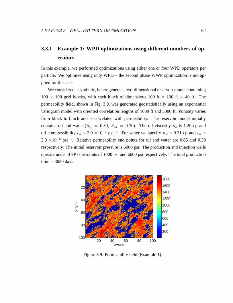
CHAPTER 3. WELL PATTERN OPTIMIZATION 62
3.3.1 Example 1: WPD optimizations using different numbers of op-
erators
In this example, we performed optimizations using either one or four WPD operators per
particle. We optimize using only WPD – the second phase WWP optimization is not ap-
plied for this case.
We considered a synthetic, heterogeneous, two-dimensional reservoir model containing
100 × 100 grid blocks, with each block of dimensions 100 ft× 100 ft × 40 ft. The
permeability field, shown in Fig. 3.9, was generated geostatistically using an exponential
variogram model with oriented correlation lengths of 1000 ft and 5000 ft. Porosity varies
from block to block and is correlated with permeability. Thereservoir model initially
contains oil and water (Soi = 0.80, Swi = 0.20). The oil viscosityµo is 1.20 cp and
oil compressibilityco is 2.0×10⁻⁵ psi−1. For water we specifyµw = 0.31 cp andcw =
2.9 ×10⁻⁶ psi−1. Relative permeability end points for oil and water are 0.85 and 0.30
respectively. The initial reservoir pressure is 5000 psi. The production and injection wells
operate under BHP constraints of 1000 psi and 6000 psi respectively. The total production
time is 3650 days.
x−grid
y−gr
id
20 40 60 80 100
20
40
60
80
100
200
400
600
800
1000
1200
1400
1600
1800
Figure 3.9: Permeability field (Example 1).
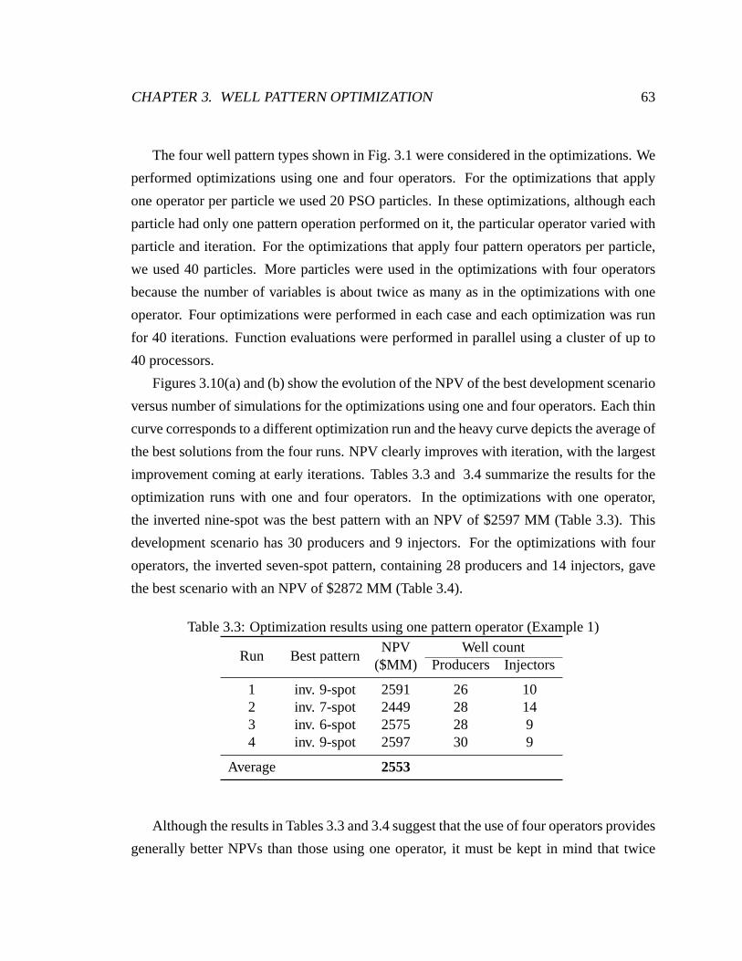
CHAPTER 3. WELL PATTERN OPTIMIZATION 63
The four well pattern types shown in Fig. 3.1 were consideredin the optimizations. We
performed optimizations using one and four operators. For the optimizations that apply
one operator per particle we used 20 PSO particles. In these optimizations, although each
particle had only one pattern operation performed on it, theparticular operator varied with
particle and iteration. For the optimizations that apply four pattern operators per particle,
we used 40 particles. More particles were used in the optimizations with four operators
because the number of variables is about twice as many as in the optimizations with one
operator. Four optimizations were performed in each case and each optimization was run
for 40 iterations. Function evaluations were performed in parallel using a cluster of up to
40 processors.
Figures 3.10(a) and (b) show the evolution of the NPV of the best development scenario
versus number of simulations for the optimizations using one and four operators. Each thin
curve corresponds to a different optimization run and the heavy curve depicts the average of
the best solutions from the four runs. NPV clearly improves with iteration, with the largest
improvement coming at early iterations. Tables 3.3 and 3.4 summarize the results for the
optimization runs with one and four operators. In the optimizations with one operator,
the inverted nine-spot was the best pattern with an NPV of $2597 MM (Table 3.3). This
development scenario has 30 producers and 9 injectors. For the optimizations with four
operators, the inverted seven-spot pattern, containing 28producers and 14 injectors, gave
the best scenario with an NPV of $2872 MM (Table 3.4).
Table 3.3: Optimization results using one pattern operator(Example 1)
Run Best patternNPV Well count
($MM) Producers Injectors
1 inv. 9-spot 2591 26 102 inv. 7-spot 2449 28 143 inv. 6-spot 2575 28 94 inv. 9-spot 2597 30 9
Average 2553
Although the results in Tables 3.3 and 3.4 suggest that the use of four operators provides
generally better NPVs than those using one operator, it mustbe kept in mind that twice
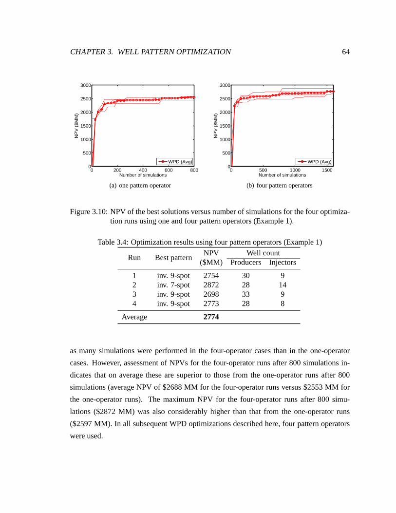
CHAPTER 3. WELL PATTERN OPTIMIZATION 64
0 200 400 600 8000
500
1000
1500
2000
2500
3000
NP
V (
$MM
)
Number of simulations
WPD (Avg)
(a) one pattern operator
0 500 1000 15000
500
1000
1500
2000
2500
3000
NP
V (
$MM
)
Number of simulations
WPD (Avg)
(b) four pattern operators
Figure 3.10: NPV of the best solutions versus number of simulations for the four optimiza-tion runs using one and four pattern operators (Example 1).
Table 3.4: Optimization results using four pattern operators (Example 1)
Run Best patternNPV Well count
($MM) Producers Injectors
1 inv. 9-spot 2754 30 92 inv. 7-spot 2872 28 143 inv. 9-spot 2698 33 94 inv. 9-spot 2773 28 8
Average 2774
as many simulations were performed in the four-operator cases than in the one-operator
cases. However, assessment of NPVs for the four-operator runs after 800 simulations in-
dicates that on average these are superior to those from the one-operator runs after 800
simulations (average NPV of $2688 MM for the four-operator runs versus $2553 MM for
the one-operator runs). The maximum NPV for the four-operator runs after 800 simu-
lations ($2872 MM) was also considerably higher than that from the one-operator runs
($2597 MM). In all subsequent WPD optimizations described here, four pattern operators
were used.
CHAPTER 3. WELL PATTERN OPTIMIZATION 65
Figures 3.11(a) and (b) show the well locations from the bestsolutions in the optimiza-
tions with one and four operators. The black dots inside white circles represent producer
wells while the black crosses inside white circles designate injection wells. In these figures,
the basic pattern element is depicted by the white lines. Theoil saturation at 500 days is
shown as background. It is evident that the best patterns are, in both cases, rotated with
respect to the reservoir boundaries. This results from the impact of reservoir heterogeneity
on the flow field. We note that, based on the oil saturation maps, both patterns appear to
provide efficient sweep. It is difficult to draw quantitativeconclusions from these maps,
however, as the pattern that appears to have more unswept oilat 500 days (Figure 3.11(b))
actually leads to a larger NPV over the full simulation.
x−grid
y−gr
id
20 40 60 80 100
20
40
60
80
100
0.2
0.3
0.4
0.5
0.6
0.7
(a) one pattern operator
x−grid
y−gr
id
20 40 60 80 100
20
40
60
80
100
0.2
0.3
0.4
0.5
0.6
0.7
(b) four pattern operators
Figure 3.11: Well locations of the best solutions using one operator and four operators (Ex-ample 1). Oil saturation at 500 days shown as background. Theblack dotsinside white circles represent producer wells while while the black crossesinside white circles designate injection wells.
We next compared the optimization results with those obtained using standard well
patterns (no optimization is performed). Results for standard patterns aligned with the
reservoir boundaries are presented in Table 3.5. We considered well patterns with spacings
from 20 acres to 50 acres. This range was determined based on the bounds specified fora
andb and for the pattern operator parameters. Results for standard patterns with 20 acre
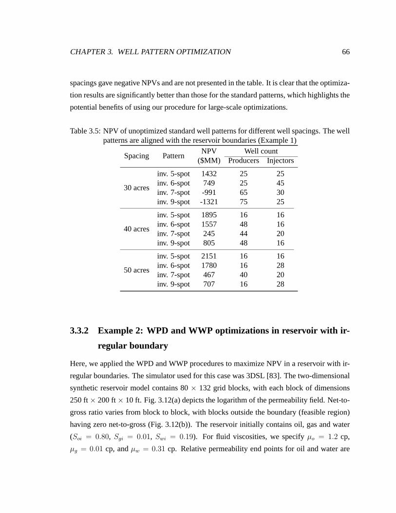
CHAPTER 3. WELL PATTERN OPTIMIZATION 66
spacings gave negative NPVs and are not presented in the table. It is clear that the optimiza-
tion results are significantly better than those for the standard patterns, which highlights the
potential benefits of using our procedure for large-scale optimizations.
Table 3.5: NPV of unoptimized standard well patterns for different well spacings. The wellpatterns are aligned with the reservoir boundaries (Example 1)
Spacing PatternNPV Well count
($MM) Producers Injectors
30 acres
inv. 5-spot 1432 25 25inv. 6-spot 749 25 45inv. 7-spot -991 65 30inv. 9-spot -1321 75 25
40 acres
inv. 5-spot 1895 16 16inv. 6-spot 1557 48 16inv. 7-spot 245 44 20inv. 9-spot 805 48 16
50 acres
inv. 5-spot 2151 16 16inv. 6-spot 1780 16 28inv. 7-spot 467 40 20inv. 9-spot 707 16 28
3.3.2 Example 2: WPD and WWP optimizations in reservoir with ir-
regular boundary
Here, we applied the WPD and WWP procedures to maximize NPV in a reservoir with ir-
regular boundaries. The simulator used for this case was 3DSL [83]. The two-dimensional
synthetic reservoir model contains 80× 132 grid blocks, with each block of dimensions
250 ft× 200 ft× 10 ft. Fig. 3.12(a) depicts the logarithm of the permeability field. Net-to-
gross ratio varies from block to block, with blocks outside the boundary (feasible region)
having zero net-to-gross (Fig. 3.12(b)). The reservoir initially contains oil, gas and water
(Soi = 0.80, Sgi = 0.01, Swi = 0.19). For fluid viscosities, we specifyµo = 1.2 cp,
µg = 0.01 cp, andµw = 0.31 cp. Relative permeability end points for oil and water are
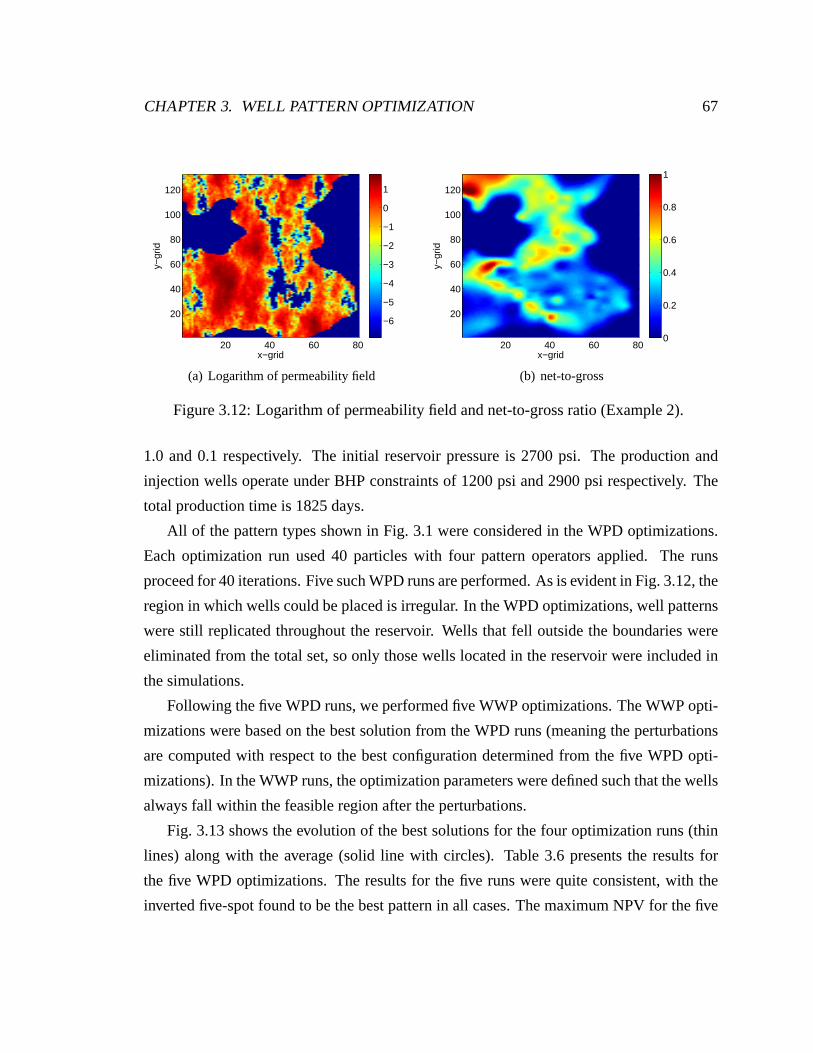
CHAPTER 3. WELL PATTERN OPTIMIZATION 67
x−grid
y−gr
id
20 40 60 80
20
40
60
80
100
120
−6
−5
−4
−3
−2
−1
0
1
(a) Logarithm of permeability field
x−grid
y−gr
id
20 40 60 80
20
40
60
80
100
120
0
0.2
0.4
0.6
0.8
1
(b) net-to-gross
Figure 3.12: Logarithm of permeability field and net-to-gross ratio (Example 2).
1.0 and 0.1 respectively. The initial reservoir pressure is2700 psi. The production and
injection wells operate under BHP constraints of 1200 psi and2900 psi respectively. The
total production time is 1825 days.
All of the pattern types shown in Fig. 3.1 were considered in the WPD optimizations.
Each optimization run used 40 particles with four pattern operators applied. The runs
proceed for 40 iterations. Five such WPD runs are performed. As is evident in Fig. 3.12, the
region in which wells could be placed is irregular. In the WPD optimizations, well patterns
were still replicated throughout the reservoir. Wells thatfell outside the boundaries were
eliminated from the total set, so only those wells located inthe reservoir were included in
the simulations.
Following the five WPD runs, we performed five WWP optimizations.The WWP opti-
mizations were based on the best solution from the WPD runs (meaning the perturbations
are computed with respect to the best configuration determined from the five WPD opti-
mizations). In the WWP runs, the optimization parameters weredefined such that the wells
always fall within the feasible region after the perturbations.
Fig. 3.13 shows the evolution of the best solutions for the four optimization runs (thin
lines) along with the average (solid line with circles). Table 3.6 presents the results for
the five WPD optimizations. The results for the five runs were quite consistent, with the
inverted five-spot found to be the best pattern in all cases. The maximum NPV for the five
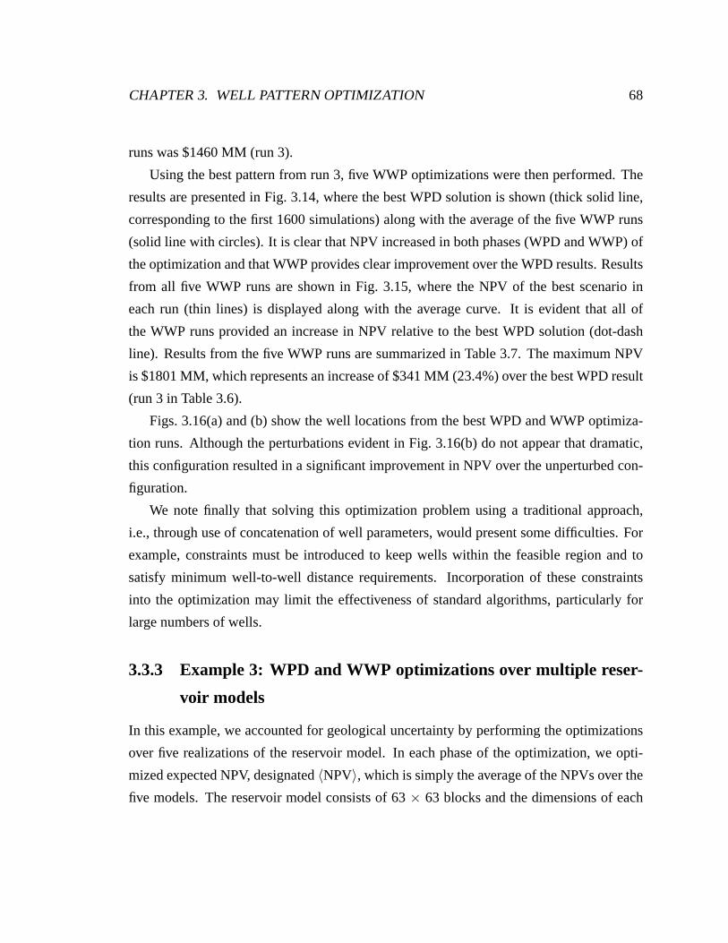
CHAPTER 3. WELL PATTERN OPTIMIZATION 68
runs was $1460 MM (run 3).
Using the best pattern from run 3, five WWP optimizations were then performed. The
results are presented in Fig. 3.14, where the best WPD solution is shown (thick solid line,
corresponding to the first 1600 simulations) along with the average of the five WWP runs
(solid line with circles). It is clear that NPV increased in both phases (WPD and WWP) of
the optimization and that WWP provides clear improvement overthe WPD results. Results
from all five WWP runs are shown in Fig. 3.15, where the NPV of the best scenario in
each run (thin lines) is displayed along with the average curve. It is evident that all of
the WWP runs provided an increase in NPV relative to the best WPD solution (dot-dash
line). Results from the five WWP runs are summarized in Table 3.7.The maximum NPV
is $1801 MM, which represents an increase of $341 MM (23.4%) over the best WPD result
(run 3 in Table 3.6).
Figs. 3.16(a) and (b) show the well locations from the best WPDand WWP optimiza-
tion runs. Although the perturbations evident in Fig. 3.16(b) do not appear that dramatic,
this configuration resulted in a significant improvement in NPV over the unperturbed con-
figuration.
We note finally that solving this optimization problem usinga traditional approach,
i.e., through use of concatenation of well parameters, would present some difficulties. For
example, constraints must be introduced to keep wells within the feasible region and to
satisfy minimum well-to-well distance requirements. Incorporation of these constraints
into the optimization may limit the effectiveness of standard algorithms, particularly for
large numbers of wells.
3.3.3 Example 3: WPD and WWP optimizations over multiple reser-
voir models
In this example, we accounted for geological uncertainty byperforming the optimizations
over five realizations of the reservoir model. In each phase of the optimization, we opti-
mized expected NPV, designated〈NPV〉, which is simply the average of the NPVs over the
five models. The reservoir model consists of 63× 63 blocks and the dimensions of each
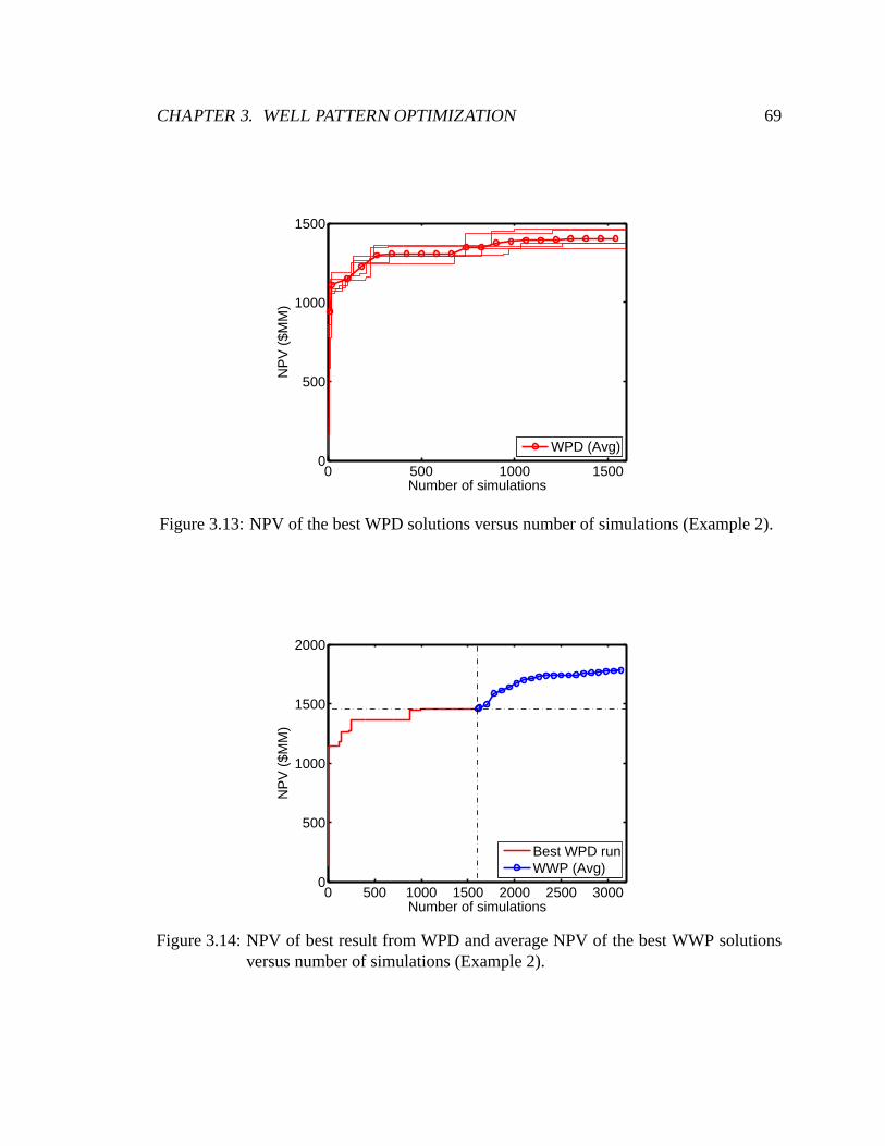
CHAPTER 3. WELL PATTERN OPTIMIZATION 69
0 500 1000 15000
500
1000
1500
Number of simulations
NP
V (
$MM
)
WPD (Avg)
Figure 3.13: NPV of the best WPD solutions versus number of simulations (Example 2).
0 500 1000 1500 2000 2500 30000
500
1000
1500
2000
Number of simulations
NP
V (
$MM
)
Best WPD runWWP (Avg)
Figure 3.14: NPV of best result from WPD and average NPV of the best WWP solutionsversus number of simulations (Example 2).
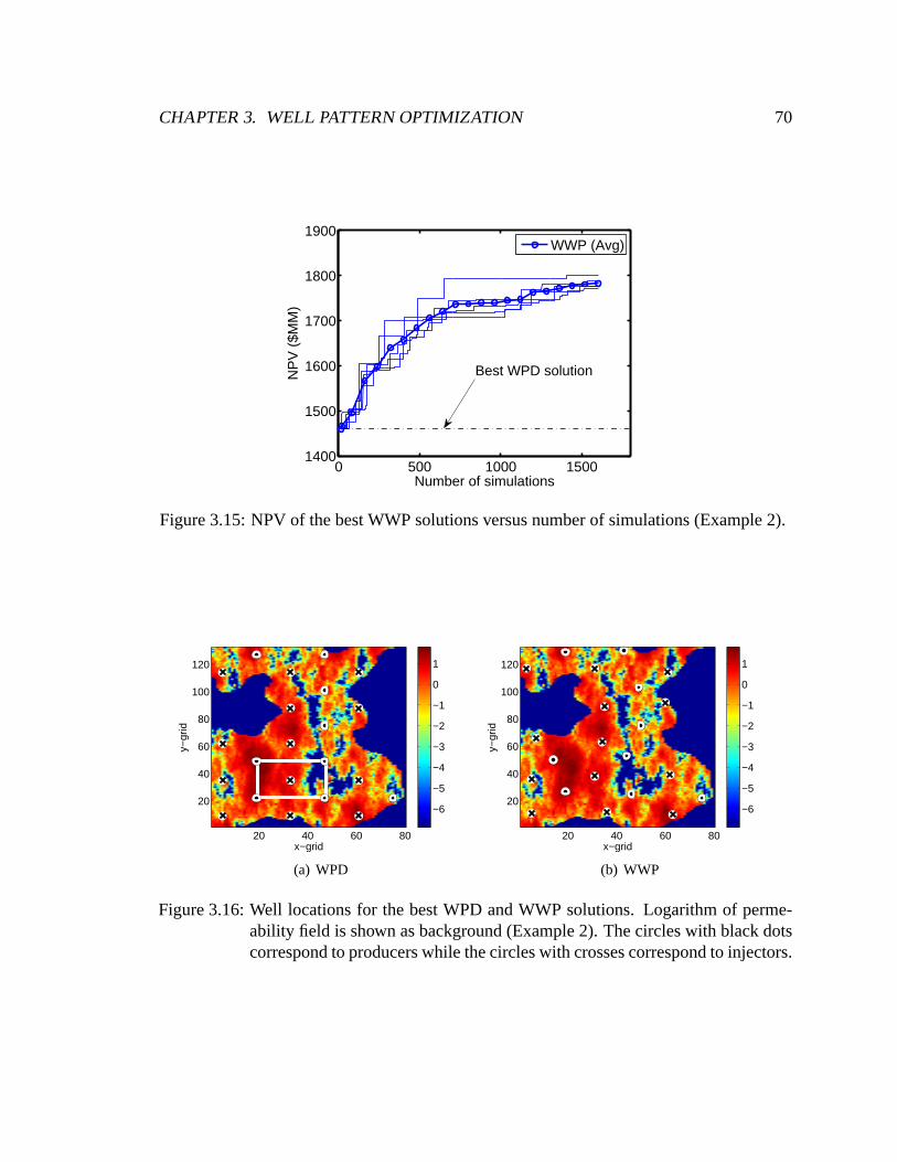
CHAPTER 3. WELL PATTERN OPTIMIZATION 70
0 500 1000 15001400
1500
1600
1700
1800
1900
Number of simulations
NP
V (
$MM
)
WWP (Avg)
Best WPD solution
Figure 3.15: NPV of the best WWP solutions versus number of simulations (Example 2).
x−grid
y−gr
id
20 40 60 80
20
40
60
80
100
120
−6
−5
−4
−3
−2
−1
0
1
(a) WPD
x−grid
y−gr
id
20 40 60 80
20
40
60
80
100
120
−6
−5
−4
−3
−2
−1
0
1
(b) WWP
Figure 3.16: Well locations for the best WPD and WWP solutions. Logarithm of perme-ability field is shown as background (Example 2). The circleswith black dotscorrespond to producers while the circles with crosses correspond to injectors.
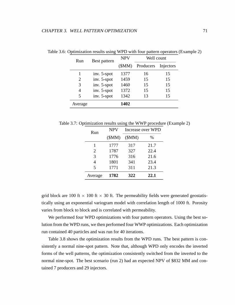
CHAPTER 3. WELL PATTERN OPTIMIZATION 71
Table 3.6: Optimization results using WPD with four pattern operators (Example 2)
Run Best patternNPV Well count
($MM) Producers Injectors
1 inv. 5-spot 1377 16 152 inv. 5-spot 1459 15 153 inv. 5-spot 1460 15 154 inv. 5-spot 1372 15 155 inv. 5-spot 1342 13 15
Average 1402
Table 3.7: Optimization results using the WWP procedure (Example 2)
RunNPV Increase over WPD
($MM) ($MM) %
1 1777 317 21.72 1787 327 22.43 1776 316 21.64 1801 341 23.45 1771 311 21.3
Average 1782 322 22.1
grid block are 100 ft× 100 ft× 30 ft. The permeability fields were generated geostatis-
tically using an exponential variogram model with correlation length of 1000 ft. Porosity
varies from block to block and is correlated with permeability.
We performed four WPD optimizations with four pattern operators. Using the best so-
lution from the WPD runs, we then performed four WWP optimizations. Each optimization
run contained 40 particles and was run for 40 iterations.
Table 3.8 shows the optimization results from the WPD runs. The best pattern is con-
sistently a normal nine-spot pattern. Note that, although WPD only encodes the inverted
forms of the well patterns, the optimization consistently switched from the inverted to the
normal nine-spot. The best scenario (run 2) had an expected NPV of $832 MM and con-
tained 7 producers and 29 injectors.
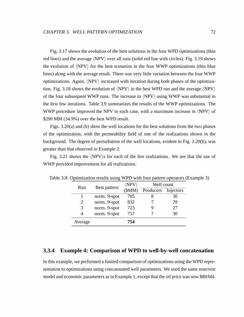
CHAPTER 3. WELL PATTERN OPTIMIZATION 72
Fig. 3.17 shows the evolution of the best solutions in the four WPD optimizations (thin
red lines) and the average〈NPV〉 over all runs (solid red line with circles). Fig. 3.19 shows
the evolution of〈NPV〉 for the best scenarios in the four WWP optimizations (thin blue
lines) along with the average result. There was very little variation between the four WWP
optimizations. Again,〈NPV〉 increased with iteration during both phases of the optimiza-
tion. Fig. 3.18 shows the evolution of〈NPV〉 in the best WPD run and the average〈NPV〉
of the four subsequent WWP runs. The increase in〈NPV〉 using WWP was substantial in
the first few iterations. Table 3.9 summarizes the results ofthe WWP optimizations. The
WWP procedure improved the NPV in each case, with a maximum increase in〈NPV〉 of
$290 MM (34.9%) over the best WPD result.
Figs. 3.20(a) and (b) show the well locations for the best solutions from the two phases
of the optimization, with the permeability field of one of therealizations shown in the
background. The degree of perturbation of the well locations, evident in Fig. 3.20(b), was
greater than that observed in Example 2.
Fig. 3.21 shows the〈NPV〉s for each of the five realizations. We see that the use of
WWP provided improvement for all realizations.
Table 3.8: Optimization results using WPD with four pattern operators (Example 3)
Run Best pattern〈NPV〉 Well count($MM) Producers Injectors
1 norm. 9-spot 705 8 302 norm. 9-spot 832 7 293 norm. 9-spot 723 9 274 norm. 9-spot 757 7 30
Average 754
3.3.4 Example 4: Comparison of WPD to well-by-well concatenation
In this example, we performed a limited comparison of optimizations using the WPD repre-
sentation to optimizations using concatenated well parameters. We used the same reservoir
model and economic parameters as in Example 1, except that the oil price was now $80/bbl.
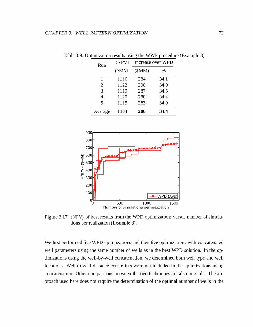
CHAPTER 3. WELL PATTERN OPTIMIZATION 73
Table 3.9: Optimization results using the WWP procedure (Example 3)
Run〈NPV〉 Increase over WPD
($MM) ($MM) %
1 1116 284 34.12 1122 290 34.93 1119 287 34.54 1120 288 34.45 1115 283 34.0
Average 1184 286 34.4
0 500 1000 15000
100
200
300
400
500
600
700
800
900
Number of simulations per realization
<N
PV
> (
$MM
)
WPD (Avg)
Figure 3.17:〈NPV〉 of best results from the WPD optimizations versus number of simula-tions per realization (Example 3).
We first performed five WPD optimizations and then five optimizations with concatenated
well parameters using the same number of wells as in the best WPD solution. In the op-
timizations using the well-by-well concatenation, we determined both well type and well
locations. Well-to-well distance constraints were not included in the optimizations using
concatenation. Other comparisons between the two techniques are also possible. The ap-
proach used here does not require the determination of the optimal number of wells in the
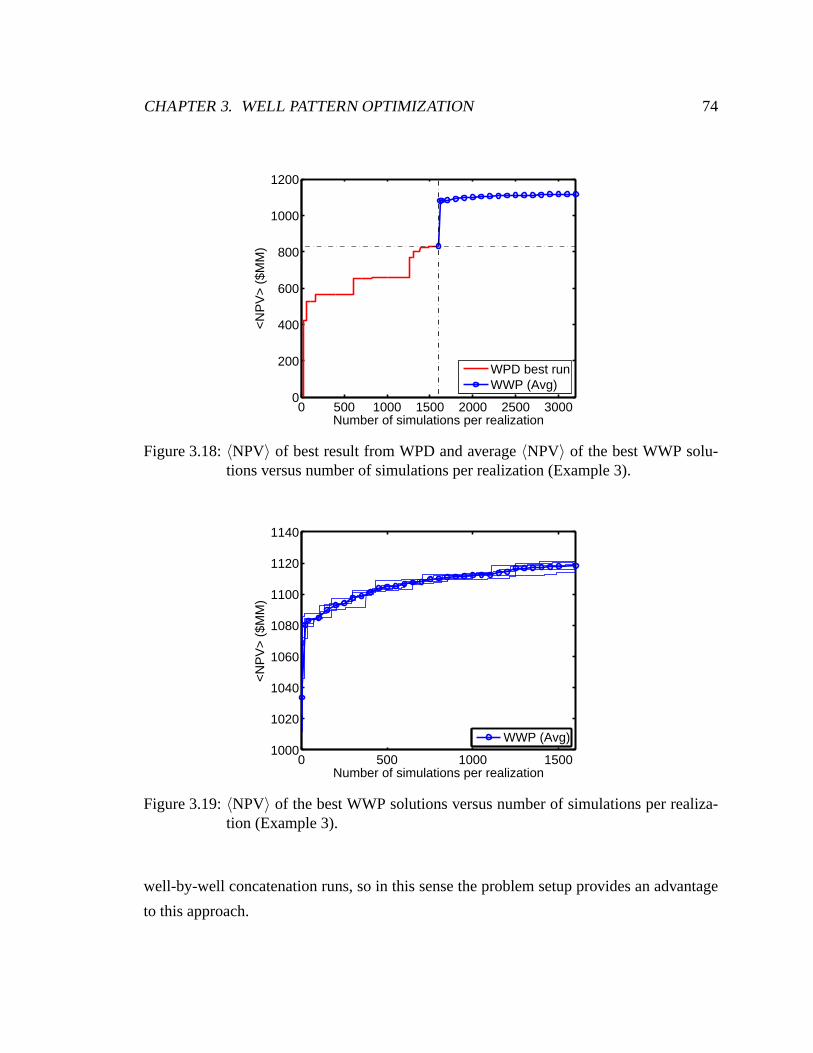
CHAPTER 3. WELL PATTERN OPTIMIZATION 74
0 500 1000 1500 2000 2500 30000
200
400
600
800
1000
1200
Number of simulations per realization
<N
PV
> (
$MM
)
WPD best runWWP (Avg)
Figure 3.18:〈NPV〉 of best result from WPD and average〈NPV〉 of the best WWP solu-tions versus number of simulations per realization (Example 3).
0 500 1000 15001000
1020
1040
1060
1080
1100
1120
1140
Number of simulations per realization
<N
PV
> (
$MM
)
WWP (Avg)
Figure 3.19:〈NPV〉 of the best WWP solutions versus number of simulations per realiza-tion (Example 3).
well-by-well concatenation runs, so in this sense the problem setup provides an advantage
to this approach.

CHAPTER 3. WELL PATTERN OPTIMIZATION 75
x−grid
y−gr
id
10 20 30 40 50 60
10
20
30
40
50
60
400
500
600
700
800
900
(a) WPD
x−grid
y−gr
id
10 20 30 40 50 60
10
20
30
40
50
60
400
500
600
700
800
900
(b) WWP
Figure 3.20: Well locations for the best WPD and WWP solutions. Permeability field forone of the realizations is shown as background (Example 3). The circles withblack dots correspond to producers while the circles with crosses correspondto injectors.
1 2 3 4 50
200
400
600
800
1000
1200
1400
1600
Realizations
NP
V (
$MM
)
WPDWPD+WWP
Figure 3.21: NPV of the phase 1 (WPD) and phase 2 (WWP) optimizations for each real-ization (Example 3).
In all optimizations, we used the PSO algorithm with 30 particles. Each optimization
was run for 15 iterations. Fig. 3.22 shows the evolution of the average NPV of the best
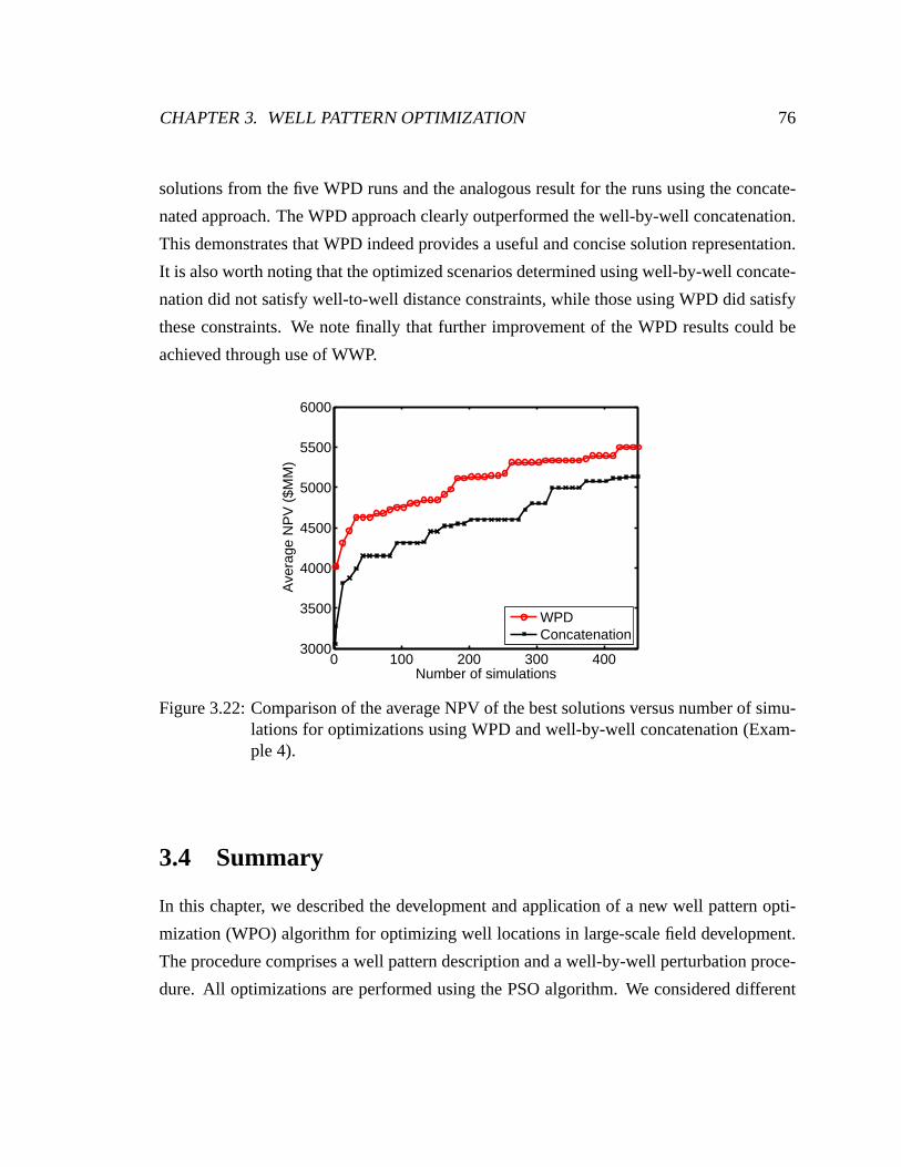
CHAPTER 3. WELL PATTERN OPTIMIZATION 76
solutions from the five WPD runs and the analogous result for the runs using the concate-
nated approach. The WPD approach clearly outperformed the well-by-well concatenation.
This demonstrates that WPD indeed provides a useful and concise solution representation.
It is also worth noting that the optimized scenarios determined using well-by-well concate-
nation did not satisfy well-to-well distance constraints,while those using WPD did satisfy
these constraints. We note finally that further improvementof the WPD results could be
achieved through use of WWP.
0 100 200 300 4003000
3500
4000
4500
5000
5500
6000
Number of simulations
Ave
rage
NP
V (
$MM
)
WPDConcatenation
Figure 3.22: Comparison of the average NPV of the best solutions versus number of simu-lations for optimizations using WPD and well-by-well concatenation (Exam-ple 4).
3.4 Summary
In this chapter, we described the development and application of a new well pattern opti-
mization (WPO) algorithm for optimizing well locations in large-scale field development.
The procedure comprises a well pattern description and a well-by-well perturbation proce-
dure. All optimizations are performed using the PSO algorithm. We considered different
CHAPTER 3. WELL PATTERN OPTIMIZATION 77
optimization problems and different variants of the WPO procedure. In the examples con-
sidered, the WPD procedure provided significant increases inNPV, and further improve-
ments are possible using the WWP technique. These examples demonstrate the applicabil-
ity of the WPO procedure for optimization problems with many wells.
In the WPO optimizations, we have used default PSO parameters(ω, c1, c2) and the
random variable neighborhood topology described in Chapter2. Better optimization re-
sults may be obtained by tuning the PSO parameters. In the next chapter, we describe the
application of a metaoptimization procedure for optimizing PSO parameters in the WPO
optimizations.

Chapter 4
Metaoptimization for PSO Parameter
Determination
In this chapter, we describe the implementation of metaoptimization techniques to deter-
mine optimal PSO parameters. First, we describe the metaoptimization procedure. We ap-
plied this approach to determine appropriate parameter values by considering four bench-
mark well placement optimization problems. The optimized PSO parameters were then
used for two realistic well placement optimization problems including optimizing the loca-
tion of 15 vertical wells and WPD optimizations in two-dimensional reservoir models. For
these problems, we performed several optimizations using default and optimized param-
eters. We also applied the metaoptimization procedure directly to the target optimization
problems (i.e., the optimal parameters are determined for the actual problem, not the bench-
mark problems). The results in this chapter demonstrate theeffectiveness of the metaopti-
mization procedure.
4.1 PSO Metaoptimization
In Chapters 2 and 3 we applied the PSO algorithm for well placement optimization, using
PSO parameters taken from the literature. As is the case for other stochastic optimization
algorithms, the performance of PSO depends on the values assigned to the algorithm pa-
rameters. In this chapter, we describe the application of a metaoptimization procedure to
78
CHAPTER 4. METAOPTIMIZATION FOR PARAMETER DETERMINATION 79
optimize the key PSO parameters directly.
In PSO metaoptimization, two PSO algorithms are used [2, 69]. The first PSO algo-
rithm optimizes PSO parameters, while the second PSO algorithm uses the optimized pa-
rameters to solve a specified optimization problem or problems. The first and second PSO
algorithms are referred to as the “superswarm PSO” and “subswarm PSO” respectively
[69]. The metaoptimization procedure can be used to determine optimal PSO parameter
values for a set of small benchmark problems or it can be directly applied to the target
optimization problem. In the former case, the assumption isthat the parameters that are
optimal for the benchmark problems are also appropriate forother problems. We consider
both approaches in this chapter.
The metaoptimization procedure consists of three components: superswarm PSO, sub-
swarm PSO, and one or more optimization problems (optimizedby the subswarm PSO).
Each superswarm particle has associated PSO subswarms. Several subswarm optimiza-
tions are performed in order to evaluate the objective function value of a superswarm par-
ticle. The relationship between the superswarm and subswarm PSO algorithms is shown in
Fig. 4.1. In the figure,N designates the number of subswarm particles andT the number
of subswarm iterations. We now describe the superswarm and subswarm PSO procedures.
4.1.1 Superswarm PSO
The superswarm PSO optimizes the parameters required by thePSO algorithm. As shown
in Eq. 2.2, repeated here for completeness, some of these parameters (ω, c1, c2) are used in
the computation of PSO particle velocity,vi(k + 1):
vi(k + 1) = ω · vi(k)
+ c1 · D1(k) · (xpbesti (k) − xi(k))
+ c2 · D2(k) · (xnbesti (k) − xi(k)),
(4.1)
whereω, c1 andc2 are the weights of the inertia, cognitive, and social components;D1(k)
andD2(k) are diagonal matrices whose diagonal components are uniformly distributed
random variables in the range [0, 1];xi(k) is the position of theith particle at iteration
k; xpbesti (k) is the previous best particle position, andx
nbesti (k) is the best position in the
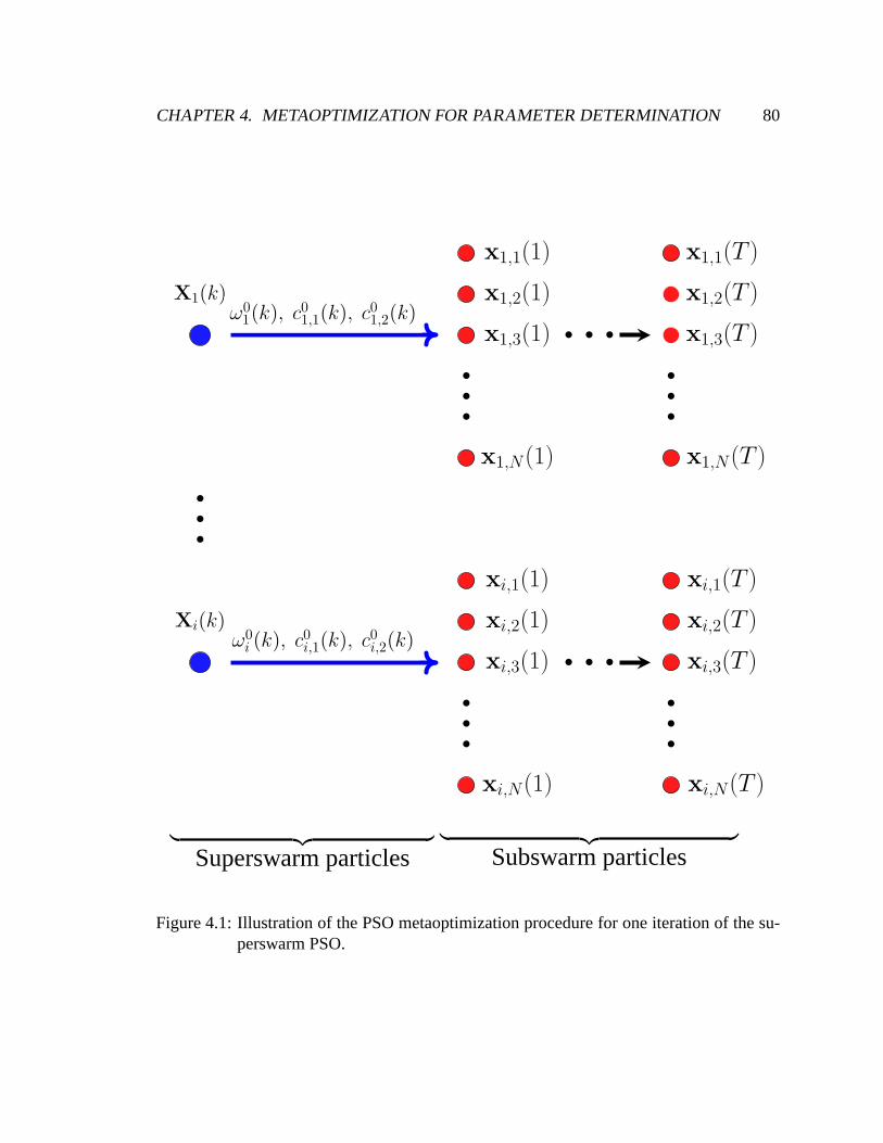
CHAPTER 4. METAOPTIMIZATION FOR PARAMETER DETERMINATION 80
X1(k)ω0
1(k), c01,1(k), c0
1,2(k)
x1,1(1)
x1,2(1)
x1,3(1)
•••
x1,N(1)
• • •
x1,1(T )
x1,2(T )
x1,3(T )
•••
x1,N(T )
•••
Xi(k)ω0
i (k), c0i,1(k), c0
i,2(k)
xi,1(1)
xi,2(1)
xi,3(1)
•••
xi,N(1)
• • •
xi,1(T )
xi,2(T )
xi,3(T )
•••
xi,N(T )
JeromeOnwunaluIsHereand︸ ︷︷ ︸
Superswarm particlesJeromeOnwunaluIsHereandand︸ ︷︷ ︸
Subswarm particles
Figure 4.1: Illustration of the PSO metaoptimization procedure for one iteration of the su-perswarm PSO.
CHAPTER 4. METAOPTIMIZATION FOR PARAMETER DETERMINATION 81
neighborhood of particlei. In addition to these parameters, we can also optimize the neigh-
borhood topology type (ntype). The topology determines howxnbest is determined. In our
optimizations, we will consider four different neighborhood topologies including the star,
ring, cluster and random variable topologies. These topologies are described in Section
2.1.1.
The superswarm PSO seeks to minimize average error (if the global optimum is known)
or maximize the average objective function values from several subswarm PSO optimiza-
tions. Multiple subswarm optimizations are performed (using the same PSO parameters)
because of the stochastic nature of the PSO algorithm.
Each superswarm particle represents the set of PSO parameters to be optimized. The
definition of the objective function of each superswarm particle depends on the number of
test optimization problems considered and on the number of repetitions of the subswarm
optimizations. We now describe the objective function evaluation for the superswarm PSO
where we seek to determine optimal parameter values forω, c1, c2 andntype. Let p, p ∈
{1, 2, . . . , P} be the index of a test optimization problem. LetXi(k) be the position of the
ith superswarm particle at iterationk and letep,r denote the best solution obtained from run
r of a subswarm optimization using test problemp. The objective function value of theith
particle,Fi(Xi(k)), is computed as follows:
Fi(Xi(k)) =1
P
P∑
p=1
1
R
R∑
r=1
ep,r , (4.2)
whereP is the number of test optimization problems considered andR is the number of
repetitions of the subswarm optimizations. In our applications we used values ofp from 1
to 4 and for the metaoptimizations using benchmark problemswe specifiedR = 20.
4.1.2 Subswarm PSO
The subswarm PSO optimizes the test problem(s) using the parameters from the associated
superswarm particle. Letxi,j(t) denote the position of thejth subswarm associated with
theith superswarm particle,Xi(k) (see Fig. 4.1). In each iteration of the superswarm PSO,
evaluation of the objective function for each superswarm particle requires one or more
CHAPTER 4. METAOPTIMIZATION FOR PARAMETER DETERMINATION 82
subswarm optimizations. For each subswarm PSO, the PSO parameters are fixed. In the
subswarm PSO, the particle velocity,vi,j(t + 1), is computed as follows:
vi,j(t + 1) = ω0
i (k) · vi,j(t)
+ c0
i,1(k) · D1(t) · (xpbesti,j (t) − xi,j(t))
+ c0
i,2(k) · D2(t) · (xnbesti,j (t) − xi,j(t)),
(4.3)
wheret is the index of subswarm iteration andω0
i (k), c0
i,1(k) andc0
i,2(k) are the parameter
values from superswarm particleXi(k). The objective function of a subswarm particle
depends on the optimization problem to be solved. If the global optimum is known, then the
subswarm PSO seeks to minimize error. Otherwise, the fitnessof the actual optimization
problem is maximized (or minimized). The overall flow chart of the metaoptimization
procedure is shown in Fig. 4.2.
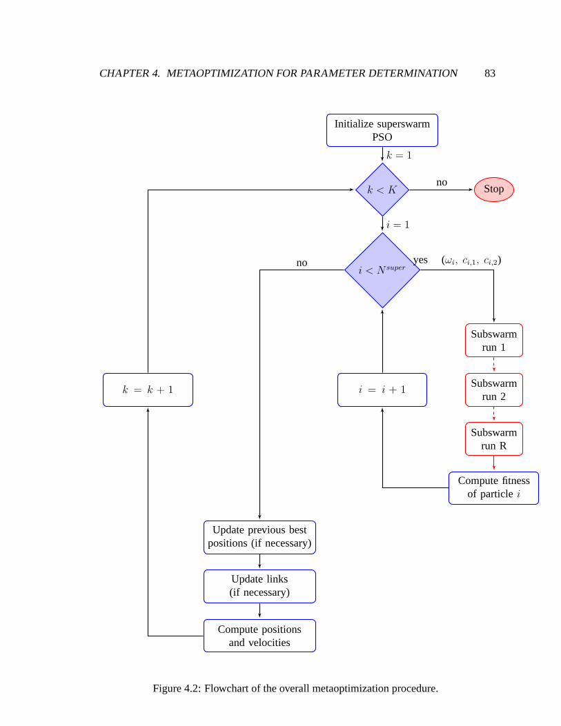
CHAPTER 4. METAOPTIMIZATION FOR PARAMETER DETERMINATION 83
Initialize superswarmPSO
k < K Stop
i < N super
Subswarmrun 1
k = k + 1 i = i + 1Subswarm
run 2
Subswarmrun R
Compute fitnessof particle i
Update previous bestpositions (if necessary)
Update links(if necessary)
Compute positionsand velocities
k = 1
no
i = 1
yes (ωi, ci,1, ci,2)no
Figure 4.2: Flowchart of the overall metaoptimization procedure.
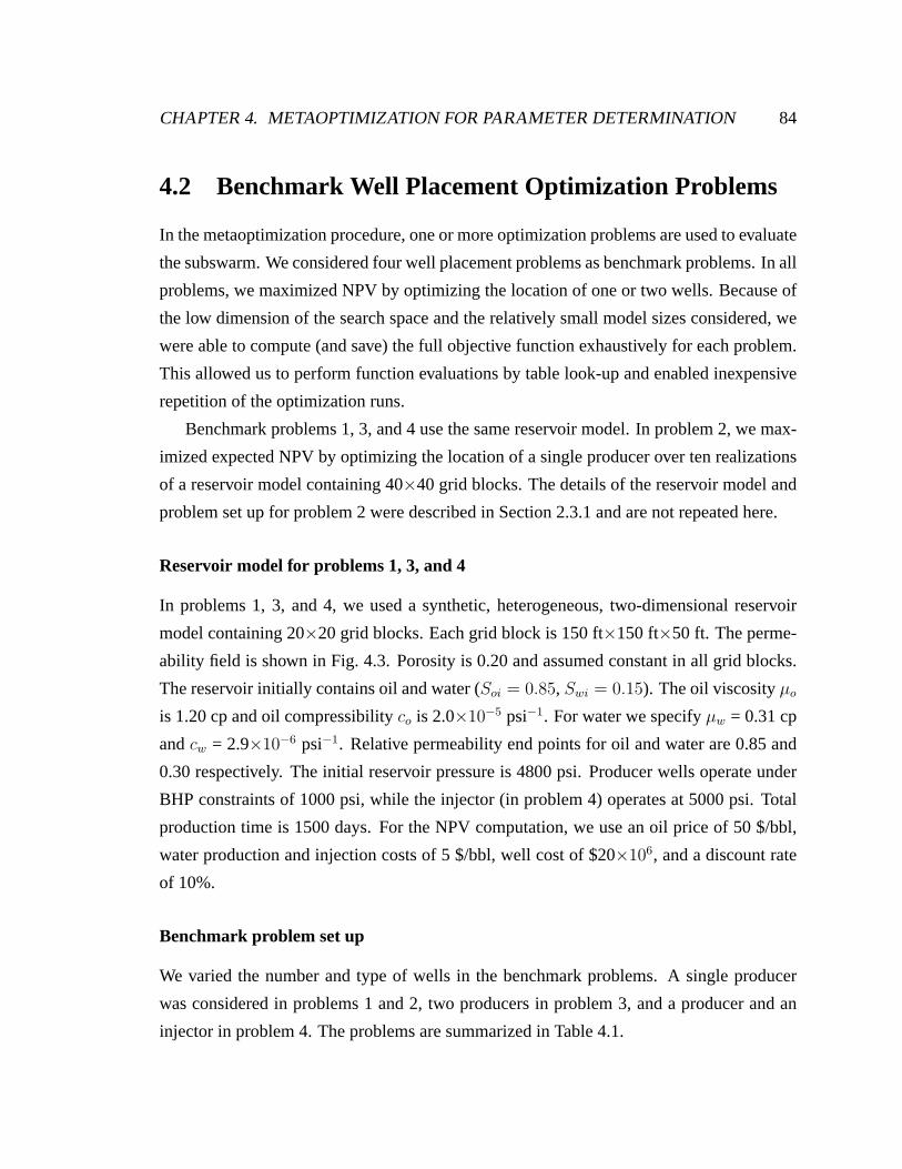
CHAPTER 4. METAOPTIMIZATION FOR PARAMETER DETERMINATION 84
4.2 Benchmark Well Placement Optimization Problems
In the metaoptimization procedure, one or more optimization problems are used to evaluate
the subswarm. We considered four well placement problems asbenchmark problems. In all
problems, we maximized NPV by optimizing the location of oneor two wells. Because of
the low dimension of the search space and the relatively small model sizes considered, we
were able to compute (and save) the full objective function exhaustively for each problem.
This allowed us to perform function evaluations by table look-up and enabled inexpensive
repetition of the optimization runs.
Benchmark problems 1, 3, and 4 use the same reservoir model. Inproblem 2, we max-
imized expected NPV by optimizing the location of a single producer over ten realizations
of a reservoir model containing 40×40 grid blocks. The details of the reservoir model and
problem set up for problem 2 were described in Section 2.3.1 and are not repeated here.
Reservoir model for problems 1, 3, and 4
In problems 1, 3, and 4, we used a synthetic, heterogeneous, two-dimensional reservoir
model containing 20×20 grid blocks. Each grid block is 150 ft×150 ft×50 ft. The perme-
ability field is shown in Fig. 4.3. Porosity is 0.20 and assumed constant in all grid blocks.
The reservoir initially contains oil and water (Soi = 0.85, Swi = 0.15). The oil viscosityµo
is 1.20 cp and oil compressibilityco is 2.0×10⁻⁵ psi−1. For water we specifyµw = 0.31 cp
andcw = 2.9×10⁻⁶ psi−1. Relative permeability end points for oil and water are 0.85 and
0.30 respectively. The initial reservoir pressure is 4800 psi. Producer wells operate under
BHP constraints of 1000 psi, while the injector (in problem 4)operates at 5000 psi. Total
production time is 1500 days. For the NPV computation, we usean oil price of 50 $/bbl,
water production and injection costs of 5 $/bbl, well cost of$20×106, and a discount rate
of 10%.
Benchmark problem set up
We varied the number and type of wells in the benchmark problems. A single producer
was considered in problems 1 and 2, two producers in problem 3, and a producer and an
injector in problem 4. The problems are summarized in Table 4.1.
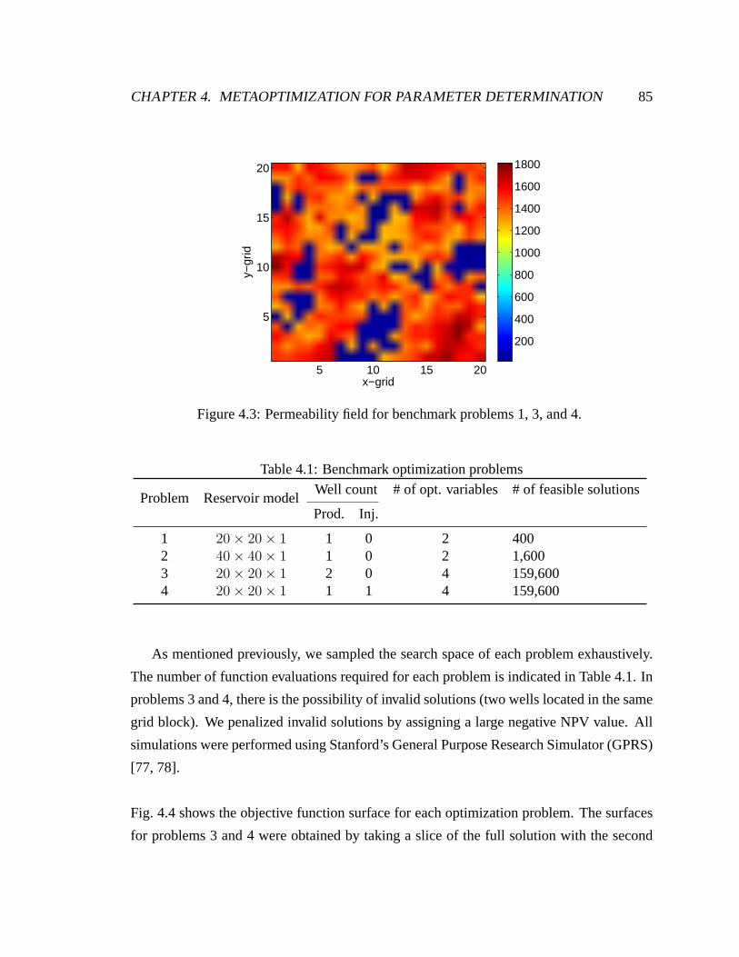
CHAPTER 4. METAOPTIMIZATION FOR PARAMETER DETERMINATION 85
x−grid
y−gr
id
5 10 15 20
5
10
15
20
200
400
600
800
1000
1200
1400
1600
1800
Figure 4.3: Permeability field for benchmark problems 1, 3, and 4.
Table 4.1: Benchmark optimization problems
Problem Reservoir modelWell count # of opt. variables # of feasible solutions
Prod. Inj.
1 20 × 20 × 1 1 0 2 4002 40 × 40 × 1 1 0 2 1,6003 20 × 20 × 1 2 0 4 159,6004 20 × 20 × 1 1 1 4 159,600
As mentioned previously, we sampled the search space of eachproblem exhaustively.
The number of function evaluations required for each problem is indicated in Table 4.1. In
problems 3 and 4, there is the possibility of invalid solutions (two wells located in the same
grid block). We penalized invalid solutions by assigning a large negative NPV value. All
simulations were performed using Stanford’s General Purpose Research Simulator (GPRS)
[77, 78].
Fig. 4.4 shows the objective function surface for each optimization problem. The surfaces
for problems 3 and 4 were obtained by taking a slice of the fullsolution with the second
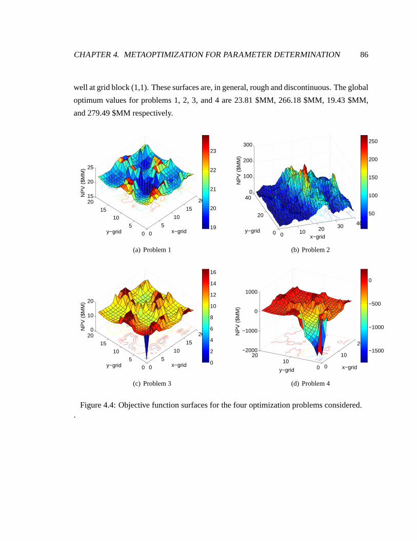
CHAPTER 4. METAOPTIMIZATION FOR PARAMETER DETERMINATION 86
well at grid block (1,1). These surfaces are, in general, rough and discontinuous. The global
optimum values for problems 1, 2, 3, and 4 are 23.81 $MM, 266.18 $MM, 19.43 $MM,
and 279.49 $MM respectively.
0
5
10
15
20
0
5
10
15
2015
20
25
x−gridy−grid
NP
V (
$MM
)
19
20
21
22
23
(a) Problem 1
0 10 20 30 40
0
20
400
100
200
300
x−gridy−grid
NP
V (
$MM
)
50
100
150
200
250
(b) Problem 2
0
5
10
15
20
0
5
10
15
200
10
20
x−gridy−grid
NP
V (
$MM
)
0
2
4
6
8
10
12
14
16
(c) Problem 3
0
10
20
010
20−2000
−1000
0
1000
x−gridy−grid
NP
V (
$MM
)
−1500
−1000
−500
0
(d) Problem 4
Figure 4.4: Objective function surfaces for the four optimization problems considered..
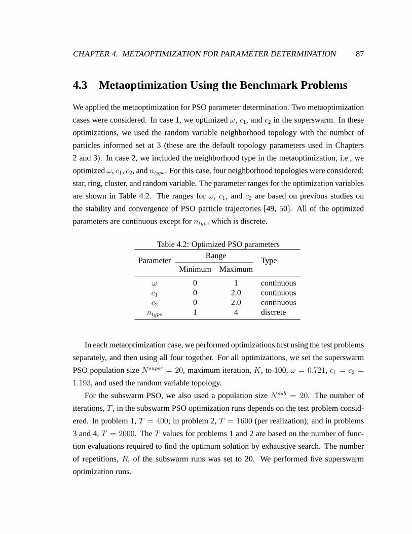
CHAPTER 4. METAOPTIMIZATION FOR PARAMETER DETERMINATION 87
4.3 Metaoptimization Using the Benchmark Problems
We applied the metaoptimization for PSO parameter determination. Two metaoptimization
cases were considered. In case 1, we optimizedω, c1, andc2 in the superswarm. In these
optimizations, we used the random variable neighborhood topology with the number of
particles informed set at 3 (these are the default topology parameters used in Chapters
2 and 3). In case 2, we included the neighborhood type in the metaoptimization, i.e., we
optimizedω, c1, c2, andntype. For this case, four neighborhood topologies were considered:
star, ring, cluster, and random variable. The parameter ranges for the optimization variables
are shown in Table 4.2. The ranges forω, c1, andc2 are based on previous studies on
the stability and convergence of PSO particle trajectories[49, 50]. All of the optimized
parameters are continuous except forntype which is discrete.
Table 4.2: Optimized PSO parameters
ParameterRange
TypeMinimum Maximum
ω 0 1 continuousc1 0 2.0 continuousc2 0 2.0 continuous
ntype 1 4 discrete
In each metaoptimization case, we performed optimizationsfirst using the test problems
separately, and then using all four together. For all optimizations, we set the superswarm
PSO population sizeN super = 20, maximum iteration,K, to 100,ω = 0.721, c1 = c2 =
1.193, and used the random variable topology.
For the subswarm PSO, we also used a population sizeN sub = 20. The number of
iterations,T , in the subswarm PSO optimization runs depends on the test problem consid-
ered. In problem 1,T = 400; in problem 2,T = 1600 (per realization); and in problems
3 and 4,T = 2000. TheT values for problems 1 and 2 are based on the number of func-
tion evaluations required to find the optimum solution by exhaustive search. The number
of repetitions,R, of the subswarm runs was set to 20. We performed five superswarm
optimization runs.
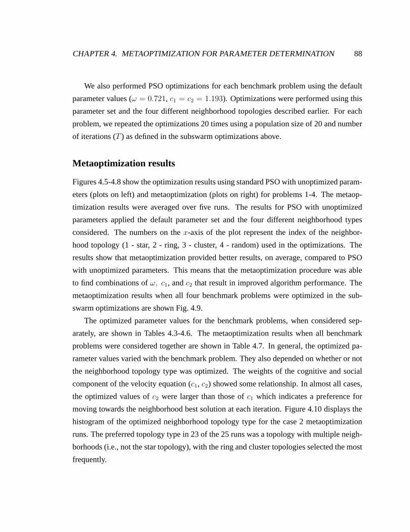
CHAPTER 4. METAOPTIMIZATION FOR PARAMETER DETERMINATION 88
We also performed PSO optimizations for each benchmark problem using the default
parameter values (ω = 0.721, c1 = c2 = 1.193). Optimizations were performed using this
parameter set and the four different neighborhood topologies described earlier. For each
problem, we repeated the optimizations 20 times using a population size of 20 and number
of iterations (T ) as defined in the subswarm optimizations above.
Metaoptimization results
Figures 4.5-4.8 show the optimization results using standard PSO with unoptimized param-
eters (plots on left) and metaoptimization (plots on right)for problems 1-4. The metaop-
timization results were averaged over five runs. The resultsfor PSO with unoptimized
parameters applied the default parameter set and the four different neighborhood types
considered. The numbers on thex-axis of the plot represent the index of the neighbor-
hood topology (1 - star, 2 - ring, 3 - cluster, 4 - random) used in the optimizations. The
results show that metaoptimization provided better results, on average, compared to PSO
with unoptimized parameters. This means that the metaoptimization procedure was able
to find combinations ofω, c1, andc2 that result in improved algorithm performance. The
metaoptimization results when all four benchmark problemswere optimized in the sub-
swarm optimizations are shown Fig. 4.9.
The optimized parameter values for the benchmark problems,when considered sep-
arately, are shown in Tables 4.3-4.6. The metaoptimizationresults when all benchmark
problems were considered together are shown in Table 4.7. Ingeneral, the optimized pa-
rameter values varied with the benchmark problem. They alsodepended on whether or not
the neighborhood topology type was optimized. The weights of the cognitive and social
component of the velocity equation (c1, c2) showed some relationship. In almost all cases,
the optimized values ofc2 were larger than those ofc1 which indicates a preference for
moving towards the neighborhood best solution at each iteration. Figure 4.10 displays the
histogram of the optimized neighborhood topology type for the case 2 metaoptimization
runs. The preferred topology type in 23 of the 25 runs was a topology with multiple neigh-
borhoods (i.e., not the star topology), with the ring and cluster topologies selected the most
frequently.
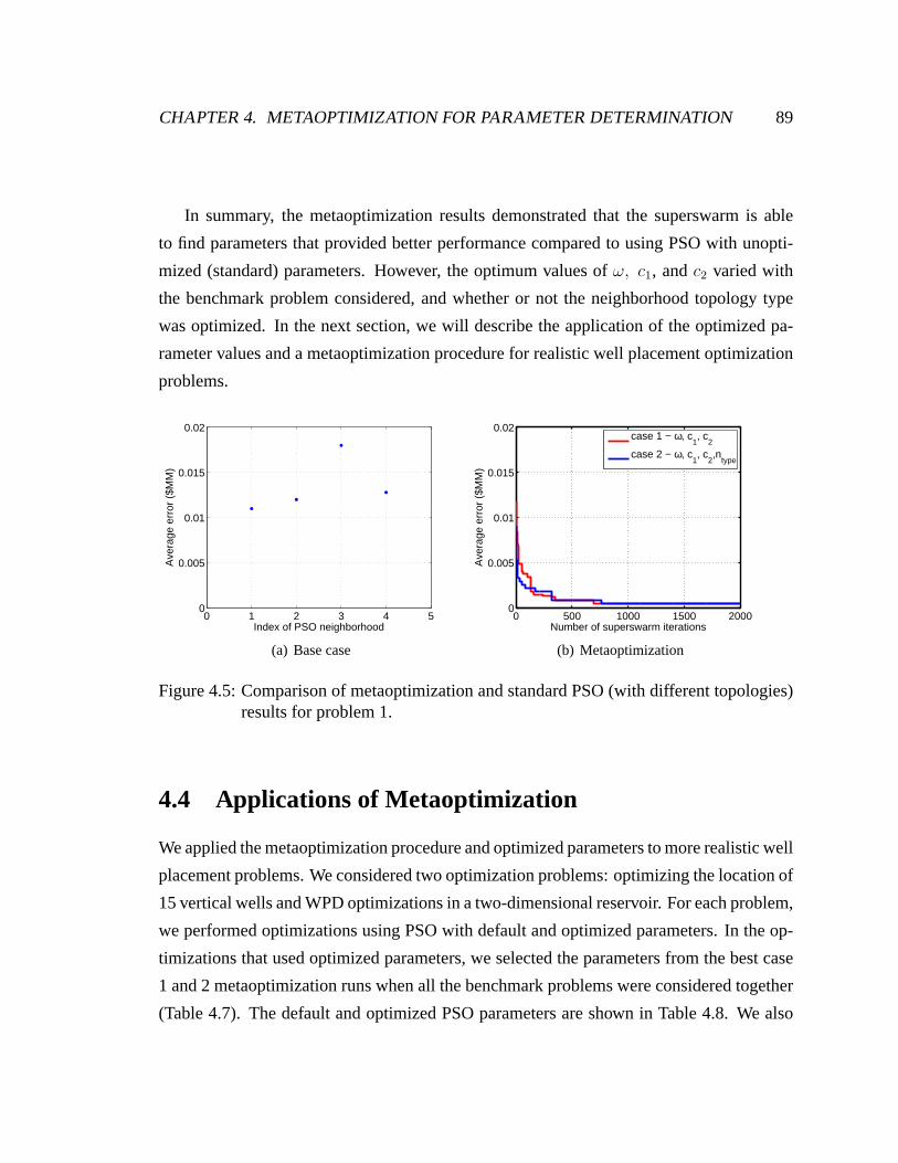
CHAPTER 4. METAOPTIMIZATION FOR PARAMETER DETERMINATION 89
In summary, the metaoptimization results demonstrated that the superswarm is able
to find parameters that provided better performance compared to using PSO with unopti-
mized (standard) parameters. However, the optimum values of ω, c1, andc2 varied with
the benchmark problem considered, and whether or not the neighborhood topology type
was optimized. In the next section, we will describe the application of the optimized pa-
rameter values and a metaoptimization procedure for realistic well placement optimization
problems.
0 1 2 3 4 50
0.005
0.01
0.015
0.02
Index of PSO neighborhood
Ave
rage
err
or (
$MM
)
(a) Base case
0 500 1000 1500 20000
0.005
0.01
0.015
0.02
Number of superswarm iterations
Ave
rage
err
or (
$MM
)
case 1 − ω, c1, c
2
case 2 − ω, c1, c
2,n
type
(b) Metaoptimization
Figure 4.5: Comparison of metaoptimization and standard PSO(with different topologies)results for problem 1.
4.4 Applications of Metaoptimization
We applied the metaoptimization procedure and optimized parameters to more realistic well
placement problems. We considered two optimization problems: optimizing the location of
15 vertical wells and WPD optimizations in a two-dimensionalreservoir. For each problem,
we performed optimizations using PSO with default and optimized parameters. In the op-
timizations that used optimized parameters, we selected the parameters from the best case
1 and 2 metaoptimization runs when all the benchmark problems were considered together
(Table 4.7). The default and optimized PSO parameters are shown in Table 4.8. We also
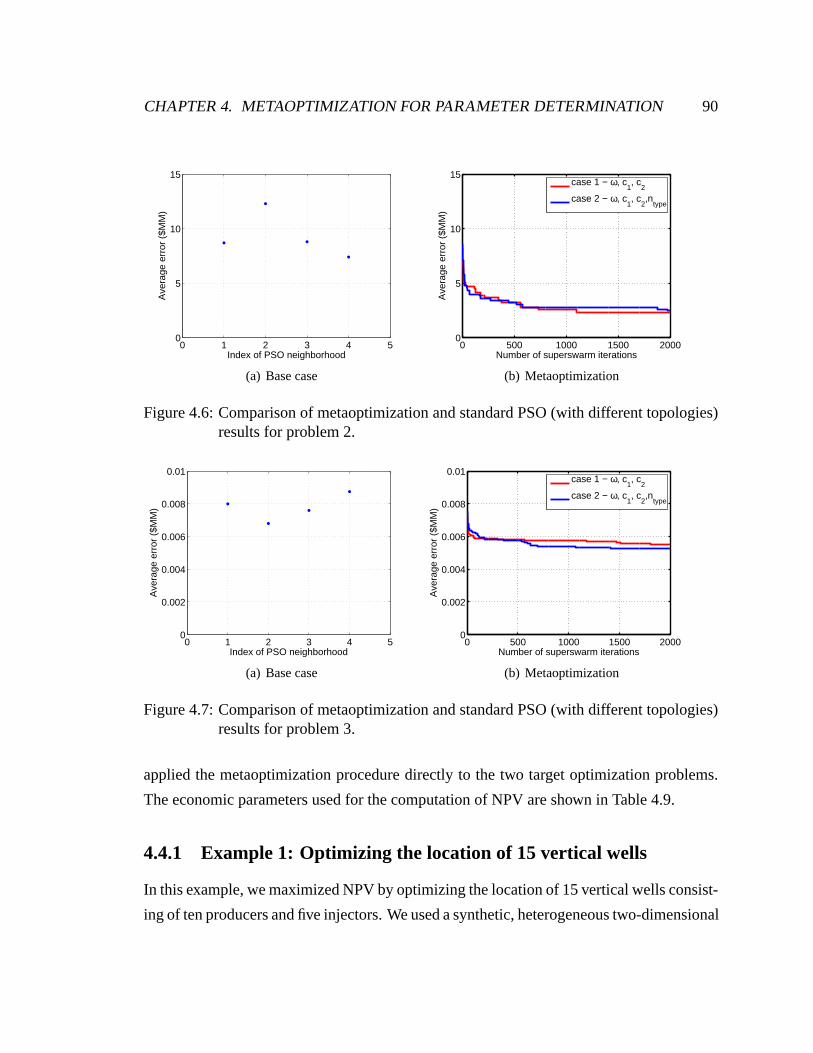
CHAPTER 4. METAOPTIMIZATION FOR PARAMETER DETERMINATION 90
0 1 2 3 4 50
5
10
15
Index of PSO neighborhood
Ave
rage
err
or (
$MM
)
(a) Base case
0 500 1000 1500 20000
5
10
15
Number of superswarm iterations
Ave
rage
err
or (
$MM
)
case 1 − ω, c1, c
2
case 2 − ω, c1, c
2,n
type
(b) Metaoptimization
Figure 4.6: Comparison of metaoptimization and standard PSO(with different topologies)results for problem 2.
0 1 2 3 4 50
0.002
0.004
0.006
0.008
0.01
Index of PSO neighborhood
Ave
rage
err
or (
$MM
)
(a) Base case
0 500 1000 1500 20000
0.002
0.004
0.006
0.008
0.01
Number of superswarm iterations
Ave
rage
err
or (
$MM
)
case 1 − ω, c1, c
2
case 2 − ω, c1, c
2,n
type
(b) Metaoptimization
Figure 4.7: Comparison of metaoptimization and standard PSO(with different topologies)results for problem 3.
applied the metaoptimization procedure directly to the twotarget optimization problems.
The economic parameters used for the computation of NPV are shown in Table 4.9.
4.4.1 Example 1: Optimizing the location of 15 vertical wells
In this example, we maximized NPV by optimizing the locationof 15 vertical wells consist-
ing of ten producers and five injectors. We used a synthetic, heterogeneous two-dimensional
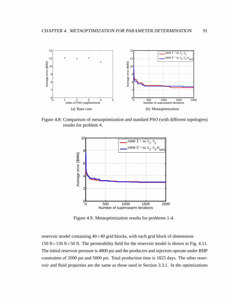
CHAPTER 4. METAOPTIMIZATION FOR PARAMETER DETERMINATION 91
0 1 2 3 4 56
7
8
9
10
11
12
Index of PSO neighborhood
Ave
rage
err
or (
$MM
)
(a) Base case
0 500 1000 1500 20006
7
8
9
10
11
12
Number of superswarm iterations
Ave
rage
err
or (
$MM
)
case 1 − ω, c1, c
2
case 2 − ω, c1, c
2,n
type
(b) Metaoptimization
Figure 4.8: Comparison of metaoptimization and standard PSO(with different topologies)results for problem 4.
0 500 1000 1500 20000
2
4
6
8
10
Number of superswarm iterations
Ave
rage
err
or (
$MM
)
case 1 − ω, c1, c
2
case 2 − ω, c1, c
2,n
type
Figure 4.9: Metaoptimization results for problems 1-4.
reservoir model containing 40×40 grid blocks, with each grid block of dimensions
150 ft×150 ft×50 ft. The permeability field for the reservoir model is shownin Fig. 4.11.
The initial reservoir pressure is 4800 psi and the producersand injectors operate under BHP
constraints of 2000 psi and 5000 psi. Total production time is 1825 days. The other reser-
voir and fluid properties are the same as those used in Section3.3.1. In the optimizations
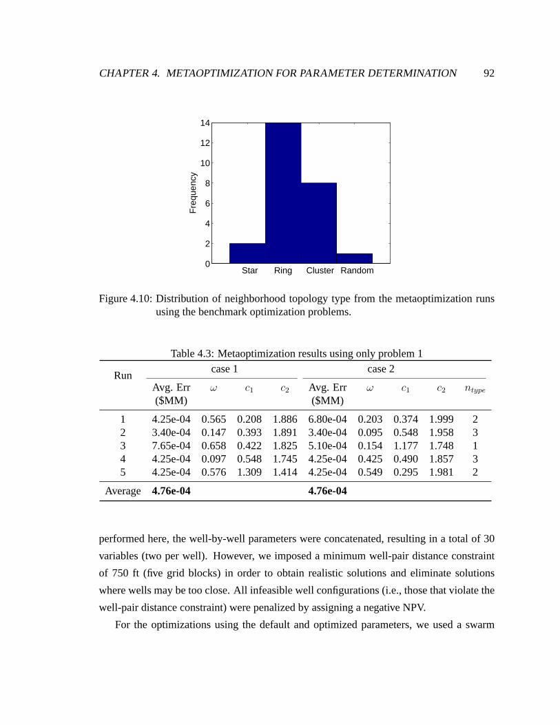
CHAPTER 4. METAOPTIMIZATION FOR PARAMETER DETERMINATION 92
Star Ring Cluster Random0
2
4
6
8
10
12
14
Fre
quen
cy
Figure 4.10: Distribution of neighborhood topology type from the metaoptimization runsusing the benchmark optimization problems.
Table 4.3: Metaoptimization results using only problem 1
Runcase 1 case 2
Avg. Err ω c1 c2 Avg. Err ω c1 c2 ntype
($MM) ($MM)
1 4.25e-04 0.565 0.208 1.886 6.80e-04 0.203 0.374 1.999 22 3.40e-04 0.147 0.393 1.891 3.40e-04 0.095 0.548 1.958 33 7.65e-04 0.658 0.422 1.825 5.10e-04 0.154 1.177 1.748 14 4.25e-04 0.097 0.548 1.745 4.25e-04 0.425 0.490 1.857 35 4.25e-04 0.576 1.309 1.414 4.25e-04 0.549 0.295 1.981 2
Average 4.76e-04 4.76e-04
performed here, the well-by-well parameters were concatenated, resulting in a total of 30
variables (two per well). However, we imposed a minimum well-pair distance constraint
of 750 ft (five grid blocks) in order to obtain realistic solutions and eliminate solutions
where wells may be too close. All infeasible well configurations (i.e., those that violate the
well-pair distance constraint) were penalized by assigning a negative NPV.
For the optimizations using the default and optimized parameters, we used a swarm
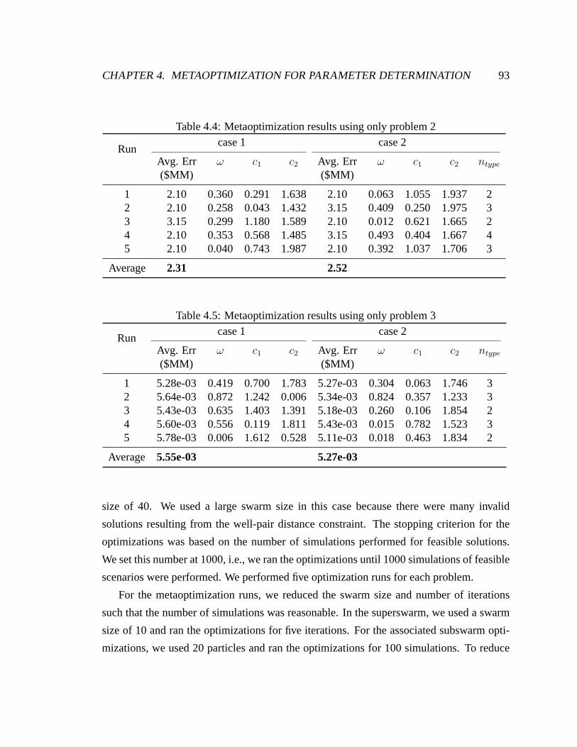
CHAPTER 4. METAOPTIMIZATION FOR PARAMETER DETERMINATION 93
Table 4.4: Metaoptimization results using only problem 2
Runcase 1 case 2
Avg. Err ω c1 c2 Avg. Err ω c1 c2 ntype
($MM) ($MM)
1 2.10 0.360 0.291 1.638 2.10 0.063 1.055 1.937 22 2.10 0.258 0.043 1.432 3.15 0.409 0.250 1.975 33 3.15 0.299 1.180 1.589 2.10 0.012 0.621 1.665 24 2.10 0.353 0.568 1.485 3.15 0.493 0.404 1.667 45 2.10 0.040 0.743 1.987 2.10 0.392 1.037 1.706 3
Average 2.31 2.52
Table 4.5: Metaoptimization results using only problem 3
Runcase 1 case 2
Avg. Err ω c1 c2 Avg. Err ω c1 c2 ntype
($MM) ($MM)
1 5.28e-03 0.419 0.700 1.783 5.27e-03 0.304 0.063 1.746 32 5.64e-03 0.872 1.242 0.006 5.34e-03 0.824 0.357 1.233 33 5.43e-03 0.635 1.403 1.391 5.18e-03 0.260 0.106 1.854 24 5.60e-03 0.556 0.119 1.811 5.43e-03 0.015 0.782 1.523 35 5.78e-03 0.006 1.612 0.528 5.11e-03 0.018 0.463 1.834 2
Average 5.55e-03 5.27e-03
size of 40. We used a large swarm size in this case because there were many invalid
solutions resulting from the well-pair distance constraint. The stopping criterion for the
optimizations was based on the number of simulations performed for feasible solutions.
We set this number at 1000, i.e., we ran the optimizations until 1000 simulations of feasible
scenarios were performed. We performed five optimization runs for each problem.
For the metaoptimization runs, we reduced the swarm size andnumber of iterations
such that the number of simulations was reasonable. In the superswarm, we used a swarm
size of 10 and ran the optimizations for five iterations. For the associated subswarm opti-
mizations, we used 20 particles and ran the optimizations for 100 simulations. To reduce

CHAPTER 4. METAOPTIMIZATION FOR PARAMETER DETERMINATION 94
Table 4.6: Metaoptimization results using only problem 4
Runcase 1 case 2
Avg. Err ω c1 c2 Avg. Err ω c1 c2 ntype
($MM) ($MM)
1 7.35 0.110 1.899 1.827 7.69 0.687 0.005 1.419 22 7.43 0.071 0.141 1.764 7.09 0.323 0.187 1.934 33 7.24 0.094 1.340 1.872 7.20 0.413 1.867 1.762 24 7.03 0.343 0.263 1.368 7.63 0.084 0.241 1.690 15 7.45 0.993 0.032 1.692 7.33 0.220 0.029 1.875 2
Average 7.30 7.34
Table 4.7: Metaoptimization results using all benchmark problems
Runcase 1 case 2
Avg. Err ω c1 c2 Avg. Err ω c1 c2 ntype
($MM) ($MM)
1 2.58 0.493 0.665 1.467 2.86 0.970 1.152 1.950 22 2.86 0.066 0.552 1.781 2.84 0.819 0.178 1.446 23 3.57 0.254 1.438 1.452 3.47 0.986 1.226 1.911 24 3.08 0.676 0.072 1.919 3.06 0.010 0.858 1.487 15 2.70 0.368 1.318 1.562 2.73 0.285 0.639 1.805 2
Average 2.96 2.99
Table 4.8: Default and optimized PSO parameters
Parameter DefaultOptimized Parameters
case 1 case 2
ω 0.721 0.493 0.285c1 1.193 0.665 0.639c2 1.193 1.467 1.805
ntype Random Random Ring
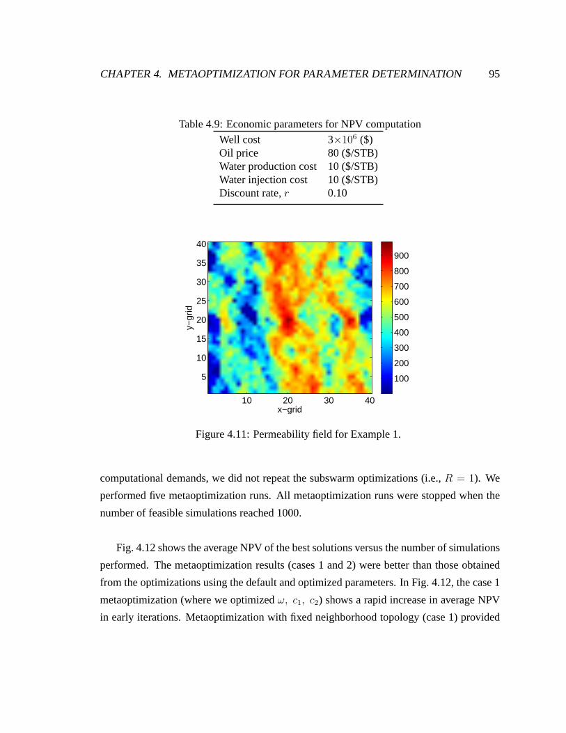
CHAPTER 4. METAOPTIMIZATION FOR PARAMETER DETERMINATION 95
Table 4.9: Economic parameters for NPV computation
Well cost 3×10⁶ ($)Oil price 80 ($/STB)Water production cost 10 ($/STB)Water injection cost 10 ($/STB)Discount rate,r 0.10
x−grid
y−gr
id
10 20 30 40
5
10
15
20
25
30
35
40
100
200
300
400
500
600
700
800
900
Figure 4.11: Permeability field for Example 1.
computational demands, we did not repeat the subswarm optimizations (i.e.,R = 1). We
performed five metaoptimization runs. All metaoptimization runs were stopped when the
number of feasible simulations reached 1000.
Fig. 4.12 shows the average NPV of the best solutions versus the number of simulations
performed. The metaoptimization results (cases 1 and 2) were better than those obtained
from the optimizations using the default and optimized parameters. In Fig. 4.12, the case 1
metaoptimization (where we optimizedω, c1, c2) shows a rapid increase in average NPV
in early iterations. Metaoptimization with fixed neighborhood topology (case 1) provided
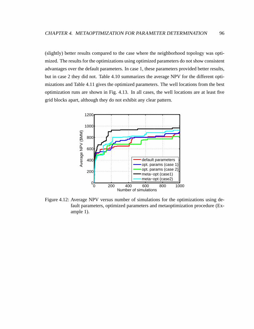
CHAPTER 4. METAOPTIMIZATION FOR PARAMETER DETERMINATION 96
(slightly) better results compared to the case where the neighborhood topology was opti-
mized. The results for the optimizations using optimized parameters do not show consistent
advantages over the default parameters. In case 1, these parameters provided better results,
but in case 2 they did not. Table 4.10 summarizes the average NPV for the different opti-
mizations and Table 4.11 gives the optimized parameters. The well locations from the best
optimization runs are shown in Fig. 4.13. In all cases, the well locations are at least five
grid blocks apart, although they do not exhibit any clear pattern.
0 200 400 600 800 10000
200
400
600
800
1000
1200
Number of simulations
Ave
rage
NP
V (
$MM
)
default parametersopt. params (case 1)opt. params (case 2)meta−opt (case1)meta−opt (case2)
Figure 4.12: Average NPV versus number of simulations for the optimizations using de-fault parameters, optimized parameters and metaoptimization procedure (Ex-ample 1).
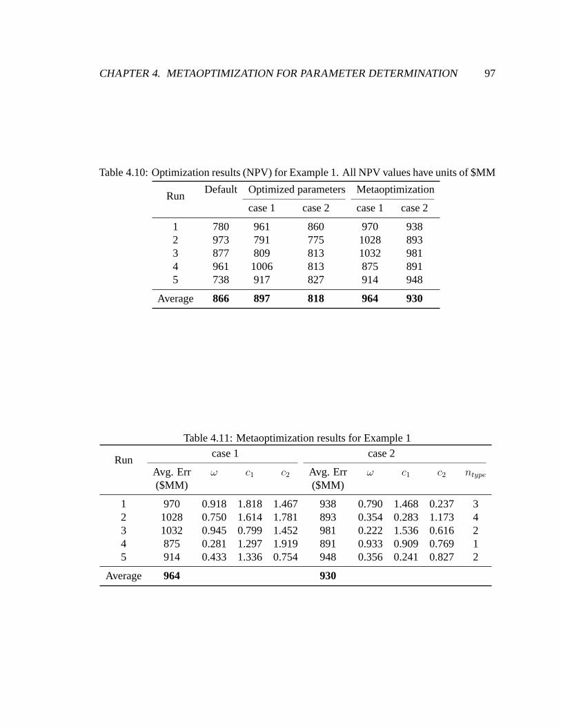
CHAPTER 4. METAOPTIMIZATION FOR PARAMETER DETERMINATION 97
Table 4.10: Optimization results (NPV) for Example 1. All NPV values have units of $MM
RunDefault Optimized parameters Metaoptimization
case 1 case 2 case 1 case 2
1 780 961 860 970 9382 973 791 775 1028 8933 877 809 813 1032 9814 961 1006 813 875 8915 738 917 827 914 948
Average 866 897 818 964 930
Table 4.11: Metaoptimization results for Example 1
Runcase 1 case 2
Avg. Err ω c1 c2 Avg. Err ω c1 c2 ntype
($MM) ($MM)
1 970 0.918 1.818 1.467 938 0.790 1.468 0.237 32 1028 0.750 1.614 1.781 893 0.354 0.283 1.173 43 1032 0.945 0.799 1.452 981 0.222 1.536 0.616 24 875 0.281 1.297 1.919 891 0.933 0.909 0.769 15 914 0.433 1.336 0.754 948 0.356 0.241 0.827 2
Average 964 930
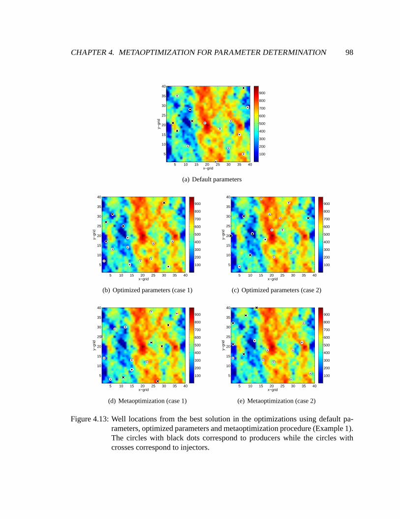
CHAPTER 4. METAOPTIMIZATION FOR PARAMETER DETERMINATION 98
x−grid
y−gr
id
5 10 15 20 25 30 35 40
5
10
15
20
25
30
35
40
100
200
300
400
500
600
700
800
900
(a) Default parameters
x−grid
y−gr
id
5 10 15 20 25 30 35 40
5
10
15
20
25
30
35
40
100
200
300
400
500
600
700
800
900
(b) Optimized parameters (case 1)
x−grid
y−gr
id
5 10 15 20 25 30 35 40
5
10
15
20
25
30
35
40
100
200
300
400
500
600
700
800
900
(c) Optimized parameters (case 2)
x−grid
y−gr
id
5 10 15 20 25 30 35 40
5
10
15
20
25
30
35
40
100
200
300
400
500
600
700
800
900
(d) Metaoptimization (case 1)
x−grid
y−gr
id
5 10 15 20 25 30 35 40
5
10
15
20
25
30
35
40
100
200
300
400
500
600
700
800
900
(e) Metaoptimization (case 2)
Figure 4.13: Well locations from the best solution in the optimizations using default pa-rameters, optimized parameters and metaoptimization procedure (Example 1).The circles with black dots correspond to producers while the circles withcrosses correspond to injectors.
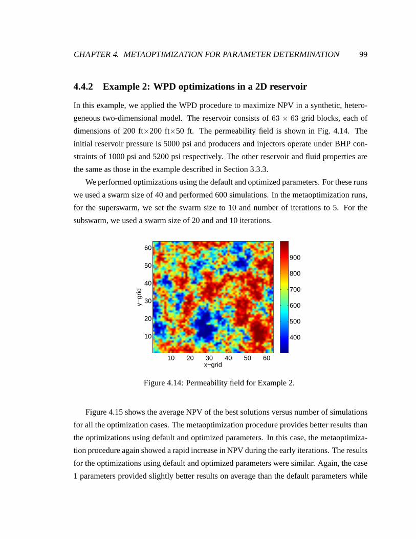
CHAPTER 4. METAOPTIMIZATION FOR PARAMETER DETERMINATION 99
4.4.2 Example 2: WPD optimizations in a 2D reservoir
In this example, we applied the WPD procedure to maximize NPV in a synthetic, hetero-
geneous two-dimensional model. The reservoir consists of63 × 63 grid blocks, each of
dimensions of 200 ft×200 ft×50 ft. The permeability field is shown in Fig. 4.14. The
initial reservoir pressure is 5000 psi and producers and injectors operate under BHP con-
straints of 1000 psi and 5200 psi respectively. The other reservoir and fluid properties are
the same as those in the example described in Section 3.3.3.
We performed optimizations using the default and optimizedparameters. For these runs
we used a swarm size of 40 and performed 600 simulations. In the metaoptimization runs,
for the superswarm, we set the swarm size to 10 and number of iterations to 5. For the
subswarm, we used a swarm size of 20 and and 10 iterations.
x−grid
y−gr
id
10 20 30 40 50 60
10
20
30
40
50
60
400
500
600
700
800
900
Figure 4.14: Permeability field for Example 2.
Figure 4.15 shows the average NPV of the best solutions versus number of simulations
for all the optimization cases. The metaoptimization procedure provides better results than
the optimizations using default and optimized parameters.In this case, the metaoptimiza-
tion procedure again showed a rapid increase in NPV during the early iterations. The results
for the optimizations using default and optimized parameters were similar. Again, the case
1 parameters provided slightly better results on average than the default parameters while
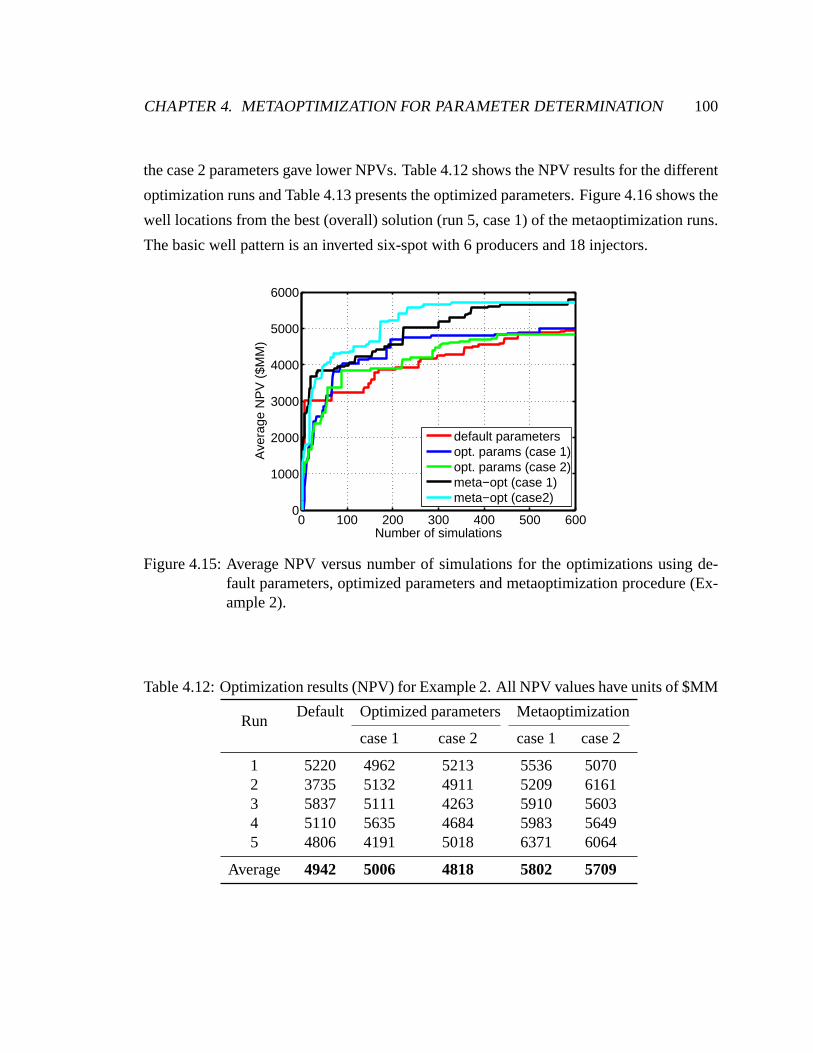
CHAPTER 4. METAOPTIMIZATION FOR PARAMETER DETERMINATION 100
the case 2 parameters gave lower NPVs. Table 4.12 shows the NPV results for the different
optimization runs and Table 4.13 presents the optimized parameters. Figure 4.16 shows the
well locations from the best (overall) solution (run 5, case1) of the metaoptimization runs.
The basic well pattern is an inverted six-spot with 6 producers and 18 injectors.
0 100 200 300 400 500 6000
1000
2000
3000
4000
5000
6000
Number of simulations
Ave
rage
NP
V (
$MM
)
default parametersopt. params (case 1)opt. params (case 2)meta−opt (case 1)meta−opt (case2)
Figure 4.15: Average NPV versus number of simulations for the optimizations using de-fault parameters, optimized parameters and metaoptimization procedure (Ex-ample 2).
Table 4.12: Optimization results (NPV) for Example 2. All NPV values have units of $MM
RunDefault Optimized parameters Metaoptimization
case 1 case 2 case 1 case 2
1 5220 4962 5213 5536 50702 3735 5132 4911 5209 61613 5837 5111 4263 5910 56034 5110 5635 4684 5983 56495 4806 4191 5018 6371 6064
Average 4942 5006 4818 5802 5709
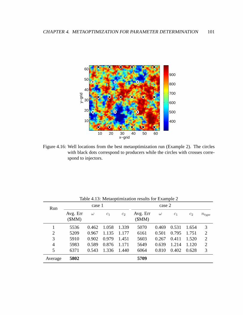
CHAPTER 4. METAOPTIMIZATION FOR PARAMETER DETERMINATION 101
x−grid
y−gr
id
10 20 30 40 50 60
10
20
30
40
50
60
400
500
600
700
800
900
Figure 4.16: Well locations from the best metaoptimizationrun (Example 2). The circleswith black dots correspond to producers while the circles with crosses corre-spond to injectors.
Table 4.13: Metaoptimization results for Example 2
Runcase 1 case 2
Avg. Err ω c1 c2 Avg. Err ω c1 c2 ntype
($MM) ($MM)
1 5536 0.462 1.058 1.339 5070 0.469 0.531 1.654 32 5209 0.967 1.135 1.177 6161 0.501 0.795 1.751 23 5910 0.902 0.979 1.451 5603 0.267 0.411 1.520 24 5983 0.589 0.876 1.171 5649 0.639 1.214 1.120 25 6371 0.543 1.336 1.440 6064 0.810 0.402 0.628 3
Average 5802 5709
CHAPTER 4. METAOPTIMIZATION FOR PARAMETER DETERMINATION 102
4.5 Further Assessment of the Metaoptimization Results
Here, we compared the values of the optimized PSO parameters(ω, c1, andc2) obtained
from the metaoptimization runs to those obtained by sampling ω, c1, andc2 exhaustively
for the Rosenbrock and Griewank mathematical functions. Figure 4.17 shows plots ofφ =
0.5(c1 + c2) versusω for both the Rosenbrock and Griewank functions with the contours
showing the average objective function values over severalruns (the two exhaustive plots
are taken from [66]). In Figure 4.17, combinations ofω, c1 and c2 that result in low
objective function values are preferred. We have superimposed theω, c1 and c2 values
(indicated by the red dots) obtained from all the metaoptimization runs in this chapter. In
both plots, most of the values ofω, c1, andc2 from the metaoptimization are located in the
regions with low objective function values. The lines on theplot indicate different regions
where a PSO particle trajectory may be convergent or divergent. The interested reader is
referred to [3, 49, 50, 66] for more details regarding these regions. In general, the values
of ω, c1 andc2 from the metaoptimization runs agree well with the conditions required for
stable and convergent PSO particle trajectories describedin [3, 66].
4.6 Summary
In this chapter, we discussed the implementation of the metaoptimization procedure to op-
timize PSO parameters during optimization. Metaoptimization involves the use of two PSO
algorithms, with the first one (superswarm PSO) optimizing the PSO parameters used in the
second one (subswarm PSO). The well placement problems weresolved in the subswarm
PSO using the parameters from the associated superswarm particle. The metaoptimization
procedure was applied for well placement optimization using four benchmark problems.
We performed optimizations first using each test problem separately, and then using all
four problems together. The latter procedure enabled us to determine appropriate parame-
ters for a suite of optimization problems.
We applied the optimized parameters (from the metaoptimizations with the benchmark
problems) to realistic and much larger well placement optimizations. Two well placement

CHAPTER 4. METAOPTIMIZATION FOR PARAMETER DETERMINATION 103
ω
φ
Rosenbrock 10 dimensions
−1 −0.5 0 0.5 10
0.5
1
1.5
2
2.5
3
3.5
4
0.3
0.4
0.5
0.6
0.7
0.8
0.9
(a) Rosenbrock
ω
φ
Griewank 10 dimensions
−1 −0.5 0 0.5 10
0.5
1
1.5
2
2.5
3
3.5
4
−1
−0.5
0
0.5
1
1.5
2
(b) Griewank
Figure 4.17: Comparison of the PSO parameters from the metaoptimization runs to thoseobtained by samplingω, c1 and c2 exhaustively for the Rosenbrock andGriewank functions in 10 dimensions. The background plots of φ = 0.5(c1 +c2) versusω were obtained from [66]. The red dots represent the results fromall metaoptimization runs.
CHAPTER 4. METAOPTIMIZATION FOR PARAMETER DETERMINATION 104
problems were considered including the optimization of 15 vertical wells and WPD opti-
mizations in two-dimensional reservoir models. The use of optimized parameters from the
benchmark problems did not result in optimized NPVs that were significantly larger than
those determined using default parameters for the two problems considered.
We also applied the metaoptimization procedure directly tothe two optimization prob-
lems. We compared metaoptimization results to those from optimizations using the default
and optimized parameters for the same number of simulations. For both optimization prob-
lems, the best results were obtained using metaoptimization, i.e., when the parameters were
directly optimized for the target problems. In addition, metaoptimization showed much
faster increases in average NPV in early iterations for the two problems considered. Thus
the results in this chapter suggest that metaoptimization should be considered for practical
well placement optimization problems.
Chapter 5
Summary and Future Work
In this research, we investigated the use of the particle swarm optimization (PSO) algo-
rithm to optimize the type and location of new wells. We addressed the problem of op-
timizing well locations in large-scale field development involving many wells. We also
addressed issues related to the determination of optimum PSO parameters for well place-
ment optimization. The findings in this dissertation are also relevant for other optimization
problems, e.g., production optimization, and optimizing injection and extraction wells for
contaminated groundwater applications.
5.1 Summary and Conclusions
5.1.1 Particle Swarm Optimization
• The particle swarm optimization (PSO) algorithm was implemented and applied
to the optimization of well locations and type. The algorithm is stochastic and
population-based. The individual solutions, called particles, interact with each other
and exchange information regarding the search space. Particles interact with other
particles in their neighborhood. We implemented differentparticle neighborhood
topologies, which can affect algorithm performance.
• The PSO algorithm was applied to several well placement optimization problems of
105
CHAPTER 5. SUMMARY AND FUTURE WORK 106
varying complexity. We considered problems with differentnumbers of wells, differ-
ent types of wells (vertical, deviated, multilateral), anddifferent sizes of the search
space. Multiple geological realizations were used in some cases. We compared the
optimization results to those obtained using a binary GA (bGA). In all examples
considered, we demonstrated that the PSO algorithm provided comparable or better
results on average than the bGA. For a case in which the globaloptimum was known
(through exhaustive sampling), PSO was shown to achieve theglobal minimum with
fewer function evaluations than bGA. For this case, the performance of the PSO and
GA algorithms improved when the swarm/population size and/or the number of iter-
ations were increased. Our findings regarding the performance of PSO are consistent
with those from a related application involving the optimization of extraction well
locations in contaminated groundwater applications [63].
• The PSO algorithm was used also for other applications. It was used as the core
optimization algorithm in the well pattern optimization (WPO) procedure and was
applied for optimizing PSO parameters in the metaoptimization procedure.
5.1.2 Well Pattern Optimization
• A new procedure for optimizing well placement in large-scale field developments
involving many wells was developed. The new algorithm, called well pattern opti-
mization (WPO), consists of a well pattern description (WPD) incorporated into a
core optimization algorithm. In the well pattern descriptions, each solution consists
of a representation of a particular well pattern along with pattern operators that alter
the size, shape, and orientation of the pattern. Many different well patterns can be
considered within WPD. It is the parameters associated with the pattern descriptions
and operators that are determined during the optimizations. The encoded well pat-
terns are repeated across the field, which enables the optimum number of wells to be
determined as part of the solution. A desirable feature of WPDis that the compu-
tational complexity of the optimization is essentially independent of the number of
wells considered.
• A well-by-well perturbation (WWP) procedure was also developed. WWP, which
CHAPTER 5. SUMMARY AND FUTURE WORK 107
can be applied as an optional second phase of the optimization, entails a local pertur-
bation of the well locations obtained from the WPD optimization. For the underlying
(core) optimization algorithm, we used particle swarm optimization (PSO).
• The WPO procedure was applied to four example cases. Several variants of WPO
were considered including the use of one versus four operators for each potential
solution and the use of WWP following optimization using WPD. The overall opti-
mization procedure was shown to result in significant increases in the objective func-
tion, particularly at early iterations, in all cases. In oneexample the WPO results for
net present value (NPV) were compared to those for standard well patterns of various
sizes. The NPVs using WPO were seen to be significantly larger than those for stan-
dard well patterns, highlighting the potential benefit of the algorithm for identifying
promising development scenarios. Significant improvementin NPV was obtained by
performing WWP optimizations on the best solution obtained using WPD. For the
two examples in which WWP was applied, average improvements inNPV of 22%
and 34% over the best WPD solutions were achieved. We also compared WPD re-
sults to those obtained from optimizations using concatenated well parameters and
found the WPO procedure to provide better solutions.
5.1.3 Metaoptimization for Parameter Determination
• A procedure for determining optimum PSO parameters was implemented and tested.
This procedure, called metaoptimization, optimizes PSO parameters during opti-
mization. Metaoptimization requires two PSO algorithms, where the first algorithm
optimizes PSO parameters, and the second algorithm optimizes a given optimization
problem or problems using the PSO parameters from the first algorithm.
• We applied the metaoptimization procedure to determine optimum PSO parame-
ters using four benchmark well placement optimization problems. In the metaop-
timizations, we considered two cases. In case 1, we optimized PSO parameters
ω, c1, c2, while in case 2, we optimized the neighborhood topology type in addition
to ω, c1, c2. We showed that metaoptimization provided results better than those
CHAPTER 5. SUMMARY AND FUTURE WORK 108
for PSO with unoptimized parameters. Next, we applied the metaoptimization to all
four benchmark problems in order to determine PSO parameters that are optimal for
multiple problems.
• We applied the optimized PSO parameters and metaoptimization to two optimization
problems including optimizing the location of 15 vertical wells (consisting of ten pro-
ducers and five injectors) and WPD optimizations in heterogeneous two-dimensional
reservoirs. For these examples, metaoptimization was shown to provide the best re-
sults.
5.2 Recommendations for Future Work
• In the PSO optimizations in Chapter 2, we represent solutionsusing well-by-well
concatenation. For these optimizations, the PSO algorithmdid not include any con-
straint handling. If well-by-well parameter concatenation is to be used, it will be
necessary to incorporate constraint handling methods in order to obtain practically
acceptable well configurations. This can be achieved by several methods. One ap-
proach is to use penalty function methods and penalize all infeasible solutions. We
used this method for an example problem in Chapter 4. Other approaches include
feasibility preserving and repair methods [3]. In feasibility preserving methods, the
particle positions are computed so that constraints are notviolated. In repair methods,
special operators are used to repair an infeasible particleor to adjust it so it satisfies
all constraints. A similar technique was implemented for GAin [29] to handle gen-
eral well placement optimization constraints. Other constraint handling techniques
for PSO are described in [3].
• Potentially the performance of the PSO algorithm could be improved further by in-
corporating methods to increase or preserve the diversity of the particles. As the PSO
particles converge, they may exhibit a tendency to cluster around the best solution,
especially when the star neighborhood topology is used. Procedures for improving
the diversity of particles should be explored. For example,if the objective function
does not improve over a prescribed number of iterations, a fraction of the particles
CHAPTER 5. SUMMARY AND FUTURE WORK 109
could be reinitialized around their local best positions [3].
• The PSO performance could also be improved by balancing exploration and exploita-
tion within the optimization. One way to achieve this is to use a generalized PSO
where∆t (in the velocity and position update equations) can take values other than
unity [50, 49].
• It may be of interest to investigate specialized PSO particle neighborhood topolo-
gies. Also, other variants of the two-phase optimization strategy (WPD followed by
WWP) should be considered. In addition, the number of patternsconsidered could
be increased to include other well patterns, e.g., the 13-spot well pattern. Such addi-
tions do not lead to an increase in the number of variables required to represent the
patterns in WPD.
• The WPO procedure should be applied to larger models (in arealextent) than those
considered here. It will also be of interest to test the WPO procedure for practical
problems. For such cases, it may be useful to extend the WWP procedure to optimize
completion interval, to allow for the elimination of particular wells, etc.
• The efficiency of the PSO and WPO algorithms may be improved through the use
of surrogate (proxy) simulation models, e.g., kriging, statistical proxies, and neural
networks. This would act to reduce the number of time consuming simulations re-
quired. Use of a hybrid optimization approach involving thecombination of PSO
with a local optimizer may also prove effective.
• The metaoptimization procedure was demonstrated to be effective at optimizing PSO
parameters and providing better solutions, on average, relative to those achieved us-
ing untuned/unoptimized PSO parameters. However, the procedure is computation-
ally intensive because of the many function evaluations required. Surrogate models
should be incorporated into the metaoptimization procedure to reduce the computa-
tional demands and to enable this approach to be used for practical applications.
• The combined optimization of well placement and well control should be considered.
This will be very demanding computationally, so efficient optimization strategies will

CHAPTER 5. SUMMARY AND FUTURE WORK 110
need to be devised.
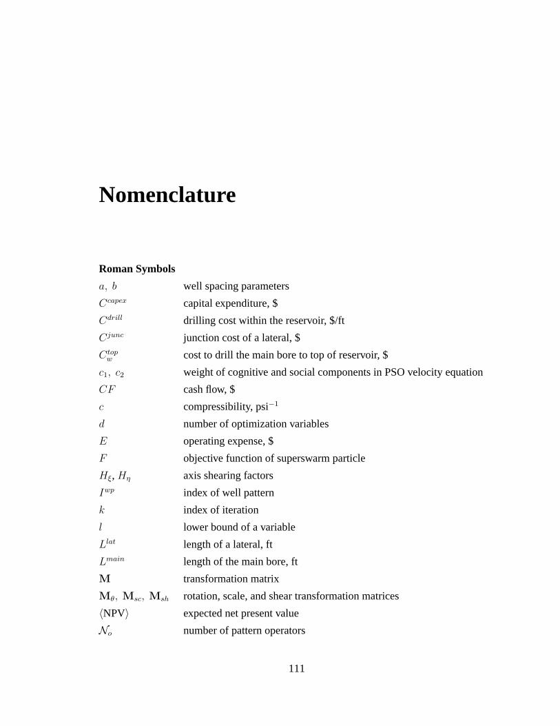
Nomenclature
Roman Symbols
a, b well spacing parameters
Ccapex capital expenditure, $
Cdrill drilling cost within the reservoir, $/ft
Cjunc junction cost of a lateral, $
Ctopw cost to drill the main bore to top of reservoir, $
c1, c2 weight of cognitive and social components in PSO velocity equation
CF cash flow, $
c compressibility, psi−1
d number of optimization variables
E operating expense, $
F objective function of superswarm particle
Hξ, Hη axis shearing factors
Iwp index of well pattern
k index of iteration
l lower bound of a variable
Llat length of a lateral, ft
Lmain length of the main bore, ft
M transformation matrix
Mθ, Msc, Msh rotation, scale, and shear transformation matrices
〈NPV〉 expected net present value
No number of pattern operators
111
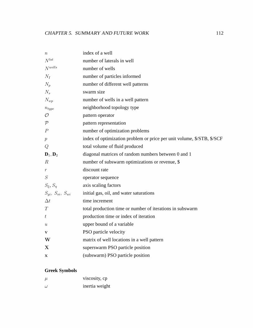
CHAPTER 5. SUMMARY AND FUTURE WORK 112
n index of a well
N lat number of laterals in well
Nwells number of wells
NI number of particles informed
Np number of different well patterns
Ns swarm size
Nwp number of wells in a well pattern
ntype neighborhood topology type
O pattern operator
P pattern representation
P number of optimization problems
p index of optimization problem or price per unit volume, $/STB, $/SCF
Q total volume of fluid produced
D1, D2 diagonal matrices of random numbers between 0 and 1
R number of subswarm optimizations or revenue, $
r discount rate
S operator sequence
Sξ, Sη axis scaling factors
Sgi, Soi, Swi initial gas, oil, and water saturations
∆t time increment
T total production time or number of iterations in subswarm
t production time or index of iteration
u upper bound of a variable
v PSO particle velocity
W matrix of well locations in a well pattern
X superswarm PSO particle position
x (subswarm) PSO particle position
Greek Symbols
µ viscosity, cp
ω inertia weight
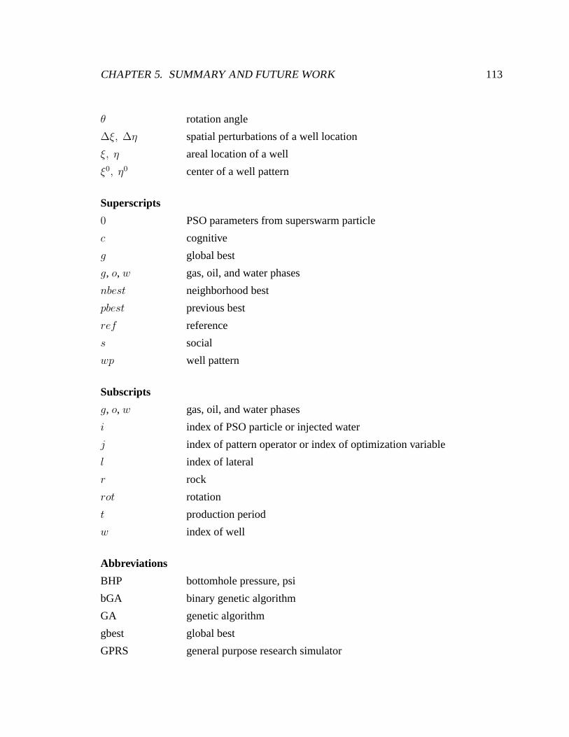
CHAPTER 5. SUMMARY AND FUTURE WORK 113
θ rotation angle
∆ξ, ∆η spatial perturbations of a well location
ξ, η areal location of a well
ξ0, η0 center of a well pattern
Superscripts
0 PSO parameters from superswarm particle
c cognitive
g global best
g, o, w gas, oil, and water phases
nbest neighborhood best
pbest previous best
ref reference
s social
wp well pattern
Subscripts
g, o, w gas, oil, and water phases
i index of PSO particle or injected water
j index of pattern operator or index of optimization variable
l index of lateral
r rock
rot rotation
t production period
w index of well
Abbreviations
BHP bottomhole pressure, psi
bGA binary genetic algorithm
GA genetic algorithm
gbest global best
GPRS general purpose research simulator

CHAPTER 5. SUMMARY AND FUTURE WORK 114
lbest local best
MM, $MM million, million dollars
NPV net present value
PSO particle swarm optimization
SimA simulated annealing
SPSA simultaneous perturbation stochastic approximation
WPD well pattern description
WPO well pattern optimization
WWP well-by-well perturbation
References
[1] Y. Collette and P. Siarry.Multiobjective Optimization: Principles and Case Studies.
Springer-Verlag, Berlin, Germany, 2003.
[2] M. Clerc. Particle Swarm Optimization. iSTE, London, England, 2006.
[3] A. P. Engelbrecht.Fundamentals of Computational Swarm Intelligence. Wiley, West
Sussex, England, 2005.
[4] S. Kirkpatrick, C. D. Gelatt, Jr., and M. P. Vecchi. Optimization by simulated anneal-
ing. Science, 220:671–680, 1983.
[5] B. L. Beckner and X. Song. Field development planning usingsimulated annealing
- optimal economic well scheduling and placement. Paper SPE30650 presented at
the SPE Annual Technical Conference and Exhibition, Dallas,Texas, U.S.A., 22-25
October, 1995.
[6] Z. Michalewicz and D. B. Fogel.How to Solve It: Modern Heuristics. Springer-
Verlag, Berlin, Germany, 2004.
[7] R. L. Haupt and S. E. Haupt.Practical Genetic Algorithms. John Wiley & Sons, Inc.,
New Jersey, U.S.A., 2004.
[8] W. Bangerth, H. Klie, M. F. Wheeler, P. L. Stoffa, and M. K. Sen. On optimization
algorithms for the reservoir oil well placement problem.Computational Geosciences,
10:303–319, 2006.
115
REFERENCES 116
[9] K. P. Norrena and C. V. Deutsch. Automatic determination of well placement sub-
ject to geostatistical and economic constraints. Paper SPE78996 presented at the
SPE International Thermal Operations and Heavy Oil Symposium and International
Horizontal Well Technology Conference, Calgary, Alberta, Canada, 4-7 November,
2002.
[10] K. L. Franstrom and M. L. Litvak. Automatic simulation algorithm for appraisal of
future infill development potential of Prudhoe Bay. Paper SPE59374 presented at the
SPE/DOE Improved Oil Recovery Symposium, Tulsa, Oklahoma, U.S.A., 3-5 April,
2000.
[11] M. Litvak, B. Gane, G. Williams, M. Mansfield, P. Angert, C.Macdonald, L. McMur-
ray, R. Skinner, and G.J. Walker. Field development optimization technology. Paper
SPE 106426 presented at the SPE Reservoir Simulation Symposium, Houston, Texas,
U.S.A., 26-28 February, 2007.
[12] G. J. J. Williams, M. Mansfield, D. G. Macdonald, and M. D.Bush. Top-down reser-
voir modeling. Paper SPE 89974 presented at the SPE Annual Technical Conference
and Exhibition, Houston, Texas, U.S.A., 26-29 September, 2004.
[13] V. Artus, L. J. Durlofsky, J. E. Onwunalu, and K. Aziz. Optimization of nonconven-
tional wells under uncertainty using statistical proxies.Computational Geosciences,
10(4):389–404, 2006.
[14] A. C. Bittencourt and R. N. Horne. Reservoir development anddesign optimization.
Paper SPE 38895 presented at the SPE Annual Technical Conference and Exhibition,
San Antonio, Texas, U.S.A., 5-8 October, 1997.
[15] M. Morravvej Farshi. Master’s thesis. Improving genetic algorithms for optimum
well placement, M.S. thesis, Department of Energy ResourcesEngineering, Stanford
University, 2008.
REFERENCES 117
[16] B. Guyaguler and R. N. Horne. Uncertainty assessment of well placement optimiza-
tion. Paper SPE 71625 presented at the SPE Annual Technical Conference and Exhi-
bition, New Orleans, Louisiana, U.S.A., 30 September - 3 October, 2001.
[17] B. Guyaguler, R. N. Horne, L. Rogers, and J. J. Rosenzweig. Optimization of well
placement in a Gulf of Mexico waterflooding project.Reservoir Evaluation and En-
gineering, 5(3):229–236, 2002.
[18] J. E. Onwunalu. Master’s thesis. Optimization of nonconventional well placement
using genetic algorithms and statistical proxy, M.S. thesis, Department of Energy
Resources Engineering, Stanford University, 2006.
[19] Y. J. Tupac, L. Faletti, M. A. C. Pacheco, and M. M. B. R. Vellasco. Evolutionary
optimization of oil field development. Paper SPE 107552 presented at the SPE Digital
Energy Conference and Exhibition, Houston, Texas, U.S.A., 11-12 April, 2007.
[20] B. Yeten, L. J. Durlofsky, and K. Aziz. Optimization of nonconventional well type,
location and trajectory.SPE Journal, 8(3):200–210, 2003.
[21] U. Ozdogan and R. N. Horne. Optimization of well placement under time-dependent
uncertainty.Reservoir Evaluation and Engineering, 9(2):135–145, 2006.
[22] D. E. Goldberg.Genetic Algorithms in Search, Optimization, and Machine Learning.
Addison-Wesley, Reading, Massachusetts, U.S.A., 1989.
[23] Z. Michalewicz. Genetic Algorithms + Data Structures = Evolution Programs.
Springer-Verlag, Berlin, Germany, 1996.
[24] S. N. Sivananadam and S. N. Deepa.Introduction to Genetic Algorithms. Springer-
Verlag, Berlin, Germany, 2008.
[25] A. Y. Abukhamsin. Optimization of well design and location in a real field, M.S.
thesis, Department of Energy Resources Engineering, Stanford University, 2009.
[26] O. Badru and C. S. Kabir. Well placement optimization in field development. Pa-
per SPE 84191 presented at the SPE Annual Technical Conference and Exhibition,
REFERENCES 118
Denver, Colorado, U.S.A., 5-6 October, 2003.
[27] G. Montes, P. Bartolome, and A. L. Udias. The use of genetic algorithms in well
placement optimization. Paper SPE 69439 presented at the SPE Latin American and
Carribean Petroleum Engineering Conference held in Buenos Aires, Argentina, 25-28
March, 2001.
[28] B. Yeten.Optimum deployment of nonconventional wells. PhD thesis, Stanford Uni-
versity, 2003.
[29] A. A. Emerick, E. Silva, B. Messer, L. F. Almeida, D. Szwarcman, M. A. C. Pacheco,
and M. M. B. R. Vellasco. Well placement optimization using a genetic algorithm
with nonlinear constraints. Paper SPE 118808 presented at the Reservoir Simulation
Symposium, The Woodlands, Texas, U.S.A., 2-4 February, 2009.
[30] D. Y. Ding. Optimization of well placement using evolutionary algorithms. Paper
SPE 113525 presented at the SPE Europec/EAGE Annual Conference and Exhibition,
Rome, Italy, 9-12 June, 2008.
[31] A. Larionov, A. Nifantov, V. Itkin, and V. Alexandrov. Methodology of optimal well
pattern, location and paths in productive formations during oil and gas field develop-
ment planning. Paper SPE 104326 presented at the SPE Russian Oil and Gas Techni-
cal Conference and Exhibition, Moscow, Russia, 3-6 October, 2006.
[32] U. Ozdogan, A. Sahni, B. Yeten, B. Guyaguler, and W. H. Chen.Efficient assessment
and optimization of a deepwater asset development using fixed pattern approach. Pa-
per SPE 95792 presented at the SPE Annual Technical Conference and Exhibition,
Dallas, Texas, U.S.A., 9-12 October, 2005.
[33] J. C. Spall. An overview of the simultaneous perturbation method for efficient opti-
mization. Johns Hopkins Applied Physics Laboratory Technical Digest, 19(4):482–
492, 1998.
[34] R. D. Hazlett and D. K. Babu. Optimal well placement in heterogeneous reservoirs
through semianalytic modeling.SPE Journal, 10(3):286–296, 2005.
REFERENCES 119
[35] C. Wang, G. Li, and A. C. Reynolds. Optimal well placement for production opti-
mization. Paper SPE 111154 presented at the 2007 SPE EasternRegional Meeting,
Lexington, Kentucky, U.S.A., 11-14 October, 2007.
[36] M. J. Zandvliet, M. Handels, G. M. van Essen, D. R. Brouwer,and J. D. Jansen.
Adjoint-based well-placement optimization under production constraints.SPE Jour-
nal, 13(4):392–399, 2008.
[37] P. Sarma and W. H. Chen. Efficient well placement optimization with gradient-based
algorithms and adjoint models. Paper SPE 112257 presented at the SPE Intelligent
Energy Conference and Exhibition, Amsterdam, The Netherlands, 25-27 February,
2008.
[38] S. Vlemmix, G. J. P. Joosten, D. R. Brouwer, and J. D. Jansen. Adjoint-based well
trajectory optimization in a thin oil rim. Paper SPE 121891 presented at the SPE
EUROPEC/EAGE Annual Conference and Exhibition, Amsterdam, The Netherlands,
8-11 June, 2009.
[39] Y. Pan and R. N. Horne. Improved methods for multivariateoptimization of field de-
velopment scheduling and well placement design. Paper SPE 49055 presented at the
SPE Annual Technical Conference and Exhibition, New Orleans, Louisiana, U.S.A.,
27-30 September, 1998.
[40] A. Centilmen, T. Ertekin, and A. S. Grader. Applicationsof neural networks in mul-
tiwell field development. Paper SPE 56433 presented at the SPE Annual Technical
Conference and Exhibition, Houston, Texas, U.S.A., 3-6 October, 1999.
[41] J. E. Onwunalu, M. L. Litvak, L. J. Durlofsky, and K. Aziz. Application of statistical
proxies to speed up field development optimization procedures. Paper SPE 117323
presented at the Abu Dhabi International Petroleum Exhibition and Conference, Abu
Dhabi, U.A.E., 3-6 November, 2008.
[42] F. Zarei, A. Daliri, and N. Alizadeh. The use of neuro-fuzzy proxy in well placement
optimization. Paper SPE 112214 presented at the SPE Intelligent Energy Conference
REFERENCES 120
and Exhibition, Amsterdam, The Netherlands, 25-27 February, 2008.
[43] N. Liu and Y. Jalali. Closing the loop between reservoir modeling and well placement
and positioning. Paper SPE 98198 presented at the SPE Intelligent Energy Conference
and Exhibition, Amsterdam, The Netherlands, 11-13 April, 2006.
[44] R. Volz, K. Burn, M. Litvak, S. Thakur, and S. Skvortsov. Field development optimi-
sation of Siberian giant oil field under uncertainties. Paper SPE 116831 presented at
the SPE Russian Oil and Gas Technical Conference and Exhibition, Moscow, Russia,
28-30 October, 2008.
[45] M. L. Litvak and P. F. Angert. Field development optimization applied to giant oil
fields. Paper SPE 118840 presented at the SPE Reservoir Simulation Symposium,
The Woodlands, Texas, U.S.A., 2-4 February, 2009.
[46] M. L. Litvak, M. L. Gane, and L. McMurray. Field development optimization in
a giant oil field in Azerbaijan and a mature oil field in the North Sea. Paper OTC
18526 presented at the Offshore Technology Conference, Houston, Texas, U.S.A., 30
April-3 May, 2007.
[47] J. Kennedy and R. C. Eberhardt. Particle swarm optimization. InProceedings of the
IEEE International Joint Conference on Neural Networks, pages 1942-1947, IEEE,
December, 1995.
[48] R. C. Eberhardt and J. Kennedy. A new optimizer using particle swarm theory. InPro-
ceedings of the Sixth International Symposium on Micromachine and Human Science,
pages 39–43, 1995.
[49] J. L. F. Martinez and E. G. Gonzalo. The generalized PSO:a new door to PSO
evolution.Artificial Evolution and Applications, 2008:1–15, 2008.
[50] J. L. F. Martinez and E. G. Gonzalo. The PSO family: deduction, stochastic analysis
and comparison.Swarm Intelligence, 3(4):245–273, 2009.
[51] D. E. Goldberg and K. Deb. A comparative analysis of selection schemes used in
REFERENCES 121
genetic algorithms. InFoundations of Genetic Algorithms, pages 69–93. Morgan
Kaufmann, 1991.
[52] R. L. Haupt. Optimum population size and mutation rate for a simple real genetic
algorithm that optimizes array factors. InAntennas and Propagation Society Interna-
tional Symposium, volume 2, pages 1034–1037. IEEE, 2000.
[53] R. Poli, J. Kennedy, and T. Blackwell. Particle swarm optimization. Swarm Intelli-
gence, 1(1):33–57, 2007.
[54] J. Kennedy and R. Mendes. Neighborhood topologies in fully-informed and best-of-
neighborhood particle swarms. InProceedings of the IEEE International Workshop
on Soft Computing in Industrial Applications, pages 45–50. IEEE Press, June 2003.
[55] V. Miranda, H. Keko, and A. J. Duque. Stochastic star communication topology
in evolutionary particle swarms (EPSO).International Journal of Computational
Intelligence Research, 4(2):105–116, 2008.
[56] D. Braendler and T. Hendtlass. The suitability of particle swarm optimisation for
training neural hardware. InInternational Conference on Industrial and Engineering
Applications of Artificial Intelligence and Expert Systems, IEA/AIE, pages 190–199.
Springer, 2002.
[57] R. Chakrabarti, P. K. Chattopadhyay, M. Basu, and C. K. Pangrahi. Particle swarm
optimization technique for dynamic economic dispatch.IE(I) Journal-EL, 87:48–54,
2006.
[58] B. Brandstatter and U. Baumgartner. Particle swarm optimization–mass-spring sys-
tem analogon.IEEE Transactions on Magnetics, 38(2):997–1000, 2002.
[59] D. N. Kumar and M. J. Reddy. Multipurpose reservoir operations using particle swarm
optimization.Water Resources Planning and Management, 133(3):192–201, 2007.
[60] A. R. M. Rao and G. Anandakumar. Optimal placement of sensors for structural sys-
tem identification and health monitoring using a hybrid swarm intelligence technique.
REFERENCES 122
Smart Materials and Structures, 16:2658–2672, 2007.
[61] J. L. F. Martinez and E. G. Gonzalo. Design of a simple andpowerful particle swarm
optimizer. Proceedings of the International Conference on Computational and Math-
ematical Methods in Science and Engineering, CMMSE2009, Gijon, Span, 30 June-3
July, 2009.
[62] O. Uysal and S. Bulkan. Comparison of genetic algorithm and particle swarm opti-
mization for bicriteria permutation flowshop scheduling problem.International Jour-
nal of Computational Intelligence Research, 4(2):159–175, 2008.
[63] L. S. Matott, A. J. Rabideau, and J. R. Craig. Pump-and-treat optimization using
analytic element method flow models.Advances in Water Resources, 29:760–775,
2006.
[64] M. B. Abdelhalim and S. E. D. Habib. Particle swarm optimization for HW/SW
partitioning. In Particle Swarm Optimization, edited by A.Lazinica, pages 49-76,
2009.
[65] Y. Shi and R. C. Eberhardt. A modified particle swarm optimizer. InProceedings of
the IEEE International Conference on Evolutionary Computation, pages 69-73, IEEE
Press, May, 1998.
[66] J. L. F. Martinez, E. G. Gonzalo, and J. P. F. Alvarez. Theoretical analysis of particle
swarm trajectories through a mechanical analogy.International Journal of Computer
Intelligence Research, 2(2-4):93–104, 2006.
[67] M. Clerc and J. Kennedy. The particle swarm – explosion, stability, and convergence
in a multidimensional complex space.IEEE Transactions on Evolutionary Computa-
tions, 6(1):58–73, 2002.
[68] M. Clerc. Stagnation analysis in particle swarm optimization or what happens when
nothing happens. 2006. Technical Report CSM-460, Departmentof Computer Sci-
ence, University of Essex. Edited by Riccardo Poli.
REFERENCES 123
[69] M. Meissner, M. Schmuker, and G. Schneider. Optimized particle swarm optimization
(OPSO) and its application to artificial neural network training. BMC Bioinformatics,
7(125):1–11, 2006.
[70] H. Zhang and M. Ishikawa. Evolutionary canonical particle swarm optimizer - a
proposal of meta-optimization in model selection. In V. Kurkova, R. Neruda, and
J. Koutnik, editors,Artificial Neural Networks - ICANN 2008, Part I, LNCS 5163,
volume 5163/2008, pages 472–481. Springer-Verlag, 2008.
[71] H. Zhang and M. Ishikawa. Evolutionary particle swarm optimization: a metaopti-
mization method with GA for estimating optimal PSO models. In O. Castillo, L. Xu,
and S. Ao, editors,Trends in Intelligent Systems and Computer Engineering, vol-
ume 6, pages 75–90. Springer US, 2008.
[72] J. E. Onwunalu and L. J. Durlofsky. Application of a particle swarm optimization
algorithm for determining optimum well location and type.Computational Geo-
sciences, 14(1):183–198, 2010.
[73] J. E. Onwunalu and L. J. Durlofsky. Development and application of a new well
pattern optimization algorithm for optimizing large-scale field development. 2009.
Paper SPE 124364 presented at the SPE Annual Technical Conference and Exhibition,
New Orleans, Louisiana, USA 4-7 October.
[74] S. Helwig and R. Wanka. Theoretical analysis of initial particle swarm behavior. In
Proceedings of the 10th International Conference on Parallel Problem Solving from
Nature (PPSN08), pages 889–898. Dortmund, Germany, Springer, 13-17 September,
2008.
[75] W. J. Zhang, X. F. Xie, and D. C. Bi. Handling boundary constraints for numerical
optimization by particle swarm flying in periodic search space. InIEEE Congress on
Evolutionary Computation, volume 2, pages 2307–2311,. IEEE, 2004.
[76] A. Carlisle and G. Dozier. An off-the-shelf PSO. InProceedings of Workshop on
Particle Swarm Optimization. Indianapolis, IN, U.S.A., 6-7 April, 2001.
REFERENCES 124
[77] H. Cao. Development of techniques for general purpose research simulator. PhD
thesis, Stanford University, 2002.
[78] Y. Jiang. Techniques for modeling complex reservoirs and advanced wells. PhD
thesis, Stanford University, 2007.
[79] Schlumberger Eclipse. Schedule User Guide 2004A, Chapter 6: Technical descrip-
tion, 2004.
[80] J. T. Alander. On optimal population size of genetic algorithms. InProceedings of
CompEuro ’92 Computer Systems and Software Engineering, pages 65–70, 1992.
[81] K. Deb. Multi-objective optimization using evolutionary algorithms. Wiley, West
Sussex, England, 2001.
[82] F. R. Craig.The Reservoir Engineering Aspects of Waterflooding. SPE Monograph,
Volume 3, 1971.
[83] 3DSL. v2.30 User Manual. Streamsim Technologies Inc.,San Francisco, California,
U.S.A., 2006.